Abstract

We use gauge/gravity duality to investigate the effect of thermal fluctuations on the dissociation of the quarkonium mesons in strongly coupled $(3+1)$-dimensional gauge theories. The purpose of this paper is to introduce a new approach to study the instability and probable first order phase transition of a probe D7-brane in the dual gravity theory. We explicitly show that for the Minkowski embeddings with their tips close to the horizon in the background, the long wavelength thermal fluctuations lead to an imaginary term in their action signaling an instability in the system. Due to this instability, a phase transition is expected. On the gauge theory side, it indicates that the quarkonium mesons are not stable and dissociate in the plasma. Identifying the imaginary part of the probe barne action with the thermal width of the mesons, we observe that the thermal width increases as one decreases the mass of the quarks. Also keeping the mass fixed, thermal width increases by temperature as expected. We will also investigate the effect of the magnetic field on the mass and the thermal width.

1 Introduction and Results

One of the main phenomena observed in Quark-Gluon Plasma (QGP), which is experimentally produced at Relativistic Heavy Ion Collider (RHIC) by colliding two heavy nuclei (such as gold or lead) [1, 2], is quarkonium meson dissociation (or melting) [3]. Quarkonia survive as bound states in the QGP up to a dissociation temperature $T_{diss}$. If the produced QGP is hot enough, $T>T_{diss}$, quarkonia will dissociate in the plasma. In fact the dissociation temperature is realized as a temperature in which meson completely ceases to exist. Since the QGP is a strongly coupled plasma, computing the dissociation temperature perturbatively is not trustworthy and therefore a non-perturbative framework such as gauge/gravity duality will be useful to describe various aspects of the QGP including the dissociation temperature. Of course it is worth mentioning that in thermal QCD in the perturbative high temperature sector, the thermal width of the quarkonium bound state has been analyzed in great detail for instance in [4].

Gauge/gravity duality is a duality between a strongly coupled non-abelian gauge theory and a weakly coupled theory of gravity in a higher dimensional spacetime where the gauge theory lives on the boundary of the spacetime [5, 2]. In fact it is a really helpful duality since by using the gravity dual the analytic calculation for the strongly coupled gauge theory, which is not tractable already, can be done. In particular, the strongly coupled ${\cal{N}}=4$ super Yang-Mills (SYM) theory with gauge group $SU(N)$ in (3+1) dimensions is dual to type IIb supergravity on $AdS_{5}\times S^{5}$. This duality has found many generalizations and specifically it has been successful in describing gauge theories at finite temperature [6]. In short a thermal SYM theory corresponds to the supergravity in an AdS-Schwarzschild black hole background where the temperature of the gauge theory is identified with the Hawking temperature of the black hole.

In the context of gauge/gravity duality, adding fundamental matter (quark) to the strongly coupled SYM theory which lives on the boundary of AdS space is done by introducing the branes into the dual gravity theory that lives in the bulk. This has been proposed in [7] where $N_{f}$ D7-branes are added to the $AdS_{5}\times S^{5}$ background in the probe limit that means $\frac{N_{f}}{N}\ll 1$. This will introduce a matter hypermultiplet in the fundamental representation of the gauge group $SU(N)$ to the SYM theory. The hypermultiplet describes the dynamical quarks living in 3+1 dimensions and the fluctuations of the probe brane explain the meson spectrum of the field theory [2, 8].

The embeddings of the probe brane in the AdS-Schwarzschild black hole background are classified into three types [9]. The Minkowski embeddings (MEs) are those in which the probe brane closes off smoothly above the horizon of the background black hole or equivalently the induced metric on the probe brane has no horizon. For sufficiently large $m_{q}/T$, where $m_{q}$ and $T$ are the bare mass of the quark and temperature of the SYM theory respectively, these embeddings are energetically favorable. In the black hole embedding (BE) case, the induced metric on the brane has an event horizon inherited from the horizon of the black hole living in the background. Between these two types of embeddings, there is a critical embedding for which the tip of the brane touches the horizon at a point.

A (discontinuous) first order phase transition between ME and BE is well known and has been studied in the literature. It is assumed that the mentioned phase transition happens because $c$, which is the expectation value of the dual operator to the mass, is a multi-valued function of $m_{q}$ [9, 10]. However, we present an explicit calculation for this phase transition from ME to BE which is based on considering the effect of thermal fluctuations on the shape of the brane to make its action imaginary. It will be interestingly seen that applying thermal fluctuations’ method previous results of phase transition are reproduced. Moreover this method has the following advantages: 1) This setup is simple and tractable. 2) The results are general and can be applied to various backgrounds or equivalently it provides us with the possibility of describing different strongly coupled SYM theories. 3) Utilizing this setup, we can discuss how thermal fluctuations affect the system. 4) The thermal width for the mesons can be easily defined which is consistent with our physical intuition.

This branes’ shape transition corresponds to the dissociation of the heavy quarkonium mesons on the gauge theory side [2, 9, 10]. The MEs are more favorable in the low temperature limit, i.e. $m_{q}/T\gg 1$ or equivalently $T<T_{diss}$. On the MEs the quarkonium mesons are bounded and their spectrum is discrete and gapped. On the other hand, for $T>T_{diss}$ where BEs are more favorable, the quarkonium mesons are unstable and therefore they disappear in the QGP [11]. Using the holographic method, the numerical calculations show that the dissociation temperature is of order $m_{q}/\sqrt{\lambda}$ [9, 10] where $\lambda$ is ’t Hooft coupling constant.

Since the above phase transition occurs before the critical embedding is reached, it is expected that MEs which are the near-critical embeddings turn out to be unstable [10]. This expectation is confirmed by explicit calculation in this paper and our main result is that the long wavelength thermal fluctuations lead to an imaginary term in the action of the brane for the near-critical embeddings. This imaginary term indicates an instability in the system and therefore a phase transition (from ME to BE) happens. As it is well-known, this situation corresponds to meson dissociation in the dual gauge theory and so we identify the imaginary part of the action with the thermal width that meson acquires. The behavior of the thermal width with respect to the quark mass will also be studied. For masses larger than a critical mass, $m_{c}$, the thermal width is zero and for masses below this critical value thermal width will increase. It will be seen that thermal width increases with temperature for a fixed value of mass as expected [2].

We will also investigate the effect of the magnetic field on the mass and the thermal width. The action of the probe brane, which describes the dynamics of the brane, will find an imaginary term in the presence of the magnetic field, too, and the behavior of thermal width with mass is similar to the zero magnetic field case. In the absence of the magnetic field the critical mass increases linearly with the increase in temperature while this dependence is not linear when the magnetic field is non-zero. In the presence of the magnetic field there is a critical temperature above it the critical mass exists and below it the critical mass is zero and therefore MEs are stable. It will be shown that in a constant temperature the magnetic field leads to the decrease of the critical mass.

This paper has the following structure. In section 2 we review MEs in a general background with a magnetic field turned on. Then we choose $AdS_{5}\times S^{5}$ background in order to be specific with the asymptotic behavior of the probe brane. In section 3 we study the effect of thermal fluctuations about the ME on the action of the brane to obtain an imaginary part. Section 4 is devoted to the thermal width acquired by quarkonium meson that is the holographic dual of the imaginary part of the brane action. How the magnetic field affects the thermal width is also discussed in this section. Finally, summary and results are presented in section 5.

2 Minkowski Embeddings in the Near Horizon Region

In this section we are interested in finding the profile of the probe brane in a specific background. This profile specifies by scalar fields transverse to the probe brane and depends generally on the background as well as on which components of the gauge field living on the brane have been turned on. In the AdS-Schwarzschild black hole background, for zero and nonzero magnetic field, we find MEs and show that for a given value of the mass of the quarks there are two solutions in the near horizon region. We then discuss how one can determine which of them is the physical solution. In fact, lower energy condition helps us to find the physical configuration.

Let us consider a general form for the background metric as

$$\begin{split}ds^{2}=&-g_{tt}dt^{2}+g_{xx}dx^{2}+g_{yy}dy^{2}+g_{zz}dz^{2}+g_{rr}dr^{2}\cr&+g_{ss}ds^{2}_{S^{3}}+g_{RR}dR^{2}+g_{\varphi\varphi}d\varphi^{2},\end{split}$$ (2.1)

which is asymptotically $AdS_{5}\times S^{5}$. The gauge theory lives in $t,x,y$ and $z$ directions. The $r$ denotes the radial direction and the boundary is located at infinity. It is also assumed that all the components of the metric are functions of the radial direction. Moreover the above metric describes a black hole geometry that means $g_{tt}=g^{rr}=0$ at the horizon.

The effective action of the D7-brane in a general background is given by

$$\begin{split}S_{{\rm{DBI}}}=-\ \tau_{7}\int d^{8}\xi\ e^{-\phi}\sqrt{-\det(G_{ab}+2\pi\alpha^{\prime}F_{ab})},\cr\end{split}$$ (2.2)

where $\tau_{7}^{-1}=(2\pi)^{7}l_{s}^{8}g_{s}$ is the D7-brane tension and $\xi^{a}$ are worldvolume coordinates. $G_{ab}=g_{MN}\partial_{a}X^{M}\partial_{b}X^{N}$ is the induced metric on the brane and $g_{MN}$ has been introduced in (2.1). $F_{ab}$ is the field strength of the gauge field living on the brane. We use static gauge meaning that the brane is extended along $t,x,y,z,r$ and $S^{3}$. Note also that the Dilaton field, $\phi$, can be non-trivial for the background we have considered in (2.1).

We specify the position of the brane in the $R\varphi$-plane as $R(r)$ and $\varphi=\varphi_{0}$ where $\varphi_{0}$ is a constant. Because of the translational and rotational symmetry in $\{t,x,y,z\}$ and $S^{3}$ directions, $R$ depends only on the radial direction and gives the shape of the brane. Hence the induced metric of the probe D7-brane becomes

$$\begin{split}ds^{2}_{brane}=&-g_{tt}dt^{2}+g_{xx}dx^{2}+g_{yy}dy^{2}+g_{zz}dz^{2}\cr&+dr^{2}(g_{rr}+g_{RR}\dot{R}^{2})+g_{ss}ds^{2}_{S^{3}},\end{split}$$ (2.3)

where $\dot{R}=\frac{dR(r)}{dr}$. Since we would like to study the effect of the constant magnetic field on the imaginary part of the action, we also include

$$B_{z}=F_{xy}.$$ (2.4)

In the end the action of the brane is given by $S=-\tau_{7}{\rm{V}}_{3}{\rm{V}}(S^{3})\int dtdr{\cal{L}}$ where

$${\cal{L}}=e^{-\phi}\left(g_{ss}^{3}g_{rr}\right)^{1/2}\sqrt{P+Q\dot{R}^{2}},$$ (2.5)

and

$$P =g_{tt}g_{zz}\big{(}g_{xx}g_{yy}+(2\pi\alpha^{\prime})^{2}B_{z}^{2}\big{)},$$ (2.6a)

$$Q =\frac{g_{RR}}{g_{rr}}P.$$ (2.6b)

From this final form of the action, we can derive the equation of motion for the $R(r)$. Since it is not illuminating, we do not write it here explicitly. In addition this equation is complicated to be solved analytically and therefore we use numerical method to solve it. In order to find a solution for the equation of motion we need two boundary conditions. If we call this solution $R_{0}$, the first boundary condition is $R_{0}(0)=R_{*}$. The regularity condition of the brane is the second one which is given by $\dot{R}_{0}(0)=0$. Applying the above conditions, various solutions to the equation of motion can be found. This type of solutions, $R_{0}(r)$, are called MEs. Various aspects of the ME has been studied in the literature, for instance see [2, 8, 14].

According to the AdS/CFT dictionary, for different fields leading and sub-leading terms in near boundary asymptotic expansion define a source for the dual operator and its expectation value, respectively. For $R_{0}(r)$, in the unit in which the radius of $AdS_{5}$(or $S^{5}$) is equal to one, this expansion is

$$R_{0}(r)=m+\frac{c}{r^{2}}+\dots,$$ (2.7)

where the leading term is proportional to the mass of the fundamental matter and the sub-leading term is proportional to $\langle{\cal{O}}_{m}\rangle$ where ${\cal{O}}_{m}$ is the dual operator to mass and according to [12], we have

$$\begin{split}m_{q}&=\sqrt{\frac{\lambda}{2\pi}}~{}m,\cr\langle{\cal{O}}_{m}\rangle&=-\frac{\sqrt{\lambda}}{4\pi^{3}}Nc.\end{split}$$ (2.8)

In order to study the asymptotic behavior of the probe brane shape, we need to be more specific with the background so we consider $AdS_{5}\times S^{5}$ background metric produced by a near horizon geometry of $N$ D3-branes,

$$\begin{split}g_{tt}&=\rho^{2}\frac{(1-\frac{\rho_{h}^{4}}{\rho^{4}})^{2}}{1+\frac{\rho_{h}^{4}}{\rho^{4}}},\ g_{xx}=g_{yy}=g_{zz}=\rho^{2}(1+\frac{\rho_{h}^{4}}{\rho^{4}}),\cr g_{rr}&=g_{RR}=\frac{g_{ss}}{r^{2}}=\frac{g_{\varphi\varphi}}{R^{2}}=\frac{1}{\rho^{2}},\end{split}$$ (2.9)

where $\rho^{2}=r^{2}+R^{2}$ and the Dilaton field is a constant. $\rho_{h}$ denotes the location of the horizon and accordingly the temperature of the black hole is $T=\frac{\sqrt{2}\rho_{h}}{\pi}$ which is identified with the temperature of the SYM theory. As it was already mentioned in the previous paragraph, one can solve the equation of motion for $R(r)$ and determine the mass of the fundamental matter from the asymptotic value of this solution as is shown in (2.7). Setting the magnetic field to zero, the mass in terms of $R_{*}$ has been plotted in Fig. 1. Note that for the MEs $R_{*}$ is always larger than $\rho_{h}$.

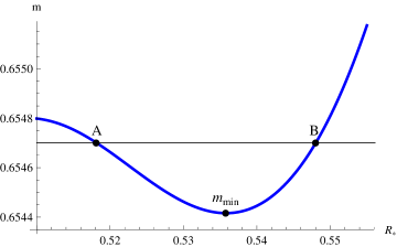
Figure 1: The mass of the fundamental matter as a function of $R_{*}$ at the fixed temperature $T=0.22733$. The minimum value of mass is given by $m_{min}=0.654416\ (R_{*min}=0.53575)$.

Our numerical calculation shows that there is no one to one correspondence between mass and $R_{*}$ in the near horizon region. In fact for a fixed value of mass there are two possible solutions (see points A and B in the Fig. 1) and the question is that between these two points which probe brane configuration is more stable. Since the system is in equilibrium, the configuration with lower energy is more stable. To compare the energies one needs to find the Hamiltonian which in our case is given by

$$E=\int_{r_{*}}^{\infty}dr{\cal{H}}-{\cal{L}}_{\rm{cont}},$$ (2.10)

where ${\cal{H}}=-{\cal{L}}$. ${\cal{L}}_{\rm{cont}}=L_{1}+L_{2}+L_{3}$ represents the counterterms that renormalize the divergence at the boundary and $L_{1}$, $L_{2}$ and $L_{3}$ are explicitly introduced in [13, 12]. It is found from our numerical analysis that the configuration corresponding to point B has lower energy and as a result the solution with larger $R_{*}$ is the physical one. Similarly other points on the right part of the curve has lower energy in comparison with the corresponding points on the left side that have the same mass. Therefore for the physical configurations, $R_{*}$ is always larger than $R_{*min}$ corresponding to $m_{min}$.

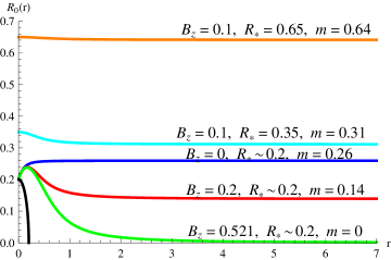
Figure 2: Behaviour of the function $R_{0}(r)$ at the fixed temperature $T=0.0900316$ for different values of the magnetic field.

When the magnetic field is non-zero, as it is evidently seen from Fig. 2, the value of the mass decreases as the magnetic field increases. Therefore, at fixed temperature and $R_{\ast}$ an upper limit exists for the magnetic field. For larger values of the magnetic field the mass of the quark becomes negative and the corresponding configurations are not physical [15]. Moreover, we would like to emphasis that when $R_{*}\gg\rho_{h}\sim T$ the embedding solution $R_{0}(r)$ is almost constant (cyan and orange curves in Fig. 2). However, in the near horizon region where $R_{*}\gtrsim\rho_{h}$, meaning that the tip of the brane is close to the horizon, non-trivial solutions exist (blue, red and green curves in Fig. 2).

In the presence of the magnetic field, although the energy of the system is still given by (2.10), the Lagrangian of the counterterms has now an extra term

$${\cal{L}}_{\rm{cont}}=L_{1}+L_{2}+L_{3}+L_{f},$$ (2.11)

where $L_{f}$ has been also introduced in [13, 12], explicitly. Our results show that, even in the presence of the magnetic field, for fixed values of mass the solutions with larger $R_{*}$ (i.e. $R_{*}>{R_{*}}_{min}$) have lower energy and therefore are more stable. Different aspects of the probe brane in the presence of the magnetic field have been studied in the literature [13, 12, 14].

3 Thermal Fluctuations and Imaginary Part of the Action

In this section we are interested in studying the effect of a certain class of fluctuations about the ME on the action of the brane. Due to these fluctuations, an imaginary term induces on the action of the probe brane. We will find the general expression for the imaginary part of the action in terms of metric components and external magnetic field.

To compute the effect of the fluctuations on the probe brane action, the starting point is to define the fluctuations as

$$R_{0}(r)\rightarrow R_{0}(r)+\delta R(r),$$ (3.1)

where $R_{0}(r)$ and $\delta R(r)$ denote a ME and fluctuations about it, respectively. $\delta R(r)$ is taken to be small and we also impose the long wavelength condition on the fluctuations meaning $\frac{d(\delta R)}{dr}\rightarrow 0$. As a result it is acceptable to expand the ME around the $r=0$ because the fluctuations have the most contribution around this point. Regarding the second boundary condition ($\dot{R}_{0}(0)=0$), we have

$$R_{0}(r)=R_{*}+\frac{1}{2!}\delta r^{2}\ddot{R}_{0}(0)+\dots,$$ (3.2)

and, using the above equation, it is easy to find

$$\begin{split}P=P(R_{*})&+\frac{1}{2!}\delta r^{2}\ddot{R}_{0}(0)P^{\prime}(R_{*})+P^{\prime}(R_{*})\delta R(0)\cr&+\frac{1}{2}P^{\prime\prime}(R_{*})\delta R(0)^{2}+\dots,\end{split}$$ (3.3)

where ${}^{\prime}=\frac{d}{dR}$ and $P$ has been defined in (2.6a). Similar expansion with (3.3) can be written for $Q$. After substituting (3.3) in the term under the square root in (2.5) we have

$$\sqrt{C_{1}\delta r^{2}+C_{2}},$$ (3.4)

where

$$C_{1} =\frac{\ddot{R}_{0}(0)}{2}\left(2\ddot{R}_{0}(0)Q(R_{*})+P^{\prime}(R_{*})\right),$$ (3.5a)

$$C_{2} =P(R_{*})+\delta R(0)P^{\prime}(R_{*})+\frac{1}{2}\delta R(0)^{2}P^{\prime\prime}(R_{*}),$$ (3.5b)

up to second order in $\delta r$ and $\delta R$.

Since we are working in the classical gravity regime, the saddle point approximation for $\delta R$ can be used to find the main contribution of the thermal fluctuations to the action. Therefore, the value of (3.5b) can be analytically computed in this approximation. Using (3.4) and (3.5b) it is easy to obtain

$$\delta R(0)=-\frac{P^{\prime}(R_{*})}{P^{\prime\prime}(R_{*})},$$ (3.6)

and by substituting (3.6) into (3.5), we finally have

$$C_{2}=P(R_{*})-\frac{P^{\prime}(R_{*})^{2}}{2P^{\prime\prime}(R_{*})}.$$ (3.7)

The imaginary part of the action, if any, arises form (3.4). We can not discuss about the sign of $C_{1}$ and $C_{2}$ generally. Therefore, regarding our numerical calculation, we assume that $C_{1}>0$ and $C_{2}<0$ in a specific region of $R_{*}$. Hence the expression under the square root in (3.4) is negative in the following region

$$\begin{split}0<\delta r<\delta r_{c}&=\sqrt{\frac{-C_{2}}{C_{1}}}\cr&=\left[\frac{-2\Big{(}2P^{\prime\prime}(R_{*})P(R_{*})-P^{\prime}(R_{*})^{2}\Big{)}}{\ddot{R}_{0}(0)P^{\prime\prime}(R_{*})\left(2\ddot{R}_{0}(0)Q(R_{*})+P^{\prime}(R_{*})\right)}\right]^{\frac{1}{2}},\end{split}$$ (3.8)

and in this region, in the lowest order, the imaginary part is consequently given by

$${\rm{Im}}S\sim\int_{0}^{\delta r_{c}}d(\delta r)\ e^{-\phi(R_{*})}(g_{ss}^{3}g_{rr})^{\frac{1}{2}}_{R=R_{*}}\sqrt{C_{1}\delta r^{2}+C_{2}}.$$ (3.9)

Equations (3.5)-(3.9) are quite general and applicable to any arbitrary background. In a specified background, for instance $AdS_{5}\times S^{5}$, for each value of $R_{*}$ one can find a ME, $R_{0}(r)$. Using $R_{*}$ and the second derivative of $R_{0}(r)$ at $r=0$, the functions $C_{1}$, $C_{2}$ and consequently, from (3.9), ${\rm{Im}}S$ are determined specifically.

It is worth noting that $C_{2}$ must be negative in the near horizon region in order for the action to gain an imaginary part. Our numerical computations for AdS background, (2.9), show that this requirement is established just when the background is at ”finite temperature”. It is obvious from Fig. 3 that $C_{2}\geq 0$ at zero temperature which means that the action will not develop an imaginary part. This is the reason that we use the expression of ”thermal fluctuations” for the mentioned class of fluctuations.

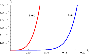
Figure 3: Dependence of $C_{2}$ on $R_{*}$ at zero temperature in the presence and absence of the magnetic field.

3.1 More on Thermal Fluctuation

Before giving a prescription for calculating thermal width, we would like to mention a few points about thermal fluctuations which are compatible with our physical intuition (see Fig. 4).

• As it was obtained in (3.6), in our calculations the fluctuations can be written in terms of the metric components and the external magnetic field. In $AdS_{5}\times S^{5}$ background our numerical computations display that the value of the thermal fluctuations is negative (in a region of $R_{*}$ with $C_{2}<0$).

• Raising the temperature the fluctuations, needed to make the brane configuration unstable, become smaller at fixed mass. The reason is simply that the tip of the probe brane becomes closer to the horizon for higher temperature.

• At fixed temperature, in order to have an imaginary term in the brane action, the absolute value of the fluctuations increases for larger values of mass. It seems reasonable because for larger masses the tip of the probe brane goes further away from the horizon.

• If we attempt to gain an adequate function describing the thermal fluctuations in terms of mass, the best fit we find is

  $$\delta R(0)=\frac{\alpha_{1}+\alpha_{2}m^{2}+\alpha_{3}m^{4}}{\alpha_{4}+\alpha_{5}m^{2}+\alpha_{6}m^{4}},$$ (3.10)

  where $\alpha$s are temperature dependent coefficients. Using various computational software programs, such as Mathematica, the coefficients can be found and the resulting function has been shown by blue curve in Fig. 4(left). Since the values of $\alpha$s are not illuminating, we did not write them here explicitly.

• In Fig. 4(right) the fluctuations in terms of mass has been plotted in the presence of the external magnetic field. It is obvious that for non-zero magnetic field the fluctuations have to increase in order to make the configuration unstable. This happens because the magnetic field increases the effective tension of the probe brane and the brane resists more against the deformation.

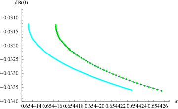
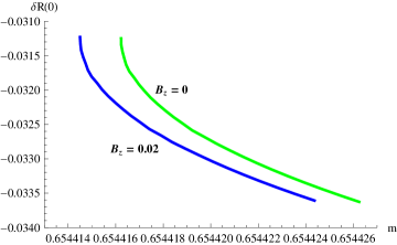
Figure 4: The above figures have been plotted between critical mass(see after (4.1) for definition) and $m_{min}$.
Left: Thermal fluctuations in terms of mass for $T=0.22733$(green) and $T=0.227329$(cyan). The blue curve shows the fitted function (3.10).
Right: Thermal fluctuations in terms of mass for non-zero magnetic field and $T=0.22733$.

4 Holographic Thermal Width

From the gauge/gravity duality point of view, the dissociation of the mesons is identified with a first order phase transition between a ME and a BE. Holographic calculation shows that the dissociation temperature $T_{diss}$ is proportional to the bare mass of the quark $T_{diss}\sim m_{q}/\sqrt{\lambda}$ [9, 2]. Notice that the phase transition of the probe brane’s shape means that some of the MEs turn out to be unstable in the near horizon region.

As it was discussed in (2.7) for the MEs, the mass of the fundamental matter is proportional to the asymptotic value of the $R_{0}(r)$,

$$m=\lim_{r\rightarrow\infty}R_{0}(r).$$ (4.1)

In the following subsections at fixed temperature we will find a critical mass $m_{c}$ where for available mass smaller than $m_{c}$ an imaginary term contributes to the action of the probe branes. In other words, it indicates that the corresponding MEs are not stable for $m_{min}<m<m_{c}$ and a phase transition (first order) from MEs to BEs may occur ($m_{min}$ was introduced in Fig. 1) . In the gauge theory when the mass of the quark is less than $m_{c}$ the quarkonium mesons are unstable. Such mesons are disappeared (melted) into the plasma and a thermal quark is created from the medium. Therefore one can define a thermal width for the quarkonia. We consider the imaginary part of the action of the probe brane proportional to the thermal width of the quarkonium mesons in the gauge theory

$$\Gamma\sim{\rm{Im}}S.$$ (4.2)

Obtaining the imaginary part of the action of the probe brane from (3.9), we aim to compute the thermal width of quarkonia in the ${{\cal{N}}=4}$ gauge theory. In the following subsections we like to study the behavior of the thermal width in the absence and in the presence of a magnetic field.

4.1 Zero Magnetic Field

We start with the metric (2.9) corresponding to AdS-Schwarzschild background and we also set the magnetic field to zero. The dependence of the functions $C_{1}$ and $C_{2}$ on $R_{*}$ and $\rho_{h}$ is given by

$$\begin{split}C_{1}&=\frac{\ddot{R}_{0}(0)(R_{*}^{8}-\rho_{h}^{8})\left(4(R_{*}^{8}+\rho_{h}^{8})+\ddot{R}_{0}(0)R_{*}(R_{*}^{8}-\rho_{h}^{8})\right)}{R_{*}^{9}},\cr C_{2}&=\frac{(3R_{*}^{8}-5\rho_{h}^{8})(R_{*}^{8}-\rho_{h}^{8})^{3}}{R_{*}^{8}(7R_{*}^{16}+9\rho_{h}^{16})},\end{split}$$ (4.3)

and for fixed temperatures they are shown in Fig. 5. As it is clearly seen from this figure, $C_{1}$ is always positive and our numerical calculation approves this behavior for different temperatures. But $C_{2}$ becomes negative in the near horizon region and according to our results in the previous section in this region an imaginary part contributes to the action of the probe brane. Consequently the corresponding mesons in the QGP become unstable. Since the Dilaton field is constant in this background, $\eqref{act3}$ and $\eqref{ImS}$ lead to

$$\begin{split}\Gamma&\sim\int_{0}^{\delta r_{c}}d(\delta r)~{}\delta r^{3}\sqrt{C_{1}\delta r^{2}+C_{2}},\cr&\sim\frac{2(-C_{2})^{\frac{5}{2}}}{15R_{*}^{4}C_{1}^{2}}.\end{split}$$ (4.4)

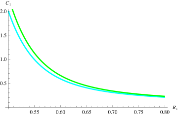
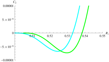
Figure 5: $C_{1}$ in terms of $R_{*}$ (Left) and $C_{2}$ in terms of $R_{*}$ (Right) for two different temperatures $T=0.22508$ and $0.22733$ corresponding to cyan and green curves, respectively.

As it was indicated in the previous section, there is no one to one correspondence between mass and $R_{*}$ in the near horizon region. Hence in order to plot the thermal width in terms of the mass, one should select the favorable configurations whose $R_{*}$s are larger than ${R_{*}}_{min}$ (see Fig. 1). At fixed temperature, the behavior of the thermal width with respect to the mass has been plotted in Fig. 6. We clearly observe that for each value of the temperature there is a critical value for the mass $m_{c}$ where for $m>m_{c}$ the action of the probe brane remains real and as a result the corresponding mesons in the plasma are stable. In order to find the value of the critical mass, we set $C_{2}$ to zero which leads to a value for $R_{*}$ named ${R_{*}}_{c}$. Solving the equation of motion for the $R(r)$ with $R_{*}={R_{*}}_{c}$, the asymptotic value of the resulting ME gives the value of the critical mass. In other words, the critical value for the mass comes from the minimum value of $R_{*}$ for which the action is real. Moreover, the comparison between plots for different temperatures in Fig. 6 shows that the critical mass increases by raising the temperature as it is expected. Fig. 6 also indicates that for $m<m_{c}$ the value of the thermal width increases up to a maximum value $\Gamma_{max}$ which corresponds to the minimum value of the mass, $m_{min}$. The mentioned fact in the literature that the thermal width increases with temperature [2] is shown in Fig 6 (Right). It is obvious that for a fixed value of mass, for example $m_{min}$, the thermal width corresponding to the higher temperature (green plot) has larger value.

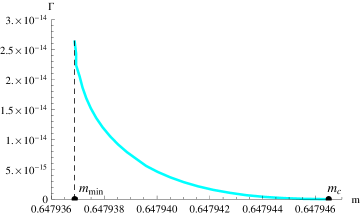
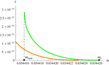
Figure 6: Dependence of the thermal width on the mass. Left: $T=0.22508$. Right: $T=0.22733$ and $0.227329$ corresponding to green and orange curves, respectively.

At sufficiently large $m$ (compared with temperature) the MEs are thermodynamically favorable. By decreasing the mass, there is a critical mass $m_{c}$ at which the action of the probe brane becomes imaginary and therefore the phase transition between a ME and a BE may happen. The value of the critical mass is reported as $m_{c}\sim 0.46\sqrt{\lambda}T$ (for example see [23]). In our units $\lambda=(2\pi)^{2}$ and for $T=0.22508(0.22733)$ the critical mass is $m_{c}\sim 0.6505(0.6570)$. Interestingly, our result (see Fig. 6) shows that the value for the critical mass is $0.647947(0.654426)$ which is in agreement with the reported result.

It is also realized from Fig. 6 that the critical mass varies with the temperature. To see this variation we have plotted the critical mass in terms of the temperature in Fig. 7 that clearly shows the linear increase of $m_{c}$ with respect to the temperature. Again our result is in agreement with proportionality between $m_{c}$ and $T$ reported in the literature [23].

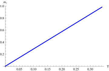
Figure 7: Critical mass in terms of temperature. The plot is fitted with $m_{c}=2.87875\ T$.

In short, we have introduced a new mechanism for the phase transition between a ME and a BE. As we showed thermal fluctuations are responsible for the phase transition in the near horizon region.

Before closing this section, let us discuss a spacial solution for which $R(r)$ is constant. This is the solution when $m\gg T$(or $T=0$). Then, from (4.3), one can find out that $C_{1}$ vanishes and $C_{2}>0$ indicating that the imaginary part of the action disappears. Therefore, the solutions with constant $R(r)$ are stable.

4.2 Non-zero Magnetic field

In the previous subsection we studied the possibility of the appearance of thermal width for quarkonia and its dependence on the mass and the temperature. Now we want to study the same features in the presence of magnetic field. By turning on the magnetic field, according to (2.6a), an extra term appears in the definition of $P$. In the near horizon region, $C_{1}$ and $C_{2}$ are positive and negative, respectively. Since they are too lengthy, we did not write them here. In Fig. 8(left), $C_{2}$ has been plotted in terms of $R_{*}$ at a fixed temperature. Although this figure shows that ${R_{*}}_{c}$, for which $C_{2}$ vanishes, becomes larger in the presence of magnetic field, the critical mass $m_{c}$ decreases as it is shown in Fig. 8(right) in agreement with the result reported in [24]. This behavior can be qualitatively understood from Fig. 2. Similar to the case of zero magnetic field, the thermal width increases as the mass of the quarks decreases.

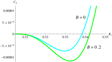
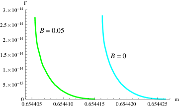
Figure 8: Dependence of $C_{2}$ on $R_{*}$ (Left) and dependence of the thermal width on the mass (Right) for two fixed values of the magnetic field and at the temperature $T=0.22733$.

The critical mass as a function of the temperature is plotted in Fig. 9(left) for fixed values of magnetic field. Unlike the case of zero magnetic field, it shows that the critical mass does not rise linearly with the temperature. The function for critical mass seems to be complicated in the presence of the magnetic field but it may be approximated by the following polynomial

$$m_{c}=T\sum_{n=0}^{5}a_{n}\left(\frac{(2\pi\alpha^{\prime})^{2}B^{2}}{T}\right)^{n}$$ (4.5)

where $a_{0}=2.87875$ and for $B=0.1$:

$$\begin{split}a_{1}=-0.6068,a_{2}=36.6865,a_{3}=-719.758,a_{4}=3202.56,a_{5}=-4496.51,\end{split}$$

and for $B=0.05$:

$$a_{1}=-1.01318,a_{2}=206.215,a_{3}=-12821.7,a_{4}=151035,a_{5}=-528361.$$

In addition, it turns out from Fig. 9(left) that at fixed magnetic field there is a minimum value for the temperature, $T_{c}$, where for $T>T_{c}$ the critical mass is non-zero and a first order phase transition happens. On the other hand, for $T<T_{c}<B_{z}$, the critical mass vanishes and the first order phase transition disappears suggesting that MEs are stable configuration in this region of the temperature. Interestingly, there is a qualitative agreement between our result and [24].

Dependence of the critical mass on the magnetic field is shown in Fig. 9(right) for different fixed values of temperature. It is seen that $m_{c}$ decreases by increasing $B$ which means that in the presence of the external magnetic field the probe brane resists more against the phase transition. From this plot, one may easily guess that

$$m_{c}=m_{0}+m_{1}(2\pi\alpha^{\prime})^{2}B^{2},$$ (4.6)

where for instance, when the temperature is $T=0.23408$, we obtain $m_{c}=0.672972$ and $m_{1}=-0.339937$. Note that there is a maximum value for the magnetic field $B_{max}$ and when $B>B_{max}$ MEs are stable. It is also obvious from the plot that the starting point of $m_{c}$ is grater for the larger values of temperature. It means that by increasing temperature the value of the critical mass below which the configuration becomes unstable, increases.

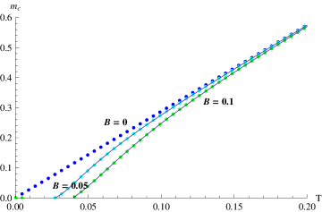
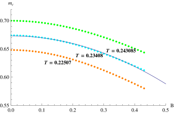
Figure 9: Dependence of $m_{c}$ on the temperature for three values of the magnetic field(left) and on the magnetic field for three values of the temperature(right). The blue curves are fitted functions (4.5) and (4.6) for the left and the right plots, respectively.

5 Summary and Conclusion

In this paper we studied the effect of thermal fluctuations on the instability of a probe D7-brane, being understood by the appearance of an imaginary term in action of the brane that may result in a first order phase transition from Minkowski embedding to black hole embedding. This study is the gravitational dual of meson dissociation in the gauge theory. Therefore we corresponded the imaginary part of the action to the thermal width of quarkonium mesons.

It was seen that there is a critical mass $m_{c}$ above it the thermal width is zero and below it the thermal width increases with mass until it reaches a maximum at an allowed minimum mass, $m_{min}$. Furthermore, $m_{c}$ increases linearly with temperature. As a matter of fact, for higher temperatures the maximum value of the mass, that below it quarkonium mesons dissociate, increases. In other words, since $M_{meson}\sim m_{q}$, it indicates that heavier quarkonia melt in the plasma by increasing the temperature. We also showed that the thermal width increases with temperature for a fixed value of mass.

All the above features had been studied in the presence of the magnetic field, too, and similar results were obtained. The only different and notable points in the latter case are a decrease in $m_{c}$ with increasing the magnetic field and non-linear relation between $m_{c}$ and the temperature. It was seen that in the presence of a non-zero magnetic field there is a minimum value for the temperature, $T_{c}$, that $m_{c}$ is non-zero just for $T>T_{c}$ and for $T<T_{c}$ MEs are stable and accordingly the thermal width is zero.

References

- [1] Quarkonium Working Group Collaboration, N. Brambilla et al., Heavy quarkonium physics, [arXiv:hep-ph/0412158].
- [2] J. Casalderrey-Solana, H. Liu, D. Mateos, K. Rajagopal and U. A. Wiedemann, “Gauge/String Duality, Hot QCD and Heavy Ion Collisions,” [arXiv:1101.0618 [hep-th]].
- [3] B. Alessandro et al. [NA50 Collaboration], “A New measurement of J/psi suppression in Pb-Pb collisions at 158-GeV per nucleon,” Eur. Phys. J. C 39, 335 (2005) [hep-ex/0412036]; R. Arnaldi et al. [NA60 Collaboration], “ production in Indium-Indium collisions at 158- GeV/nucleon,” Conf. Proc. C 060726, 430 (2006) [arXiv:0706.4361 [nucl-ex]]; G. Aad et al. [ATLAS Collaboration], “Measurement of the centrality dependence of yields and observation of Z production in lead-lead collisions with the ATLAS detector at the LHC,” Phys. Lett. B 697, 294 (2011) [arXiv:1012.5419 [hep-ex]]; A. Adare et al. [PHENIX Collaboration], “ Production vs Centrality, Transverse Momentum, and Rapidity in Au+Au Collisions at GeV,” Phys. Rev. Lett. 98, 232301 (2007) [nucl-ex/0611020].
- [4] Y. Burnier, M. Laine and M. Vepsalainen, “Heavy quarkonium in any channel in resummed hot QCD,” JHEP 0801, 043 (2008) [arXiv:0711.1743 [hep-ph]]; Y. Burnier, O. Kaczmarek and A. Rothkopf, “Static quark-antiquark potential in the quark-gluon plasma from lattice QCD,” Phys. Rev. Lett. 114, no. 8, 082001 (2015) [arXiv:1410.2546 [hep-lat]]; L. Thakur, U. Kakade and B. K. Patra, “Dissociation of Quarkonium in a Complex Potential,” Phys. Rev. D 89, no. 9, 094020 (2014) [arXiv:1401.0172 [hep-ph]].
- [5] J. M. Maldacena, “The large N limit of superconformal field theories and supergravity,” Adv. Theor. Math. Phys. 2 (1998) 231 [Int. J. Theor. Phys. 38 (1999) 1113] [arXiv:hep-th/9711200]; S. S. Gubser, I. R. Klebanov and A. M. Polyakov, “Gauge theory correlators from non-critical string theory,” Phys. Lett. B 428 (1998) 105 [arXiv:hep-th/9802109];
- [6] E. Witten, “Anti-de Sitter space and holography,” Adv. Theor. Math. Phys. 2 (1998) 253 [arXiv:hep-th/9802150];
- [7] A. Karch and E. Katz, “Adding flavor to AdS / CFT,” JHEP 0206, 043 (2002) [arXiv:hep-th/0205236].
- [8] J. Erdmenger, N. Evans, I. Kirsch and E. Threlfall, “Mesons in Gauge/Gravity Duals - A Review,” Eur. Phys. J. A 35, 81 (2008) [arXiv:0711.4467 [hep-th]].
- [9] D. Mateos, R. C. Myers and R. M. Thomson, “Holographic phase transitions with fundamental matter,” Phys. Rev. Lett. 97, 091601 (2006), [arXiv:hep-th/0605046]; T. Albash, V. G. Filev, C. V. Johnson and A. Kundu, “A Topology-changing phase transition and the dynamics of flavour,” Phys. Rev. D 77, 066004 (2008), [arXiv:hep-th/0605088];
- [10] D. Mateos, R. C. Myers and R. M. Thomson, “Thermodynamics of the brane,” JHEP 0705, 067 (2007) [arXiv:hep-th/0701132].
- [11] C. Hoyos-Badajoz, K. Landsteiner and S. Montero, “Holographic meson melting,” JHEP 0704, 031 (2007) [arXiv:hep-th/0612169], M. Ali-Akbari and D. Allahbakhshi, “Meson Life Time in the Anisotropic Quark-Gluon Plasma,” [arXiv:1404.5790 [hep-th]].
- [12] C. Hoyos, T. Nishioka and A. O’Bannon, “A Chiral Magnetic Effect from AdS/CFT with Flavor,” JHEP 1110, 084 (2011) [arXiv:1106.4030 [hep-th]].
- [13] A. Karch and A. O’Bannon, “Metallic AdS/CFT,” JHEP 0709, 024 (2007) [arXiv:0705.3870 [hep-th]].
- [14] V. G. Filev and M. Ihl, “Flavoured Large N Gauge Theory on a Compact Space with an External Magnetic Field,” JHEP 1301, 130 (2013) [arXiv:1211.1164 [hep-th]], M. Ammon, V. G. Filev, J. Tarrio and D. Zoakos, “D3/D7 Quark-Gluon Plasma with Magnetically Induced Anisotropy,” JHEP 1209, 039 (2012) [arXiv:1207.1047 [hep-th]], M. Ali-Akbari and H. Ebrahim, “Chiral Symmetry Breaking: To Probe Anisotropy and Magnetic Field in QGP,” Phys. Rev. D 89, 065029 (2014) [arXiv:1309.4715 [hep-th]], M. Ali-Akbari and A. Vahedi, “Non-equilibrium Phase Transition from AdS/CFT,” Nucl. Phys. B 877, 95 (2013) [arXiv:1305.3713 [hep-th]], [arXiv:1305.3713 [hep-th]], M. Ali-Akbari and H. Ebrahim, “Thermalization in External Magnetic Field,” JHEP 1303, 045 (2013) [arXiv:1211.1637 [hep-th]], M. Ali-Akbari and S. F. Taghavi, “-Corrected Chiral Magnetic Effect,” Nucl. Phys. B 872, 127 (2013) [arXiv:1209.5900 [hep-th]].
- [15] J. Babington, J. Erdmenger, N. J. Evans, Z. Guralnik and I. Kirsch, “Chiral symmetry breaking and pions in nonsupersymmetric gauge / gravity duals,” Phys. Rev. D 69, 066007 (2004) [arXiv:hep-th/0306018].
- [16] J. Noronha and A. Dumitru, “Thermal Width of the at Large t’ Hooft Coupling,” Phys. Rev. Lett. 103, 152304 (2009) [arXiv:0907.3062 [hep-th]]; S. I. Finazzo and J. Noronha, “Estimates for the Thermal Width of Heavy Quarkonia in Strongly Coupled Plasmas from Holography,” JHEP 1311, 042 (2013) [arXiv:1306.2613 [hep-th]].
- [17] K. B. Fadafan, D. Giataganas and H. Soltanpanahi, “The Imaginary Part of the Static Potential in Strongly Coupled Anisotropic Plasma,” JHEP 1311, 107 (2013) [arXiv:1306.2929 [hep-th]]. D. Mateos and D. Trancanelli, “Thermodynamics and Instabilities of a Strongly Coupled Anisotropic Plasma,” JHEP 1107, 054 (2011) [arXiv:1106.1637 [hep-th]].
- [18] M. Ali-Akbari, D. Giataganas and Z. Rezaei, “The Imaginary Potential of Heavy Quarkonia Moving in Strongly Coupled Plasma,” [arXiv:1406.1994 [hep-th]].
- [19] K. B. Fadafan and S. K. Tabatabaei, “Thermal Width of Quarkonium from Holography,” Eur. Phys. J. C 74, 2842 (2014) [arXiv:1308.3971 [hep-th]].
- [20] K. Hashimoto and T. Oka, “Vacuum Instability in Electric Fields via AdS/CFT: Euler-Heisenberg Lagrangian and Planckian Thermalization,” JHEP 1310, 116 (2013) [arXiv:1307.7423 [hep-th]].
- [21] N. Brambilla, M. A. Escobedo, J. Ghiglieri and A. Vairo, “Thermal width and quarkonium dissociation by inelastic parton scattering,” JHEP 1305, 130 (2013) [arXiv:1303.6097 [hep-ph]].
- [22] A. Rothkopf, T. Hatsuda and S. Sasaki, “Complex Heavy-Quark Potential at Finite Temperature from Lattice QCD,” Phys. Rev. Lett. 108, 162001 (2012) [arXiv:1108.1579 [hep-lat]].
- [23] C. P. Herzog, A. Karch, P. Kovtun, C. Kozcaz and L. G. Yaffe, “Energy loss of a heavy quark moving through N=4 supermetric Yang-Mills plasma,” JHEP 0607, 013 (2006) [arXiv:hep-th/0605158].
- [24] T. Albash, V. G. Filev, C. V. Johnson and A. Kundu, “Finite temperature large N gauge theory with quarks in an external magnetic field,” JHEP 0807, 080 (2008) [arXiv:0709.1547 [hep-th]].