Signal discovery, limits, and uncertainties with sparse On/Off measurements: an objective Bayesian analysis

Abstract

For decades researchers have studied the On/Off counting problem, where a measured rate consists of two parts. One due to a signal process and another due to a background process, of which both magnitudes are unknown. While most frequentist methods are adequate for large count numbers, they cannot be applied to sparse data. Here I want to present a new objective Bayesian solution that only depends on three parameters: the number of events in the signal region, the number of events in the background region, and the ratio of the exposure for both regions. First, the probability of the hypothesis that the counts are due to background only is derived analytically. Second, the marginalized posterior for the signal parameter is also derived analytically. With this two-step approach it is easy to calculate the signal’s significance, strength, uncertainty, or upper limit in a unified way. The approach is valid without restrictions for any count number including zero and may be widely applied in particle physics, cosmic-ray physics and high-energy astrophysics. In order to demonstrate its performance I apply the method to gamma-ray burst data.

1 Introduction

Typical counting experiments measure a discrete set of events, such as the decay time of a particle. Such data are often (Li & Ma, 1983; Cousins et al., 2008) modeled with the Poisson distribution given by

$$P_{\text{P}}\left(N|\lambda\right)=\frac{e^{-\lambda}\lambda^{N}}{N!}.$$ (1)

This distribution connects the probability to observe N events to a nonnegative number of expected events $\lambda$, derived, for example, from a rate in a fixed time interval or a luminosity and a cross section. The Poisson distribution may be approximated by a Gaussian distribution when measuring many events. But when the data are sparse such an approximation is not good enough. Indeed, in some areas this is often the rule rather than the exception, such as high-energy astrophysics (Loredo, 1992). In this paper a full Bayesian analysis of On/Off data, valid for any count number, is presented.

2 The On/Off Measurement

In the On/Off problem one would like to infer a signal rate in the presence of an imprecisely known background. The measurement consists of the observation of $N_{\text{off}}$ events in a region chosen a priori to be signal free and the observation of $N_{\text{on}}$ events in a region of a potential signal in addition to the background.

The notation comes from astronomy, where telescopes point on and off potential source regions. In particle physics, the off region is taken in some region close to the signal region in the measured parameter (typically called sideband, e.g. Cousins et al., 2008) or without radioactive signal source near the detector.

The ratio of the exposure for both regions $\alpha$ is assumed to be known with negligible uncertainty. In gamma-ray astronomy $\alpha$ is in the most simple cases

$$\alpha=\frac{A_{\text{on}}t_{\text{on}}}{A_{\text{off}}t_{\text{off}}},$$ (2)

where $A$ stands for the size and $t$ for the exposure time of the regions. Berge et al. (2007) illustrate how to generalize Equation 2 for complex acceptances. Given $N_{\text{on}}$, $N_{\text{off}}$, and $\alpha$ the problem is to calculate the evidence for a signal and the posterior distribution of the signal parameter.

Frequentist analyses, based on likelihood ratios and other methods, are widespread in particle physics (Cousins et al., 2008) and in high-energy astrophysics (as promoted by Li & Ma, 1983). However, they often assume normal distributed random numbers and therefore lose their foundation when applying them to low count numbers.

Gillessen & Harney (2005) have proposed a Bayesian solution to the question whether the signal parameter is larger than zero. But they do not account for the alternative, simpler hypotheses asserting that all $N_{\text{on}}$ come from background only, i.e. no source. Therefore the result is an overestimation, as pointed out by Gregory (2005). There exists a Bayesian solution to compute the odds ratio of the two hypotheses (Gregory, 2005), but it adds an arbitrary parameter to the problem, depending on the prior (in particular its upper boundary), which makes the probability statement hard to interpret.

3 Analysis

In this paper an objective Bayesian analysis is presented. This is accomplished by using improper priors as a tool for producing proper posteriors representing our lack of knowledge. Certainly, subjective Bayesian methods can have benefits in particular when a prior opinion is strongly held. One can gain sensitivity by using informative priors that specify prior knowledge precisely, such as a prior source detection or a known background. But objective Bayesian methods should be used when one is interested in “what the data have to say” (Irony & Singpurwalla, 1997).

The analysis presented here follows the recipe outlined by Caldwell & Kröninger (2006) and may be considered an analytical special case. Agostini et al. (2013) applied the recipe in order to analyze and set stringent upper limits on the neutrinoless double beta decay of ⁷⁶Ge. Kashyap et al. (2010) recently presented a similar frequentist method. The analysis is performed in two steps. First, the probability that the observed counts are due to background only is calculated. If this is lower than a previously defined consensus value, the signal is said to be detected. Second, the signal contribution is estimated or an upper limit for the signal is calculated, depending on whether the detection limit has been reached.

3.1 Hypothesis Test

Let $H_{\text{0}}$ denote the null hypothesis that the observed counts are due to background only. The alternative hypothesis $H_{\text{1}}$ is that a signal process contributes to the counts. $H_{\text{1}}$ could be a bad model too, in case of systematic uncertainties. It must be noted that sometimes this is the case when e.g. signal counts leak into the off region. Nevertheless, in the following it is assumed that the systematic uncertainties are negligible and the two model set of exclusive rival hypothesis $\{H_{\text{0}},H_{\text{1}}\}$ is complete. By using Bayes’ theorem one may calculate the conditional probability of $H_{\text{0}}$ as

$$P\left(H_{\text{0}}|N_{\text{on}},N_{\text{off}}\right) = \frac{P\left(N_{\text{on}},N_{\text{off}}|H_{\text{0}}\right)P_{\text{0}}\left(H_{\text{0}}\right)}{P\left(N_{\text{on}},N_{\text{off}}\right)},$$ (3)

where $P\left(N_{\text{on}},N_{\text{off}}|H_{i}\right)$ is the conditional probability to observe the data, given the hypothesis $H_{i}$ and $P_{\text{0}}\left(H_{i}\right)$ is the prior probability for $H_{i}$. For a set of exclusive rival hypothesis such that $\sum_{i}{P(H_{i})}=1$ and $P(H_{i}\land H_{j})=0$ for $i\neq j$, the law of total probability gives

$$P\left(N_{\text{on}},N_{\text{off}}\right)=\sum_{i}P\left(N_{\text{on}},N_{\text{off}}|H_{i}\right)P_{\text{0}}\left(H_{i}\right).$$ (4)

Furthermore, in continuously parametrized models the continuous counterpart of the law of total probability, with sums replaced by integrals, gives

$$P\left(N_{\text{on}},N_{\text{off}}\right)=$$

$$\sum_{i}\int P\left(N_{\text{on}},N_{\text{off}}|\vec{\lambda}_{i},H_{i}\right)P_{\text{0}}\left(\vec{\lambda}_{i}|H_{i}\right)d\vec{\lambda}_{i}P_{\text{0}}\left(H_{i}\right).$$ (5)

The sum is made over the full set of hypotheses $H_{i}$ and the integration with respect to their parameters $\vec{\lambda}_{i}$. By assuming the two hypothesis set $\{H_{\text{0}},H_{\text{1}}\}$ one can write Eqn. 5 in terms of the expected number of signal events $\lambda_{\text{s}}$ and the expected number of background events $\lambda_{\text{bg}}$:

$$P\left(N_{\text{on}},N_{\text{off}}\right)=$$ (6)

$$\int P\left(N_{\text{on}},N_{\text{off}}|\lambda_{\text{bg}},H_{\text{0}}\right)P_{\text{0}}\left(\lambda_{\text{bg}}|H_{\text{0}}\right)d\lambda_{\text{bg}}P_{\text{0}}\left(H_{\text{0}}\right)$$

$$+\int P\left(N_{\text{on}},N_{\text{off}}|\lambda_{\text{s}},\lambda_{\text{bg}},H_{\text{1}}\right)P_{\text{0}}\left(\lambda_{\text{s}},\lambda_{\text{bg}}|H_{\text{1}}\right)d\lambda_{\text{s}}d\lambda_{\text{bg}}$$

$$\times P_{\text{0}}\left(H_{\text{1}}\right).$$

Here, $P\left(N_{\text{on}},N_{\text{off}}|\lambda_{\text{bg}},H_{\text{0}}\right)$ and $P\left(N_{\text{on}},N_{\text{off}}|\lambda_{\text{s}},\lambda_{\text{bg}},H_{\text{1}}\right)$ denote the conditional probabilities to measure the data.

Assuming that the number of signal events (if any) and the number of background events are independent Poisson-distributed random variables with means $\lambda_{\text{s}}$ and $\lambda_{\text{bg}}$, the expected number of events in the off region is

$$E\left(N_{\text{off}}\right)=\lambda_{\text{bg}}.$$ (7)

The expected number of events $E\left(N\right)$ in the on region is, assuming the null hypothesis $H_{\text{0}}$

$$E\left(N_{\text{on}}\right)=\alpha\lambda_{\text{bg}},$$ (8)

or assuming $H_{\text{1}}$

$$E\left(N_{\text{on}}\right)=\lambda_{\text{s}}+\alpha\lambda_{\text{bg}}.$$ (9)

This yields for the conditional probabilities to measure the data or likelihoods

$$P\left(N_{\text{on}},N_{\text{off}}|\lambda_{\text{bg}},H_{\text{0}}\right)=$$

$$P_{\text{P}}\left(N_{\text{on}}|\alpha\lambda_{\text{bg}}\right)P_{\text{P}}\left(N_{\text{off}}|\lambda_{\text{bg}}\right),$$ (10)

and

$$P\left(N_{\text{on}},N_{\text{off}}|\lambda_{\text{s}},\lambda_{\text{bg}},H_{\text{1}}\right)=$$

$$P_{\text{P}}\left(N_{\text{on}}|\lambda_{\text{s}}+\alpha\lambda_{\text{bg}}\right)P_{\text{P}}\left(N_{\text{off}}|\lambda_{\text{bg}}\right).$$ (11)

The priors $P_{\text{0}}\left(\lambda_{\text{bg}}|H_{\text{0}}\right)$ and $P_{\text{0}}\left(\lambda_{\text{s}},\lambda_{\text{bg}}|H_{\text{1}}\right)$ are chosen according to Jeffreys’s rule (see Jeffreys, 1961; Beringer et al., 2012)

$$P_{\text{0}}\left(\vec{\lambda}_{i}|H_{i}\right) \propto \sqrt{\det\left[I\left(\vec{\lambda}_{i}|H_{i}\right)\right]},$$ (12)

$$I_{kl}\left(\vec{\lambda}_{i}|H_{i}\right) = -E\left[\frac{\partial^{2}\ln\,L\left(N_{\text{on}},N_{\text{off}}|\vec{\lambda}_{i},H_{i}\right)}{\partial\lambda_{k}\partial\lambda_{l}}\right],$$ (13)

where $I_{kl}$ denotes the Fisher information matrix, $L$ the likelihood function (either Eqn. 10 or 11), $E$ the expectation value with respect to the model with index $i$ and $\vec{\lambda}_{i}$ its parameter vector. In Appendix A I show that

$$P_{\text{0}}\left(\lambda_{\text{bg}}|H_{\text{0}}\right) \propto \sqrt{\frac{1+\alpha}{\lambda_{\text{bg}}}},$$ (14)

$$P_{\text{0}}\left(\lambda_{\text{s}},\lambda_{\text{bg}}|H_{\text{1}}\right) \propto \sqrt{\frac{1}{\lambda_{\text{bg}}\left(\alpha\lambda_{\text{bg}}+\lambda_{\text{s}}\right)}}.$$ (15)

The On/Off Jeffreys’s priors are improper, i.e. integrate to infinity over the parameter space. There is a debate among statisticians, concerning the use of improper priors in Bayesian model selection (Berger & Pericchi, 2001), as the priors are only specified up to the proportionality constants $c_{0},c_{1}$ which do not cancel out. The probability of $H_{\text{0}}$ to be true given the measured counts is therefore

$$P\left(H_{\text{0}}|N_{\text{on}},N_{\text{off}}\right) = \frac{c_{0}\gamma^{\prime}}{c_{0}\gamma^{\prime}+c_{1}\delta^{\prime}}$$ (16)

$$= \frac{\gamma^{\prime}}{\gamma^{\prime}+\nicefrac{{c_{1}}}{{c_{0}}}\delta^{\prime}},$$ (17)

with

$$\gamma^{\prime}:= \intop_{0}^{\infty}P\left(N_{on},N_{\text{off}}|\lambda_{\text{bg}},H_{\text{0}}\right)$$ (19)

$$\times P_{\text{0}}\left(\lambda_{\text{bg}}|H_{\text{0}}\right)d\lambda_{\text{bg}}P_{\text{0}}\left(H_{\text{0}}\right),$$

$$\delta^{\prime}:= \intop_{0}^{\infty}\intop_{0}^{\infty}P\left(N_{on},N_{off}|\lambda_{\text{s}},\lambda_{\text{bg}},H_{\text{1}}\right)$$

$$\times P_{\text{0}}\left(\lambda_{\text{s}},\lambda_{\text{bg}}|H_{\text{1}}\right)d\lambda_{\text{s}}d\lambda_{\text{bg}}P_{\text{0}}\left(H_{\text{1}}\right).$$

To calculate the analytic outcome of Eqn. 17, the priors for the hypothesis $P_{\text{0}}\left(H_{\text{0}}\right)$ and $P_{\text{0}}\left(H_{\text{1}}\right)$ have to be identified. Given the lack of prior information to which hypothesis is more likely, they are chosen to be equal

$$P_{\text{0}}\left(H_{\text{0}}\right)=P_{\text{0}}\left(H_{\text{1}}\right)=\frac{1}{2}.$$ (20)

When the model parameter spaces are the same, it is common to set $c_{0}=c_{1}$. In the case that that the two models have differing dimensions, special effort has to be invested, in order to assign a value to $\frac{c_{1}}{c_{0}}$, based on extrinsic arguments (Berger & Pericchi, 2001). Therefore, imagine no counts in either region. This means no signal was observed, which means the signal hypothesis $H_{\text{1}}$ can not become more likely

$$P\left(H_{\text{0}}|0,0\right)\geq P_{\text{0}}\left(H_{\text{0}}\right).$$ (21)

This is a limit on the posterior model probability, that can be used as the basis of a robust Bayesian analysis (Berger et al., 1994). In particular I argue that when no counts are observed, the probability for either model stays the same and therefore equality holds in Eqn. 21. The approach leads to the determination of the fraction $\frac{c_{1}}{c_{0}}$ via the equation

$$\frac{c_{1}}{c_{0}} = \frac{\gamma^{\prime}}{\delta^{\prime}}|_{N_{\text{on}},N_{\text{off}}=0}.$$ (22)

The evaluation of Eqn. 17 together with Eqn. 22 may be found in Appendix B. Altogether the probability of $H_{\text{0}}$ being true, given $N_{\text{on}}$ and $N_{\text{off}}$, is

$$P\left(H_{\text{0}}|N_{\text{on}},N_{\text{off}}\right)=\frac{\gamma}{\gamma+\nicefrac{{c_{1}}}{{c_{0}}}\delta},$$ (23)

where $\gamma$ and $\delta$ are defined in terms of the Gamma function $\Gamma\left(x\right)$ and the hypergeometric function ${}_{2}\operatorname{F}_{1}\left(a,b;c;z\right)$

$$\gamma := \left(1+2N_{\text{off}}\right)\alpha^{\nicefrac{{1}}{{2}}+N_{\text{on}}+N_{\text{off}}}$$

$$\times\Gamma\left(\nicefrac{{1}}{{2}}+N_{\text{on}}+N_{\text{off}}\right),$$

$$\delta := 2\left(1+\alpha\right)^{N_{\text{on}}+N_{\text{off}}}\Gamma\left(1+N_{\text{on}}+N_{\text{off}}\right)$$

$$\times_{2}\operatorname{F}_{1}\left(\nicefrac{{1}}{{2}}+N_{\text{off}},1+N_{\text{on}}+N_{\text{off}};\nicefrac{{3}}{{2}}+N_{\text{off}};-\nicefrac{{1}}{{\alpha}}\right),$$

$$\frac{c_{1}}{c_{0}} = \frac{\sqrt{\pi}}{2\arctan\left(\nicefrac{{1}}{{\sqrt{\alpha}}}\right)}.$$ (26)

Equation 23 is, however, not restricted to small count numbers and can, with current PCs and numerical tools like Mathematica, be easily calculated up to thousands of counts.

3.2 Signal Detection

A signal detection based on Eqn. 23 may be claimed when the resulting probability of the null hypothesis $H_{\text{0}}$ is low. In high-energy astrophysics, the consensus (Li & Ma, 1983; Abdo et al., 2009) p value for a source discovery is $p=5.7\times 10^{-7}$, corresponding to a 5$\sigma$ measurement. Scientists frequently use lower thresholds for the detection of known sources. However, this number value is used in this paper for the probability of $H_{\text{0}}$ as source detection criterion.

One must keep in mind that these are two completely different quantities: a probability of a model, and a frequency of an outcome. $P\left(H_{\text{0}}|N_{\text{on}},N_{\text{off}}\right)$ explicitly weighs alternative models, while the frequentist result does not.

That said, and with the help of the inverse error function $\operatorname{erf}^{-1}(x)$, the Bayesian significance $S_{\text{b}}$ is introduced, defined as ”if the probability were normal distributed, it would correspond to a $S_{\text{b}}$ standard deviation measurement“:

$$S_{\text{b}}=\sqrt{2}\operatorname{erf}^{-1}\left[1-P\left(H_{\text{0}}|N_{\text{on}},N_{\text{off}}\right)\right].$$ (27)

Using the above equation, it is easy to compare detection or discovery claims with different methods and thresholds, as shown in Sec. 4.

3.3 Signal Strength

If the counted events lead to a detection, the signal parameter strength can be estimated. In other words, it is safe to assume hypothesis $H_{\text{1}}$. The conditional probability of the signal and the background parameters $\lambda_{\text{s}}$ and $\lambda_{\text{bg}}$ may then be calculated from Bayes’ law:

$$P\left(\lambda_{\text{s}},\lambda_{\text{bg}}|N_{\text{on}},N_{\text{off}},H_{\text{1}}\right)=$$ (28)

$$\frac{P\left(N_{\text{on}},N_{\text{off}}|\lambda_{\text{s}},\lambda_{\text{bg}},H_{\text{1}}\right)P_{\text{0}}\left(\lambda_{\text{s}},\lambda_{\text{bg}}|H_{\text{1}}\right)}{\int_{0}^{\infty}\int_{0}^{\infty}P\left(N_{\text{on}},N_{\text{off}}|\lambda_{\text{s}},\lambda_{\text{bg}},H_{\text{1}}\right)P_{\text{0}}\left(\lambda_{\text{s}},\lambda_{\text{bg}}|H_{\text{1}}\right)d\lambda_{\text{s}}d\lambda_{\text{bg}}}.$$

Given the data, one would like to infer the signal $\lambda_{\text{s}}$ without reference to $\lambda_{\text{bg}}$ but fully accounting for the uncertainty on $\lambda_{\text{bg}}$. This can be done by marginalizing over the nuisance parameter $\lambda_{\text{bg}}$:

$$P\left(\lambda_{\text{s}}|N_{\text{on}},N_{\text{off}},H_{\text{1}}\right)=\int_{0}^{\infty}P\left(\lambda_{\text{s}},\lambda_{\text{bg}}|N_{\text{on}},N_{\text{off}},H_{\text{1}}\right)d\lambda_{\text{bg}}.$$ (29)

Equation 29 can be analytically calculated using Eqn. 11, 15, and the results from Appendix B, which is done in Appendix C. The improper prior is acceptable because the proportionality constant $c_{1}$ cancels and the posterior is proper. The result may be expressed in terms of three functions, namely the Poisson distribution $P_{\text{P}}\left(N|\lambda\right)$, the regularized hypergeometric function ${}_{2}\tilde{\operatorname{F}}_{1}\left(a,b;c;z\right)=\nicefrac{{{}_{2}\operatorname{F}_{1}\left(a,b;c;z\right)}}{{\Gamma\left(c\right)}}$, and the Tricomi confluent hypergeometric function $\operatorname{U}\left(a,b,z\right)$:

$$P\left(\lambda_{\text{s}}|N_{\text{on}},N_{\text{off}},H_{\text{1}}\right)=P_{\text{P}}\left(N_{\text{on}}+N_{\text{off}}|\lambda_{\text{s}}\right)$$ (30)

$$\times\frac{\operatorname{U}\left[\nicefrac{{1}}{{2}}+N_{\text{off}},1+N_{\text{off}}+N_{\text{on}},\left(1+\nicefrac{{1}}{{\alpha}}\right)\lambda_{\text{s}}\right]}{{}_{2}\tilde{\operatorname{F}}_{1}\left(\nicefrac{{1}}{{2}}+N_{\text{off}},1+N_{\text{off}}+N_{\text{on}};\nicefrac{{3}}{{2}}+N_{\text{off}};-\nicefrac{{1}}{{\alpha}}\right)}.$$

This posterior contains the full information. In order to quote numbers one may take the mode $\lambda_{\text{s}}^{*}$, which is the value of $\lambda_{\text{s}}$ that maximizes the posterior distribution $P\left(\lambda_{\text{s}}|N_{\text{on}},N_{\text{off}},H_{\text{1}}\right)$, as signal estimator. The error on the quoted signal can be evaluated from the cumulative distribution function. For instance to get the smallest Bayesian interval (also known as Highest Posterior Density interval or HPD) containing the signal parameter with $68\%$ probability one can solve

$$0.68=\int_{\lambda_{\text{min}}}^{\lambda_{\text{max}}}P\left(\lambda_{\text{s}}|N_{\text{on}},N_{\text{off}},H_{\text{1}}\right)d\lambda_{\text{s}},$$ (31)

together with the constraint

$$P\left(\lambda_{\text{min}}|N_{\text{on}},N_{\text{off}},H_{\text{1}}\right)=P\left(\lambda_{\text{max}}|N_{\text{on}},N_{\text{off}},H_{\text{1}}\right),$$ (32)

numerically for $\lambda_{\text{min}}$ and $\lambda_{\text{max}}$. The final result may be quoted as

$$\lambda_{\text{s}}=\lambda_{\text{s}-(\lambda_{\text{s}}^{*}-\lambda_{\text{min}})}^{*+(\lambda_{\text{max}}-\lambda_{\text{s}}^{*})}.$$ (33)

3.4 Signal Upper Limit

If the data show no significant detection, an upper limit on the signal parameter may be calculated, assuming that the signal is there (i.e. $H_{\text{1}}$ is true) but too weak to be measured. For example a $99\%$ probability limit $\lambda_{99}$ on the signal parameter $\lambda_{\text{s}}$ is calculated by solving

$$\intop_{0}^{\lambda_{99}}P\left(\lambda_{\text{s}}|N_{\text{on}},N_{\text{off}},H_{\text{1}}\right)d\lambda_{\text{s}}=0.99.$$ (34)

This result comes naturally in a Bayesian approach of the problem but is hard to calculate in a frequentist approach. In particular frequentists struggle with the marginalization of the problem and with special cases at the border of the parameter space, all of which lead to ad hoc adjustments without theoretical justification (Rolke et al., 2005). The only practical remedy comes from Monte Carlo studies that in fact such limits with adjustments have (at least) the claimed frequentist coverage. In this Bayesian approach, all possible values in the parameter space are dealt with in a uniform way, no matter if zero counts or thousands of counts. The signal upper limit result is in particular interesting for $N_{\text{on}}=N_{\text{off}}=0$. It underlines that measuring zero is different from not measuring at all, hence valid limits can be derived. Importantly the estimates are always physically meaningful (i.e. positive $\lambda_{\text{s}}^{*},\lambda_{min},\lambda_{max},\lambda_{99},...$ ).

4 Validation

Jeffreys’s prior is constructed by a formal rule (Jeffreys, 1961) and motivated by the requirement for invariance under one-to-one transforms. However this is not the only possible choice and, when data are sparse, the choice of the prior is important. In order to validate that it is a reasonable choice I compare it to the prior from Gregory (2005), the frequentist solution from Li & Ma (1983), and to a simulation.

4.1 Model Comparison

For the On/Off problem one alternative with informative flat priors was presented by Gregory (2005). The hypothesis test is, in this case, dependent on the prior signal upper boundary $\lambda_{\textrm{smax}}$ in addition to $N_{\textrm{on}}$, $N_{\textrm{off}}$ and $\alpha$. Therefore reasonable assumptions on the signal upper boundary $\lambda_{\textrm{smax}}$ have to be made, in order to compare Eqn. 14.24, Gregory (2005) with Eqn. 23. The signal posteriors however can be compared directly as they depend only on the three initial parameters in both cases.

Figure 1: Comparison of the On/Off hypothesis test with Jeffreys’s and Gregory’s priors for low and large count numbers. In a) the null hypothesis posterior probability is shown as a function of $N_{\text{on}}$ in the low counts regime. b) shows the same but using the nonlinear Bayesian significance scale Eqn. 27. In c) the limiting curves for which $N_{\text{on}}:S_{\text{b}}\geq 3$ or $S_{\text{b}}\geq 5$ are shown. d) shows a comparison in the large counts regime and additionally Li & Ma (1983), Eqn. 17.

Figure 2: Comparison of the signal posteriors with Jeffreys’s and Gregory’s priors. a) shows a comparison for low count numbers. b) shows a comparison for high count numbers and shows additionally a normal distribution with mean Eqn. 35 and variance Eqn. 36

The hypothesis test comparison is shown in Fig. 1. Fig. 1a, 1b, and 1c show the situation for a typical low count case with $\alpha=0.2$ and an assumed $\lambda_{\textrm{smax}}=22$ such that a signal detection with that strength would be without any doubt. Gregory’s prior shows a similar behavior as the Jeffreys’s prior, but is slightly shifted towards higher probabilities for the null hypothesis $P\left(H_{\text{0}}|N_{\text{on}},N_{\text{off}}\right)$ or lower significance $S_{\textrm{b}}$ (Eqn. 27). In Fig. 1c one can see the limiting curve for which $N_{\textrm{on}}$, given $N_{\textrm{off}}$, the significance $S_{\textrm{b}}$ is $\geq 3$ or $\geq 5$. This shows that, when it comes to decision making in the low-count regime, both models are mostly within one count from another.

Figure 1d shows a comparison of the different priors for high count numbers with $\alpha=0.2$, $N_{\textrm{off}}=300$ and $\lambda_{\textrm{smax}}=170$. Additionally, the methods are compared to the frequentist result of Li & Ma (1983), Eqn. 17. Both methods appear to converge on Li & Ma’s result for large count numbers, but Jeffreys’s prior gives a closer approximation. From a physical point of view one could argue that for $N_{\textrm{on}}\sim\alpha N_{\textrm{on}}$, $P\left(H_{\text{0}}|N_{\text{on}},N_{\text{off}}\right)$ should be close to the prior model probability $P_{0}\left(H_{\text{0}}\right)=0.5$ because any one $N_{\textrm{on}}$ more should increase the probability for the signal hypothesis $H_{1}$ and any $N_{\textrm{on}}$ less should decrease it. Numerically it seems that this is the case for Jeffreys’s prior, but not for Gregory’s prior.

When comparing the signal posterior, Jeffrey’s and Gregory’s priors agree well. Fig. 2a shows a comparison of the two methods for low count numbers with $\alpha=0.2$, $N_{\textrm{off}}=5$. The differences in the signal posterior are marginal. For high count numbers, as shown in Fig. 2b with $\alpha=0.2$, $N_{\textrm{off}}=80$, both methods converge quickly to the to the classical result of a normal distribution with

$$E(\lambda_{\textrm{s}}) =N_{\textrm{on}}-\alpha N_{\textrm{off}}$$ (35)

$$Var(\lambda_{\textrm{s}}) =N_{\textrm{on}}+\alpha^{2}N_{\textrm{off}}.$$ (36)

However, because of the subtraction and when $N_{\textrm{on}}\sim\alpha N_{\textrm{on}}$ the normal distribution can include negative values for the signal confidence region. This problem is resolved using the Bayesian methods.

Overall the results are comparable and show that the results obtained by Jeffreys’s prior are sensible. They behave well in all test-case examples, in particular at $N_{\textrm{on}}\sim\alpha N_{\textrm{on}}$, and converge to the other results for high count numbers.

4.2 Simulations

To further verify the method developed in this paper, the hypothesis test and the maximum signal posterior are calculated for a simulated set of observations. First, one thousand $N_{\textrm{on}}$ and $N_{\textrm{off}}$ are drawn randomly from two Poisson distributions with means of Eqn. 7 and Eqn. 9. Second, the developed methods are applied to the simulation, as well as Li & Ma’s method for the hypothesis test and a direct background subtraction (Eqn. 35) for the signal strength. Then, the results of these methods are compared to one another and to the true parameters. These are $\lambda_{\textrm{bg}}=300$ for the background strength and $\lambda_{\textrm{s}}=50$ for the signal strength. The ratio of exposure $\alpha$ is 1/5.

Figure 3: Simulation results of the analysis, in comparison to Li & Ma and direct background subtraction.

Figure 3a shows the hypothesis test simulation results. Li & Ma’s test statistic shows a small systematic shift in comparison to the Bayesian significance (Eqn. 27) in agreement with the results from Sec. 4.1. In Fig. 3b the signal strength comparison is shown. The parameter $\lambda_{\text{s}}^{*}$ is first calculated as the maximum of the marginalized posterior (Eqn. 30) and second with direct background subtraction. Both methods agree well and can reconstruct the true signal parameter $\lambda_{\textrm{s}}=50$ with similar errors.

5 Application: Gamma-Ray Bursts

Gamma-ray bursts (GRB) are extraterrestrial flashes of gamma-rays, lasting only few seconds mostly. One interesting question is whether gamma-ray bursts produce very high energy ($>100$GeV) gamma-rays, as proposed by some theories (e.g. Abdo et al., 2009). Because of their duration and fluence, gamma-ray satellites and Cherenkov telescopes measure only few events during the flare itself, or shortly thereafter. In Tab. 5 data from 12 gamma-ray burst observations, made by the space based Fermi Large Area Telescope (Fermi-LAT) and the ground based VERITAS Cherenkov telescope, are compiled.

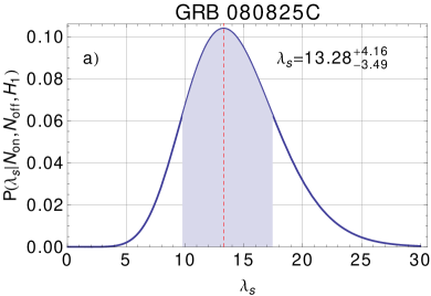
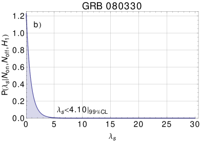
Figure 4: Comparison of the marginal signal parameter $\lambda_{\text{s}}$ posterior distribution for two gamma-ray bursts. In a), GRB 080825C, a source is detected and the signal parameter estimate and its smallest $68\%$ credibility interval is calculated. In b) an upper limit is calculated for GRB 080330 where no on event was measured.

Table 1: Low count gamma-ray burst data

GRB	$N_{\text{on}}$	$N_{\text{off}}$	$\alpha$	$S_{\text{lm}}$	$P(H_{\text{0}}|N_{\text{on}},N_{\text{off}})$	$S_{\text{b}}$	$\lambda_{\text{s}}$	$\lambda_{99}$	$\lambda_{\textrm{Ref.}}$	$\lambda_{99}^{\textrm{Rolke}}$	Reference
070419A	2	14	0.057	…	0.28	1.09	…	6.88	…	7.34	1
070521	3	113	0.057	…	0.72	0.36	…	6.12	…	3.52	1
070612B	3	21	0.066	…	0.26	1.12	…	8.00	…	8.54	1
080310	3	23	0.128	…	0.51	0.66	…	7.16	…	7.08	1
080330	0	15	0.123	…	0.70	0.39	…	4.10	…	2.40	1
080604	2	40	0.063	…	0.58	0.55	…	6.12	…	5.66	1
080607	4	16	0.112	…	0.21	1.27	…	9.17	…	9.83	1
080825C	15	19	0.063	6.4	9.66E-10	6.11	$\mathbf{13.28_{-3.49}^{+4.16}}$	…	13.7	…	2
081024A	1	7	0.142	…	0.50	0.67	…	5.29	…	5.19	1
090418A	3	16	0.123	…	0.37	0.89	…	7.64	…	8.01	1
090429B	2	7	0.106	…	0.26	1.13	…	6.92	…	7.41	1
090515	4	24	0.126	…	0.41	0.83	…	8.34	…	8.66	1

Note. — Table 5 shows low count gamma-ray burst data where either or both of $N_{\text{on}}$ or $N_{\text{off}}$ are $\leq 15$. Only GRB 080825C was detected with a high significance. Its reference source strength $\lambda_{\text{Ref.}}$ is given in Abdo et al. (2009). All calculated values are in bold. The ratio of exposure $\alpha$ is calculated according to Acciari et al. (2011). The $\alpha$ values are then used for calculating Rolke’s upper limit $\lambda_{99}^{\textrm{Rolke}}$.

References. — (1) Acciari et al. (2011), (2) Abdo et al. (2009)

Due to the difficulty of the detection, reporting of those events is usually an upper limit with low statistics. Only for the Fermi-LAT GRB 080825C there was significant evidence to report a discovery. For this gamma-ray burst, the probability of the background-only model $P(H_{\text{0}}|N_{\text{on}},N_{\text{off}})$ is $9.66\times 10^{-10}$ and the gamma-ray burst is therefore detected. The significance expressed on the nonlinear scale (Eqn. 27) is $S_{\text{b}}=6.11$. This is comparable to the Li & Ma result of $S_{\text{lm}}=6.4$.

In the second step, the most likely value of the signal parameter and the smallest $68\%$ credibility interval is calculated. The method is demonstrated in Fig. 4. The result is that $\lambda_{\text{s}}=13.28_{-3.49}^{+4.16}$, which is in good agreement to the published reference of $\lambda_{\text{Ref.}}=13.7$.

In the same figure an observation from the gamma-ray burst GRB 080330, for which discovery cannot be claimed, is shown. For GRB 080330 and all other gamma-ray bursts, the data do not show evidence for a source of gamma-rays. In this case, upper limits $\lambda_{99}$ are calculated. All results are summarized in Table 5 and are compared to the Rolke $99\%$ upper limits $\lambda_{99}^{\textrm{Rolke}}$, which VERITAS used. GRB 080330 is special in the sense that not even one on event was measured. The results are mostly in good agreement but, especially at the border of the parameter space for $N_{\text{on}}\leq\alpha N_{\text{off}}$, also deviate from another and show the limit of Rolke’s method - which are overcome by the Bayesian method.

6 Conclusion

Many particle physicists, cosmic-ray physicists and high-energy astrophysicists struggle with sparse On/Off data. With this new Bayesian method, that overcomes the weaknesses of the presently used methods, it is possible to go down to single count On/Off measurements. Claiming detections, setting credibility intervals, or setting upper limits is unified in a single and consistent method.

Appendix A Jeffreys’s Priors

Calculation of the prior of $\lambda_{\text{bg}}$ in the $H_{\text{0}}$ model:

$$P_{\text{0}}\left(\lambda_{\text{bg}}|H_{\text{0}}\right)=\boldsymbol{(}-\sum_{N_{\text{on}}=0}^{\infty}\sum_{N_{\text{off}}=0}^{\infty}$$

$$\left\{\partial_{\lambda_{\text{bg}}}^{2}\ln\left[P_{\text{P}}\left(N_{\text{on}}|\alpha\lambda_{\text{bg}}\right)P_{\text{P}}\left(N_{\text{off}}|\lambda_{\text{bg}}\right)\right]\right\}$$

$$\times P_{\text{P}}\left(N_{\text{on}}|\alpha\lambda_{\text{bg}}\right)P_{\text{P}}\left(N_{\text{off}}|\lambda_{\text{bg}}\right)\boldsymbol{)}^{\frac{1}{2}}=\sqrt{\frac{1+\alpha}{\lambda_{\text{bg}}}}.$$

Calculation of the prior for $\lambda_{\text{s}}$ and $\lambda_{\text{bg}}$ in the $H_{\text{1}}$ model:

$$I_{s,s}=-\sum_{N_{\text{on}}=0}^{\infty}\sum_{N_{\text{off}}=0}^{\infty}$$

$$\left\{\partial_{\lambda_{\text{s}}}^{2}\ln\left[P_{\text{P}}\left(N_{\text{on}}|\lambda_{\text{s}}+\alpha\lambda_{\text{bg}}\right)P_{\text{P}}\left(N_{\text{off}}|\lambda_{\text{bg}}\right)\right]\right\}$$

$$\times P_{\text{P}}\left(N_{\text{on}}|\lambda_{\text{s}}+\alpha\lambda_{\text{bg}}\right)P_{\text{P}}\left(N_{\text{off}}|\lambda_{\text{bg}}\right)=$$

$$\frac{1}{\alpha\lambda_{\text{bg}}+\lambda_{\text{s}}},$$ (A2)

$$I_{bg,bg}=-\sum_{N_{\text{on}}=0}^{\infty}\sum_{N_{\text{off}}=0}^{\infty}$$

$$\left\{\partial_{\lambda_{\text{bg}}}^{2}\ln\left[P_{\text{P}}\left(N_{\text{on}}|\lambda_{\text{s}}+\alpha\lambda_{\text{bg}}\right)P_{\text{P}}\left(N_{\text{off}}|\lambda_{\text{bg}}\right)\right]\right\}$$

$$\times P_{\text{P}}\left(N_{\text{on}}|\lambda_{\text{s}}+\alpha\lambda_{\text{bg}}\right)P_{\text{P}}\left(N_{\text{off}}|\lambda_{\text{bg}}\right)=$$

$$\frac{\alpha\lambda_{\text{bg}}+\alpha^{2}\lambda_{\text{bg}}+\lambda_{\text{s}}}{\lambda_{\text{bg}}(\alpha\lambda_{\text{bg}}+\lambda_{\text{s}})},$$ (A3)

$$I_{s,bg}=I_{bg,s}=-\sum_{N_{\text{on}}=0}^{\infty}\sum_{N_{\text{off}}=0}^{\infty}$$

$$\left\{\partial_{\lambda_{\text{bg}}}\partial_{\lambda_{\text{s}}}\ln\left[P_{\text{P}}\left(N_{\text{on}}|\lambda_{\text{s}}+\alpha\lambda_{\text{bg}}\right)P_{\text{P}}\left(N_{\text{off}}|\lambda_{\text{bg}}\right)\right]\right\}$$

$$\times P_{\text{P}}\left(N_{\text{on}}|\lambda_{\text{s}}+\alpha\lambda_{\text{bg}}\right)P_{\text{P}}\left(N_{\text{off}}|\lambda_{\text{bg}}\right)=$$

$$\frac{\alpha}{\alpha\lambda_{\text{bg}}+\lambda_{\text{s}}}.$$ (A4)

The off-diagonal elements are equal, because the matrix is symmetric (symmetry of second derivatives). The final result for $P_{\text{0}}\left(\lambda_{\text{s}},\lambda_{\text{bg}}|H_{\text{1}}\right)$ is

$$P_{\text{0}}\left(\lambda_{\text{s}},\lambda_{\text{bg}}|H_{\text{1}}\right)=$$

$$\left\{\det\left[I\left(\lambda_{\text{s}},\lambda_{\text{bg}}|H_{\text{1}}\right)\right]\right\}^{\frac{1}{2}}=\sqrt{\frac{1}{\lambda_{\text{bg}}\left(\alpha\lambda_{\text{bg}}+\lambda_{\text{s}}\right)}}.$$ (A5)

Appendix B Calculation of the probability of $H_{\text{0}}$

For the calculation of Eqn. 17 one must solve three parts. First:

$$\int_{0}^{\infty}P\left(N_{\text{on}},N_{\text{off}}|\lambda_{\text{bg}},H_{\text{0}}\right)P_{\text{0}}\left(\lambda_{\text{bg}}|H_{\text{0}}\right)d\lambda_{\text{bg}}$$

$$=\int_{0}^{\infty}\frac{e^{-\lambda_{\text{bg}}\left(1+\alpha\right)}\lambda_{\text{bg}}^{N_{\text{off}}}\left(\alpha\lambda_{\text{bg}}\right)^{N_{\text{on}}}}{N_{\text{on}}!N_{\text{off}}!}\sqrt{\frac{1+\alpha}{\lambda_{\text{bg}}}}d\lambda_{\text{bg}}$$

$$=\frac{\alpha^{N_{\text{on}}}\left(1+\alpha\right)^{-N_{\text{on}}-N_{\text{off}}}\Gamma\left(\frac{1}{2}+N_{\text{on}}+N_{\text{on}}\right)}{N_{\text{off}}!N_{\text{on}}!},$$ (B1)

and second:

$$\int_{0}^{\infty}\int_{0}^{\infty}P\left(N_{\text{on}},N_{\text{off}}|\lambda_{\text{s}},\lambda_{\text{bg}},H_{\text{1}}\right)P_{\text{0}}\left(\lambda_{\text{s}},\lambda_{\text{bg}}|H_{\text{1}}\right)d\lambda_{\text{s}}d\lambda_{\text{bg}}$$

$$=\int_{0}^{\infty}P_{\text{P}}\left(N_{\text{off}}|\lambda_{\text{bg}}\right)\sqrt{\frac{1}{\lambda_{\text{bg}}}}$$

$$\times\int_{0}^{\infty}P_{\text{P}}\left(N_{\text{on}}|\lambda_{\text{s}}+\alpha\lambda_{\text{bg}}\right)\sqrt{\frac{1}{\lambda_{\text{s}}+\alpha\lambda_{\text{bg}}}}d\lambda_{\text{s}}d\lambda_{\text{bg}}$$

$$=\int_{0}^{\infty}P_{\text{P}}\left(N_{\text{off}}|\lambda_{\text{bg}}\right)\sqrt{\frac{1}{\lambda_{\text{bg}}}}\frac{\Gamma\left(\frac{1}{2}+N_{\text{on}},\alpha\lambda_{\text{bg}}\right)}{N_{\text{on}}!}d\lambda_{\text{bg}}.$$ (B2)

$\Gamma\left(a,z\right)$ stands for the upper incomplete gamma function. The remaining integral with respect to $\lambda_{\text{bg}}$ yields:

$$=\frac{1}{N_{\text{on}}!N_{\text{off}}!}\frac{2\alpha^{-\frac{1}{2}-N_{\text{off}}}}{1+2N_{\text{off}}}\Gamma\left(1+N_{\text{on}}+N_{\text{off}}\right)$$ (B3)

$$\times_{2}\operatorname{F}_{1}\left(\frac{1}{2}+N_{\text{off}},1+N_{\text{on}}+N_{\text{off}};\frac{3}{2}+N_{\text{off}};-\frac{1}{\alpha}\right).$$

By inserting Eqn. B1 and B3 into Eqn. 17 and simplifying one finds the solution

$$P\left(H_{\text{0}}|N_{\text{on}},N_{\text{off}}\right)=\frac{\gamma}{\gamma+\nicefrac{{c_{1}}}{{c_{0}}}\delta},$$ (B4)

$$\gamma := \left(1+2N_{\text{off}}\right)\alpha^{\nicefrac{{1}}{{2}}+N_{\text{on}}+N_{\text{off}}}$$

$$\times\Gamma\left(\nicefrac{{1}}{{2}}+N_{\text{on}}+N_{\text{off}}\right),$$

$$\delta := 2\left(1+\alpha\right)^{N_{\text{on}}+N_{\text{off}}}\Gamma\left(1+N_{\text{on}}+N_{\text{off}}\right)$$

$$\times_{2}\operatorname{F}_{1}\left(\nicefrac{{1}}{{2}}+N_{\text{off}},1+N_{\text{on}}+N_{\text{off}};\nicefrac{{3}}{{2}}+N_{\text{off}};-\nicefrac{{1}}{{\alpha}}\right).$$

The constant fraction $\nicefrac{{c_{1}}}{{c_{0}}}$ is calculated with Eqn. 22, inserting the above results. Equation 23 follows.

Appendix C Calculation of the marginalized posterior for the signal parameter

The denominator of Eqn. 28 is given in Eqn. B3 and does not depend on the parameters $\lambda$. The problem is therefore reduced to calculating the integral

$$\int_{0}^{\infty}P\left(N_{\text{on}},N_{\text{off}}|\lambda_{\text{s}},\lambda_{\text{bg}},H_{\text{1}}\right)P_{\text{0}}\left(\lambda_{\text{s}},\lambda_{\text{bg}}|H_{\text{1}}\right)d\lambda_{\text{bg}}=$$

$$\int_{0}^{\infty}P_{\text{P}}\left(N_{\text{off}}|\lambda_{\text{bg}}\right)P_{\text{P}}\left(N_{\text{on}}|\lambda_{\text{s}}+\alpha\lambda_{\text{bg}}\right)$$

$$\times\sqrt{\frac{1}{\lambda_{\text{bg}}(\lambda_{\text{s}}+\alpha\lambda_{\text{bg}})}}d\lambda_{\text{bg}}=\frac{e^{-\lambda_{\text{s}}}}{N_{\text{on}}!N_{\text{off}}!}$$

$$\times\int_{0}^{\infty}\left(\lambda_{\text{s}}+\alpha\lambda_{\text{bg}}\right)^{N_{\text{on}}-\frac{1}{2}}\lambda_{\text{bg}}^{N_{\text{off}}-\frac{1}{2}}e^{-\lambda_{\text{bg}}\left(1+\alpha\right)}d\lambda_{\text{bg}},$$ (C1)

which resembles the integral representation of the Tricomi confluent hypergeometric function (see, for instance (NIST, 2013), Eqn. (13.4.4)). By substituting the integration variable $\lambda_{\text{bg}}$ with

$$\lambda=\frac{\alpha\lambda_{\text{bg}}}{\lambda_{\text{s}}},$$ (C2)

one finds the result

$$\frac{e^{-\lambda_{\text{s}}}}{N_{\text{on}}!N_{\text{off}}!}\lambda_{\text{s}}^{N_{\text{on}}-\frac{1}{2}}\left(\frac{\lambda_{\text{s}}}{\alpha}\right)^{N_{\text{off}}+\frac{1}{2}}\Gamma\left(\frac{1}{2}+N_{\text{off}}\right)$$

$$\times\operatorname{U}\left[\frac{1}{2}+N_{\text{off}},1+N_{\text{on}}+N_{\text{off}},\left(1+\frac{1}{\alpha}\right)\lambda_{\text{s}}\right].$$ (C3)

Equations C3 and B3 put together in Eqn. 28, simplified with Eqn. 1 and the regularized hypergeometric function ${}_{2}\tilde{\operatorname{F}}_{1}\left(a,b;c;z\right)=\nicefrac{{{}_{2}\operatorname{F}_{1}\left(a,b;c;z\right)}}{{\Gamma\left(c\right)}}$ give the final result for the marginalized posterior for $\lambda_{\text{s}}$:

$$P\left(\lambda_{\text{s}}|N_{\text{on}},N_{\text{off}},H_{\text{1}}\right)=P_{\text{P}}\left(N_{\text{on}}+N_{\text{off}}|\lambda_{\text{s}}\right)$$ (C4)

$$\times\frac{\operatorname{U}\left[\nicefrac{{1}}{{2}}+N_{\text{off}},1+N_{\text{off}}+N_{\text{on}},\left(1+\nicefrac{{1}}{{\alpha}}\right)\lambda_{\text{s}}\right]}{{}_{2}\tilde{\operatorname{F}}_{1}\left(\nicefrac{{1}}{{2}}+N_{\text{off}},1+N_{\text{off}}+N_{\text{on}};\nicefrac{{3}}{{2}}+N_{\text{off}};-\nicefrac{{1}}{{\alpha}}\right)}.$$

References

• Abdo et al. (2009) Abdo, A., et al. 2009, ApJ, 707, 580
• Acciari et al. (2011) Acciari, V. A., et al. 2011, ApJ, 743, 62
• Agostini et al. (2013) Agostini, M., et al. 2013, Phys. Rev. Lett., 111, 122503
• Berge et al. (2007) Berge, D., Funk, S., & Hinton, J. 2007, A&A, 466, 1219
• Berger & Pericchi (2001) Berger, J. O., & Pericchi, L. R. 2001, Lecture Notes–Monograph Series, Vol. Volume 38, Objective Bayesian Methods for Model Selection: Introduction and Comparison, ed. P. Lahiri (Institute of Mathematical Statistics), 135–207
• Berger et al. (1994) Berger, J. O., Moreno, E., Pericchi, L. R., et al. 1994, Test, 3, 5
• Beringer et al. (2012) Beringer, J., et al. 2012, Phys. Rev. D, 86, 010001
• Caldwell & Kröninger (2006) Caldwell, A., & Kröninger, K. 2006, Phys. Rev. D, 74, 092003
• Cousins et al. (2008) Cousins, R. D., Linnemann, J. T., & Tucker, J. 2008, Nucl. Instrum. Methods A, 595, 480
• Gillessen & Harney (2005) Gillessen, S., & Harney, H. L. 2005, A&A, 430, 355
• Gregory (2005) Gregory, P. 2005, Bayesian logical data analysis for the physical sciences (Cambridge University Press)
• Irony & Singpurwalla (1997) Irony, T. Z., & Singpurwalla, N. D. 1997, J. Statist. Planning and Inference, 65, 159
• Jeffreys (1961) Jeffreys, H. 1961, Theory of probability (Clarendon Press)
• Kashyap et al. (2010) Kashyap, V. L., van Dyk, D. A., Connors, A., et al. 2010, ApJ, 719, 900
• Li & Ma (1983) Li, T. P., & Ma, Y. Q. 1983, ApJ, 272, 317
• Loredo (1992) Loredo, T. J. 1992, in Statistical Challenges in Modern Astronomy (Springer), 275–297
• NIST (2013) NIST. 2013, Digital Library of Mathematical Functions, http://dlmf.nist.gov/, Release 1.0.6 of 2013-05-06
• Rolke et al. (2005) Rolke, W. A., López, A. M., & Conrad, J. 2005, Nucl. Instrum. Methods A, 551, 493