On Optimal Reinsurance Policy with Distortion Risk Measures and Premiums

Abstract

In this paper, we consider the problem of optimal reinsurance design, when the risk is measured by a distortion risk measure and the premium is given by a distortion risk premium. First, we show how the optimal reinsurance design for the ceding company, the reinsurance company and the social planner can be formulated in the same way. Second, by introducing the “marginal indemnification functions”, we characterize the optimal reinsurance contracts. We show that, for an optimal policy, the associated marginal indemnification function only takes the values zero and one. We will see how the roles of the market preferences and premiums and that of the total risk are separated.

1 Introduction

The problem of optimal reinsurance design lies at the heart of reinsurance studies. A reinsurance policy is a contract, according to which part of the risk of an insurance company (the ceding company) is transferred to another insurance company (the reinsurance company), in exchange for receiving a premium. Different reinsurance contracts have been introduced in the reinsurance market among which the quota-share, stop-loss, stop-loss after quota-share and quota-share after stop-loss have received more attention due to their appealing optimality properties. Borch (1960) (and also Arrow (1963)) showed that, subject to a budget constraint, the stop-loss policy is an optimal reinsurance contract for the ceding company when the risk is measured by variance (or by a utility function). Recent extensions of the same problem have been studied in Kaluszka (2001), Young (1999), Okolewski and Kaluszka (2008).

The problem of optimal reinsurance design has been studied by using risk measures and risk premiums, due to their development and application in finance and insurance. For instance, in a framework where the ceding company’s risk is measured either by Value at Risk (VaR) or Conditional Tail Expectation (CTE), with the Expected Value Premium Principle as the risk premium, Cai and Tan (2007) found the optimal retention levels. Later, in the same framework, Cai et al. (2008) showed that the stop-loss and the quota-share are the most optimal reinsurance contracts. In Bernard and Tian (2009) also, the authors have considered optimal risk management strategies of an insurance company subject to regulatory constraints when the risk is measured by VaR and CVaR. In recent years, researchers have tried to extend the optimal reinsurance design problem to larger families of risk measures and risk premiums. For instance, Cheung (2010) and Chi and Tan (2013) have extended the problem by using a family of general risk premiums; in these two papers the risk of the ceding company is measured either by VaR or CTE. On the other hand, Cheung et al. (2014) have extended the problem by using general law-invariant convex risk measures, whereas the risk premium is considered to be the Expected Value Premium Principle. In the existing literature, either only the family of risk measures or only the family of risk premiums is extended, while in many applications it is desirable to extend both at the same time.

The present paper, considers a framework which extends, at the same time, the set of risk measures and the risk premiums to the family of distortion risk measures and premiums. First, we show that in this framework the ceding, the reinsurance and the social planner problems can be formulated in the same way. Second, we characterize the optimal solutions by introducing the notion of marginal indemnification function. A marginal indemnification function is the marginal rate of changes in the value of a reinsurance contract. We show that any optimal solution to the reinsurance problem has a marginal indemnification function which only takes the values zero and one. Remarkably, we can separate the roles of the market preferences and premiums and that of the total risk are separated. Finally, we have to point out that, by using a very simple fact that any Lipschitz continuous function has a derivative that is bounded by its Lipschitz constant, we introduce a useful technique in this paper that can generalize many already existing results to the distortion risk measures and risk premiums.

It is worth mentioning that the families of distortion risk measures and risk premiums contain very important particular cases; for instance, the family of the co-monotone sub-additive law invariant coherent risk measures es (Kusuoka (2001)), the family of generalized spectral risk measures (Cont et al. (2010)), the generalized distortion measures of risk (Wang (1995)), Wang’s risk premiums (Wang (1995) and Wang et al. (1997)), Expected Value Premium Principle and many others.

The rest of the paper is organized as follows: Section 2 introduces the mathematical notions and notations that we use in this paper. In Section 3 the general set-up of the ceding, the reinsurance and the social planner problems will be presented. In Section 4 the results on characterizing the optimal reinsurance contracts will be presented. In Section 5 we provide some corollaries and examples.

2 Preliminaries and Notations

Let $(\Omega,P,\mathcal{F})$ be a probability space, where $\Omega$ is the “states of the nature”, $P$ is the physical probability measure and $\mathcal{{F}}$ is the $\sigma$- field of measurable subsets of $\Omega$. Let $p,q\in[1,\infty]$ be two numbers such that $1/p+1/q=1$. We denote the space of all random variables with $p$’th finite moment with $L^{p}$, i.e., $L^{p}=\{X:\Omega\to\mathbb{R}:{E}\left(\left|X\right|^{p}\right)<\infty\}$, where ${E}$ denotes the expectation w.r.t $P$. Recall that according to the Riesz Representation Theorem, $L^{q}$ is the dual space of $L^{p}$ when $p\neq\infty$. Recall also that the space $L^{p}$ is endowed with two topologies, first the norm topology induced by $\|X\|_{p}=E(|X|^{p})^{\frac{1}{p}}$, and second the weak topology, induced by $L^{q}$ i.e. the coarsest topology in which all members of $L^{q}$ are continuous. The set of all random variables on $\Omega$ is denoted by $L^{0}$. If instead of $\Omega$ we used $\mathbb{R}$ the same definitions and statements hold.

In this paper, we consider only two period of time, $0$ and $T$, where $0$ represents the beginning of the year, when a contract is written, and $T$ represents the end of the year, when liabilities are settled. Every random variable represents losses at time $T$. For any $X\in L^{P}$, the cumulative distribution function associated with $X$ is denoted by $F_{X}$.

2.1 Distortion Risk Measures

Let $g$ be a non-decreasing real function from $[0,1]$ to $[0,1]$ such that $g(0)=1-g(1)=0$. A distortion risk measure $\varrho$ (see for example Wang et al. (1997) and Sereda et al. (2010)) is a mapping from $L^{p}$ to the set of real numbers $\mathbb{R}$ and is introduced as

$$\varrho(X)=\int\limits_{-\infty}^{0}\left(g(S_{X}(t))-1\right)dt+\int\limits_{0}^{\infty}g(S_{X}(t))dt,$$ (1)

where $S_{X}=1-F_{X}$ is the survival function associated with $X$. In the literature, $g$ is known as the distortion function. A more convenient representation for a distortion risk measure can be found in terms of Value at Risk. Let $\Pi(x)=1-g(1-x)$. By a simple change of variable, one can see that the distortion form (1) can be represented as

$$\varrho(X)=\int_{0}^{1}\mathrm{\mathrm{VaR}}_{t}(X)d\Pi(t),$$ (2)

where

$$\mathrm{\mathrm{VaR}}_{\alpha}(X)=\inf\{x\in\mathbb{R}|P(X>x)\leq 1-\alpha\},\alpha\in[0,1].$$

In the sequel, the risk measure $\varrho$ above is denoted by $\varrho_{\Pi}$ to show its connection with $\Pi$. A popular example of a distortion risk measure is Value at Risk, introduced earlier, where $\Pi(t)=1_{[\alpha,1]}(t)$. A Conditional Value at Risk (CVaR) is a distortion risk measure whose distortion function is given by $\Pi(t)=\frac{t-\alpha}{1-\alpha}1_{[\alpha,1]}(t)$, and can be represented as

$$\mathrm{CVaR}_{\alpha}(X)=\frac{1}{1-\alpha}\int_{\alpha}^{1}\mathrm{\mathrm{VaR}}_{t}(X)dt.$$ (3)

The family of spectral risk measures which was introduced first in Acerbi (2002), has the same representation as (2), where $\Pi$ is also convex. One can readily see that $\varrho_{\Pi}$ is positive homogeneity, translation invariant, monotone, law invariance and comonotonic additive. It can be shown that all law-invariant co-monotone additive coherent risk measures can be represented as (2); see Kusuoka (2001). A risk measure in the form (2) is important from different perspectives. First of all it makes a link between the risk measures theory and the behavioral finance as the form (2) is a particular form of Choquet utility. Second, (2) contains a family of risk measures which are statistically robust. In Cont et al. (2010) it is shown that a risk measure $\varrho(x)=\int_{0}^{1}\mathrm{\mathrm{VaR}}_{t}(x)d\Pi(t)$ is robust if and only if the support of $\varphi=\frac{d\Pi(t)}{dt}$ (the derivative is in general a distribution and not a function) is away from zero and one. For example Value at Risk is a risk measure with this property.

For more reading on distortion risk measures one can see Sereda et al. (2010), Wu and Zhou (2006), Balbás et al. (2009) and Wang et al. (1997).

2.2 Distortion Risk Premiums

A risk premium in general is introduced as a continuous mapping on $L_{+}^{p}$ which maps any loss variable to a number representing its premium. A general definition for the risk premium in the literature is proposed by Wang et al. (1997) in an axiomatic manner. Wang et al. (1997) characterize the family of cash invariant, positive homogeneous, co-monotone additive risk premiums which satisfy the following continuity property

$$\lim_{d\to\infty}\pi(X\wedge d)=\pi(X)\text{ and }\lim_{d\to 0}\pi((X-d)_{+})=\pi(X),$$

as

$$\pi(X)=\int\limits_{0}^{\infty}g(S_{X}(t))dt,$$ (4)

where $g:[0,1]\to[0,1]$ is a non-decreasing function such that $g(0)=0$ and $g(1)=1$. When the function $g$ is convex the premium is called Wang’s Premium Principle.

By similar change of variable for risk measures (i.e., $\Pi(x)=1-g(1-x)$), the following equality holds for a premium represented in (4)

$$\pi(X)=\int\limits_{0}^{1}\mathrm{VaR}_{t}(X)d\Pi(t).$$ (5)

Definition 1.

Let $\Pi:[0,1]\rightarrow[0,1]$ be a non-decreasing function such that $\Pi(0)=\Pi(1)-1=0$. The distortion premium $\pi_{\Pi}$ is introduced as

$$\pi_{\Pi}(X)=\int_{0}^{1}\mathrm{\mathrm{VaR}}_{t}(X)d\Pi(t).$$ (6)

A popular example of a distortion risk premium is a Wang’s premium introduced by the following distortion function known as Wang’s transformation

$$g_{\beta}(x)=\Phi(\Phi^{-1}(x)+\beta),$$ (7)

where $\beta\in\mathbb{R}$ is a real number and $\Phi$ is the CDF of the normal distribution with the mean equal to zero and the standard deviation equal to one.

3 Problem Set-up

In this section, we set up the optimal reinsurance design problem for the ceding company, the reinsurance company and the social planner, and, show that they can be expressed in a unifying framework. Although, we do not need to introduce the ceding and the reinsurance companies, as they are known in the literature of actuarial science, we introduce briefly the social planner: the social planner is a decision-maker who is concerned with maximizing the total welfare, which in our setting is minimizing the total risk. Social planner is different than the regulator, as they have different concerns, for example a regulator would ask companies to hold a minimum capital reserve even if it goes against the maximality of the economic welfare.

Let us denote the annual risk of an insurance company by a non-negative loss variable $X_{0}$. In general, a reinsurance company will accept to cover part of the risk, in exchange for receiving a premium. Let us denote the part of the risk covered by the re-insurer by $X^{R}$ and the part covered by the insurance company by $X^{I}=X_{0}-X^{R}$. We assume that $0\leq X^{R}\leq X_{0}$. The premium received by the reinsurance company is $(1+\rho)\pi(X^{R})$, where $\rho\geq 0$ is a relative safety loading. Therefore, the global loss of the ceding company, denoted by $T^{I}$, can be expressed as

$$T^{I}=X^{I}+(1+\rho)\pi\left(X^{R}\right).$$ (8)

In the same manner for the re-insurer we have

$$T^{R}=X^{R}-(1+\rho)\pi\left(X^{R}\right),$$ (9)

We introduce three problems as follows

• Ceding problem. The ceding company minimizes its total risk by solving the following problem

  $$\min\limits_{0\leq X^{I}\leq X_{0}}\varrho^{I}\left(X^{I}+(1+\rho)\pi\left(X^{R}\right)\right),$$

  where $\varrho^{I}$ is a risk measure used by the insurance company.

• Reinsurance problem. The re-insurer tries to find the best $X^{R}$ which minimizes its total risk

  $$\min\limits_{0\leq X^{R}\leq X_{0}}\varrho^{R}\left(X^{R}-(1+\rho)\pi\left(X^{R}\right)\right),$$

  where $\varrho^{R}$ is a risk measure used by the reinsurance company.

• Social planner problem. The social planner is concerned with the best allocation $(X^{I},X^{R})$ minimizing the economy’s total risk

  $$\min\limits_{0\leq X^{R}\leq X_{0}}\left\{\varrho^{R}\left(X^{R}-(1+\rho)\pi\left(X^{R}\right)\right)+\varrho^{I}\left(X^{I}+(1+\rho)\pi\left(X^{R}\right)\right)\right\}.$$

By cash-invariance property of distortion risk measures, we can rewrite these problems as follows

• Ceding problem.

$$\min\limits_{0\leq X^{I}\leq X_{0}}\varrho^{I}\left(X^{I}\right)+(1+\rho)\pi\left(X_{0}-X^{I}\right).$$ (10)

• Reinsurance problem.

  $$\min\limits_{0\leq X^{R}\leq X_{0}}\varrho^{R}\left(X^{R}\right)-(1+\rho)\pi\left(X^{R}\right).$$ (11)

• Social planner problem.

  $$\min\limits_{0\leq X^{R}\leq X_{0}}\varrho^{R}\left(X^{R}\right)+\varrho^{I}\left(X^{I}\right).$$ (12)

Now we assume that both the ceding and retained loss variables are non-decreasing functions of the global loss variable. This assumption rules out the risk of moral hazard, as both sides have to feel any increase in the global loss (seeHeimer (1989) and Bernard and Tian (2009) for further discussions on moral hazard and insurance). Therefore, the set of admissible ceding loss functions is defined as

$$C=\{0\leq f(x)\leq x|f(0)=0,f(x)\text{ and }x-f(x)\text{ are non-decreasing}\}.$$

The set $C$ is known as the space of indemnification functions.

Theorem 1.

Let us assume that $X^{R}=f(X_{0})$ where $f\in C$. The ceding, reinsurance and the social planner problems can be unified in the following general framework

$$\min\limits_{f\in C}a_{1}\Lambda_{1}(X_{0}-f(X_{0}))+a_{2}\Lambda_{2}(f(X_{0})),$$ (13)

where $\Lambda_{i},i=1,2$ are either distortion risk measure or premium and $a_{i},i=1,2$ are positive numbers.

Proof.

The problem (10) is naturally in the form (13), if $a_{1}=1\text{ and }a_{2}=1+\rho$. Note that if $f\in C$ then $x\mapsto x-f(x)$ also belongs to $C$. Therefore, (12) can be written in the form (13) if $a_{1}=a_{2}=1$. Now, we only need to show that (11) can be written in the form of (13). Let $k(x)=x-f(x)$. From construction, we know that $k$ belongs to $C$ and that $X^{I}=k(X_{0})$. It is known that $\mathrm{VaR}$ commutes with non-decreasing functions, given this fact

$$\pi\left(X^{R}\right)=\pi(f(X_{0}))=\int_{0}^{1}\mathrm{VaR}_{t}\left(f(X_{0})\right)d\Pi_{\pi}(t)\\ =\int_{0}^{1}f(\mathrm{VaR}_{t}(X_{0}))d\Pi_{\pi}(t)=\int_{0}^{1}\mathrm{(VaR}_{t}(X_{0})-k(\mathrm{VaR}_{t}(X_{0})))d\Pi_{\pi}(t)\\ =\pi(X_{0})-\int_{0}^{1}k(\mathrm{VaR}_{t}(X_{0}))d\Pi_{\pi}(t)=\pi(X_{0})-\int_{0}^{1}\mathrm{VaR}(k(X_{0}))d\Pi_{\pi}(t)\\ =\pi(X_{0})-\pi\left(X^{I}\right)=\pi\left(X_{0}\right)-\pi\left(X_{0}-X^{R}\right).$$

Therefore, the reinsurance problem can be written as

$$\min\limits_{k\in C}\left\{\varrho^{R}\left(X_{0}-k(X_{0})\right)+(1+\rho)\pi\left(k(X_{0})\right)\right\}-(1+\rho)\pi(X_{0}).$$ (14)

Except the second part, which is a constant number, the first part is in the form of (13). ∎

Before moving on further into our discussions, we would like to remark on some facts regarding the ceding, reinsurance and the social planner problems.

Remark 1.

Observe that if both the ceding and the reinsurance company use the same risk measure $\varrho$, by using the fact that $\mathrm{VaR}$ commutes with non-deceasing functions, we have

$$\varrho(X_{0}-f(X_{0}))+\varrho(f(X_{0}))=\varrho(X_{0}),\forall f\in C.$$

This means, no matter what contract the ceding and reinsurance companies use, as far as there is no risk of moral hazard in the reinsurance market, the total risk remains constant. This is likely if the regulator imposes a unique risk measure to be used by all companies, for example the same $\mathrm{VaR}_{0.995}$, for the capital reserve. On the other hand, this fact has a serious implication, that, if ceding company minimizes his/her global risk by using a contract $f(X_{0})$, the same contract will maximize the reinsurance company’s global risk. And even further, if $X^{I}=X_{0}-f(X_{0})$ minimizes the risk of the ceding company, $X^{R}=X_{0}-f(X_{0})$ will also minimize the risk of the reinsurance company. This is in contrast with reciprocal-reinsurance-treaties.

Remark 2.

It is known that $\mathrm{VaR}_{\alpha}$ is co-monotone additive, which implies that any distortion risk measure or premium is also co-monotone additive. This implies that every distortion risk or premium is linear on a set of co-monotone random variables; in particular it is linear on the following admissible space of solutions

$$\mathcal{A}=\{f(X_{0})|f\in C\}.$$

If we denote the function $f\mapsto a_{1}\Lambda_{1}(X_{0}-f(X_{0}))+a_{2}\Lambda_{2}(f(X_{0}))$ by $\Gamma(f)$ then we have

$$\Gamma\left(\sum\limits_{i=1}^{n}\gamma_{i}f_{i}\right)=\sum\limits_{i=1}^{n}\gamma_{i}\Gamma\left(f_{i}\right),$$ (15)

where $\gamma_{i}\geq 0$, $\sum\limits_{i=1}^{n}\gamma_{i}=1$ and $f_{i}\in C$, for $i=1,..,n$.

It is known if a function $f$ is Lipschitz continuous, it is almost everywhere differentiable and its derivative is essentially bounded by its Lipschitz constant. Therefore, function $f$ can be written as the integral of its derivative. As a result $C$ can be represented as

$$C=\left\{f:\mathbb{R}_{+}\to\mathbb{R}_{+}\Big{|}f(x)=\int_{0}^{x}h(t)dt,0\leq h\leq 1\right\}.$$

We introduce the space of marginal indemnification functions as

$$D=\left\{h:\mathbb{R}_{+}\to\mathbb{R}_{+}\Big{|}0\leq h\leq 1\right\}.$$

Definition 2.

For any indemnification function $f\in C$, the associated marginal indemnification is a function $h\in D$ such that

$$f(x)=\int_{0}^{x}h(t)dt,x\geq 0.$$

The interpretation of a marginal indemnification function is as follows: if $f(x)=\int_{0}^{x}h(t)dt$ is a contract, then at each value $X_{0}=x$, a marginal change $\delta$ to the value of the global loss will result in marginal change of the cedant risk at the size $\delta h(x)$. We will see in the following that in our framework the marginal change of an optimal contract is either $0$ or $\delta$, i.e., $h=0\text{ or }1$.

4 Optimal Solutions

In this section, we restrict our attention to a family of distortion risk measures and premiums which satisfy the following regularity condition

$$\lim_{n\to\infty}\Lambda_{i}(X\wedge n)=\Lambda_{i}(X),i=1,2.$$ (16)

Introduce $\Psi_{X_{0}}$ and $h^{*}$ as follows

$$\Psi(t):=(a_{2}-a_{1})-\left(a_{2}\Pi_{2}\left(t\right)-a_{1}\Pi_{1}\left(t\right)\right),$$ (17)

and

$$k^{*}(t)=\left\{\begin{array}[]{lll}0&\Psi(t)>0\\ 1&\Psi(t)<0\\ \tilde{k}(t)&\text{ otherwise}\end{array}\right.,$$ (18)

where $\tilde{k}$ could be any function between $0$ and $1$ on $\Psi_{X_{0}}=0$. Here we state our main result

Theorem 2.

If $\Lambda_{1}$ and $\Lambda_{2}$ satisfy (16), the solutions to the general optimization problem (13) is given by $f(x)=\int_{0}^{x}k^{*}(\mathrm{VaR}_{t}(X_{0}))dt$, where $k^{*}$ is given by (18) and (17). The value at minimum is also given by

$$a_{1}\Lambda_{1}(X_{0})-\int_{0}^{\infty}\Psi_{X_{0}}^{-}(t)dt.$$ (19)

Remark 3.

It is very important to see that $k^{*}$ only depends on market preferences and premiums, and therefore, it is universal. Also one can see how the role of the total risk and the market preferences are separated.

Proof.

Since $f(x)$ and $x-f(x)$ are both non-decreasing, and also since $\mathrm{VaR}_{t}$ commute with monotone functions, we get

$$a_{1}\Lambda_{1}\left(X_{0}-f(X_{0})\right)+a_{2}\Lambda_{2}\left(f(X_{0})\right)\\ =a_{1}\int_{0}^{1}\mathrm{VaR}_{t}\left(X_{0}-f(X_{0})\right)d\Pi_{1}(t)+a_{2}\int_{0}^{1}\mathrm{VaR}_{t}\left(f(X_{0})\right)d\Pi_{2}(t)\\ =a_{1}\int_{0}^{1}\left(\mathrm{VaR}_{\alpha}(X_{0})-f(\mathrm{VaR}_{t}(X_{0}))\right)d\Pi_{1}(t)+a_{2}\int_{0}^{1}f\left(\mathrm{VaR}_{t}(X_{0})\right)d\Pi_{2}(t).$$ (20)

Using the representation we have already introduced for the members of $C$ in terms of the members of $D$, there exists $h\in D$ such that $f(x)=\int_{0}^{x}h(t)dt$. Therefore, we have

$$a_{1}\Lambda_{1}(X_{0}-f(X_{0}))+a_{2}\Lambda_{2}(f(X_{0}))\\ =a_{1}\int_{0}^{1}\mathrm{VaR}_{t}(X_{0})d\Pi_{1}(t)-a_{1}\int_{0}^{1}\int_{0}^{\mathrm{VaR}_{t}(X_{0})}h(s)dsd\Pi_{1}(t)+a_{2}\int_{0}^{1}\int_{0}^{\mathrm{VaR}_{t}(X_{0})}h(s)dsd\Pi_{2}(t).$$ (21)

First, we assume $X_{0}$ is bounded. By Fubini’s Theorem, (21) gives

$$a_{1}\Lambda_{1}(X_{0}-f(X_{0}))+a_{2}\Lambda_{2}(f(X_{0}))\\ =a_{1}\Lambda_{1}(X_{0})+\int_{0}^{\infty}\left(a_{2}\int_{F_{X_{0}}(t)}^{1}d\Pi_{2}(s)-a_{1}\int_{F_{X_{0}}(t)}^{1}d\Pi_{1}(s)\right)h(t)dt\\ =a_{1}\Lambda_{1}(X_{0})+\int_{0}^{\infty}\left(a_{2}\left(\Pi_{2}(1)-\Pi_{2}\left(F_{X_{0}}(s)\right)\right)-a_{1}\left(\Pi_{1}(1)-\Pi_{1}\left(F_{X_{0}}(s)\right)\right)\right)h(s)ds\\ =a_{1}\int_{0}^{1}\mathrm{VaR}_{s}\left(X_{0}\right)d\Pi_{1}(s)+\int_{0}^{\infty}\Psi\left(F_{X_{0}}(s)\right)h(s)ds,$$ (22)

where in the last line we use the fact that $\Pi_{1}(1)=\Pi_{2}(1)=1$. It is clear that the following $h^{*}$ will minimize (22)

$$h^{*}(s)=\left\{\begin{array}[]{lll}0&\Psi\left(F_{X_{0}}(s)\right)>0\\ 1&\Psi\left(F_{X_{0}}(s)\right)<0\\ \tilde{h}(s)&\text{ otherwise}\end{array}\right.,$$

where $\tilde{h}$ could be any function between zero and one on $\Psi\left(F_{X_{0}}(s)\right)=0$. Since we are free to choose the values of $h^{*}$ on $\Psi=0$, we may equalize it either to 0 or 1. The value of the minimum also is equal to

$$a_{1}\Lambda_{1}(X_{0})-\int_{0}^{\infty}\Psi^{-}(t)dt.$$

By a simple change of variable $t=F_{X_{0}}(s)$, we get the result for bounded $X_{0}$.

Now let us in general assume that $X_{0}$ is not bounded. It is clear that at each point $t$, $\left\{\Pi_{i}\circ F_{X_{0}\wedge n}(t)\right\}_{n=1,2,...},i=1,2$ are non-increasing with respect to $n$. On the other hand, for any $t$, there exist $n_{t}$ such that if $n>n_{t}$ then $F_{X_{0}\wedge n}(t)=F_{X_{0}}(t)$. Therefore, for any $t$, we have that $\Pi_{i}(F_{X_{0}\wedge n}(t))\downarrow\Pi_{i}(F_{X_{0}}(t)),i=1,2$. Now by Monotone Convergence Theorem we have that

$$\lim\limits_{n\to\infty}\int\limits_{0}^{\infty}\Pi_{i}\left(F_{X_{0}\wedge n}(t)\right)h(t)dt=\int\limits_{0}^{\infty}\Pi_{i}\left(F_{X_{0}}(t)\right)h(t)dt,i=1,2,$$

for any function $h\in D$. Using this fact, our continuity assumption (16) and that $f$ is non-decreasing we have

$$\Lambda_{i}\left(f(X_{0})\right) =\lim_{n\to\infty}\Lambda_{i}\left(f(X_{0})\wedge f(n)\right)$$

$$=\lim_{n\to\infty}\Lambda_{i}\left(f(X_{0}\wedge n)\right)$$

$$=\lim\limits_{n\to\infty}\int_{0}^{\infty}\left(\Pi_{i}(1)-\Pi_{i}(F_{X_{0}\wedge n}(t))\right)h(t)dt$$

$$=\int_{0}^{\infty}\left(\Pi_{i}(1)-\Pi_{i}(F_{X_{0}}(t))\right)h(t)dt,$$

for $i=1,2$. This simply results in

$$a_{1}\Lambda_{1}(f(X_{0}))+a_{2}\Lambda_{2}(X_{0}-f(X_{0}))\\ =a_{1}\Lambda_{1}(X_{0})+\int_{0}^{\infty}\left(a_{2}\left(\Pi_{2}(1)-\Pi_{2}\left(F_{X_{0}}(t)\right)\right)-a_{1}\left(\Pi_{1}(1)-\Pi_{1}\left(F_{X_{0}}(t))\right)\right)\right)h(t)dt$$

The rest of the proof follows the same lines after (21). ∎

5 Corollaries and Examples

In this section, we use the theory we have developed in last sections to find the optimal solutions for particular cases. However before that, we consider further assumptions.

First, we assume that the cumulative distribution function $F_{X_{0}}$ and the distortion function $\Pi_{2}$ are strictly increasing; for instance when $X_{0}$ is the value of a compound Poisson process with exponential claims at time $T$, and $\pi$ is expectation or Wang’s premium. On the other hand, we assume $a_{1}=1$ and $a_{2}=1+\rho$, when $\rho$ is a relative safety load. In the literature when $\mathrm{VaR_{\alpha}}$ or $\mathrm{CVaR_{\alpha}}$ is used, it is assumed usually that $\alpha(1+\rho)\leq 1$. Given that $\alpha$ is always a number very close to $1$, (usually $\alpha\in[0.9,0.99]$), it means that $\rho$ has to be small, precisely, smaller than $\frac{1-\alpha}{\alpha}$. In the following, we assume a different assumption that $\frac{\rho}{1+\rho}<\Pi_{2}(\alpha).$ Note that if $\rho$ is a small enough this assumption always holds. Let $d^{*}$ and $a^{*}$ be two real numbers such that $F_{X_{0}}\left(d^{*}\right)=\frac{\rho}{1+\rho}$ and $\Pi_{2}\left(F_{X_{0}}\left(a^{*}\right)\right)=\frac{\rho}{1+\rho}=F_{X_{0}}\left(d^{*}\right)$ and let $L=F_{X_{0}}^{-1}(\alpha)-a^{*}$.

Corollary 1.

If we let $\Lambda_{1}=\mathrm{VaR}_{\alpha}$, then the optimal solution for the ceding company is a stop-loss contract described as

$$X^{R}=\left\{\begin{array}[]{lll}0&X_{0}\leq a^{*}\\ X_{0}-L&a^{*}<X_{0}<a^{*}+L\\ a^{*}&X_{0}\geq a^{*}+L\end{array}\right..$$

Proof.

We know that since $\Lambda_{1}=\mathrm{VaR}_{\alpha}$, $\Pi_{1}(t)=1_{[\alpha,1]}(t)$. Therefore,

$$\Psi(t)=\left\{\begin{array}[]{ll}\rho-(1+\rho)\Pi_{2}(F_{X_{0}}(t))&t<F_{X_{0}}^{-1}(\alpha)\\ \rho+1-(1+\rho)\Pi_{2}(F_{X_{0}}(t))&t\geq F_{X_{0}}^{-1}(\alpha)\end{array}\right.,$$

The second line in definition of $\Psi$ above is clearly non-negative. The first line is non-negative if $\rho-(1+\rho)\Pi_{2}(F_{X_{0}}(t))\geq 0$ and $t<F_{X_{0}}^{-1}(\alpha).$ Given that $\frac{\rho}{1+\rho}=\Pi_{2}\left(F_{X_{0}}\left(a^{*}\right)\right)$, this is equivalent to say that $t<a^{*}$ and $t<F_{X_{0}}^{-1}(\alpha)$; or in sum

$$t<\min\left\{a^{*},F_{X_{0}}^{-1}(\alpha)\right\}.$$

On the other hand, since by assumption $\Pi_{2}(F_{X_{0}}(a^{*}))=\frac{\rho}{1+\rho}<\Pi_{2}(\alpha)$, then $a^{*}<F_{X_{0}}^{-1}(\alpha)$. This implies that $a^{*}=\min\left\{a^{*},F_{X_{0}}^{-1}(\alpha)\right\}$. Hence, $\Psi$ is non-positive on interval $\left(a^{*},F_{X_{0}}^{-1}(\alpha)\right)=\left(a^{*},a^{*}+L\right)$. Therefore, $h^{*}$ is given as

$$h^{*}(t)=\left\{\begin{array}[]{ll}1&a^{*}<t<a^{*}+L\\ 0&\text{ otherwise}\end{array}\right..$$

By integrating $h$ over $t$,

$$f^{*}(x)=\left\{\begin{array}[]{lll}0&x\leq a^{*}\\ x-a^{*}&a^{*}<x<a^{*}+L\\ L&x\geq a^{*}+L\end{array}.\right.$$

∎

Remark 4.

In particular if $\pi$ is expectation then $a^{*}=d^{*}$, and our result is consistent with the existing results in the literature.

Corollary 2.

If $\varrho=\mathrm{CVaR}_{\alpha}$ and $\Pi_{2}$ is convex then the optimal policy is a stop-loss policy described as

$$X^{R}=\left\{\begin{array}[]{lll}0&X_{0}\leq a^{*}\\ X_{0}-a^{*}&a^{*}<X_{0}<a^{*}+L^{*}\\ L&X_{0}\geq a^{*}+L^{*}\end{array},\right.$$

where $L^{*}$ is a number greater than $L$.

Proof.

In this case $\Pi_{1}(x)=\frac{x-\alpha}{1-\alpha}1_{[\alpha,1]}$ and therefore,

$$\Psi(t)=\left\{\begin{array}[]{ll}\rho-(1+\rho)\Pi_{2}(F_{X_{0}}(t))&F_{X_{0}}(t)<\alpha\\ \rho+\frac{F_{X_{0}}(t)-\alpha}{1-\alpha}-(1+\rho)\Pi_{2}(F_{X_{0}}(t))&F_{X_{0}}(t)\geq\alpha\end{array}\right..$$

To discover the structure of $h^{*}$, we have to see when $\Psi$ is non-negative. The analysis is very similar to the Corollary 1, except that, we need to find out when the second line in the definition of $\Psi$ is non-negative. First of all, observe that at $F_{X_{0}}(t)=\alpha$, the second line in the definition of $\Psi$ becomes $\rho-(1+\rho)\Pi_{2}(\alpha)$, which by assumption $F_{X_{0}}(d^{*})<\Pi_{2}(\alpha)$, yields $\Psi(F^{-1}(\alpha))<0$. This shows that in the area $\{t:F_{X_{0}}(t)\geq\alpha\}$, $\Psi$ can be negative (unlike the previous corollary). Since $\Pi_{2}$ is convex, the second line in the definition of $\Psi$ is a convex function of $F_{X_{0}}(t)$ which is zero at $F_{X_{0}}(t)=1$. Since we have shown $\Psi$ is negative at $F_{X_{0}}(t)=\alpha$, we infer that there exists a solution $b^{*}$ to $\rho+\frac{F_{X_{0}}(t)-\alpha}{1-\alpha}-(1+\rho)\Pi_{2}(F_{X_{0}}(t))=0$, strictly greater than $F_{X_{0}}^{-1}(\alpha)=a^{*}+L$, such that $\Psi$ is non-negative between $b^{*}$ and $1$. Therefore,

$$h(t)=\left\{\begin{array}[]{ll}1&a^{*}<F_{X_{0}}(t)<b^{*}\\ 0&\text{ otherwise}\end{array}\right..$$

This shows that, similar to the case that the ceding company’s risk measure is $\mathrm{VaR}_{\alpha}$, the optimal reinsurance for $\mathrm{CVaR_{\alpha}}$ is again stop-loss, but with a greater liability $L^{*}=b^{*}-a^{*}$. ∎

Remark 5.

In particular, if $\pi$ is expectation, we have $b^{*}=F_{X_{0}}^{-1}\left(\frac{\alpha+(1-\alpha)\rho}{1-(1-\alpha)(1+\rho)}\right)$.

Example 1.

Let us again consider the ceding problem. Assume that the ceding risk measure is $\mathrm{CVaR_{\alpha}}$ and the risk premium for the reinsurance company is a Wang’s premium given as in (7). Again we fix a relative safety load. One can find $\Psi$ as follows

$$\Psi(t):=\rho+\left(\frac{F_{X_{0}}(t)-\alpha}{1-\alpha}1_{[\alpha,1]}\left(F_{X_{0}}(t)\right)-(1+\rho)\left(1-\Phi(\Phi^{-1}(1-F_{X_{0}}(t))+\beta)\right)\right).$$

In the Figures 1 and 2 we have depicted $\Psi\circ F_{X_{0}}^{-1}$ and $k=h^{**}\circ F_{X_{0}}^{-1}$, respectively, for different scenarios. As one can see in all case we have a policy $h^{*}$ associated with a stop-loss policy. From the Figure 1, one can see that if $\beta$ is small, it is more likely that the policy becomes a degenerate policy, by transferring the whole risk to the reinsurance company, for all levels of risk aversion. On the other hand, by looking at the Figure 2, with a fixed $\beta$, one can see that the higher the level of risk aversion is the higher the retention level is. Even at level $\alpha=0.99$ one can see that the policy is a degenerate policy, and all the risk is transferred to the reinsurance company.

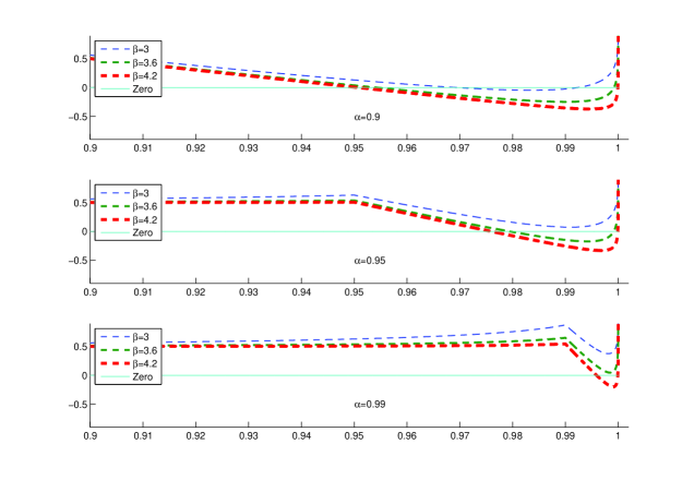
Figure 1: The function $\Psi$ for $\rho=0.5$ and different $\beta$ and $\alpha$.

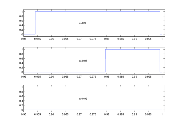
Figure 2: The marginal indemnification function $k^{*}$, for parameters $\beta=3.6$ and $\rho=0.5$.

Example 2.

Let us consider that the ceding company uses $\mathrm{VaR}_{\alpha}$ and the reinsurance company $\mathrm{VaR}_{\beta}$, when $\alpha<\beta$.

$$\Psi(t)=\left\{\begin{array}[]{lll}\rho&F_{X_{0}}(t)<\alpha\\ \rho+1&\alpha\leq F_{X_{0}}(t)<\beta\\ 0&F_{X_{0}}(t)\geq\beta\end{array}\right..$$

This shows that $f(x)=0$, and therefore, the ceding company should not transfer any part of her risk to the reinsurance company. In the opposite direction if $\alpha>\beta$, the same is true for the reinsurance company, that means the reinsurance company has to accept the whole risk.

References

- Acerbi (2002) Acerbi, C. (2002). Spectral measures of risk: A coherent representation of subjective risk aversion. Journal of Banking & Finance 26(7), 1505–1518.
- Arrow (1963) Arrow, K. J. (1963, December). Uncertainty and the welfare economics of medical care. The American Economic Review LIII(5).
- Balbás et al. (2009) Balbás, A., J. Garrido, and S. Mayoral (2009). Properties of distortion risk measures. Methodology and Computing in Applied Probability 11(3), 385–399.
- Bernard and Tian (2009) Bernard, C. and W. Tian (2009). Optimal reinsurance arrangements under tail risk measures. Journal of Risk and Insurance 76(3), 709–725.
- Borch (1960) Borch, K. (1960). An attempt to determine the optimum amount of stop loss reinsurance. Transactions of the 16th International Congress of Actuaries I(3), 597–610.
- Cai and Tan (2007) Cai, J. and K. S. Tan (2007). Optimal retention for a stop-loss reinsurance under the VaR and CTE risk measures. Astin Bull. 37(1), 93–112.
- Cai et al. (2008) Cai, J., K. S. Tan, C. Weng, and Y. Zhang (2008). Optimal reinsurance under VaR and CTE risk measures. Insurance Math. Econom. 43(1), 185–196.
- Cheung et al. (2014) Cheung, K., K. Sung, S. Yam, and S. Yung (2014). Optimal reinsurance under general law-invariant risk measures. Scandinavian Actuarial Journal 2014(1), 72–91.
- Cheung (2010) Cheung, K. C. (2010). Optimal reinsurance revisited—a geometric approach. Astin Bull. 40(1), 221–239.
- Chi and Tan (2013) Chi, Y. and K. S. Tan (2013). Optimal reinsurance with general premium principles. Insurance: Mathematics and Economics 52(2), 180 – 189.
- Cont et al. (2010) Cont, R., R. Deguest, and G. Scandolo (2010). Robustness and sensitivity analysis of risk measurement procedures. Quantitative Finance 10(6), 593–606.
- Heimer (1989) Heimer, C. A. (1989). Reactive risk and rational action: Managing moral hazard in insurance contracts, Volume 6. Univ of California Press.
- Kaluszka (2001) Kaluszka, M. (2001). Optimal reinsurance under mean-variance premium principles. Insurance Math. Econom. 28(1), 61–67.
- Kusuoka (2001) Kusuoka, S. (2001). On law invariant coherent risk measures. In Advances in mathematical economics, Vol. 3, Volume 3 of Adv. Math. Econ., pp. 83–95. Tokyo: Springer.
- Okolewski and Kaluszka (2008) Okolewski, A. and M. Kaluszka (2008). Bounds for expectations of concomitants. Statist. Papers 49(4), 603–618.
- Sereda et al. (2010) Sereda, E., E. Bronshtein, S. Rachev, F. Fabozzi, W. Sun, and S. Stoyanov (2010). Distortion risk measures in portfolio optimization. In J. Guerard, JohnB. (Ed.), Handbook of Portfolio Construction, pp. 649–673. Springer US.
- Wang (1995) Wang, S. (1995). Insurance pricing and increased limits ratemaking by proportional hazards transforms. Insurance Math. Econom. 17(1), 43–54.
- Wang et al. (1997) Wang, S. S., V. R. Young, and H. H. Panjer (1997). Axiomatic characterization of insurance prices. Insurance Math. Econom. 21(2), 173–183.
- Wu and Zhou (2006) Wu, X. and X. Zhou (2006). A new characterization of distortion premiums via countable additivity for comonotonic risks. Insurance: Mathematics and Economics 38(2), 324 – 334.
- Young (1999) Young, V. R. (1999). Optimal insurance under Wang’s premium principle. Insurance Math. Econom. 25(2), 109–122.