Enforcing local non-zero constraints in PDEs and applications to hybrid imaging problems

Abstract.

We study the boundary control of solutions of the Helmholtz and Maxwell equations to enforce local non-zero constraints. These constraints may represent the local absence of nodal or critical points, or that certain functionals depending on the solutions of the PDE do not vanish locally inside the domain. Suitable boundary conditions are classically determined by using complex geometric optics solutions. This work focuses on an alternative approach to this issue based on the use of multiple frequencies. Simple boundary conditions and a finite number of frequencies are explicitly constructed independently of the coefficients of the PDE so that the corresponding solutions satisfy the required constraints. This theory finds applications in several hybrid imaging modalities: some examples are discussed.

1. Introduction

The boundary control of the partial differential equation

(1) $$\left\{\begin{array}[]{l}-{\rm div}(a\,\nabla u_{\omega}^{i})-(\omega^{2}\varepsilon+\mathbf{i}\omega\sigma)u_{\omega}^{i}=0\qquad\text{in $\Omega$,}\\ u_{\omega}^{i}=\varphi_{i}\qquad\text{on $\partial\Omega$,}\end{array}\right.$$

to enforce local non-zero constraints is the main topic of this work, where $\Omega\subseteq\mathbb{R}^{d}$ is a smooth bounded domain, $a\in L^{\infty}(\Omega;\mathbb{R}^{d\times d})$ is a uniformly elliptic symmetric tensor and $\varepsilon,\sigma\in L^{\infty}(\Omega;\mathbb{R})$ satisfy $\varepsilon>0$ and $\sigma\geq 0$. More precisely, we want to find suitable $\varphi_{i}$’s such that the corresponding solutions to (1) satisfy certain non-zero constraints in $\Omega$. For example, we may look for $d+1$ boundary conditions $\varphi_{1},\dots,\varphi_{d+1}$ such that, at least locally

(2) $$\left|u_{\omega}^{1}\right|\geq C,\;\;\left|\det\begin{bmatrix}\nabla u_{\omega}^{2}&\cdots&\nabla u_{\omega}^{d+1}\end{bmatrix}\right|\geq C,\;\;\bigl{|}\det\begin{bmatrix}u_{\omega}^{1}&\cdots&u_{\omega}^{d+1}\\ \nabla u_{\omega}^{1}&\cdots&\nabla u_{\omega}^{d+1}\end{bmatrix}\bigr{|}\geq C$$

for some $C>0$ or, more generally, for $b$ boundary values $\varphi_{1},\dots,\varphi_{b}$ such that the corresponding solutions verify $r$ conditions given by

(3) $$\bigl{|}\zeta^{j}\bigl{(}u_{\omega}^{1},\dots,u_{\omega}^{b}\bigr{)}\bigr{|}\geq C,\qquad j=1,\dots,r,$$

where the maps $\zeta^{j}$ depend on $u_{\omega}^{i}$ and their derivatives. Determinant constraints are very common in elasticity theory. As discussed below, our motivation comes from several hybrid imaging techniques [18].

The problem of constructing such boundary conditions is usually set for a fixed frequency $\omega>0$. The classical way to tackle this problem is by means of the so called complex geometric optics solutions. Introduced by Sylvester and Uhlmann [44], CGO solutions are particular highly oscillatory solutions of the Helmholtz equation (1) in $\mathbb{R}^{d}$ such that for $t\gg 1$ ($a=1$, $d=2$)

$$u^{(t)}(x)\approx e^{tx_{1}}\left(\cos(tx_{2})+\mathbf{i}\sin(tx_{2})\right)\quad\text{in }C^{1}(\overline{\Omega};\mathbb{C}),$$

and can be used to determine suitable illuminations by using the estimates proved by Bal and Uhlmann [22] (see also [19, 18, 15]). For example, setting $\varphi_{1}\approx u_{|\partial\Omega}^{(t)}$, $\varphi_{2}\approx\Re u_{|\partial\Omega}^{(t)}$ and $\varphi_{3}\approx\Im u_{|\partial\Omega}^{(t)}$ gives an open set of boundary conditions whose solutions satisfy the first two constraints of (2). Thus, CGO solutions represent a very important theoretical tool, but have several drawbacks. First, the suitable $\varphi_{i}$’s can only be constructed when the parameters are smooth. Second, since $t\gg 1$, the exponential decay in the first variable gives small lower bounds $C$ and the high oscillations make this approach hardly implementable. Further, the construction depends on the coefficients $a$, $\varepsilon$ and $\sigma$, that are usually unknown in inverse problems. Another construction method uses the Runge approximation, which ensures that locally the solutions behave as in the constant coefficient case [23].

In [1], where the case $\sigma=0$ and the constraints in (2) were considered, we proposed an alternative approach to this issue based on the use of multiple frequencies in a fixed admissible range $\mathcal{A}=[K_{\text{min}},K_{\text{max}}]\subseteq\mathbb{R}_{+}$. The technique relies upon the assumption that the $\varphi_{i}$’s are chosen in such a way that the required constraints are satisfied in the case $\omega=0$, i.e. for the conductivity equation

$$\left\{\begin{array}[]{l}-{\rm div}(a\,\nabla u_{0}^{i})=0\qquad\text{in $\Omega$,}\\ u_{0}^{i}=\varphi_{i}\qquad\text{on $\partial\Omega$,}\end{array}\right.$$

for which the maximum principle and results on the absence of critical points [12, 20] usually make the problem much easier. Under this assumption, there exist a finite $K\subseteq\mathcal{A}$ and an open cover $\Omega=\cup_{\omega\in K}\Omega_{\omega}$ such that the constraints are satisfied in each $\Omega_{\omega}$ for $u_{\omega}^{i}$. The proof is based on the regularity theory and on the holomorphicity of the map $\omega\mapsto u_{\omega}^{i}$.

The main novelty of this paper lies in the fully constructive proof. The set $K$ is constructed explicitly as a uniform sampling of the admissible range $\mathcal{A}$ and depends only on the a priori data. Similarly, the constant $C$ in (3) is estimated a priori and depend on the coefficients only through the a priori bounds. This improvement has been achieved by using a quantitative version of the unique continuation theorem for holomorphic functions proved by Momm [37] and a thorough analysis of (1). We consider here the case $\sigma\geq 0$ and the general constraints (3).

It is natural to study this issue for the full Maxwell’s equations, for which the Helmholtz equation often acts as an approximation in the context of hybrid imaging. Maxwell’s equations read

(4) $$\left\{\begin{array}[]{l}{\rm curl}E_{\omega}^{i}=\mathbf{i}\omega\mu H_{\omega}^{i}\qquad\mbox{ in }\Omega,\\ {\rm curl}H_{\omega}^{i}=-\mathbf{i}(\omega\varepsilon+\mathbf{i}\sigma)E_{\omega}^{i}\qquad\mbox{ in }\Omega,\\ E_{\omega}^{i}\times\nu=\varphi_{i}\times\nu\mbox{ on }\partial\Omega.\end{array}\right.$$

As before, we look for illuminations $\varphi_{i}$ and frequencies $\omega$ such that the corresponding solutions verify $r$ conditions given by

(5) $$\bigl{|}\zeta^{j}\bigl{(}(E_{\omega}^{1},H_{\omega}^{1}),\dots,(E_{\omega}^{b},H_{\omega}^{b})\bigr{)}\bigr{|}\geq C>0,\qquad j=1,\dots,r.$$

An example of such conditions is given by $\bigl{|}\det\begin{bmatrix}E_{\omega}^{1}&E_{\omega}^{2}&E_{\omega}^{3}\end{bmatrix}\bigr{|}\geq C$. CGO solutions for Maxwell’s equations have been studied by Colton and P iv rinta [30]. As before, they can be used to obtain suitable solutions [29], but have the drawbacks discussed before. In [4], the multi frequency approach was generalised to (4). The contribution of this paper is in the quantitative estimates for the number of needed frequencies and for the constant $C$ in (5), both determined a priori.

This approach has been recently successfully adapted to the conductivity equation with complex coefficients in [16] and to the Helmholtz equation with Robin boundary conditions in [5].

This theory finds applications in several hybrid imaging inverse problems, where the unknown parameters have to be reconstructed from internal data [34, 18, 6, 9]. Many hybrid problems are governed by the Helmholtz equation (1), e.g. microwave imaging by ultrasound deformation [46, 14], quantitative thermo-acoustic [21, 15], transient elastography and magnetic resonance elastography [23]. The internal measurements are always linear or quadratic functionals of $u_{\omega}^{\varphi}$ and of $\nabla u_{\omega}^{\varphi}$. For example, in microwave imaging by ultrasound deformation, that is modelled by (1) with a scalar-valued $a$ and $\sigma=0$, the internal measurements have the form

$$a(x)\left|\nabla u_{\omega}^{\varphi}\right|^{2}(x),\qquad\varepsilon(x)\left|u_{\omega}^{\varphi}\right|(x)^{2},\qquad x\in\Omega,$$

and in thermo-acoustic, modelled by (1) with $a=\varepsilon=1$ and $\sigma>0$, we measure

$$\sigma(x)\left|u_{\omega}^{\varphi}\right|(x)^{2},\qquad x\in\Omega.$$

In order for these measurements to be meaningful at every $x\in\Omega$, they need to be non-zero: otherwise, we would measure only noise. Moreover, we shall see that conditions like (2) or, more generally, (3) for some map $\zeta$, are necessary to reconstruct the unknown parameters $a$, $\varepsilon$ and/or $\sigma$ or to obtain good stability estimates [46, 36, 23]. Thus, being able to determine suitable illuminations independently of the unknown parameters is fundamental, and these can be given by the multi-frequency approach discussed in this paper. It should be mentioned that stability of H lder type has been proved by Alessandrini in the context of microwave imaging with ultrasounds with $a=1$ without requiring any non-zero constraint [11].

Similarly, several problems are modelled by the Maxwell’s equations (4) [32, 24, 29], and the inversion usually requires the availability of solutions satisfying certain non-zero constraints inside the domain, given by (5), for some maps $\zeta^{j}$ depending on the particular problem under consideration. As above, the multi-frequency approach discussed in this work can be applied to all these situations.

It is worth mentioning that the underlying physical principle was employed by Renzhiglova et al. in an experimental study on magneto-acousto-eletrical tomography, where dual-frequency ultrasounds were used to obtain non-zero internal data [40].

This paper is structured as follows. The main results are stated and commented in Section 2, and their proofs are detailed in Section 3. Several applications to hybrid imaging problems are described in Section 4. Some relevant open problems are discussed in Section 5. Finally, some basic tools are presented in Appendix A.

2. Main results

2.1. The Helmholtz equation

Given a smooth bounded domain $\Omega\subseteq\mathbb{R}^{d}$, $d=2,3$, we consider the Dirichlet boundary value problem

(6) $$\left\{\begin{array}[]{l}-{\rm div}(a\,\nabla u_{\omega}^{i})-(\omega^{2}\varepsilon+\mathbf{i}\omega\sigma)\,u_{\omega}^{i}=0\qquad\text{in $\Omega$,}\\ u_{\omega}^{i}=\varphi_{i}\qquad\text{on $\partial\Omega$.}\end{array}\right.$$

We assume that $a\in L^{\infty}(\Omega;\mathbb{R}^{d\times d})$ and $\varepsilon\in L^{\infty}(\Omega;\mathbb{R})$ and satisfy

(7a) $$a=a^{T},\qquad\Lambda^{-1}\left|\xi\right|^{2}\leq\xi\cdot a\xi\leq\Lambda\left|\xi\right|^{2},\qquad\xi\in\mathbb{R}^{d},$$

(7b) $$\Lambda^{-1}\leq\varepsilon\leq\Lambda\;\text{ almost everywhere}$$

for some $\Lambda>0$ and that $\sigma\in L^{\infty}(\Omega;\mathbb{R})$ and satisfies either

(8) $$\sigma=0,\text{ or}$$

(9) $$\Lambda^{-1}\leq\sigma\leq\Lambda\;\text{ almost everywhere.}$$

In electromagnetics, $\varepsilon$ is the electric permittivity, $\sigma$ is the electric conductivity and $a$ is the inverse of the magnetic permeability. Take $\kappa\in\mathbb{N}$ and $\alpha\in(0,1)$. Suppose $\varphi_{i}\in C^{\kappa,\alpha}(\overline{\Omega};\mathbb{C})$ and

(10) $$a\in C^{\kappa-1,\alpha}(\overline{\Omega};\mathbb{R}^{d\times d}),\quad\varepsilon,\sigma\in W^{\kappa-1,\infty}(\Omega;\mathbb{R})\quad\text{if $\kappa\geq 1$.}$$

Let $\mathcal{A}=[K_{min},K_{max}]\subseteq B(0,M)$ represent the frequencies we have access to, for some $0<K_{min}<K_{max}\leq M$. By standard elliptic theory (Proposition 7), problem (6) is well-posed for every $\omega\in D$, where

(11) $$D=\begin{cases}\mathbb{C}\setminus\sqrt{\Sigma}&\text{if \eqref{eq:sigma equal 0-multi} holds,}\\ \{\omega\in\mathbb{C}:\left|\Im\omega\right|<\eta\}&\text{if \eqref{eq:sigma bounds below-multi} holds.}\end{cases}$$

Here $\Sigma=\{\lambda_{l}:l\in\mathbb{N}^{*}\}$ is the set of the Dirichlet eigenvalues of problem (6) ($\sqrt{\Sigma}=\{\omega\in\mathbb{C}:\omega^{2}\in\Sigma\}$), and $\eta>0$ depends only on $\Omega$ and $\Lambda$. Figure 1 represents the domain $D$ and the admissible set of frequencies $\mathcal{A}$. Note that $u_{\omega}^{i}\in C^{\kappa}(\overline{\Omega};\mathbb{C})$ by elliptic regularity theory (Proposition 8).

Definition 1.

Given a finite set $K\subseteq\mathcal{A}$ and $\varphi_{1},\dots,\varphi_{b}\in C^{\kappa,\alpha}(\overline{\Omega};\mathbb{C})$, we say that $K\times\{\varphi_{1},\dots,\varphi_{b}\}$ is a set of measurements.

We shall study a particular class of sets of measurements, namely those whose corresponding solutions $u_{\omega}^{i}$ ($i=1,\dots,b$) to (6) and their derivatives up to the $\kappa$-th order satisfy $r$ constraints in $\Omega$. These are described by a map $\zeta$. For $b,r\in\mathbb{N}^{*}$ let

(12a) $$\zeta=(\zeta^{1},\dots,\zeta^{r})\colon C^{\kappa}(\overline{\Omega};\mathbb{C}){}^{b}\longrightarrow C(\overline{\Omega};\mathbb{C})^{r}\;\text{ be holomorphic, such that}$$

(12b) $$\bigl{\|}\zeta(u^{1},\dots,u^{b})\bigr{\|}_{C(\overline{\Omega};\mathbb{C})^{r}}\leq c_{\zeta}(1+\bigl{\|}(u^{1},\dots,u^{b})\bigr{\|}_{C^{\kappa}(\overline{\Omega};\mathbb{C}){}^{b}}^{s})\text{ and}$$

(12c) $$\bigl{\|}D\zeta_{(u^{1},\dots,u^{b})}\bigr{\|}_{\mathcal{B}(C^{\kappa}(\overline{\Omega};\mathbb{C}){}^{b},C(\overline{\Omega};\mathbb{C})^{r})}\leq c_{\zeta}(1+\bigl{\|}(u^{1},\dots,u^{b})\bigr{\|}_{C^{\kappa}(\overline{\Omega};\mathbb{C}){}^{b}}^{s})$$

for some $c_{\zeta}>0$ and $s\in\mathbb{N}^{*}$. (For the definition of holomorphic function, see $\S$ 3.1.) We shall use the notation $C_{\zeta}=(c_{\zeta},s,r,\kappa,\alpha)$.

Example 1.

We consider here the constraints given in (2). Take $b=d+1$, $r=3$ and $\kappa=1$ and let $\zeta_{\det}\colon C^{1}(\overline{\Omega};\mathbb{C}){}^{d+1}\longrightarrow C(\overline{\Omega};\mathbb{C})^{3}$ be defined by

$$\zeta_{\det}^{1}(u^{1},\dots,u^{d+1})=u^{1},$$

$$\zeta_{\det}^{2}(u^{1},\dots,u^{d+1})=\det\begin{bmatrix}\nabla u^{2}&\cdots&\nabla u^{d+1}\end{bmatrix},$$

$$\zeta_{\det}^{3}(u^{1},\dots,u^{d+1})=\det\begin{bmatrix}u^{1}&\cdots&u^{d+1}\\ \nabla u^{1}&\cdots&\nabla u^{d+1}\end{bmatrix}.$$

The map $\zeta_{\det}$ is holomorphic (Lemma 1). Simple calculations show that (12b) holds true with $s_{b}=d+1$ and (12c) with $s_{c}=d$, and so we can set $s=d+1$.

We introduce the particular class of sets of measurements we are interested in.

Definition 2.

Take $\Omega^{\prime}\subseteq\Omega$. Let $b,r\in\mathbb{N}^{*}$ be two positive integers, $C>0$ and let $\zeta$ be as in (12). A set of measurements $K\times\{\varphi_{1},\dots,\varphi_{b}\}$ is $(\zeta,C)$-complete in $\Omega^{\prime}$ if there exists an open cover of $\Omega^{\prime}$

$$\Omega^{\prime}=\bigcup_{\omega\in K\cap D}\Omega^{\prime}_{\omega},$$

such that for any $\omega\in K\cap D$

(13) $$\bigl{|}\zeta^{j}\bigl{(}u_{\omega}^{1},\dots,u_{\omega}^{b}\bigr{)}(x)\bigr{|}\geq C,\qquad j=1,\dots,r,\;x\in\Omega^{\prime}_{\omega}.$$

Namely, a $(\zeta,C)$-complete set gives a cover of $\Omega^{\prime}$ into $\#(K\cap D)$ subdomains, such that the constraints given in (13) are satisfied in each subdomain for different frequencies.

We now describe how to choose the frequencies in the admissible set $\mathcal{A}$. Let $K^{(n)}$ be the uniform partition of $\mathcal{A}$ into $n-1$ intervals so that $\#K^{(n)}=n$, namely

(14) $$K^{(n)}=\{\omega_{1}^{(n)},\dots,\omega_{n}^{(n)}\},\qquad\omega_{i}^{(n)}=K_{min}+\frac{(i-1)}{(n-1)}(K_{max}-K_{min}).$$

Set $\left|\mathcal{A}\right|=K_{max}-K_{min}$. The main result of this paper regarding the Helmholtz equation reads as follows.

Theorem 1.

Assume that (7), (10) and either (8) or (9) hold. Let $\zeta$ be as in (12) and assume that there exist $\varphi_{1},\dots,\varphi_{b}\in C^{\kappa,\alpha}(\overline{\Omega};\mathbb{C})$ and $C_{0}>0$ such that

(15) $$\bigl{|}\zeta^{j}\bigl{(}u_{0}^{1},\dots,u_{0}^{b}\bigr{)}(x)\bigr{|}\geq C_{0},\quad j=1,\dots,r,\;x\in\Omega^{\prime}.$$

Then there exist $C>0$ and $n\in\mathbb{N}$ depending on $\Omega$, $\Lambda$, $\left|\mathcal{A}\right|$, $M$, $C_{\zeta}$, $\left\|a\right\|_{C^{\kappa-1,\alpha}(\overline{\Omega};\mathbb{R}^{d\times d})}$, $\left\|(\varepsilon,\sigma)\right\|_{W^{\kappa-1,\infty}(\Omega;\mathbb{R})^{2}}$, $\left\|\varphi_{i}\right\|_{C^{\kappa,\alpha}(\overline{\Omega};\mathbb{C})}$ and $C_{0}$ such that

$$K^{(n)}\times\{\varphi_{1},\dots,\varphi_{b}\}$$

is a $(\zeta,C)$-complete set of measurements in $\Omega^{\prime}$.

We now discuss assumption (15), the dependence of $C$ on $\left|\mathcal{A}\right|$ and $M$ and the regularity assumption on the coefficients.

Remark 1.

This result allows an a priori construction of $(\zeta,C)$-complete sets, since $C$ and $n$ depend only on a priori data, provided that $\varphi_{1},\dots,\varphi_{b}$ are chosen in such a way that (15) holds true. It is in general easier to satisfy (15) than (13), as $\omega=0$ makes problem (6) simpler. More precisely, there exist many results regarding the conductivity equation [12, 28, 47, 20, 19] (see also the proof of Corollary 1). It is worth noting that, especially in 3D, satisfying (15) may still be highly non trivial, and the strategy used for the case $\omega=0$ may be applicable for higher frequencies as well.

Note that (6) with $\omega=0$ does not depend on $\varepsilon$ and $\sigma$, so that the construction of $\varphi_{1},\dots,\varphi_{b}$ is always independent of $\varepsilon$ and $\sigma$ but may depend on $a$.

There exist occulting illuminations, i.e. boundary conditions for which a finite number of frequencies are not sufficient, and so assumption (15) cannot be completely removed [1]. Yet, this assumption can be weakened (see Remark 6).

Remark 2.

The proof of this result is based on Lemma 3. Thus, the constant $C$ goes to zero as $\left|\mathcal{A}\right|\to 0$, $M\to\infty$ or $C_{0}\to 0$ (see Remark 9 for the precise dependence). In particular, this approach gives good estimates for frequencies in a moderate regime (e.g. with microwaves), but these estimates get worse for very high frequencies. This should be taken into account in the presence of noisy measurements.

Remark 3.

The regularity of the coefficients required for this approach is lower than the regularity required if CGO solutions are used. Indeed, consider for simplicity the constraints given by the map $\zeta_{\det}$ and suppose $a=1$ and $\sigma=0$. The CGO approach requires $\varepsilon\in C^{1}$ [22], while with this method we only assume $\varepsilon\in L^{\infty}$.

Similarly, the approach based on the Runge approximation property requires $a$ to be Lipschitz continuous, in addition to (10) [23]. Therefore, higher regularity assumptions are needed in the cases when $\kappa=0,1$.

We now apply Theorem 1 to the case $\zeta=\zeta_{\det}$. The construction of $(\zeta_{\det},C)$-complete sets of measurements depends on the dimension, since the validity of (15) for $\zeta_{\det}^{2}$ and $\zeta_{\det}^{3}$ depends on the dimension.

Corollary 1.

Assume that (7), (10) and either (8) or (9) hold for $\kappa=1$.

If $d=2$, $\Omega$ is convex and $\Omega^{\prime}\Subset\Omega$ then there exist $C>0$ and $n\in\mathbb{N}$ depending on $\Omega$, $\Omega^{\prime}$, $\Lambda$, $\alpha$, $\left|\mathcal{A}\right|$, $M$ and $\left\|a\right\|_{C^{0,\alpha}(\overline{\Omega};\mathbb{R}^{2\times 2})}$ such that

$$K^{(n)}\times\{1,x_{1},x_{2}\}$$

is a $(\zeta_{\det},C)$-complete set of measurements in $\Omega^{\prime}$.

If $d=3$ and $\hat{a}\in\mathbb{R}^{3\times 3}$ is a constant tensor satisfying (7a) then there exist $\delta,C>0$ and $n\in\mathbb{N}$ depending on $\Omega$, $\Lambda$, $\alpha$, $\left|\mathcal{A}\right|$, $M$ and $\left\|a\right\|_{C^{0,\alpha}(\overline{\Omega};\mathbb{R}^{3\times 3})}$ such that if $\left\|a-\hat{a}\right\|_{C^{0,\alpha}(\overline{\Omega};\mathbb{R}^{3\times 3})}\leq\delta$ then

$$K^{(n)}\times\{1,x_{1},x_{2},x_{3}\}$$

is a $(\zeta_{\det},C)$-complete set of measurements in $\Omega$.

Remark 4.

In 2D, it is possible to consider non-convex domains, provided that the boundary conditions are chosen in accordance to Lemma 10 [25, 1].

Remark 5.

In order to satisfy the constraints corresponding to $\zeta_{\det}^{1}$, by the strong maximum principle it is enough to choose $\varphi_{1}\geq C_{0}>0$. As far as (15) for $\zeta_{\det}^{3}$ is concerned, it is sufficient to set $\varphi_{2}=x_{1}\varphi_{1}$ and $\varphi_{3}=x_{2}\varphi_{1}$ [1].

Remark 6.

The difference between the two and three dimensional case is due to the presence of critical points in the case $\omega=0$ in 3D [26, 17, 27]. In order to satisfy (15) in 3D we assume that $a$ is close to a constant matrix. This assumption can be removed in some situations by using a different approach in $\omega=0$ [20] or by choosing generic boundary conditions [3]: in these cases, the a priori estimates on $C$ and $n$ are lost. If the constraints do not involve gradient fields, e.g. $\zeta=\zeta_{\det}^{1}$, then there is no need for this assumption.

2.2. Maxwell’s equations

Given a smooth bounded domain $\Omega\subseteq\mathbb{R}^{3}$ with a simply connected boundary $\partial\Omega$, in this subsection we consider Maxwell’s equations

(16) $$\left\{\begin{array}[]{l}{\rm curl}E_{\omega}^{i}=\mathbf{i}\omega\mu H_{\omega}^{i}\qquad\text{in $\Omega$,}\\ {\rm curl}H_{\omega}^{i}=-\mathbf{i}(\omega\varepsilon+\mathbf{i}\sigma)E_{\omega}^{i}\qquad\text{in $\Omega$,}\\ E_{\omega}^{i}\times\nu=\varphi_{i}\times\nu\qquad\text{on $\partial\Omega$,}\end{array}\right.$$

with $\mu,\varepsilon,\sigma\in L^{\infty}(\Omega;\mathbb{R}^{3\times 3})$ and $\varphi_{i}$ satisfying

(17a) $$\Lambda^{-1}\left|\xi\right|^{2}\leq\xi\cdot\mu\xi,\quad\Lambda^{-1}\left|\xi\right|^{2}\leq\xi\cdot\varepsilon\xi,\quad\Lambda^{-1}\left|\xi\right|^{2}\leq\xi\cdot\sigma\xi,\qquad\xi\in\mathbb{R}^{3},$$

(17b) $$\left\|(\mu,\varepsilon,\sigma)\right\|_{L^{\infty}(\Omega;\mathbb{R}^{3\times 3})^{3}}\leq\Lambda,\;\mu=\mu^{T},\;\varepsilon=\varepsilon^{T},\;\sigma=\sigma^{T},\;\mu,\varepsilon,\sigma\in W^{\kappa+1,p}(\Omega),$$

(17c) $${\rm curl}\varphi_{i}\cdot\nu=0\text{ on $\partial\Omega$}\text{ and }\varphi_{i}\in W^{\kappa+1,p}(\Omega;\mathbb{C}^{3})$$

for some $\Lambda>0$, $\kappa\in\mathbb{N}$ and $p>3$. The electromagnetic fields $E_{\omega}^{i}$ and $H_{\omega}^{i}$ satisfy

$$E_{\omega}^{i}\in H({\rm curl},\Omega):=\{u\in L^{2}(\Omega;\mathbb{C}^{3}):{\rm curl}u\in L^{2}(\Omega;\mathbb{C}^{3})\},$$

$$H_{\omega}^{i}\in H^{\mu}({\rm curl},\Omega):=\{v\in H({\rm curl},\Omega):{\rm div}(\mu v)=0\text{ in $\Omega$, }\mu v\cdot\nu=0\text{ on }\partial\Omega\}.$$

The matrix $\varepsilon$ represents the electric permittivity, $\sigma$ is the electric conductivity and $\mu$ stands for the magnetic permeability. Note that $(E_{\omega}^{i},H_{\omega}^{i})\in C^{\kappa}(\overline{\Omega};\mathbb{C}^{6})$ by Proposition 10.

Definition 3.

Given a finite set $K\subseteq\mathcal{A}$ and $\varphi_{1},\dots,\varphi_{b}\in W^{\kappa+1,p}(\Omega;\mathbb{C}^{3})$ satisfying (17c), we say that $K\times\{\varphi_{1},\dots,\varphi_{b}\}$ is a set of measurements.

As before, we are interested in a particular class of sets of measurements, namely those whose corresponding solutions $(E_{\omega}^{i},H_{\omega}^{i})$ to (16) and their derivatives up to the $\kappa$-th order satisfy $r$ non-zero constraints inside the domain. These are described by a map $\zeta$, which we now introduce. For $b,r\in\mathbb{N}^{*}$ let

(18a) $$\zeta=(\zeta^{1},\dots,\zeta^{r})\colon C^{\kappa}(\overline{\Omega};\mathbb{C}^{6}){}^{b}\longrightarrow C(\overline{\Omega};\mathbb{C})^{r}\;\text{ be holomorphic, such that}$$

(18b) $$\bigl{\|}\zeta((u^{i},v^{i})_{i})\bigr{\|}_{C(\overline{\Omega};\mathbb{C})^{r}}\leq c_{\zeta}(1+\bigl{\|}((u^{i},v^{i})_{i})\bigr{\|}_{C^{\kappa}(\overline{\Omega};\mathbb{C}^{6}){}^{b}}^{s}),$$

(18c) $$\bigl{\|}D\zeta_{((u^{i},v^{i})_{i})}\bigr{\|}_{\mathcal{B}(C^{\kappa}(\overline{\Omega};\mathbb{C}^{6}){}^{b},C(\overline{\Omega};\mathbb{C})^{r})}\!\leq\!c_{\zeta}(1+\bigl{\|}((u^{i},v^{i})_{i})\bigr{\|}_{C^{\kappa}(\overline{\Omega};\mathbb{C}^{6}){}^{b}}^{s})$$

for some $c_{\zeta}>0$ and $s\in\mathbb{N}^{*}$. We shall use the notation $C_{\zeta}=(c_{\zeta},s,r,\kappa,p)$.

We now consider one example of map $\zeta$. For other examples, see [4].

Example 2.

Take $b=3$, $r=1$, $\kappa=0$ and let $\zeta_{\det}^{M}$ be defined by

$$\zeta_{\det}^{M}((u_{1},v_{1}),(u_{2},v_{2}),(u_{3},v_{3}))=\det\begin{bmatrix}u_{1}&u_{2}&u_{3}\end{bmatrix},\qquad(u_{i},v_{i})\in C(\overline{\Omega};\mathbb{C}^{6}).$$

The map $\zeta_{\det}^{M}$ is multilinear and bounded, whence holomorphic by Lemma 1. Assumptions (18b) and (18c) are obviously verified. In this case, the condition characterising $(\zeta_{\det}^{M},C)$-complete sets of measurements is $\bigl{|}\det\begin{bmatrix}E_{\omega}^{1}&E_{\omega}^{2}&E_{\omega}^{3}\end{bmatrix}(x)\bigr{|}\geq C$. In other words, this constraints signals the availability, in every point, of three independent electric fields and, in particular, of one non-vanishing electric field.

We now give the precise definition of $(\zeta,C)$-complete sets of measurements for Maxwell’s equations. The only difference with the Helmholtz equation is that here, for simplicity, we require the constraints to hold in the whole domain $\Omega$.

Definition 4.

Let $b,r\in\mathbb{N}^{*}$ be two positive integers, $C>0$ and let $\zeta$ be as in (18). A set of measurements $K\times\{\varphi_{1},\dots,\varphi_{b}\}$ is $(\zeta,C)$-complete if there exists an open cover of $\Omega$, $\Omega=\cup_{\omega\in K}\Omega{}_{\omega}$, such that for any $\omega\in K$

(19) $$\bigl{|}\zeta^{j}\bigl{(}(E_{\omega}^{1},H_{\omega}^{1}),\dots,(E_{\omega}^{b},H_{\omega}^{b})\bigr{)}(x)\bigr{|}\geq C,\qquad j=1,\dots,r,\;x\in\Omega{}_{\omega}.$$

Let $K^{(n)}$ be as in (14). The main result of this subsection reads as follows.

Theorem 2.

Assume that (17) holds. Let $\hat{\sigma}\in W^{\kappa,p}(\Omega;\mathbb{R}^{3\times 3})$ satisfy (17a). Let $\zeta$ be as in (18) and assume that there exist $\varphi_{1},\dots,\varphi_{b}\in W^{\kappa+1,p}(\Omega;\mathbb{C}^{3})$ satisfying (17c) and $C_{0}>0$ such that

(20) $$\bigl{|}\zeta^{j}\bigl{(}(\hat{E}_{0}^{1},\hat{H}_{0}^{1}),\dots,(\hat{E}_{0}^{b},\hat{H}_{0}^{b})\bigr{)}(x)\bigr{|}\geq C_{0},\qquad x\in\Omega,\,j=1,\dots,r,$$

where $(\hat{E}{}_{0}^{i},\hat{H}_{0}^{i})\in H({\rm curl},\Omega)\times H^{\mu}({\rm curl},\Omega)$ is the solution to (16) with $\hat{\sigma}$ in lieu of $\sigma$ and $\omega=0$, namely

(21) $$\left\{\begin{array}[]{l}{\rm curl}\hat{E}{}_{0}^{i}=0\qquad\text{in $\Omega$,}\\ {\rm div}(\hat{\sigma}\hat{E}{}_{0}^{i})=0\qquad\text{in $\Omega$,}\\ \hat{E}{}_{0}^{i}\times\nu=\varphi_{i}\times\nu\qquad\text{on $\partial\Omega$,}\end{array}\right.\qquad\left\{\begin{array}[]{l}{\rm curl}\hat{H}_{0}^{i}=\hat{\sigma}\hat{E}{}_{0}^{i}\qquad\text{in $\Omega$,}\\ {\rm div}(\mu\hat{H}_{0}^{i})=0\qquad\text{in $\Omega$,}\\ \mu\hat{H}_{0}^{i}\cdot\nu=0\qquad\text{on $\partial\Omega$.}\end{array}\right.$$

There exist $\delta,C>0$ and $n\in\mathbb{N}$ depending on $\Omega$, $\Lambda$, $\left|\mathcal{A}\right|$, $M$, $C_{\zeta}$, $\left\|\varphi_{i}\right\|_{W^{\kappa+1,p}(\overline{\Omega};\mathbb{C}^{3})}$, $\left\|(\varepsilon,\sigma,\mu)\right\|_{W^{\kappa+1,p}(\overline{\Omega};\mathbb{R}^{3\times 3})}$ and $C_{0}$ such that if $\left\|\sigma-\hat{\sigma}\right\|_{W^{\kappa+1,p}(\overline{\Omega};\mathbb{R}^{3\times 3})}\leq\delta$ then

$$K^{(n)}\times\{\varphi_{1},\dots,\varphi_{b}\}$$

is a $(\zeta,C)$-complete set of measurements.

We now discuss assumption (20), the dependence of the construction of the illuminations on the electromagnetic parameters and the regularity assumption on the coefficients (see Remarks 1 and 3).

Remark 7.

Suppose that we are in the simpler case $\hat{\sigma}=\sigma$. Note that (21) does not depend on $\varepsilon$, so that the construction of $\varphi_{1},\dots,\varphi_{b}$ is always independent of $\varepsilon$ but may depend on $\sigma$ and $\mu$. However, in the cases where the maps $\zeta^{j}$ involve only the electric field $E$, it depends on $\sigma$, and not on $\varepsilon$ and $\mu$ (see Corollary 2).

A typical application of the theorem is in the case where $\sigma$ is a small perturbation of a known constant tensor $\hat{\sigma}$. Then, the construction of $\varphi_{1},\dots,\varphi_{b}$ is independent of $\sigma$. A similar argument would work if $\mu$ were a small perturbation of a constant tensor $\hat{\mu}$. We have decided to omit it for simplicity, since in the applications we have in mind the maps $\zeta^{j}$ do not depend on the magnetic field $H$.

Remark 8.

The regularity of the coefficients required for this approach is much lower than the regularity required if CGO solutions are used. Indeed, if the constraints depend on the derivatives up to the $\kappa$-th order, with this approach we require the parameters to be in $W^{\kappa+1,p}$, while with CGO we need $W^{\kappa+3,p}$ [29].

In the case where the conditions given by the map $\zeta$ are independent of the magnetic field $H$, Theorem 2 can be rewritten in the following form.

Corollary 2.

Assume that (17) holds. Let $\hat{\sigma}\in W^{\kappa,p}(\Omega;\mathbb{R}^{3\times 3})$ satisfy (17a) and $\zeta$ be as in (18) and independent of $H$. Take $\psi_{1},\dots,\psi_{b}\in W^{\kappa+2,p}(\Omega;\mathbb{C})$. Suppose

(22) $$\bigl{|}\zeta^{j}\bigl{(}\nabla w^{1},\dots,\nabla w^{b}\bigr{)}(x)\bigr{|}\geq C_{0},\qquad x\in\Omega,\,j=1,\dots,r$$

for some $C_{0}>0$, where $w^{i}\in H^{1}(\Omega;\mathbb{C})$ is the solution to

$$\left\{\begin{array}[]{l}{\rm div}(\hat{\sigma}\nabla w^{i})=0\qquad\text{in $\Omega$,}\\ w^{i}=\psi_{i}\qquad\text{on $\partial\Omega$.}\end{array}\right.$$

There exist $\delta,C>0$ and $n\in\mathbb{N}$ depending on $\Omega$, $\Lambda$, $\left|\mathcal{A}\right|$, $M$, $C_{\zeta}$, $\left\|\psi_{i}\right\|_{W^{\kappa+2,p}(\overline{\Omega};\mathbb{C}^{3})}$, $\left\|(\varepsilon,\sigma,\mu)\right\|_{W^{\kappa+1,p}(\overline{\Omega};\mathbb{R}^{3\times 3})}$ and $C_{0}$ such that if $\left\|\sigma-\hat{\sigma}\right\|_{W^{\kappa+1,p}(\overline{\Omega};\mathbb{R}^{3\times 3})}\leq\delta$ then

$$K^{(n)}\times\{\nabla\psi_{1},\dots,\nabla\psi_{b}\}$$

is a $(\zeta,C)$-complete set of measurements.

In other words, if the required constraints do not depend on $H$, then the problem of finding $\zeta$-complete sets is reduced to satisfying the same conditions for the gradients of solutions to the conductivity equation, as with the Helmholtz equation.

3. Non-zero constraints in PDEs

The results stated in Section 2 are proven here. In particular, some preliminary lemmata on holomorphic functions are discussed in $\S$ 3.1, and the proofs of Theorem 1, Corollary 1 and Theorem 2 are given in $\S$ 3.2, $\S$ 3.3 and $\S$ 3.4, respectively.

3.1. Holomorphic functions

Holomorphic functions in a Banach space setting were studied in [45]. Let $E$ and $E^{\prime}$ be complex Banach spaces, $D\subseteq E$ be an open set and take $f\colon D\to E^{\prime}$. We say that $f$ is holomorphic if it is continuous and if

$$\lim_{\tau\to 0}\frac{f(x_{0}+\tau y)-f(x_{0})}{\tau}$$

exists in $E^{\prime}$ for all $x_{0}\in D$ and $y\in E$. This notion extends the classical notion of holomorphicity for functions of complex variable.

This lemma summarises some of the basic properties of holomorphic functions.

Lemma 1.

Let $E_{1},\dots,E_{r}$, $E$ and $E^{\prime}$ be complex Banach spaces and $D\subseteq E$ be an open set.

1. If $f\colon E_{1}\times\dots\times E_{r}\to E^{\prime}$ is multilinear and bounded then $f$ is holomorphic.

2. If $f\colon D\to E_{1}$ and $g\colon E_{1}\to E^{\prime}$ are holomorphic then $g\circ f\colon D\to E^{\prime}$ is holomorphic.

3. Take $f=(f^{1},\dots f^{r})\colon D\to E_{1}\times\dots\times E_{r}$. Then $f$ is holomorphic if and only if $f^{j}$ is holomorphic for every $j=1,\dots,r$.

The following result is a quantitative version of the unique continuation property for holomorphic functions of one complex variable.

Lemma 2.

Take $C_{0},D>0$, $\theta\in(0,1)$ and $r\in(0,\theta]$. Let $g$ be a holomorphic function in $B(0,1)\subseteq\mathbb{C}$ such that $\left|g(0)\right|\geq C_{0}$ and $\sup_{B(0,1)}\left|g\right|\leq D$. There exists $\omega\in[r,1)$ such that

$$\left|g(\omega)\right|\geq C$$

for some constant $C>0$ depending on $\theta$, $C_{0}$ and $D$ only.

Proof.

Since $[\theta,(1+\theta)/2]\subseteq[r,1)$, it is sufficient to show that there exists $C>0$ depending on $\theta$, $C_{0}$ and $D$ only such that

$$\max_{[\theta,(1+\theta)/2]}\left|g\right|\geq C.$$

By contradiction, suppose that there exists a sequence $(g_{n})_{n}$ of holomorphic functions in $B(0,1)$ such that $\sup_{B(0,1)}\left|g_{n}\right|\leq D$, $\left|g_{n}(0)\right|\geq C_{0}$ and $\max_{[\theta,(1+\theta)/2]}\left|g_{n}\right|\to 0$. Since $\sup_{B(0,1)}\left|g_{n}\right|\leq D$, by standard complex analysis, up to a subsequence $g_{n}\to g_{\infty}$ for some $g_{\infty}$ holomorphic in $B(0,1)$. As $\max_{[\theta,(1+\theta)/2]}\left|g_{n}\right|\to 0$, we obtain $g_{\infty}=0$ on $[\theta,(1+\theta)/2]$, whence $g_{\infty}=0$, which contradicts $\left|g_{\infty}(0)\right|\geq C_{0}$.∎

Remark 9.

Although elementary, the proof of Lemma 2 does not give the dependence of the constant $C$ on the parameters $\theta$, $C_{0}$ and $D$.

By [37] there is a Jordan curve $\Gamma$ in $r<\left|\omega\right|<1$ around the origin such that

$$\log\left|g(\omega)/g(0)\right|\geq-\frac{\tilde{C}}{1-r}\biggl{(}\int_{0}^{1}\left(\frac{\log\sup_{B(0,t)}\left|g/g(0)\right|}{1-t}\right)^{1/2}dt\biggr{)}^{2},\qquad\omega\in\Gamma,$$

for an absolute constant $\tilde{C}>0$. By the Jordan curve theorem there exists $\omega\in(r,1)$ such that

$$\log\left|g(\omega)/g(0)\right|\geq-\frac{\tilde{C}\log(DC_{0}^{-1})}{1-r}.$$

Therefore $\left|g(\omega)\right|\geq\left|g(0)\right|(DC_{0}^{-1})^{-\frac{\tilde{C}}{1-r}}\geq C_{0}(DC_{0}^{-1})^{-\frac{\tilde{C}}{1-r}}\geq C_{0}(DC_{0}^{-1})^{-\frac{\tilde{C}}{1-\theta}}$, whence the constant given in Lemma 2 is $C=C_{0}(DC_{0}^{-1})^{-\frac{\tilde{C}}{1-\theta}}$.

It is possible to generalise the previous result to functions defined in an ellipse. The proof is elementary, but needed to show the precise dependence of $C$ on $R_{1}-r$.

Lemma 3.

Take $0<r<R_{1}\leq M$ and $0<\eta\leq R_{2}$. Let $g$ be a holomorphic function in the ellipse

$$E=\{\omega\in\mathbb{C}:\frac{(\Re\omega)^{2}}{R_{1}^{2}}+\frac{(\Im\omega)^{2}}{R_{2}^{2}}<1\}$$

such that $\left|g(0)\right|\geq C_{0}>0$ and $\sup_{E}\left|g\right|\leq D$. There exists $\omega\in(r,R_{1})$ such that

$$\left|g(\omega)\right|\geq C$$

for some constant $C>0$ depending on $M$, $R_{1}-r$, $\eta$, $C_{0}$ and $D$ only.

Proof.

Without loss of generality, we can always suppose $R_{2}\leq R_{1}$.

Set $\beta:=\sqrt{R_{1}^{2}+R_{2}^{2}}\leq\sqrt{2}M$, $r_{i}=R_{i}/\beta$ and $\tilde{E}:=\{\omega\in\mathbb{C}:\frac{(\Re\omega)^{2}}{r_{1}^{2}}+\frac{(\Im\omega)^{2}}{r_{2}^{2}}<1\}$. The map $\psi_{1}\colon\tilde{E}\to E$, $\omega\mapsto\beta\omega$ is bi-holomorphic and the segment $(r,R_{1})\subseteq E$ is transformed via $\psi_{1}^{-1}$ into $(r/\beta,R_{1}/\beta)\subseteq\tilde{E}$. Consider now a bi-holomorphic transformation $\psi_{2}\colon B(0,1)\to\tilde{E}$. The existence of this map is a consequence of the Riemann mapping theorem, and an explicit formula is given in [38, page 296]. In particular, $\psi_{2}$ can be chosen so that $\psi_{2}(0)=0$ and $\psi_{2}^{-1}((r/\beta,R_{1}/\beta))=(r^{\prime},1)$ for some $r^{\prime}\in(0,1)$. Since $(R_{1}-r)/\beta\geq(R_{1}-r)/(\sqrt{2}M)$ and $1\leq r_{1}/r_{2}=R_{1}/R_{2}\leq M/\eta$ we have $1-r^{\prime}\geq c$ for some $c>0$ depending only on $M$, $R_{1}-r$, $\eta$, $C_{0}$ and $D$, as the ratio $r_{1}/r_{2}$ determines the deformation carried out by $\psi_{2}$. Hence $r^{\prime}\leq\theta$ with $\theta=1-c$.

Consider now the map $g^{\prime}\colon B(0,1)\to\mathbb{C}$ defined by $g^{\prime}=g\circ\psi_{1}\circ\psi_{2}$. We have that $g^{\prime}$ is holomorphic in $B(0,1)$, $\left|g^{\prime}(0)\right|=\left|g(0)\right|\geq C_{0}$ and $\sup_{B(0,1)}\left|g^{\prime}\right|=\sup_{E}\left|g\right|\leq D$. By Lemma 2 applied to $g^{\prime}$ and $r^{\prime}$ we obtain the result. ∎

3.2. The Helmholtz equation

We prove here Theorem 1. For simplicity, we shall say that a positive constant depends on a priori data if it depends on $\Omega$, $\Lambda$, $\left|\mathcal{A}\right|$, $M$, $C_{\zeta}$, $\left\|a\right\|_{C^{\kappa-1,\alpha}(\overline{\Omega};\mathbb{R}^{d\times d})}$, $\left\|(\varepsilon,\sigma)\right\|_{W^{\kappa-1,\infty}(\Omega;\mathbb{R})^{2}}$, $\left\|\varphi_{i}\right\|_{C^{\kappa,\alpha}(\overline{\Omega};\mathbb{C})}$ and $C_{0}$ only. Recall that $D$ is given by (11) and that $\Sigma=\{\lambda_{l}:l\in\mathbb{N}^{*}\}$ denotes the set of the Dirichlet eigenvalues of problem (6). During the proof, we shall often refer to the results given in the Appendix.

We first show that the map $\omega\in D\mapsto u_{\omega}^{i}\in C^{\kappa}$ is holomorphic. This will be one of the basic tools of the proof of Theorem 1.

Proposition 1.

Under the assumptions of Theorem 1, the map

$$D\longrightarrow C^{\kappa}(\overline{\Omega};\mathbb{C}),\quad\omega\longmapsto u_{\omega}^{i}$$

is holomorphic.

Proof.

In view of Propositions 7 and 8, problem (6) is well-posed and $u_{\omega}^{i}\in C^{\kappa}$. If (8) holds, this result has already been proved in [1]. The case where (9) holds can be handled similarly [2]. ∎

Define for every $j=1,\dots,r$

$$\theta^{j}\colon D\to C(\overline{\Omega};\mathbb{C}),\;\omega\mapsto\zeta^{j}\bigl{(}u_{\omega}^{1},\dots,u_{\omega}^{b}\bigr{)}.$$

As a consequence of the previous result, the maps $\theta^{j}$ are holomorphic.

Lemma 4.

Under the hypotheses of Theorem 1, the map $\theta^{j}\colon D\to C(\overline{\Omega};\mathbb{C})$ is holomorphic for all $j$.

Proof.

It follows from Proposition 1, (12a) and Lemma 1, parts 2 and 3. ∎

Figure 1. The domain $D$ and the admissible set $\mathcal{A}$.

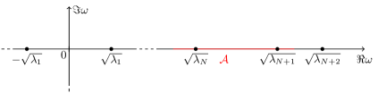
(a) $D=\mathbb{C}\setminus\sqrt{\Sigma}$ if $\eqref{eq:sigma equal 0-multi}$ holds.

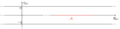
(b) $D=\{\omega\in\mathbb{C}:\left|\Im\omega\right|<\eta\}$ if $\eqref{eq:sigma bounds below-multi}$ holds.

We next study some a priori bounds on $\theta^{j}$ and $\partial_{\omega}\theta^{j}$ (notation of Proposition 7).

Lemma 5.

Assume that the hypotheses of Theorem 1 hold true and take $j=1,\dots,r$ and $\omega\in B(0,M)\cap D$.

1. If (8) holds true then there exists $C>0$ depending on a priori data such that

   1. $\bigl{\|}\theta_{\omega}^{j}\bigr{\|}_{C(\overline{\Omega};\mathbb{C})}\leq C\left[1+\sup_{l\in\mathbb{N}^{*}}\frac{1}{\left|\lambda_{l}-\omega^{2}\right|}\right]^{s}$;

   2. $\bigl{\|}\partial_{\omega}\theta_{\omega}^{j}\bigr{\|}_{C(\overline{\Omega};\mathbb{C})}\leq C\left[1+\sup_{l\in\mathbb{N}^{*}}\frac{1}{\left|\lambda_{l}-\omega^{2}\right|}\right]^{s+2}$.

2. If (9) holds true then there exists $C>0$ depending on a priori data such that

   1. $\bigl{\|}\theta_{\omega}^{j}\bigr{\|}_{C(\overline{\Omega};\mathbb{C})}\leq C$;

   2. $\bigl{\|}\partial_{\omega}\theta_{\omega}^{j}\bigr{\|}_{C(\overline{\Omega};\mathbb{C})}\leq C$.

Proof.

We first prove part 1, namely we take $\sigma=0$. In view of Proposition 7, part 1 and Proposition 8 we have

(23) $$\left\|u_{\omega}^{i}\right\|_{C^{\kappa}(\overline{\Omega};\mathbb{C})}\leq C\left[1+\sup_{l\in\mathbb{N}^{*}}\frac{1}{\left|\lambda_{l}-\omega^{2}\right|}\right],\qquad\omega\in B(0,M)\cap D,$$

whence we obtain part 1a from (12b).

It can be easily seen that $\partial_{\omega}u_{\omega}^{i}$ is the solution to

$$\left\{\begin{array}[]{l}-{\rm div}(a\,\nabla(\partial_{\omega}u_{\omega}^{i}))-\omega^{2}\varepsilon\,\partial_{\omega}u_{\omega}^{i}=2\omega\varepsilon u_{\omega}^{i}\qquad\text{in $\Omega$,}\\ \partial_{\omega}u_{\omega}^{i}=0\qquad\text{on $\partial\Omega$.}\end{array}\right.$$

Arguing as before, from Proposition 7, part 1 and Proposition 8 we obtain

(24) $$\left\|\partial_{\omega}u_{\omega}^{i}\right\|_{C^{\kappa}(\overline{\Omega};\mathbb{C})}\leq C\left[1+\sup_{l\in\mathbb{N}^{*}}\frac{1}{\left|\lambda_{l}-\omega^{2}\right|}\right]^{2}.$$

Since $\partial_{\omega}\theta_{\omega}^{j}=D\zeta_{(u_{\omega}^{1},\dots,u_{\omega}^{b})}^{j}(\partial_{\omega}u_{\omega}^{1},\dots,\partial_{\omega}u_{\omega}^{b})$ we have

$$\begin{split}\bigl{\|}\partial_{\omega}\theta_{\omega}^{j}\bigr{\|}_{C(\overline{\Omega};\mathbb{C})}&=\bigl{\|}D\zeta_{(u_{\omega}^{1},\dots,u_{\omega}^{b})}^{j}(\partial_{\omega}u_{\omega}^{1},\dots,\partial_{\omega}u_{\omega}^{b})\bigr{\|}_{C(\overline{\Omega};\mathbb{C})}\\ &\leq\bigl{\|}D\zeta_{(u_{\omega}^{1},\dots,u_{\omega}^{b})}^{j}\bigr{\|}_{\mathcal{B}(C^{\kappa}(\overline{\Omega};\mathbb{C}){}^{b},C(\overline{\Omega};\mathbb{C}))}\bigl{\|}(\partial_{\omega}u_{\omega}^{1},\dots,\partial_{\omega}u_{\omega}^{b})\bigr{\|}_{C^{\kappa}(\overline{\Omega};\mathbb{C}){}^{b}}\\ &\leq C\left[1+\sup_{l\in\mathbb{N}^{*}}\frac{1}{\left|\lambda_{l}-\omega^{2}\right|}\right]^{s+2},\end{split}$$

where the last inequality follows from (12c), (23) and (24). Part 1b is now proved.

Part 2 can be proved analogously, by using part 2 of Proposition 7 in lieu of part 1. The details are left to the reader. ∎

In the following two lemmata we study the case where (8) holds true, and how to deal with the presence of the eigenvalues (see Figure 2).

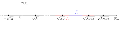
Figure 2. The admissible sets $\mathcal{A}$ and $\tilde{\mathcal{A}}$.

Lemma 6.

Under the hypotheses of Theorem 1, assume that (8) holds true. Then there exist $N\in\mathbb{N}^{*}$, $\delta>0$ and $\beta>0$ depending on $\Omega$, $\Lambda$, $\left|\mathcal{A}\right|$ and $M$ only and a closed interval $\tilde{\mathcal{A}}=[\tilde{K}_{min},\tilde{K}_{max}]\subseteq\mathcal{A}$ such that

$$d(\tilde{\mathcal{A}}^{2},\Sigma)\geq\delta,\qquad\tilde{\mathcal{A}}^{2}\subseteq(\lambda_{l},\lambda_{l+1}),\qquad\bigl{|}\tilde{\mathcal{A}}\bigr{|}\geq\beta$$

for some $l\leq N$, where $\tilde{\mathcal{A}}^{2}=\{\omega^{2}:\omega\in\tilde{\mathcal{A}}\}$.

Proof.

In view of Lemma 9 there exists $N\in\mathbb{N}^{*}$ depending on $\Omega$, $\Lambda$ and $M$ only such that $[0,K_{max}^{2}]\cap\Sigma\subseteq\{\lambda_{1},\dots,\lambda_{N}\}$. In particular, $\#(\mathcal{A}^{2}\cap\Sigma)\leq N$. Therefore there exists $l\leq N$ such that $\left|\mathcal{A}^{2}\cap(\lambda_{l},\lambda_{l+1})\right|\geq\left|\mathcal{A}^{2}\right|(N+1)^{-1}$. Write $\mathcal{A}^{2}\cap(\lambda_{l},\lambda_{l+1})=[p,q]$ and define $\tilde{\mathcal{A}}$ by $\tilde{\mathcal{A}}^{2}=[p+\frac{\left|\mathcal{A}^{2}\right|}{3(N+1)},q-\frac{\left|\mathcal{A}^{2}\right|}{3(N+1)}]$. This concludes the proof, since $\left|\mathcal{A}^{2}\right|$ depends on $\left|\mathcal{A}\right|$ and $N$ only. ∎

Thanks to Lemma 6, by taking a subinterval of the original admissible set $\mathcal{A}$, without loss of generality we can assume that

(25) $$d(\mathcal{A}^{2},\Sigma)\geq\delta,\qquad\mathcal{A}^{2}\subseteq(\lambda_{l},\lambda_{l+1}),\qquad l\leq N$$

for some $\delta>0$ and $N\in\mathbb{N}^{*}$ depending on $\Omega$, $\Lambda$, $\left|\mathcal{A}\right|$ and $M$ only. Moreover, the new size of $\mathcal{A}$ is comparable with the size of the original $\mathcal{A}$ by means of constants depending on $\Omega$, $\Lambda$, $\left|\mathcal{A}\right|$ and $M$ only.

The main idea is to apply Lemma 3 to the maps $\omega\mapsto\theta_{\omega}^{j}(x)$ and use the fact that in $\omega=0$ they are non-zero. However, in the case where (8) holds true we first need to remove the singularities in the poles $\pm\sqrt{\lambda_{1}},\dots,\pm\sqrt{\lambda_{N}}$.

Lemma 7.

Under the hypotheses of Theorem 1, if (8) and (25) hold true then for any $x\in\Omega$ the function

(26) $$\omega\in B(0,K_{max})\longmapsto g_{x}^{j}(\omega):=\theta_{\omega}^{j}(x)\prod_{l=1}^{N}\frac{(\lambda_{l}-\omega^{2})^{s}}{\lambda_{l}^{s}},$$

is holomorphic in $B(0,K_{max})$ and

$$\sup_{B(0,K_{max})}\bigl{|}g_{x}^{j}\bigr{|}\leq C$$

for some $C>0$ depending on a priori data.

Proof.

Different positive constants depending on a priori data will be denoted by $C$. In view of Lemma 4, the map $\omega\in\mathbb{C}\setminus\sqrt{\Sigma}\mapsto\theta_{\omega}^{j}(x)\in\mathbb{C}$ is holomorphic and by Lemma 5, part 1a, it is meromorphic in $B(0,K_{max})$. For $\omega\in B(0,K_{max})\cap D$ we have

$$\begin{split}\bigl{|}g_{x}^{j}(\omega)\bigr{|}&\leq\bigl{|}\theta_{\omega}^{j}(x)\bigr{|}\prod_{l=1}^{N}\frac{\left|\lambda_{l}-\omega^{2}\right|^{s}}{\lambda_{l}^{s}}\\ &\leq C\lambda_{1}^{-Ns}\prod_{l=1}^{N}\left|\lambda_{l}-\omega^{2}\right|^{s}\left[1+\sup_{l\in\mathbb{N}^{*}}\frac{1}{\left|\lambda_{l}-\omega^{2}\right|^{s}}\right]\\ &\leq C\prod_{l=1}^{N}\left|\lambda_{l}-\omega^{2}\right|^{s}\left[1+\sup_{l\leq N}\frac{1}{\left|\lambda_{l}-\omega^{2}\right|^{s}}+\sup_{l>N}\frac{1}{\left|\lambda_{l}-\omega^{2}\right|^{s}}\right],\end{split}$$

where the second inequality follows from Lemma 5, part 1a. As a consequence

$$\begin{split}\bigl{|}g_{x}^{j}(\omega)\bigr{|}&\leq C\prod_{l=1}^{N}\left|\lambda_{l}-\omega^{2}\right|^{s}\left[1+\sup_{l\leq N}\frac{1}{\left|\lambda_{l}-\omega^{2}\right|^{s}}\right]\\ &\leq C\left[\prod_{l=1}^{N}\left|\lambda_{l}-\omega^{2}\right|^{s}+\frac{\prod_{l=1}^{N}\left|\lambda_{l}-\omega^{2}\right|^{{\color[rgb]{0,0,0}s}}}{\inf_{l\leq N}\left|\lambda_{l}-\omega^{2}\right|^{{\color[rgb]{0,0,0}s}}}\right]\\ &\leq C,\end{split}$$

where the first inequality follows from

$$\left|\lambda_{l}-\omega^{2}\right|\geq\delta,\qquad l>N,$$

and the third inequality from

$$\left|\lambda_{l}-\omega^{2}\right|\leq 2M^{2},\qquad l\leq N.$$

Therefore the map $g_{x}^{j}$ is holomorphic in $B(0,K_{max})$ and $\sup_{B(0,K_{max})}\bigl{|}g_{x}^{j}\bigr{|}\leq C$. ∎

The next lemma is the last step needed for the proof of Theorem 1.

Lemma 8.

Under the hypotheses of Theorem 1, assume that if (8) holds then (25) holds. Then for every $x\in\Omega^{\prime}$ there exists $\omega_{x}\in\mathcal{A}$ such that

$$\bigl{|}\theta_{\omega_{x}}^{j}(x)\bigr{|}\geq C,\qquad j=1,\dots,r$$

for some $C>0$ depending on a priori data.

Proof.

Several positive constants depending on a priori data will be denoted by $C$.

First case – Assumption (8). Take $x\in\Omega^{\prime}$ and define $g_{x}^{j}$ as in (26), where $N$ is given by (25). Set

$$g_{x}=\prod_{j=1}^{r}g_{x}^{j}.$$

By Lemma 7 the map $g_{x}$ is holomorphic in $B(0,K_{max})$ and $\max_{B(0,K_{max})}\bigl{|}g_{x}\bigr{|}\leq C$. Moreover, $\left|g_{x}(0)\right|\geq C_{0}^{r}$ by (15). Therefore, by Lemma 3 with $r=K_{min}$ and $R_{1}=R_{2}=K_{max}$ there exists $\omega_{x}\in[r,R]=\mathcal{A}$ such that $\bigl{|}g_{x}(\omega_{x})\bigr{|}\geq C$. As a consequence, in view of (26) we obtain

$$\bigl{|}\prod_{j=1}^{r}\theta_{\omega_{x}}^{j}(x)\bigr{|}=\bigl{|}g_{x}(\omega_{x})\bigr{|}\prod_{l=1}^{N}\frac{\lambda_{l}^{rs}}{\left|\lambda_{l}-\omega_{x}^{2}\right|^{rs}}\geq C,$$

since $\lambda_{l}\geq\lambda_{1}\geq C(\Omega,\Lambda)$ and $\left|\lambda_{l}-\omega_{x}^{2}\right|\leq 2M^{2}$. The result now follows from Lemma 5, part 1a.

Second case – Assumption (9). Take $x\in\Omega^{\prime}$ and define

$$g_{x}(\omega)=\prod_{j=1}^{r}\theta_{\omega}^{j}(x),\quad\omega\in D.$$

In view of Lemma 4, the map $g_{x}$ is holomorphic in $D$ and by Lemma 5, part 2a, $\max_{B(0,M)\cap D}\bigl{|}g_{x}\bigr{|}\leq C$. Moreover, $\left|g_{x}(0)\right|\geq C_{0}^{r}$ by (15). Therefore, by Lemma 3 with $r=K_{min}$, $R_{1}=K_{max}$, and $R_{2}=\eta$ there exists $\omega_{x}\in\mathcal{A}$ such that $\bigl{|}g_{x}(\omega_{x})\bigr{|}\geq C$. The result now follows from Lemma 5, part 2a. ∎

We are now ready to prove Theorem 1.

Proof of Theorem 1.

Different positive constants depending on a priori data will be denoted by $C$ or $Z$.

If (8) holds true, by Lemma 6 we can assume (25). Thus, in view of Lemma 8, for every $x\in\Omega^{\prime}$ there exists $\omega_{x}\in\mathcal{A}$ such that

$$\bigl{|}\theta_{\omega_{x}}^{j}(x)\bigr{|}\geq C,\qquad j=1,\dots,r.$$

Thus, by Lemma 5, parts 1b and 2b, there exists $Z>0$ such that

(27) $$\bigl{|}\theta_{\omega}^{j}(x)\bigr{|}\geq C,\qquad\omega\in[\omega_{x}-Z,\omega_{x}+Z]\cap\mathcal{A},\;j=1,\dots,r.$$

Recall that $\mathcal{A}=[K_{min},K_{max}]$ and that $\omega_{i}^{(n)}=K_{min}+\frac{(i-1)}{(n-1)}(K_{max}-K_{min})$. It is trivial to see that there exists $P=P(Z,\left|\mathcal{A}\right|)\in\mathbb{N}$ such that

(28) $$\mathcal{A}\subseteq\bigcup_{p=1}^{P}I_{p},\qquad I_{p}=[K_{min}+(p-1)Z,K_{min}+pZ].$$

Choose now $n\in\mathbb{N}$ big enough so that for every $p=1,\dots,P$ there exists $i_{p}=1,\dots,n$ such that $\omega(p):=\omega_{i_{p}}^{(n)}\in I_{p}$. Note that $n$ depends on $Z$ and $\left|\mathcal{A}\right|$ only.

Take now $x\in\Omega^{\prime}$. Since $\left|[\omega_{x}-Z,\omega_{x}+Z]\right|=2Z$ and $\left|I_{p}\right|=Z$, in view of (28) there exists $p_{x}=1,\dots,P$ such that $I_{p_{x}}\subseteq[\omega_{x}-Z,\omega_{x}+Z]$. Therefore $\omega(p_{x})\in[\omega_{x}-Z,\omega_{x}+Z]\cap\mathcal{A}$, whence by (27) there holds $\bigl{|}\theta_{\omega(p_{x})}^{j}(x)\bigr{|}\geq C$ for all $j=1,\dots,r$. Recalling the definition of $\theta^{j}$ this implies

(29) $$\bigl{|}\zeta^{j}\bigl{(}u_{\omega(p_{x})}^{1},\dots,u_{\omega(p_{x})}^{b}\bigr{)}(x)\bigr{|}\geq C,\qquad j=1,\dots,r.$$

Define now $\Omega^{\prime}_{\omega}=\{x\in\Omega^{\prime}:\min_{j}|\zeta^{j}\bigl{(}u_{\omega}^{1},\dots,u_{\omega}^{b}\bigr{)}(x)|>C/2\}$. By (29) this gives an open cover $\Omega^{\prime}=\cup_{\omega\in K^{(n)}}\Omega^{\prime}_{\omega}$, since $\omega(p_{x})\in K^{(n)}$. As a consequence, $K^{(n)}\times\{\varphi_{1},\dots,\varphi_{b}\}$ is $(\zeta,C/2)$-complete in $\Omega^{\prime}$ (Definition 2). The theorem is proved. ∎

3.3. $(\zeta_{\det},C)$-complete sets of measurements

We now show how to apply Theorem 1 to the particular case of $(\zeta_{\det},C)$-complete sets.

Proof of Corollary 1.

The main point of the proof of this theorem is satisfying (15) for $\zeta=\zeta_{\det}$. Then, the result will follow immediately from Theorem 1.

Case $d=2$. It is sufficient to prove that

$$\bigl{|}\zeta_{\det}^{j}\bigl{(}u_{0}^{1},u_{0}^{2},u_{0}^{3}\bigr{)}(x)\bigr{|}\geq C_{0},\quad j=1,\dots,3,\;x\in\Omega^{\prime}$$

for some $C_{0}>0$ depending on $\Omega$, $\Omega^{\prime}$, $\Lambda$, $\alpha$ and $\left\|a\right\|_{C^{0,\alpha}(\overline{\Omega};\mathbb{R}^{2\times 2})}$.

Several positive constants depending on $\Omega$, $\Omega^{\prime}$, $\Lambda$, $\alpha$ and $\left\|a\right\|_{C^{0,1}(\overline{\Omega};\mathbb{R}^{2\times 2})}$ will be denoted by $C$. Recall that, setting “$x_{0}=1$”, we have

$$\left\{\begin{array}[]{c}-{\rm div}(a\nabla u_{0}^{i})=0\qquad\text{in }\partial\Omega,\\ u_{0}^{i}=x_{i-1}\qquad\text{on }\partial\Omega.\end{array}\right.$$

Since $u_{0}^{1}=1$, the thesis is equivalent to show that

(30) $$\left|\gamma(x)\right|:=\left|\det\begin{bmatrix}\nabla u_{0}^{2}&\nabla u_{0}^{3}\end{bmatrix}(x)\right|\geq C,\quad x\in\Omega^{\prime}.$$

Fix now $x\in\Omega^{\prime}$. Since $\Omega$ is convex, in view of Proposition 11 we have $\beta:=\left|\nabla u_{0}^{2}(x)\right|\geq C$. Set $\nabla^{\perp}u_{0}^{2}=(-\partial_{2}u_{0}^{2},\partial_{1}u_{0}^{2})$. Therefore $\{\beta^{-1}\nabla u_{0}^{2}(x),\beta^{-1}\nabla^{\perp}u_{0}^{2}(x)\}$ is an orthonormal basis of $\mathbb{R}^{2}$. As a consequence there holds

$$\nabla u_{0}^{3}(x)=(\nabla u_{0}^{3}(x)\cdot\beta^{-2}\nabla u_{0}^{2}(x))\nabla u_{0}^{2}(x)+(\nabla u_{0}^{3}(x)\cdot\beta^{-2}\nabla^{\perp}u_{0}^{2}(x))\nabla^{\perp}u_{0}^{2}(x).$$

Setting $\xi=\nabla u_{0}^{3}(x)\cdot\beta^{-2}\nabla u_{0}^{2}(x)$ and $v=u_{0}^{3}-\xi u_{0}^{2}$, since $\gamma(x)=\nabla u_{0}^{3}(x)\cdot\nabla^{\perp}u_{0}^{2}(x)$ we have $\beta^{-2}\gamma(x)\nabla^{\perp}u_{0}^{2}(x)=\nabla v(x)$, whence

(31) $$\left|\gamma(x)\right|=\beta\left|\nabla v(x)\right|.$$

Since $\Omega$ is convex and $v$ is the solution to

$$\left\{\begin{array}[]{c}-{\rm div}(a\nabla v)=0\qquad\text{in }\partial\Omega,\\ v=x_{2}-\xi x_{1}\qquad\text{on }\partial\Omega,\end{array}\right.$$

we can apply again Proposition 11 and obtain $\left|\nabla v(x)\right|\geq C$ (note that $\left|\xi\right|\leq C$ by standard elliptic regularity theory – see Proposition 8). As a consequence, in view of (31) we obtain (30).

Case $d=3$. For simplicity, suppose first that $a=\hat{a}$. Thus $u_{0}^{i}=x_{i-1}$ for $i=1,\dots,4$ (“$x_{0}=1$”). Therefore (15) is immediately satisfied with $C_{0}=1$. The general case where $\left\|a-\hat{a}\right\|_{C^{0,\alpha}}\leq\delta$ can be handled by using a standard continuity argument. More precisely, we obtain $\left\|u_{0}^{i}-x_{i-1}\right\|_{C^{1}}\leq c\delta$, and so (15) is satisfied provided that $\delta$ is chosen small enough (for details, see [1]). ∎

3.4. Maxwell’s equations

As in the case of the Helmholtz equation, the basic tool to prove Theorem 2 is the holomorphicity of the map $\omega\mapsto(E_{\omega}^{i},H_{\omega}^{i})\in C^{\kappa}$.

Proposition 2 ([4]).

Under the assumptions of Theorem 2, the map

$$\{\omega\in B(0,M):|\Im\omega|<\eta\}\longrightarrow C^{\kappa}(\overline{\Omega};\mathbb{C}^{6}),\quad\omega\longmapsto(E_{\omega}^{i},H_{\omega}^{i})$$

is holomorphic, where $\eta>0$ is given by Proposition 9.

The rest of the proof of Theorem 2 is very similar to the proof of Theorem 1 in the case where (9) holds true. The results of $\S$ A.2 have to be used in place of the corresponding results of $\S$ A.1. If $\sigma=\hat{\sigma}$, no further investigation is needed. If $\left\|\sigma-\hat{\sigma}\right\|_{W^{\kappa+1,p}}\leq\delta$, an argument similar to the one given in the proof of Corollary 1 in the 3D case can be used [4]. The details are omitted.

4. Applications to hybrid imaging inverse problems

In this section we apply the theory presented so far to three examples of hybrid imaging problems. The reader is referred to [4, 2, 16] for other relevant examples.

4.1. Microwave imaging by ultrasound deformation

We consider the hybrid problem arising from the combination of microwaves and ultrasounds that was introduced in [14]. The problem is modelled by the Helmholtz equation (6). In addition to the previous assumptions, we suppose that $a$ is scalar-valued and $\sigma=0$. In microwave imaging, $a$ is the inverse of the magnetic permeability, $\varepsilon$ is the electric permittivity and $\mathcal{A}=[K_{\text{min}},K_{\text{max}}]$ represent the admissible frequencies in the microwave regime.

Given a set of measurements $K\times\left\{\varphi_{i}\right\}$ we consider internal data of the form

$$e_{\omega}^{ij}=\varepsilon\,u_{\omega}^{i}u_{\omega}^{j},\qquad E_{\omega}^{ij}=a\,\nabla u_{\omega}^{i}\cdot\nabla u_{\omega}^{j}.$$

For simplicity, we denote $e_{\omega}=(e_{\omega}^{ij})_{ij}$ and similarly for $E$. These internal energies have to be considered as known functions in some subdomain $\Omega^{\prime}\Subset\Omega$.

We need to choose a suitable set $K\times\left\{\varphi_{i}\right\}$ and find $a$ and $\varepsilon$ in $\Omega^{\prime}$ from the knowledge of $e_{\omega}^{ij}$ and $E_{\omega}^{ij}$ in $\Omega^{\prime}$. This can be achieved via two reconstruction formulae for $a/\varepsilon$ and $\varepsilon$, respectively. Their applicability is guaranteed if $K\times\left\{\varphi_{i}\right\}$ is $(\zeta_{\times},C)$-complete, where $\zeta_{\times}\colon C^{1}(\overline{\Omega};\mathbb{C}){}^{3}\longrightarrow C(\overline{\Omega};\mathbb{C})^{2}$ is given by

$$\zeta_{\times}(u^{1},u^{2},u^{3})=\begin{cases}\bigl{(}u^{1},\nabla u^{2}\times\nabla u^{3}\bigr{)}&\text{if }d=2,\\ \bigl{(}u^{1},(\nabla u^{2}\times\nabla u^{3})_{3}\bigr{)}&\text{if }d=3.\end{cases}$$

Note that $\zeta_{\times}^{2}=\zeta_{\det}^{2}$ in two dimensions, but if $d=3$ then only two linearly independent gradients are required with $\zeta_{\times}^{2}$. Thus, $(\zeta_{\times},C)$-complete sets can be constructed by arguing as in Corollary 1. In particular, under the assumptions of Corollary 1, a suitable choice for the boundary conditions is $\varphi_{1}=1$, $\varphi_{2}=x_{1}$ and $\varphi_{3}=x_{2}$. The reconstruction algorithm with the use of multiple frequencies was detailed in [1]. Only the main steps are presented here.

Let $K\times\left\{\varphi_{1},\varphi_{2},\varphi_{3}\right\}$ be a $(\zeta_{\times},C)$-complete set of measurements in $\Omega^{\prime}$. As in Definition 2, this gives an open cover $\Omega^{\prime}=\cup_{\omega\in K\cap D}\Omega^{\prime}_{\omega}$ such that

$$\bigl{|}u_{\omega}^{1}\bigr{|}\geq C,\quad\bigl{|}\nabla u_{\omega}^{2}\times\nabla u_{\omega}^{3}\bigr{|}\geq C\quad\text{in }\Omega^{\prime}_{\omega}.$$

These constraints allow to apply the following reconstruction procedure.

Proposition 3 ([1]).

Suppose that for all $\omega\in K\cap D$ and $i=1,2,3$, $\left\|e_{\omega}^{ii}\right\|_{L^{\infty}(\Omega^{\prime})}\leq F$ and $\left\|E_{\omega}^{ii}\right\|_{L^{\infty}(\Omega^{\prime})}\leq F$ for some $F>0$.

1. There exists $c>0$ depending on $\Lambda$ and $F$ such that for any $\omega\in K\cap D$

   $$\left|\nabla(e_{\omega}/\mathrm{tr}(e_{\omega}))\right|_{2}^{2}\geq cC^{6}\qquad\text{in }\Omega_{\omega}^{\prime}$$

   and $a/\varepsilon$ is given in terms of the data by

   $$\frac{a}{\varepsilon}=2\,\frac{\mathrm{tr}(e_{\omega})\,\mathrm{tr}(E_{\omega})-\mathrm{tr}(e_{\omega}E_{\omega})}{\mathrm{tr}(e_{\omega})^{2}\left|\nabla(e_{\omega}/\mathrm{tr}(e_{\omega}))\right|_{2}^{2}}\qquad\text{in }\Omega_{\omega}^{\prime}.$$

2. Moreover, if $\varepsilon\in H^{1}(\Omega)$ then $\log\varepsilon$ is the unique solution to the problem

   $$\left\{\begin{array}[]{l}-{\rm div}\left(\frac{a}{\varepsilon}\,\sum_{\omega}e_{\omega}^{11}\,\nabla u\right)=-{\rm div}\left(\frac{a}{\varepsilon}\,\nabla\left(\sum_{\omega}e_{\omega}^{11}\right)\right)+2\sum_{\omega}\left(E_{\omega}^{11}-\omega e_{\omega}^{11}\right)\quad\text{in }\Omega^{\prime},\\ u=\log\varepsilon_{|\partial\Omega^{\prime}}\qquad\text{on $\partial\Omega$}^{\prime}.\end{array}\right.$$

4.2. Quantitative thermo-acoustic tomography (QTAT)

In thermo-acoustic tomography [39], the combination of acoustic waves and microwaves is carried out in a different way, if compared to the hybrid problem studied in $\S$ 4.1. The absorption of the microwaves inside the object results in local heating, and so in a local expansion of the medium. This creates acoustic waves that propagate outside the domain, where they can be measured. In a first step [35, 21], it is possible to measure the amount of absorbed radiation, which is given by

$$e_{\omega}^{ii}(x)=\sigma(x)\left|u_{\omega}^{i}(x)\right|^{2},\qquad x\in\Omega,$$

where $\Omega\subseteq\mathbb{R}^{d}$ is a smooth bounded domain, $d=2,3$, $u_{\omega}^{i}$ is the unique solution to

(32) $$\left\{\begin{array}[]{l}-\Delta u_{\omega}^{i}-(\omega^{2}+\mathbf{i}\omega\sigma)u_{\omega}^{i}=0\qquad\text{in $\Omega$,}\\ u_{\omega}^{i}=\varphi_{i}\qquad\text{on $\partial\Omega$,}\end{array}\right.$$

and $\sigma\in L^{\infty}(\Omega;\mathbb{R})$ satisfies (9). The problem of QTAT is to reconstruct $\sigma$ from the knowledge of $e_{\omega}^{ij}$, where $e_{\omega}^{ij}$ represent the polarised data

$$e_{\omega}^{ij}(x)=\sigma(x)u_{\omega}^{i}(x)\overline{u_{\omega}^{j}(x)},\qquad x\in\Omega.$$

We shall see that it is possible to reconstruct $\sigma$ if $K\times\{\varphi_{1},\dots,\varphi_{d+1}\}$ is a $(\zeta^{\prime}_{\det},C)$-complete set, where $\zeta^{\prime}_{\det}\colon C^{1}(\overline{\Omega};\mathbb{C})^{d+1}\to C(\overline{\Omega};\mathbb{C})^{2}$ is given by

$$\zeta^{\prime}_{\det}(u^{1},\dots,u^{d+1})=\Bigl{(}u^{1},\det\begin{bmatrix}u^{1}&\cdots&u^{d+1}\\ \nabla u^{1}&\cdots&\nabla u^{d+1}\end{bmatrix}\Bigr{)}.$$

Since $a=1$, the construction of $(\zeta^{\prime}_{\det},C)$-complete sets of measurements can be easily achieved with the multi-frequency approach in any dimensions.

Proposition 4.

Assume that $a=\varepsilon=1$ and that $\sigma\in L^{\infty}(\Omega;\mathbb{R})$ satisfies (9). Then there exist $C>0$ and $n\in\mathbb{N}$ depending on $\Omega$, $\Lambda$, $M$ and $\left|\mathcal{A}\right|$ only such that

$$K^{(n)}\times\{1,x_{1},\dots,x_{d}\}$$

is a $(\zeta^{\prime}_{\det},C)$-complete set of measurements in $\Omega$.

Proof.

It follows immediately from Theorem 1, since the assumption $a=1$ yields (15) with $C_{0}=1$. ∎

Let $K\times\{\varphi_{1},\dots,\varphi_{d+1}\}$ be a $(\zeta^{\prime}_{\det},C)$-complete set in $\Omega$. As in the previous subsection, this gives an open cover $\Omega=\cup_{\omega\in K}\Omega{}_{\omega}$ such that for any $\omega\in K$ and $x\in\Omega_{\omega}$

(33) $$\left|u_{\omega}^{1}\right|(x)\geq C,\qquad\bigl{|}\det\begin{bmatrix}u_{\omega}^{1}&\cdots&u_{\omega}^{d+1}\\ \nabla u_{\omega}^{1}&\cdots&\nabla u_{\omega}^{d+1}\end{bmatrix}(x)\bigr{|}\geq C.$$

With this assumption, it is possible to apply the following reconstruction formula in each subdomain $\Omega_{\omega}$. We use the notation $\alpha_{\omega}^{i}=e_{\omega}^{i1}/e_{\omega}^{11}$ and $A_{\omega}=\begin{bmatrix}\nabla\alpha_{\omega}^{2}&\cdots&\nabla\alpha_{\omega}^{d+1}\end{bmatrix}$: these quantities are well defined if (33) is satisfied.

Proposition 5 ([15, Theorem 3.3]).

Assume that (33) holds in a subdomain $\tilde{\Omega}\subseteq\Omega$. There exists $c>0$ depending on $\Omega$, $\Lambda$ and $M$ such that $\left|\det A_{\omega}\right|\geq cC$ in $\tilde{\Omega}$, and $\sigma$ can be reconstructed via

$$\sigma=\frac{-\Re v_{\omega}\cdot\Im v_{\omega}+{\rm div}\Im v_{\omega}}{2\omega}\quad\text{in }\tilde{\Omega},$$

where $v_{\omega}=A_{\omega}^{-1}{\rm div}(A_{\omega})^{T}$ (the divergence acts on each column).

In [15], in order to find suitable illuminations to satisfy (33), complex geometric optics solutions are used; these have several drawbacks, as it was discussed in Section 1. Proposition 4 gives a priori simple illuminations and a finite number of frequencies to satisfy the desired constraints in each $\Omega_{\omega}$. By Proposition 5, $\sigma$ can be reconstructed everywhere thanks to the cover $\Omega=\cup_{\omega\in K}\Omega{}_{\omega}$.

4.3. Magnetic resonance electrical impedance tomography (MREIT)

In this example, we model the problem with the Maxwell’s equations (16). Combining electric currents with an MRI scanner, we can measure the internal magnetic fields $H_{\omega}^{\varphi_{i}}$ [43, 42]. Assuming $\mu=1$, the electromagnetic parameters to image are $\varepsilon$ and $\sigma$, and both are assumed isotropic. We present here only a sketch of the use of the multi-frequency technique to this problem: full details are given in [4].

We shall see that $(\zeta_{\det}^{M},C)$-complete sets are sufficient to be able to image the electromagnetic parameters (Example 2). The construction of $(\zeta_{\det}^{M},C)$-complete sets is an immediate consequence of Corollary 2.

Proposition 6.

Assume that (17) holds with $\kappa=0$ and let $\hat{\sigma}\in\mathbb{R}^{3\times 3}$ satisfy (17a). There exist $\delta>0$ and $C>0$ depending on $\Omega$, $\Lambda$, $\left|\mathcal{A}\right|$, $M$ and $\left\|(\mu,\varepsilon,\sigma)\right\|_{W^{1,p}(\overline{\Omega};\mathbb{R}^{3\times 3})^{3}}$ such that if $\left\|\sigma-\hat{\sigma}\right\|_{W^{1,p}(\overline{\Omega};\mathbb{R}^{3\times 3})}\leq\delta$ then

$$K^{(n)}\times\{\mathbf{e}_{1},\mathbf{e}_{2},\mathbf{e}_{3}\}$$

is a $(\zeta_{\det}^{M},C)$-complete set of measurements.

Proof.

We want to apply Corollary 2 with $\zeta=\zeta_{\det}^{M}$ and $\psi_{i}=x_{i}$ for $i=1,2,3$. We only need to show that (22) holds. Since $w^{i}=x_{i}$, for every $x\in\Omega$ there holds $\zeta\bigl{(}\nabla w^{1},\nabla w^{2},\nabla w^{3}\bigr{)}(x)=\det\begin{bmatrix}\mathbf{e}_{1}&\mathbf{e}_{2}&\mathbf{e}_{3}\end{bmatrix}=1$, as desired. ∎

Let $K\times\{\varphi_{1},\varphi_{2},\varphi_{3}\}$ be a $(\zeta_{\det}^{M},C)$-complete set. With the notation of Definition 4, there is an open cover $\Omega=\cup_{\omega}\Omega_{\omega}$ such that

(34) $$\bigl{|}\det\begin{bmatrix}E_{\omega}^{1}&E_{\omega}^{2}&E_{\omega}^{3}\end{bmatrix}\bigr{|}>0\qquad\text{in }\Omega_{\omega}.$$

A simple calculation shows that $q_{\omega}=\omega\varepsilon+\mathbf{i}\sigma$ satisfies a first order partial differential equation of the form

$$\nabla q_{\omega}M_{\omega}=F(\omega,q_{\omega},H_{\omega}^{i},\Delta H_{\omega}^{i})\qquad\text{in $\Omega$,}$$

where $M_{\omega}$ is the $3\times 6$ matrix-valued function given by

$$M_{\omega}=\left[\begin{array}[]{ccccc}{\rm curl}H_{\omega}^{1}\times\mathbf{e}_{1}&{\rm curl}H_{\omega}^{1}\times\mathbf{e}_{2}&\cdots&{\rm curl}H_{\omega}^{3}\times\mathbf{e}_{1}&{\rm curl}H_{\omega}^{3}\times\mathbf{e}_{2}\end{array}\right],$$

and $F$ is a given vector-valued function. If $\bigl{|}\det\begin{bmatrix}E_{\omega}^{1}&E_{\omega}^{2}&E_{\omega}^{3}\end{bmatrix}(x)\bigr{|}>0$, then it is easy to see that $M_{\omega}(x)$ admits a right inverse $M_{\omega}^{-1}(x)$. By (34), $M_{\omega}$ is invertible in $\Omega_{\omega}$. The equation for $q_{\omega}$ becomes

(35) $$\nabla q_{\omega}=F(\omega,q_{\omega},H_{\omega}^{i},\Delta H_{\omega}^{i})M_{\omega}^{-1}\quad\text{in }\Omega_{\omega}.$$

Proceeding as in [19], it is possible to integrate (35) in each $\Omega_{\omega}$ and reconstruct $q_{\omega}$ uniquely, provided that $q_{\omega}$ is known at one point of $\Omega$ [4].

5. Conclusions

Motivated by several hybrid imaging inverse problems, we studied the boundary control of solutions of the Helmholtz and Maxwell equations to enforce local non-zero constraints inside the domain. We have improved the multiple frequency approach to this problem introduced in [1, 4] and have shown its effectiveness in several contexts. More precisely, we give a priori boundary conditions $\varphi_{i}$ and a finite set of frequencies $K^{(n)}$ such that the corresponding solutions $u_{\omega}^{i}$ satisfy the required constraints with an a priori determined constant.

An open problem concerns a more precise estimation of the number of needed frequencies $n$. It is possible to show that, under the assumption of real analytic coefficients, almost any $d+1$ frequencies in a fixed range give the required constraints, where $d$ is the dimension of the space [8]. The proof is based on the structure of analytic varieties, and so the hypothesis of real analyticity is crucial. However, this assumption is far too strong for the applications. Thus, a natural question to ask is whether it is possible to lower the assumption of real analyticity.

Satisfying the constraints in the case $\omega=0$ is usually straightforward in two dimensions, but may present difficulties in 3D if $a$ (or $\sigma$ in the case of Maxwell’s equations) is not constant. The method may work even if the constraint is not verified in the case $\omega=0$: when dealing with the constraints $\left|\nabla u_{\omega}\right|\geq C$, a generic choice of the boundary condition $\varphi$ is sufficient [3]. However, choosing a generic boundary condition may give a very low constant $C$ and a very high number of frequencies. An open problem is to find an alternative to the study of the constraints in $\omega=0$. In particular, as far as the Helmholtz equation is concerned, an asymptotic expansion of $u_{\omega}$ for high frequencies $\omega$ may give the required non-zero constraints, and by holomorphicity this would still give the desired result.

Appendix A Some basic tools

A.1. The Helmholtz equation

The following result concerns the well-posedness for the Helmholtz equation. The result is standard: for a proof, see [2].

Proposition 7.

Assume that (7) holds and take $M>0$.

1. If (8) holds then there exists $\Sigma=\left\{\lambda_{l}:l\in\mathbb{N}^{*}\right\}\subseteq\mathbb{R}_{+}$ with $\lambda_{l}\to+\infty$ such that for $\omega\in(\mathbb{C}\setminus\sqrt{\Sigma})\cap B(0,M)$, $f\in H^{-1}(\Omega;\mathbb{C})$ and $\varphi\in H^{1}(\Omega;\mathbb{C})$ the problem

   (36) $$\left\{\begin{array}[]{l}-{\rm div}(a\,\nabla u)-\omega^{2}\,\varepsilon\,u=f\qquad\text{in $\Omega$,}\\ u=\varphi\qquad\text{\text{on $\partial\Omega$,}}\end{array}\right.$$

   has a unique solution $u\in H^{1}(\Omega;\mathbb{C})$ and

   (37) $$\left\|u\right\|_{H^{1}(\Omega;\mathbb{C})}\leq C(\Omega,\Lambda,M)\Bigl{[}1+\sup_{l\in\mathbb{N}^{*}}\frac{1}{\left|\lambda_{l}-\omega^{2}\right|}\Bigr{]}\bigl{(}\left\|\varphi\right\|_{H^{1}(\Omega;\mathbb{C})}+\left\|f\right\|_{H^{-1}(\Omega;\mathbb{C})}\bigr{)}.$$

2. If (9) holds then there exists $\eta>0$ depending on $\Omega$ and $\Lambda$ only such that for $\omega\in B(0,M)$ with $\Im\omega\geq-\eta$, $f\in H^{-1}(\Omega;\mathbb{C})$ and $\varphi\in H^{1}(\Omega;\mathbb{C})$ the problem

   (38) $$\left\{\begin{array}[]{l}-{\rm div}(a\,\nabla u)-(\omega^{2}\varepsilon+\mathbf{i}\omega\sigma)\,u=f\qquad\text{in $\Omega$,}\\ u=\varphi\qquad\text{\text{on $\partial\Omega$,}}\end{array}\right.$$

   has a unique solution $u\in H^{1}(\Omega;\mathbb{C})$ with

   (39) $$\left\|u\right\|_{H^{1}(\Omega;\mathbb{C})}\leq C(\Omega,\Lambda,M)\left[\left\|\varphi\right\|_{H^{1}(\Omega;\mathbb{C})}+\left\|f\right\|_{H^{-1}(\Omega;\mathbb{C})}\right].$$

We have the following result, regarding the asymptotic distribution of the eigenvalues. The result is classical and is known as Weyl’s lemma.

Lemma 9.

Assume that (7) and (8) hold true. There exist $C_{1},C_{2}>0$ depending on $\Omega$ and $\Lambda$ such that

$$C_{1}l^{\frac{2}{d}}\leq\lambda_{l}\leq C_{2}l^{\frac{2}{d}},\qquad l\in\mathbb{N}^{*}.$$

Proof.

Let $\mathfrak{F}_{l}$ denote the set of all $l$-dimensional subspaces of $H_{0}^{1}(\Omega)$. In view of the Courant–Fischer–Weyl min-max principle [41, Exercise 12.4.2] we have

$$\lambda_{l}=\min_{D\in\mathfrak{F}_{l}}\max_{u\in D\setminus\{0\}}\frac{\int_{\Omega}a\nabla u\cdot\nabla u\,dx}{\int\varepsilon u^{2}\,dx},\qquad l\in\mathbb{N}^{*}.$$

Therefore we have

(40) $$\Lambda^{-2}\mu_{l}\leq\lambda_{l}\leq\Lambda^{2}\mu_{l},\qquad l\in\mathbb{N}^{*},$$

where $\mu_{l}=\min_{D\in\mathfrak{F}_{l}}\max_{u\in D\setminus\{0\}}(\int_{\Omega}\nabla u\cdot\nabla u\,dx)(\int u^{2}\,dx)^{-1}$. By the min-max principle, $\mu_{l}$ are the eigenvalues of the Laplace operator on $\Omega$, and so they satisfy

$$c_{1}l^{\frac{2}{d}}\leq\mu_{l}\leq c_{2}l^{\frac{2}{d}},\qquad l\in\mathbb{N}^{*}$$

for some $c_{1},c_{2}>0$ depending on $\Omega$ (see [41, Theorem 12.14] or [33, Chapter 5, Lemma 3.1]). Combining this inequality with (40) yields the result. ∎

We now study regularity for the Helmholtz equation, which is a consequence of classical elliptic regularity theory [31, Theorem 5.21]. For $\kappa\in\mathbb{N}$, we use the notation

$${\color[rgb]{0,0,0}X_{\kappa}=\begin{cases}L^{\infty}(\Omega;\mathbb{C})&\text{if $\kappa=0,1$,}\\ C^{\kappa-2,\alpha}(\overline{\Omega};\mathbb{C})&\text{if $\kappa\geq 2$.}\end{cases}}$$

Proposition 8.

Take $\kappa\in\mathbb{N}$, $\alpha\in(0,1)$ and $M>0$. Assume that (7), (10) and either (8) or (9) hold. Take $\omega\in\mathbb{C}$ with $\left|\omega\right|\leq M$, $f\in X_{\kappa}$, $F\in X_{\kappa+1}^{3}$ and $\varphi\in C^{\kappa,\alpha}(\overline{\Omega};\mathbb{C})$. Let $u\in H^{1}(\Omega;\mathbb{C})$ be a solution to

$$\left\{\begin{array}[]{l}-{\rm div}(a\,\nabla u)-(\omega^{2}\varepsilon+\mathbf{i}\omega\sigma)\,u={\rm div}F+f\qquad\text{in $\Omega$,}\\ u=\varphi\qquad\text{\text{on $\partial\Omega$.}}\end{array}\right.$$

Then $u\in C^{\kappa,\alpha}(\overline{\Omega};\mathbb{C})$ and

$$\left\|u\right\|_{C^{\kappa}(\overline{\Omega};\mathbb{C})}\leq C\left(\left\|u\right\|_{H^{1}(\Omega;\mathbb{C})}+\left\|\varphi\right\|_{C^{\kappa,\alpha}(\overline{\Omega};\mathbb{C})}+\left\|f\right\|_{X_{\kappa}}+\left\|F\right\|_{X_{\kappa+1}^{3}}\right)$$

for some $C>0$ depending only on $\Omega$, $\Lambda$, $\kappa$, $\alpha$, $M$, $\left\|(\varepsilon,\sigma)\right\|_{W^{\kappa-1,\infty}(\Omega;\mathbb{R})^{2}}$ and $\left\|a\right\|_{C^{\kappa-1,\alpha}(\overline{\Omega};\mathbb{R}^{d\times d})}$.

A.2. Maxwell’s equations

We first study well-posedness for Maxwell’s equations. The result is standard: for a proof, see [4, 2].

Proposition 9.

Assume that (17) holds and take $M>0$. There exist $\eta,C>0$ depending on $\Omega$, $\Lambda$ and $M$ such that for all $\omega\in\mathbb{C}$ with $\left|\Im\omega\right|\leq\eta$ and $\left|\omega\right|\leq M$ the problem

(41) $$\left\{\begin{array}[]{l}{\rm curl}E_{\omega}=\mathbf{i}\omega\mu H_{\omega}\qquad\text{in $\Omega$,}\\ {\rm curl}H_{\omega}=-\mathbf{i}(\omega\varepsilon+\mathbf{i}\sigma)E_{\omega}\qquad\text{in $\Omega$,}\\ E_{\omega}\times\nu=\varphi\times\nu\qquad\text{on $\partial\Omega$,}\end{array}\right.$$

admits a unique solution $(E_{\omega},H_{\omega})$ in $H({\rm curl},\Omega)\times H^{\mu}({\rm curl},\Omega)$ satisfying

$$\left\|(E_{\omega},H_{\omega})\right\|_{H({\rm curl},\Omega)^{2}}\leq C\left\|\varphi\right\|_{H({\rm curl},\Omega)}.$$

Next, regularity properties are discussed. This result follows from the regularity theory for Maxwell’s equations described in [7] and is proven in detail in [4, 2].

Proposition 10.

Assume that (17) holds for some $p>3$ and $\kappa\in\mathbb{N}$. Take $\eta,M>0$ as in Proposition 9. For $\omega\in\mathbb{C}$ with $\left|\Im\omega\right|\leq\eta$ and $\left|\omega\right|\leq M$ let $(E_{\omega},H_{\omega})$ be the unique solution in $H({\rm curl},\Omega)\times H^{\mu}({\rm curl},\Omega)$ to (41). Then $(E_{\omega},H_{\omega})\in C^{\kappa}(\overline{\Omega};\mathbb{C}^{6})$ and

$$\left\|(E_{\omega},H_{\omega})\right\|_{C^{\kappa}(\overline{\Omega};\mathbb{C}^{6})}\leq C\left\|\varphi\right\|_{W^{\kappa+1,p}(\Omega;\mathbb{C}^{3})}$$

for some $C>0$ depending on $\Omega$, $\Lambda$, $M$, $\kappa$, $p$ and $\left\|(\mu,\varepsilon,\sigma)\right\|_{W^{\kappa+1,p}(\Omega;\mathbb{R}^{3\times 3})^{3}}$ only.

A.3. The critical points of solutions to the conductivity equation

We start with a qualitative property for solutions to the conductivity equation.

Lemma 10 ([12, Theorem 2.7]).

Let $\Omega\subseteq\mathbb{R}^{2}$ be a smooth and bounded domain and take $\Omega^{\prime}\Subset\Omega$. Let $a\in C^{0,\alpha}(\overline{\Omega};\mathbb{R}^{2\times 2})$ be such that (7a) holds true and $\varphi\in C^{1,\alpha}(\overline{\Omega};\mathbb{R})$ be such that $\varphi_{|\partial\Omega}$ has one minimum and one maximum. Then the solution $u\in C^{1}(\overline{\Omega};\mathbb{R})$ to

$$\left\{\begin{array}[]{l}-{\rm div}(a\nabla u)=0\qquad\text{in $\Omega$,}\\ u=\varphi\qquad\text{on $\partial\Omega$,}\end{array}\right.$$

satisfies

$$\min_{\overline{\Omega^{\prime}}}\left|\nabla u\right|>0.$$

By using a standard compactness argument it is possible to give a quantitative version of this result (see also [13]). We restrict ourselves to a particular choice for $\varphi$.

Proposition 11.

Let $\Omega\subseteq\mathbb{R}^{2}$ be a smooth, bounded and convex domain and take $\Omega^{\prime}\Subset\Omega$. Let $a\in C^{0,\alpha}(\overline{\Omega};\mathbb{R}^{2\times 2})$ be such that (7a) and $\left\|a\right\|_{C^{0,\alpha}(\overline{\Omega};\mathbb{R}^{2\times 2})}\leq C_{1}$ hold true for some $C_{1}>0$. Take $\beta\in\mathbb{R}$ with $\left|\beta\right|\leq C_{1}$. The solution $u\in C^{1}(\overline{\Omega})$ to

$$\left\{\begin{array}[]{l}-{\rm div}(a\nabla u)=0\qquad\text{in $\Omega$,}\\ u=x_{1}+\beta x_{2}\qquad\text{on $\partial\Omega$,}\end{array}\right.$$

satisfies

$$\min_{\overline{\Omega^{\prime}}}\left|\nabla u\right|\geq C$$

for some $C>0$ depending only on $\Omega$, $\Omega^{\prime}$, $\Lambda$, $\alpha$ and $C_{1}$.

Remark 10.

Under the assumption $a\in C^{0,1}$, it is possible to give an explicit expression for the constant $C$ [10, Remark 3].

Proof.

By contradiction, assume that there exist two sequences $a_{n}\in C^{0,\alpha}(\overline{\Omega};\mathbb{R}^{2\times 2})$ and $\beta_{n}\in\mathbb{R}$ such that $a_{n}$ satisfies (7a), $\left\|a_{n}\right\|_{C^{0,\alpha}(\overline{\Omega};\mathbb{R}^{2\times 2})}\leq C_{1}$, $\left|\beta_{n}\right|\leq C_{1}$ and

$$\min_{\overline{\Omega^{\prime}}}\left|\nabla u_{n}\right|\to 0,$$

where $u_{n}$ is the unique solution to

$$\left\{\begin{array}[]{l}-{\rm div}(a_{n}\nabla u_{n})=0\qquad\text{in $\Omega$,}\\ u=x_{1}+\beta_{n}x_{2}\qquad\text{on $\partial\Omega$.}\end{array}\right.$$

Take $x_{n}\in\overline{\Omega^{\prime}}$ such that $\left|\nabla u_{n}(x_{n})\right|\to 0$. Up to a subsequence, we have that $x_{n}\to\tilde{x}$ for some $\tilde{x}\in\overline{\Omega^{\prime}}$ and $\beta_{n}\to\tilde{\beta}$ for some $\tilde{\beta}\in[-C_{1},C_{1}]$. By the Ascoli-Arzel theorem, the embedding $C^{0,\alpha}\hookrightarrow C^{0,\alpha/2}$ is compact. Thus, up to a subsequence, we have that $a_{n}\to\tilde{a}$ in $C^{0,\alpha/2}(\overline{\Omega};\mathbb{R}^{2\times 2})$ for some $\tilde{a}\in C^{0,\alpha/2}(\overline{\Omega};\mathbb{R}^{2\times 2})$ satisfying (7a) and $\left\|\tilde{a}\right\|_{C^{0,\alpha/2}(\overline{\Omega};\mathbb{R}^{2\times 2})}\leq C(\Omega)C_{1}$.

Let $\tilde{u}$ be the unique solution to

$$\left\{\begin{array}[]{l}-{\rm div}(\tilde{a}\nabla\tilde{u})=0\qquad\text{in $\Omega$,}\\ \tilde{u}=x_{1}+\tilde{\beta}x_{2}\qquad\text{on $\partial\Omega$.}\end{array}\right.$$

By looking at the equation satisfied by $u_{n}-\tilde{u}$, by Proposition 8 it is easy to see that $\left\|u_{n}-\tilde{u}\right\|_{C^{1}(\overline{\Omega};\mathbb{R})}\to 0$. Therefore

$$\left|\nabla\tilde{u}(\tilde{x})\right|\leq\left|\nabla\tilde{u}(\tilde{x})-\nabla\tilde{u}(x_{n})\right|+\left|\nabla\tilde{u}(x_{n})-\nabla u_{n}(x_{n})\right|+\left|\nabla u_{n}(x_{n})\right|\to 0,$$

whence $\left|\nabla\tilde{u}(\tilde{x})\right|=0$, which contradicts Lemma 10, as $\Omega$ is convex.∎

References

- [1] G. S. Alberti. On multiple frequency power density measurements. Inverse Problems, 29(11):115007, 25, 2013.
- [2] G. S. Alberti. On local constraints and regularity of PDE in electromagnetics. Applications to hybrid imaging inverse problems. PhD thesis, University of Oxford, 2014.
- [3] G. S. Alberti. A version of the Radó-Kneser-Choquet theorem for solutions of the Helmholtz equation in 3D. ArXiv e-prints: 1507.00647, July 2015.
- [4] G. S. Alberti. On multiple frequency power density measurements II. The full Maxwell’s equations. J. Differential Equations, 258(8):2767–2793, 2015.
- [5] G. S. Alberti, H. Ammari, and K. Ruan. Multi-frequency acousto-electromagnetic tomography. Contemp. Math., 2015.
- [6] G. S. Alberti and Y. Capdeboscq. A propos de certains problèmes inverses hybrides. In Seminaire: Equations aux Dérivées Partielles. 2013–2014, Sémin. Équ. Dériv. Partielles, page Exp. No. II. École Polytech., Palaiseau.
- [7] G. S. Alberti and Y. Capdeboscq. Elliptic Regularity Theory Applied to Time Harmonic Anisotropic Maxwell’s Equations with Less than Lipschitz Complex Coefficients. SIAM J. Math. Anal., 46(1):998–1016, 2014.
- [8] G. S. Alberti and Y. Capdeboscq. On local non-zero constraints in PDE with analytic coefficients. Contemp. Math., 2015.
- [9] G. S. Alberti and Y. Capdeboscq. Lectures on elliptic methods for hybrid inverse problems. In preparation.
- [10] G. Alessandrini. The length of level lines of solutions of elliptic equations in the plane. Arch. Rational Mech. Anal., 102(2):183–191, 1988.
- [11] G. Alessandrini. Global stability for a coupled physics inverse problem. Inverse Problems, 30(7):075008, 2014.
- [12] G. Alessandrini and R. Magnanini. Elliptic equations in divergence form, geometric critical points of solutions, and Stekloff eigenfunctions. SIAM J. Math. Anal., 25(5):1259–1268, 1994.
- [13] G. Alessandrini and V. Nesi. Quantitative estimates on Jacobians for hybrid inverse problems. ArXiv e-prints: 1501.03005, Jan. 2015.
- [14] H. Ammari, Y. Capdeboscq, F. de Gournay, A. Rozanova-Pierrat, and F. Triki. Microwave imaging by elastic deformation. SIAM J. Appl. Math., 71(6):2112–2130, 2011.
- [15] H. Ammari, J. Garnier, W. Jing, and L. H. Nguyen. Quantitative thermo-acoustic imaging: An exact reconstruction formula. J. Differential Equations, 254(3):1375–1395, 2013.
- [16] H. Ammari, L. Giovangigli, L. Hoang Nguyen, and J.-K. Seo. Admittivity imaging from multi-frequency micro-electrical impedance tomography. ArXiv e-prints: 1403.5708, 2014.
- [17] G. Bal. Cauchy problem for ultrasound-modulated EIT. Anal. PDE, 6(4):751–775, 2013.
- [18] G. Bal. Hybrid inverse problems and internal functionals. In Inverse problems and applications: inside out. II, volume 60 of Math. Sci. Res. Inst. Publ., pages 325–368. Cambridge Univ. Press, Cambridge, 2013.
- [19] G. Bal, E. Bonnetier, F. Monard, and F. Triki. Inverse diffusion from knowledge of power densities. Inverse Probl. Imaging, 7(2):353–375, 2013.
- [20] G. Bal and M. Courdurier. Boundary control of elliptic solutions to enforce local constraints. J. Differential Equations, 255(6):1357–1381, 2013.
- [21] G. Bal, K. Ren, G. Uhlmann, and T. Zhou. Quantitative thermo-acoustics and related problems. Inverse Problems, 27(5):055007, 15, 2011.
- [22] G. Bal and G. Uhlmann. Inverse diffusion theory of photoacoustics. Inverse Problems, 26(8):085010, 20, 2010.
- [23] G. Bal and G. Uhlmann. Reconstruction of coefficients in scalar second-order elliptic equations from knowledge of their solutions. Comm. Pure Appl. Math., 66(10):1629–1652, 2013.
- [24] G. Bal and T. Zhou. Hybrid inverse problems for a system of Maxwell’s equations. Inverse Problems, 30(5):055013, 2014.
- [25] P. Bauman, A. Marini, and V. Nesi. Univalent solutions of an elliptic system of partial differential equations arising in homogenization. Indiana Univ. Math. J., 50(2):747–757, 2001.
- [26] M. Briane, G. W. Milton, and V. Nesi. Change of sign of the corrector’s determinant for homogenization in three-dimensional conductivity. Arch. Ration. Mech. Anal., 173(1):133–150, 2004.
- [27] Y. Capdeboscq. On a counter-example to quantitative Jacobian bounds. Preprint, 2015.
- [28] Y. Capdeboscq, J. Fehrenbach, F. de Gournay, and O. Kavian. Imaging by modification: numerical reconstruction of local conductivities from corresponding power density measurements. SIAM J. Imaging Sci., 2(4):1003–1030, 2009.
- [29] J. Chen and Y. Yang. Inverse problem of electro-seismic conversion. Inverse Problems, 29(11):115006, 15, 2013.
- [30] D. Colton and L. Päivärinta. The uniqueness of a solution to an inverse scattering problem for electromagnetic waves. Arch. Rational Mech. Anal., 119(1):59–70, 1992.
- [31] M. Giaquinta and L. Martinazzi. An introduction to the regularity theory for elliptic systems, harmonic maps and minimal graphs, volume 2 of Appunti. Scuola Normale Superiore di Pisa (Nuova Serie) [Lecture Notes. Scuola Normale Superiore di Pisa (New Series)]. Edizioni della Normale, Pisa, 2005.
- [32] C. Guo and G. Bal. Reconstruction of complex-valued tensors in the Maxwell system from knowledge of internal magnetic fields. Inverse Problems and Imaging, 8(4):1033–1051, 2014.
- [33] O. Kavian. Introduction à la théorie des points critiques et applications aux problèmes elliptiques, volume 13 of Mathématiques & Applications (Berlin) [Mathematics & Applications]. Springer-Verlag, Paris, 1993.
- [34] P. Kuchment. Mathematics of Hybrid Imaging: A Brief Review. In I. Sabadini and D. C. Struppa, editors, The Mathematical Legacy of Leon Ehrenpreis, volume 16 of Springer Proceedings in Mathematics, pages 183–208. Springer Milan, 2012.
- [35] P. Kuchment and L. Kunyansky. Mathematics of thermoacoustic tomography. European J. Appl. Math., 19(2):191–224, 2008.
- [36] P. Kuchment and D. Steinhauer. Stabilizing inverse problems by internal data. Inverse Problems, 28(8):084007, 20, 2012.
- [37] S. Momm. Lower bounds for the modulus of analytic functions. Bull. London Math. Soc., 22(3):239–244, 1990.
- [38] Z. Nehari. Conformal mapping. McGraw-Hill Book Co., Inc., New York, Toronto, London, 1952.
- [39] S. K. Patch and O. Scherzer. Guest editors’ introduction: Photo- and thermo-acoustic imaging. Inverse Problems, 23(6):S1–S10, 2007.
- [40] E. Renzhiglova, V. Ivantsiv, and Y. Xu. Difference frequency magneto-acousto-electrical tomography (DF-MAET): application of ultrasound-induced radiation force to imaging electrical current density. IEEE Transactions on Ultrasonics, Ferroelectrics and Frequency Control, 57(11):2391–2402, November 2010.
- [41] K. Schmüdgen. Unbounded self-adjoint operators on Hilbert space, volume 265 of Graduate Texts in Mathematics. Springer, Dordrecht, 2012.
- [42] J. K. Seo, D. Kim, J. Lee, O. I. Kwon, S. Z. K. Sajib, and E. J. Woo. Electrical tissue property imaging using MRI at dc and Larmor frequency. Inverse Problems, 28(8):084002, 26, 2012.
- [43] J. K. Seo and E. J. Woo. Magnetic resonance electrical impedance tomography (MREIT). SIAM review, 53(1):40–68, 2011.
- [44] J. Sylvester and G. Uhlmann. A global uniqueness theorem for an inverse boundary value problem. Ann. of Math. (2), 125(1):153–169, 1987.
- [45] A. E. Taylor. Analytic functions in general analysis. Ann. Scuola Norm. Sup. Pisa Cl. Sci. (2), 6(3-4):277–292, 1937.
- [46] F. Triki. Uniqueness and stability for the inverse medium problem with internal data. Inverse Problems, 26(9):095014, 11, 2010.
- [47] T. Widlak and O. Scherzer. Hybrid tomography for conductivity imaging. Inverse Problems, 28(8):084008, 28, 2012.