Scanning a Poisson Random Field for Local Signals

Abstract

The detection of local genomic signals using high-throughput DNA sequencing data can be cast as a problem of scanning a Poisson random field for local changes in the rate of the process. We propose a likelihood-based framework for for such scans, and derive formulas for false positive rate control and power calculations. The framework can also accommodate mixtures of Poisson processes to deal with over-dispersion. As a specific, detailed example, we consider the detection of insertions and deletions by paired-end DNA-sequencing. We propose several statistics for this problem, compare their power under current experimental designs, and illustrate their application on an Illumina Platinum Genomes data set.

math.PR/0000000

, , and t2supported by the National Science Foundation t3supported by NIH R01 HG006137-01 t4supported by the Sloan Foundation

1 Introduction

Modern biology, especially genetics and fMRI analysis, has motivated a great deal of theoretical and applied research in detection of local signals in large fields of data. See, for example, Lander and Botstein (1989), Karlin, Dembo and Kawabata (1990), Feingold et al. (1993) Worsley (1992), Siegmund and Worsley (1995). Typically, the random field representing the data is standardized, say, to have mean zero when there is no signal and to have mean different from zero in neighborhoods of signals. These signal detection problems are statistically irregular, since the parameters quantifying the magnitude and location of each signal are confounded.

In many formulations the random field is assumed to be Gaussian, often because of arguments based on the central limit theorem. Control for the multiple comparisons involved in searching the field for local signals is achieved by using the theory of maxima of Gaussian fields to obtain a significance threshold that controls the overall false positive rate. This requires that the normal distribution provide an adequate approximation in the extreme tail of the distribution, which in turn suggests that one be skeptical of the accuracy of the resulting thresholds, especially in many cases where Poisson like data are involved and the Poisson rate is not large. Papers containing more precise asymptotic analyses under various special conditions are Rabinowitz and Siegmund (1995), Tang and Siegmund (2001), Peng and Siegmund (2005), Chan and Zhang (2006), Siegmund, Yakir and Zhang (2011).

This paper is motivated by a number of problems arising from high-throughput DNA sequencing data, where the random field is assumed to be a Poisson process, possibly non-homogeneous, or in some cases a mixture of Poisson processes to deal with over-dispersion. The signal to be detected involves a local change in the rate of the Poisson process. Such scans for local signals arise in the detection of DNA copy number variations in DNA sequencing, transcription factor binding sites in chromatin immuno-precipitation followed by sequencing (ChIP-Seq, see for example Schwarzman et al. 2013), alternative transcription start and end sites in RNA sequencing, and genomic insertions and deletions in paired-end DNA sequencing. A brief description of these motivating applications is given in the next section, but our focus will be on the last problem, also referred to as DNA structural variant detection. Although these problems differ in biological context and model formulation, they can be studied by closely related statistical methods.

We propose a framework for detecting local signals in Poisson-like data. Scan statistics for the applications mentioned in the preceding paragraph can be cast in the proposed framework. We derive approximations for the false positive rates of likelihood ratio- and score-based scan statistics for reasonably general Poisson random fields. We also study the power of these statistics as a function of the baseline rate and other parameters. For the structural variant detection problem, we first introduce, as illustration, a toy mixture model that can be directly compared to some simple models for which there is existing theory. We then consider more complex models that are more carefully tailored to the specific features of paired end reads of DNA sequencing data.

This paper is organized as follows. First, we describe some motivating applications in Section 2. In Section 3, we give a general framework for scans of Poisson random fields, first illustrating it on a simple mixture model (Section 3.1) and then on a more complex and realistic model for the problem of structural variant detection (Section 3.3). The simple mixture model has the benefit of being more transparent and allowing more direct comparisons to some existing scan statistics, while also lending qualitative insights that are transferable to more complex settings. In Sections 4 and 5, we describe the procedure for p-value approximation for scan statistics on Poisson random fields. These approximations are derived for the simple mixture model in Section 6, with their accuracy examined by numerical experiments. Even for the simple mixture model, it is not clear how to design the scan statistic with respect to the unknown parameters to maximize power under the different types of alternatives. In Section 6.7, we explore some of the complicated issues relating to power. In Section 7, we return to the more realistic models for structural variant detection formulated in Section 3.3. Their p-value approximations are given, the power of various scan regimes under current experimental designs are studied, and and the analysis of a real data set from Illumina’s Platinum Genomes is described. We conclude with a discussion in Section 8.

The theory and methods described in this paper are at the core of SWAN, a comprehensive statistical pipeline for genomic structural variant detection. SWAN is an open source R library available at:

https://bitbucket.org/charade/swan/wiki/Home.

2 Motivating Examples from Sequencing Experiments

High throughput short read sequencing, often referred to as “next-generation sequencing,” is a revolutionary way of quantifying DNA, RNA, protein binding, and many other genome-wide features in biology. The series of online supplementary articles of the November 2009 issue of Nature provide a good overview of the technology and its applications. As our main example, we consider DNA sequencing, which is described in the review by Medvedev, Stanciu and Brudno (2009). Briefly, double-stranded DNA is extracted from the sample of interest and fragmented, followed by the sequencing of a fixed number of bases, called reads, from one or both ends of each fragment. The lengths of the fragments are selected to be within a specific range, e.g. 200 bases with a standard deviation of 10. When both ends of the fragment are sequenced, the data are referred to as paired ends, since the reads are paired, with one read coming from each end of the double-stranded DNA molecule. Since sequencing is unidirectional and proceeds only in the 5’ to 3’ direction of the DNA molecule, one read of each pair should come from the plus strand of each double stranded fragment, with the other read of the pair coming from the minus strand. The sequenced reads are then mapped to a reference genome, and the start positions, as well as orientation (plus or negative strand) of each read are recorded among many other features. In obvious nomenclature, reads that map to the plus and negative strand of the template sequence are called, respectively, “plus strand reads” and “minus strand reads”. The mapped insert length is defined as the number of bases between the start position of the minus strand read and that of the plus strand read. If the sequenced genome is identical to the reference genome in the region spanned by the reads, then the mapped insert length is simply the length of the fragment from which the read pair derived, minus the length of one read, and also, each read pair should consist of one plus strand read and one negative strand read. Important fixed quantities in our ensuing models, which are chosen during the experiment, are the length of each read, $R$, and the distribution of the insert lengths, which we characterize by a distribution function $F$ with mean $\delta$ and standard deviation $\sigma$.

2.1 Detection of Changes in DNA Copy Number

In diploid organisms, each cell has 2 copies of every chromosome. A copy number change refers to the deletion or duplication of a chromosomal segment. DNA sequencing has been used to detect copy number change, because the density of reads mapped to a genome interval depends on the relative quantity of that piece of DNA in the sequenced sample (Campbell et al., 2008; Chiang et al., 2009; Abyzov et al, 2011; Shen and Zhang, 2012). Consider a simplified model for single-end sequencing, where the start positions of the mapped reads can be assumed to follow a non-homogeneous Poisson process $N(t)$ of intensity $\rho(t)$. That is, for $s<t$, $N(t)-N(s)$ is the number of reads that map to the region $(s,t]$ on the reference genome. We will call $N(t)$ the coverage process. The function $\rho(t)$ depends not only on the copy number but also on other features, such as GC content, that are local to the neighborhood of $t$. To control for local biases, Shen and Zhang (2012) considered a control process $M(t)$ derived from the sequencing of a control sample, and used sequential clustering of jumps in $N(t)-M(t)$ to detect copy number changes. In a region free of CNV, the jumps form a symmetric random walk with increments 1 or - 1, while a clustering of jumps of one kind indicates the presence of CNV. In this way the detection of CNV is reduced to detection of an interval where a simple symmetric random walk shows an excess of 1’s or -1’s. This problem has been well studied and will not be discussed here, except to note that knowledge of $\rho(t)$ is unnecessary, since information about the proximity in base pairs of one jump from another is ignored by this statistic.

Considerable effort has been made to estimate $\rho(t)$ using measurable genomic features such as GC content and mappability (see, for example, Benjamini and Speed, 2012). Assuming that a reliable estimate of $\rho(t)$ is available, we can model a deletion of $(t_{1},t_{2}]$ as a drop of the intensity function to $\exp(\beta)\rho(t)$ within the interval, where $\beta<0$. The parameter $\beta$ reflects whether the deletion is heterozygous or homozygous, and the purity of the deletion in the sample. The log likelihood ratio for the process $N_{t}$, with and without the deletion is

$$\beta[N_{t_{2}}-N_{t_{1}-R}]-[\exp(\beta)-1]\int_{t_{1}-R}^{t_{2}}\rho(t)dt.$$ (2.1)

Since the boundaries of the deletion are unknown, a scan statistic would involve maximization of (2.1) over an appropriate range of $t_{1}<t_{2}$, and perhaps also over a reasonable range for $\beta.$ This model can obviously also be used to detect duplications.

2.2 Detection of Structural Variants

Structural variants are insertions, deletions, inversions, and translocations of segments of DNA in the genome. Deletions result in a loss of copy number, and insertions of DNA from another region of the genome result in a copy number gain of that region. Thus, structural variation sometimes cause copy number variation, but not always. For example, a translocation, which is the movement of a DNA segment from one position in the genome to another, does not result in a change of copy number, but can be viewed as a deletion at the original site followed by an insertion at the new site.

Structural variants are always parameterized with respect to the reference genome template to which reads are mapped, and thus, for example, deletion of $[s,t]$ refers to deletion of the DNA sequence starting at $s$ and ending at $t$ in the reference genome. Paired-end DNA sequencing allows the detection and sometimes the precise positioning of structural variants. Figure 1 shows how deletions and insertions produce tell-tale patterns in the mapping of paired-end reads. Figure 1 (a) shows a deletion of bases $s$ to $t$ in the reference genome. The deleted region is labeled $B$ and is spanned by regions $A$ and $C$. In the absence of structural change, the mapped insert length is random with distribution $F$, which is chosen in the fragmentation step. Fragments that span the deletion point, i.e. those that start in $A$ and end in $C$ in the target, produce read pairs that map further apart in the reference than expected under $F$. Now consider Figure 1 (b), where an insertion $B$, spanned by $A$ and $C$, starts at position $t$ in the reference genome. Reads that overlap with $B$ would fail to map, if $B$ were a foreign sequence with no homolog in the target genome, or it would map far from its mate, if $B$ were a “domestic” insertion from a distant location of the reference. Read pairs where one read maps successfully and the other fails to map, maps in the same orientation, or maps too far from the first are called hanging pairs. Some alignment algorithms allow only the prefix or the suffix of a read to be mapped, often called “soft-clipping.” In this case, we also include read pairs where one read is soft-clipped in our definition of hanging pairs. Deletions can also produce hanging pairs, if one read of a given pair straddles the boundary between $A$ and $C$ in the target genome. Similarly, fragments that contain insertions produce read pairs that map closer to each other than expected under $F$. In Section 3, we describe models and statistics that exploit these patterns to detect structural variants.

Figure 1: Mapping of paired-end reads in region of deletion (a) and insertion (b). In (a), the deleted region, labeled $B$, spans bases $s$ to $t$ in the reference genome, and is flanked by regions A and C. Read pairs that span the deletion point, i.e. with the plus read in $A$ and minus read in $C$ in the target, map further apart in the reference than expected. In (b), the inserted segment B is flanked by regions A and C in the target genome, with A and C joined together in the reference genome. Fragments containing the A-B boundary produce hanging minus strand reads, while those that contain the B-C boundary produce hanging plus strand reads. Deletions also produce hanging reads, if the end of a fragment overlaps with the boundary between $A$ and $C$ in target. Similarly, for insertions, fragments that contain the entire inserted segment produce read pairs that map closer together than expected.

2.3 Detection of Transcription Factor Binding Sites

Chromatin immuno-precipitation (ChIP) is a technique for isolating from a DNA sample only those DNA fragments bound to a protein of interest. Sequencing reads from the ends of the DNA fragments derived from ChIP, called ChIP-Seq, then mapping these reads to a reference template allows us to detect the binding locations of the protein in the genome of the sample. One expects to see an increase in the density of mapped reads near the binding site. Under the assumption that the binding site is short compared to $R$, it is natural to assume that the “shape” of the peak centered on the site is roughly triangular. Following Schwartzmann et al. (2012), we consider

$$Z_{\tau}=\int g_{w}(\tau-s)dN_{s},$$ (2.2)

where now it is convenient to assume that the jumps in $N$ are located at the central nucleotides of the reads and $g$ is a symmetric kernel. The function $g_{w}(s)=(1-|s|/w)^{+}/w$ is a plausible “matched filter.” An alternative kernel is a Gaussian probability density function with standard deviation $w$. The scale parameter $w$ indicating the width of the signal may be known or unknown. It is easy to see that the log likelihood ratio for testing the intensity function $\rho(t)$ against the alternative of a peak at $\tau$ of the form $\exp(\beta g_{w}(\tau-s))$ equals

$$\ell(\tau,w,\beta)=\beta Z_{\tau}-\int[\exp(\beta g_{w}(\tau-t)-1]\rho(s)ds.$$ (2.3)

Since the location $\tau$ is unknown, one might consider one of several statistics maximized over candidate values of $\tau$. The simplest would be the score statistic, $\partial\ell/\partial\beta|_{\beta=0}=Z_{\tau}-\int g_{w}(\tau-s)\rho(s)ds.$ An alternative would be $\max_{\beta}\ell(\tau,w,\beta)$, where the maximum is over (in addition to $\tau$) some appropriate range of values of $\beta>0$ and perhaps also $w$. Below we shall see other examples involving convolution of a smooth function with a Poisson process.

2.4 Modeling overdispersion

It has often been found that the coverage process $N_{t}$ is overdispersed. This can be handled by using a negative binomial process, or equivalently a gamma mixture of Poisson processes. To see how this effects (2.1), consider a Poisson distribution with mean $\xi$, where $\xi$ has the probability density function $[\Gamma(q)]^{-1}\alpha^{q}\xi^{q-1}\exp(-\alpha\xi)$. To maintain a baseline intensity of $\rho(t)$ for the observed process, we put $q=\alpha\Omega(t)$, where $\Omega(t)=\int_{0}^{t}\rho(s)ds.$ The log likelihood ratio for (2.1) is

$$\beta[N_{t_{2}}-N_{t_{1}-R}]+\alpha[\Omega(t_{2})-\Omega(t_{1}-R)]\log[(1-\alpha^{-1}(e^{\beta}-1)],$$ (2.4)

Note that if $\alpha\rightarrow\infty$, (2.4) converges to (2.1).

3 Models and Scan Statistics

3.1 A simple mixture model for structural variants

Consider first a simplified model for the detection of insertions and deletions using the mapped insert lengths in paired-end sequencing. We consider for now only those pairs where both reads are unambiguously mapped in opposite orientation. For read pair $i$, let $x_{i}^{+}$ and $x_{i}^{-}$ be the mapped positions of the plus and minus strand reads, respectively. For a reference template of length $T$, $(x_{i}^{+},x_{i}^{-})\in\{1,\dots,T-R+1\}^{2}$. The mapped insert length, which we denote by $y_{i}$ for read pair $i$, is defined by $y_{i}\equiv x_{i}^{-}-x_{i}^{+}$.

If there are no structural variants, $y_{i}$ has distribution $F_{0}(dy)$ with mean $\delta$ and standard deviation $\sigma$. As described in Section 2.2, deletions cause an increase in mapped insert length, and small insertions cause a decrease. We introduce a parameter $w$, where the sign of $w$ is positive for deletions and negative for insertions, and $|w|$ is the number of bases in the deleted or inserted segment. Also, let $r$ be the proportion of genomes in the sample carrying the variant. Both $w$ and $r$ are usually unknown, although it will be convenient to study statistics defined by particular values of these parameters. Then, for read pairs straddling the deletion point or inserted segment in the target, their mapped insert lengths have the mixture distribution $F_{1}(dy)=(1-r)F_{0}(dy)+rF_{0}(dy-w).$

To detect insertions and deletions, we consider as a toy model the two-dimensional Poisson random field

$$N(dt,dy)=\sum_{i=1}^{n}I(x_{i}^{+}\in dt,y_{i}\in dy).$$

For simplicity, we assume for $N$ the null intensity function $\lambda(dt,dy)=\rho(t)dtF_{0}(dy)$, where $\rho(t)$ is the rate with which plus strand reads map to genome position $t$. Alternatively, we can think of this process as a marked (or compound) Poisson process with rate $\rho(t)$ and marks that follow $F_{0}$ or $F_{1}$.

An insertion or deletion starting at $s$ causes those read pairs with plus strand read mapping to a window before $s$ to have insert length following $F_{1}$. This logic prompts the construction of an alternative intensity function

$$\lambda_{1}(dt,dy)=\left\{\begin{array}[]{ll}\rho(t)dtF_{1}(dy),&t\in[s-\delta,s);\\ \rho(t)dtF_{0}(dy),&\hbox{otherwise.}\end{array}\right.$$ (3.1)

The log likelihood ratio of $\lambda_{1}$ versus $\lambda_{0}$ is

$$\ell=\int\log(\lambda_{1}(dt,dy)/\lambda_{0}(dt,dy))N(dt,dy)-\int[\lambda_{1}(dt,dy)-\lambda_{0}(dt,dy)],$$ (3.2)

The log likelihood is indexed by the parameters $s$, $w$, and $r$. A scan of the genome for large values of the log likelihood, varying $s$ and possibly also $r$ and $w$, can be used to detect insertions and/or deletions.

Compared to models that we will introduce in Section 3.3, the scan statistic suggested here has a simple, general structure due to the assumption that the rate function for the two dimensional process is a product of one dimensional rate functions. This leads to relatively simple theoretical properties that may be of general interest for problems involving mixtures in compound Poisson processes. In regard to DNA structural variants, the formulation ignores some important features of DNA sequencing data by emphasizing information in the insert length and ignoring information from the coverage process and the hanging pairs, as described in Section 2.2. In particular the alternative rate function (3.1) makes the simplifying assumption that all read pairs with plus strand read mapping within $[s-\delta,s)$ are equally informative about the existence of a deletion/insertion at $s$. In Section 3.3, we describe a more realistic model for the structural variant detection problem.

3.2 General framework and notation

Before introducing more explicit models, we shall describe an abstract framework for scans of Poisson-type data. We assume that the observed data are a counting process $\{N(dz):~{}z\in\Omega\}$, that has a null intensity function $\lambda_{0}(z)$ on the domain $\Omega$. For example, in the single-read sequencing set-up of Sections 2.1 and 2.3, $N(z)$ is the coverage process, with $z$ being a one-dimensional index for genome location. In the mixture model proposed in Section 3.1, $z=(t,y)$, $\Omega=[0,T]\times\Re$, and $N(z)$ counts the number of read pairs with plus strand read mapping to a given location and mapped insert length within a given range. The signal of interest in all cases is a local change in intensity, which is represented with an alternative intensity function $\lambda_{1}(z)$ that relies on one or more parameter(s), collectively denoted by $\tau$. For example, in Section 3.1 $\tau$ can be the single parameter for genome location, $s$, but can also be the vector $(s,r,w)$ which quantifies also the proportion and length of the signal. For reasons that will become apparent in Section 5, we introduce the representation

$$\lambda_{1}(dz)=e^{\beta k_{\tau}(z)}\lambda_{0}(dz),$$ (3.3)

where we call $k_{\tau}(z)$ the kernel function. The parameter $\beta$ plays a technical role in false positive rate calculations. The alternative of interest for the models in Sections 3.1 and 3.3 is $\beta=1$. Expressed in this way, (3.2) can be written somewhat more abstractly in the form

$$\ell_{\tau}=\beta\int k_{\tau}(z)N(dz)-\psi_{\tau}(\beta),$$ (3.4)

where

$$\psi_{\tau}(\beta)=\int\{\exp[\beta k_{\tau}(z)]-1\}\lambda_{0}(dz)\;.$$ (3.5)

It is easy to see that the scan statistics (2.1,2.3) for detecting copy number variants and peaks in ChIP-Seq data can be written in this form. The representation (3.4) allows for much simpler notation in moment calculation and tail approximations in Sections 4 and 5.

To complete the specification of the alternative intensity (3.1), we assume that $F_{0}$ is given by the normal density with respect to $y$, so $\lambda_{0}(dt,dy)=\rho(t)dt\phi(y)dy$. The normal distribution has been a good fit to the center of the mapped insert length distributions in the data that we have examined; see detailed example in Section 7.2. For the mixture model, we put $\tau=(s,r,w)$ and set

$$k_{\tau}(t,y)=1\{s-\delta\leq t\leq s\}\log(1+r[\phi(w-y)/\phi(y)-1]).$$ (3.6)

To emphasize that $k_{\tau}(t,y)$ is separable and to simplify certain expressions given below, we often write (in obvious notation)

$$k_{\tau}(t,y)=1\{s-\delta\leq t\leq s\}g(y;w,r).$$ (3.7)

In both of these cases the rate of the baseline Poisson process under the formal alternative is identical to the rate of the null model outside the interval $[s-\delta,s]$.

In general we will consider, as raw material for scan statistics, the random fields (3.4), indexed by the unknown parameters $\tau$. Note that the random field is in general not differentiable in the parameter $s$ for location, but is typically differentiable in the other parameters that determine the alternative distribution.

3.3 More realistic models for structural variants

The mixture model suggested above neglects a number of features of the problem of detecting structural variants by paired end reads. Here we propose alternative models, which differ slightly between insertions and deletions.

Let $n$ be the number of read pairs where at least one read within the pair is successfully mapped to the template. Note that in Section 3.1, only those pairs where both reads are successfully mapped were considered. As before, let $x^{+}_{i}$ and $x^{-}_{i}$ be the left most base positions of the plus and minus strand reads, respectively, for pair $i$. Successfully mapped reads have positions in $\{1,\dots,T-R+1\}$. In all DNA sequencing experiments, some reads will fail to map to the reference template, in which case we assign its position the value $\infty$. Reads may fail to map due to sequencing or mapping error, or due to its inclusion of a segment of DNA that does not have a match in the reference. Read pairs where the plus (minus) strand failed to map are called hanging plus (minus) strand pairs. Let $p$ be the probability of a hanging pair due to experimental error. A conservative estimate of $p$ can be obtained by $n^{-1}\sum_{i}[I(x_{i}^{+}=\infty)+I(x_{i}^{-}=\infty)].$

In Section 2.2 we defined hanging pairs more broadly, so that it includes also pairs that are mapped too far apart, in reverse orientation, or pairs that include soft-clipped reads. The models and statistics we introduce below easily adapt to the broader definition, but the notation will be much simpler under the narrow definition. The important thing is that, given the definition for a hanging pair, $p$ must be empirically estimated by the proportion of such hanging pairs among all read pairs with at least one read mapped.

Let $\kappa(t)$ be the rate with which reads (either plus or minus strand) map to position $t$. Although reads map to integer positions, as before, for mathematical convenience we embed the mapping positions in to the continuous interval $[0,T]$ and let

$$N(du,dv)=\sum_{i=1}^{n}I(x_{i}^{+}\in du,~{}x_{i}^{-}\in dv),\quad u,v\in[0,T].$$ (3.8)

Then, in the notation of Section 3.2, $N$ is an inhomogeneous Poisson Process with $z=(u,v)$, $\Omega=([0,T]\cup\infty)^{2}$, and intensity function

$$\lambda_{0}(u,v)=\left\{\begin{array}[]{ll}(1-p)\kappa(u)\kappa(v)f(v-u),&u,v\in[0,T];\\ \frac{1}{2}p\kappa(u)\int_{u}^{T}\kappa(x)f(x-u)dx,&u\in[0,T],~{}v=\infty;\\ \frac{1}{2}p\kappa(v)\int_{0}^{v}\kappa(x)f(v-x)dx,&u=\infty,~{}v\in[0,T].\end{array}\right.$$ (3.9)

The integrals in the second and third lines account for the possible different insert lengths, which are unobserved because of the hanging read. We assume that hanging pairs have probability half for each of plus strand and minus strand read hanging. Note that the marginal intensity for a read to map to $t$ is $\kappa(t)$. If we assume constant $\kappa$, then $\lambda_{0}(u,v)$ simplifies to $(1-p)\kappa^{2}f(v-u)$ for properly mapped read pairs, and $p\kappa^{2}/2$ for plus and minus strand hanging pairs.

Now consider testing the alternative hypothesis that a proportion $r$ of the genomes in the sample contain a deletion of width $w$ beginning at reference location $s$. In reference to the window $[s,s+w)$, the sample space $\Omega$ can be partitioned into the following non-overlapping sets:

$$S^{C}=S^{C}_{s,w} = \{(u,v):~{}s-R<u<s+w~{}\hbox{or}~{}s-R<v<s+w\};$$

$$S^{B}=S^{B}_{s,w} = \{(u,v):~{}u\leq s-R~{}\hbox{and}~{}v>s+w\};$$

$$S^{+}=S^{+}_{s,w} = \{(u,v):~{}u=\infty~{}\hbox{and}~{}v>s+w\};$$

$$S^{-}=S^{-}_{s,w} = \{(u,v):~{}u\leq s-R~{}\hbox{and}~{}v=\infty\};$$

$$S^{0}=S^{0}_{s,w} = \Omega\backslash(S^{C}_{s,w}\cup S^{B}_{s,w}\cup S^{+}_{s,w}\cup S^{-}_{s,w}).$$

$S^{C}_{s,w}$ is the set of pairs where at least one read intersects the window $[s,s+w)$; $S^{B}_{s,w}$ is the set of pairs that bracket the window; $S^{+}_{s,w}$ is the set of hanging plus strand pairs where the minus strand read maps to the right of the window; $S^{-}_{s,w}$ is the set of hanging minus strand pairs where the plus strand read maps to the left of the window; $S^{0}_{s,w}$ contains all of the remaining pairs, which are uninformative about whether there is a deletion of $[s,s+w)$. Under broader definitions of hanging pairs, the definition for these sets can be easily adjusted so that they remain a partition of $\Omega$. To simplify notation we will sometimes suppress the suffix $s,w$.

Let $\lambda_{1}(u,v)$ be the rate function under the alternative of a deletion with parameters $\tau=(s,w,r)$. To specify $\lambda_{1}$, we consider the probability under the alternative of read pairs belonging to each of the above sets separately. The deletion should not affect the rate with which pairs map to $S^{0}$. Pairs in $S^{C}$ can only come from the non-carrier genomes, with probability $1-r$, and thus

$$\lambda_{1}(u,v)=\lambda_{0}(u,v)[1-r],\quad(u,v)\in S^{C}.$$ (3.10)

A pair in $S^{B}$ can be generated in two ways: It can be from a non-carrier chromosome, with rate $(1-r)\lambda_{0}(u,v)$, or it can be from a fragment containing the deletion from the carrier chromosome, with rate $r(1-p)\kappa(u)\kappa(v)f(v-u-w)$. Thus,

$$\lambda_{1}(u,v)=\lambda_{0}(u,v)[1-r+rf(v-u-w)/f(v-u)],\quad(u,v)\in S^{B}.$$ (3.11)

Now consider the hanging minus strand pairs. A pair mapping to $(u,v)\in S^{-}$ can be from a non-carrier chromosome, with rate $(1-r)\lambda_{0}(u,v)$, or it can be from a carrier chromosome. In the latter case, there are two explanations for the minus strand read failing to map: It can be due to sequencing error, or it can be due to the read overlapping the deletion point. Thus, for $(u,v)\in S^{-}$,

$$\lambda_{1}(u,v) = (1-r)\lambda_{0}(u,v)+r[\lambda_{0}(u,v)+(1-p)\kappa(u)\int_{s-R}^{s}f(t-u)\kappa(t)dt]$$ (3.12)

$$= \lambda_{0}(u,v)\left[1+\frac{2r(1-p)}{p\int_{u}^{T}\kappa(x)f(x-u)dx}\int_{s-R}^{s}f(t-u)\kappa(t)dt\right].$$

With similar reasoning, we have for $(u,v)\in S^{+}$

$$\lambda_{1}(u,v) = \lambda_{0}(u,v)\left[1+\frac{2r(1-p)}{p\int_{0}^{v}\kappa(x)f(v-x)dx}\int_{s+w-R}^{s+w}f(v-t)\kappa(t)dt\right].$$

It is easy to see that the alternative rate function can be written in the form of (3.3) with $\beta=1$, $k_{\tau}=0$ for $(u,v)\in S^{0}$, and $k_{\tau}$ equal to the log of the term in square brackets in (3.10-LABEL:del4) for $(u,v)$ belonging to, respectively, $S^{C}$, $S^{B}$, $S^{+}$ and $S^{-}$. The log-likelihood scan statistic thus evaluates to

$$\ell_{\tau}=\beta[Z^{C}_{\tau}+Z^{B}_{\tau}+Z^{+}_{\tau}+Z^{-}_{\tau}]-\psi_{\tau}(\beta),$$ (3.14)

where $Z^{C}_{\tau}$, $Z^{B}_{\tau}$, $Z^{+}_{\tau}$ and $Z^{-}_{\tau}$ are the sum of of the kernel $k_{\tau}$ over the sets $S^{C}$, $S^{B}$, $S^{+}$, and $S^{-}$, respectively. That is,

$$Z^{C}_{\tau} = \sum_{i:(x^{+}_{i},x^{-}_{i})\in S^{C}}\log(1-r);$$

$$Z^{B}_{\tau} = \sum_{i:(x^{+}_{i},x^{-}_{i})\in S^{B}}\log[1-r+rf(x^{-}_{i}-x^{+}_{i}+w)/f(x^{-}_{i}-x^{+}_{i})];$$

$$Z^{+}_{\tau} = \sum_{i:(x^{+}_{i},x^{-}_{i})\in S^{+}}\log\left[1+\frac{2r(1-p)\int_{s+w-R}^{s+w}f(x^{-}_{i}-t)\kappa(t)dt}{p\int_{0}^{x^{-}_{i}}\kappa(x)f(x^{-}_{i}-x)dx}\right];$$

$$Z^{-}_{\tau} = \sum_{i:(x^{+}_{i},x^{-}_{i})\in S^{-}}\log\left[1+\frac{2r(1-p)\int_{s-R}^{s}f(t-x^{+}_{i})\kappa(t)dt}{p\int_{x^{+}_{i}}^{T}\kappa(x)f(x-x^{+}_{i})dx}\right].$$

We call $Z^{C}_{\tau}$, $Z^{B}_{\tau}$, $Z^{+}_{\tau}$, and $Z^{-}_{\tau}$ signature specific scores, or simply, scores, since they summarize the evidence for a deletion from, respectively, the coverage process, the bracketing pairs, the hanging plus strand pairs, and the hanging minus strand pairs. If $\kappa$ were assumed constant, the scores for the hanging pairs simplify significantly to

$$Z^{+}_{\tau} = \sum_{i:(x^{+}_{i},x^{-}_{i})\in S^{+}}\log\{1+\frac{2r(1-p)}{p}[F(x_{i}^{-}-{s+w-R})-F(x_{i}^{-}-{s+w})]\},$$

$$Z^{-}_{\tau} = \sum_{i:(x^{+}_{i},x^{-}_{i})\in S^{-}}\log\{1+\frac{2r(1-p)}{p}[F(s-x_{i}^{+})-F(s-R-x_{i}^{+})]\}.$$

From these simplified versions, we see that the hanging pairs scores are weighted counts of the hanging pair of the given type in the region before the start of the deletion (for $Z^{-}$) or after the end of the deletion (for $Z^{+}$), where the weights depend on the insert length distribution $F$.

The above reasoning can be easily modified to handle insertions. For testing the alternative of an insertion of width $w$ between template positions $s$ and $s+1$ in a proportion $r$ of the chromosomes, we redefine the sets

$$S^{C}_{s,w} = \{(u,v):~{}s-R<u\leq s~{}\hbox{or}~{}s-R<v\leq s\};$$

$$S^{B}_{s,w} = \{(u,v):~{}u\leq s-R~{}\hbox{and}~{}v>s\};$$

$$S^{+}_{s,w} = \{(u,v):~{}u=\infty~{}\hbox{and}~{}v>s\};$$

$$S^{-}_{s,w} = \{(u,v):~{}u\leq s-R~{}\hbox{and}~{}v=\infty\};$$

Then, $\lambda_{1}(u,v)$ remains the same as (3.10) for $S^{C}$, and the same as (3.11) with $-w$ replaced by $+w$ for $S^{B}$. For the hanging minus strand pairs,

$$\lambda_{1}(u,v)=\lambda_{0}(u,v)[1+\frac{2r(1-p)}{p\int_{u}^{T}\kappa(x)f(x-u)dx}\int_{s-R}^{s+w}f(t-u)\kappa(t)dt],$$ (3.15)

and for the hanging plus strand pairs,

$$\lambda_{1}(u,v)=\lambda_{0}(u,v)[1+\frac{2r(1-p)}{p\int_{0}^{v}\kappa(x)f(v-x)dx}\int_{s-w-R}^{s}f(v-t)\kappa(t)dt].$$ (3.16)

Remark 1.

There is an important difference between insertions and deletions for the hanging read statistic. For insertions both $Z^{+}$ and $Z^{-}$ should give a peak at the point of the insertion in the reference genome, hence can be combined by addition. For deletions of the interval $(s,s+w)$, $Z^{-}$ should give a peak at $s$, while $Z^{+}$ should give a peak at $s+w$. These two statistics will reinforce each other if $w$ is small enough for the two peaks to overlap. Since $w$ is unknown, alignment can be accomplished by maximizing the sum of the two statistics over a range of $w$ values, which must be paid for by a larger significance threshold. As we shall see, the hanging read statistics are most useful for detecting short indels, where the bracketing pairs statistics have little power. The ideal range depends on the true value of $w$ and on other unknown parameters. For simplicity in what follows we carry out the maximization over [0, 150]. Under some conditions eiher a shorter or a longer range might be better.

This model, although much more precise than the toy model in Section 3.1, still cuts some corners. One tricky issue is that the rate function $\kappa(t)$, which reflects the ease of fragmentation and mapping, is not known for $t$ near deletion points or for $t$ within inserted segments. In (3.12, LABEL:del4, 3.15, and 3.16) we ignored this issue and used an incorrect value of $\kappa$. In practice, it suffices to replace $\kappa(t)$ with a genome-wide average in the summands of these formulas.

It is not a priori clear whether one should try to combine the scores $S^{C}$, $S^{B}$, $S^{+}$ and $S^{-}$ into a single statistic, as in $\ell_{\tau}$, or treat them separately, e.g., by a scan with only $Z^{B}$ to target relatively long intervals and $Z^{+}+Z^{-}$ to target short intervals, then use a Bonferroni bound to correct for using two different statistics. In Section 6.7 we will explore the sensitivity of the various types of scans.

Remark 2.

Like the simplified model of $S^{B}$ proposed in Section 3.1, it is also possible to develop a simplified model for the “hanging read” statistics, $S^{+}$ and $S^{-}$. If we assume that there is no variability in the insert lengths, i.e., $\sigma=0$, then for a mapped positive strand read beginning in the interval $[s-\delta,s-\delta+R]$ the corresponding negative strand will not map (a) whenever there is a deletion beginning at $s$ or (b) with probability $p$, even if there is no deletion. Hence a simple detection statistic would be obtained by counting the number of reads beginning in each interval of length $R$, the other end of which does not map, and claiming a detection of an deletion at $s$ whenever the sum of positive strand reads that begin $[s-\delta,s-\delta+R]$ and negative strand reads that begin in $[s+\delta-R,s+\delta]$ is too large to be a determined by chance. An appropriate modification would serve to detect insertions. Some numerical experimentation suggests that this simplified test is less powerful than the more detailed likelihood based procedure described above. A numerical example is contained in Section 8.

4 Moments

In this and the following sections we develop a method for computing approximate p-values for scans of the form (3.4). Our approach relies on a measure transformation technique that shifts the distribution towards the desired alternative within the scan window. See Siegmund, Yakir, and Zhang (2012), Yakir (2013), and references cited there for details of this method and its applications to several different problems.

We begin by deriving the moments of the likelihood ratio statistic under measure transformations, which will be useful for p-value approximations and power calculations. Consider the expectation and variance of (3.4). Let $\operatorname{\mathbb{P}}$ be the measure where $N(dz)$ has null intensity $\lambda_{0}(dz)$, and define

$$d\operatorname{\mathbb{P}}_{\tau}=\exp(\ell_{\tau})d\operatorname{\mathbb{P}}=\exp\left[\beta\int k_{\tau}(z)N(dz)-\psi_{\tau}(\beta)\right]dP.$$

It’s easy to show that under $\operatorname{\mathbb{P}}_{\tau}$, $N(dz)$ is still a Poisson random field but with intensity function (3.3). Let $\operatorname{\mathbb{E}}_{\tau}$ and $\operatorname{\mathbb{V}ar}_{\tau}$ be expectation and variance, respectively, under $\operatorname{\mathbb{P}}_{\tau}$. Then, the first two moments of $\ell_{\tau}$ under the alternative measure are

$$\operatorname{\mathbb{E}}_{\tau}[\ell_{\tau}] = \int\beta k_{\tau}(z)\operatorname{\mathbb{E}}_{\tau}[N(dz)]-\int[e^{\beta k_{\tau}(z)}-1]\lambda_{0}(dz)$$

$$= \int[\beta k_{\tau}(z)e^{\beta k_{\tau}(z)}-e^{\beta k_{\tau}(z)}+1]\lambda_{0}(dz)\;,$$

and

$$\operatorname{\mathbb{V}ar}_{\tau}[\ell_{\tau}]=\int[\beta k_{\tau}(z)]^{2}\operatorname{\mathbb{E}}_{\tau}[N(dz)]=\int[\beta k_{\tau}(z)]^{2}e^{\beta k_{t}(z)}\lambda_{0}(dz)\;.$$

For the mixture model in Section 3.1, when $k$ is written in the form (3.7), these simplify to

$$\operatorname{\mathbb{E}}_{\tau}[\ell_{\tau}]=\int_{t_{1}}^{t_{2}}\rho(t)dt\int[\beta g(y,w,r)\exp[\beta g(y,w,r)]-\exp[\beta g(y,w,r)]+1]dF_{0}(y)$$

and a similar expression for the variance.

4.1 The expectation and covariance structure of the local field

We call $l_{\sigma}-l_{\tau}$, for $\sigma$ close to $\tau$, the local field of $\tau$. For p-value approximations we will also need the moments of the local field under $\operatorname{\mathbb{P}}_{\tau}$. The expectation is

$$\operatorname{\mathbb{E}}_{\tau}(\ell_{\sigma}-\ell_{\tau})=\int\big{[}\beta(k_{\sigma}(u)-k_{\tau}(u))e^{\beta k_{\tau}(u)}-e^{\beta(k_{\sigma}(u))}+e^{\beta(k_{\tau}(u)}\big{]}\lambda_{0}(du)\;.$$

Now consider the mixture model where $k$ is in the form (3.7), where $\tau=(t_{1},t_{2},r,w)$ and $\sigma=(t_{1},t_{2},q,\eta)$. Let $D_{\sigma}$ denote differentiation with respect to $\sigma$, and let $\dot{k}$ denote partial derivatives of $k$ with respect to $(q,\eta)$. Then

$$D_{\sigma}\operatorname{\mathbb{E}}_{\tau}(\ell_{\sigma}-\ell_{\tau})=\beta\int\big{[}\dot{k}_{\sigma}(u)\big{(}e^{\beta k_{\tau}(u)}-e^{\beta k_{\sigma}(u)}\big{)}\big{]}\lambda(du)\;,$$

which vanishes when $s=t$. The Hessian is

$$D^{2}_{\sigma}\operatorname{\mathbb{E}}_{\tau}(\ell_{\sigma}-\ell_{\tau})=\int\big{[}\beta\ddot{k}_{\sigma}(u)\big{(}e^{\beta k_{\tau}(u)}-e^{\beta k_{\sigma}(u)}\big{)}\big{]}-\beta^{2}[\dot{k}_{\sigma}(u)][\dot{k}_{\sigma}(u)]^{\prime}e^{\beta k_{\sigma}(u)}\big{]}\lambda(du)\;.$$

Evaluation when $\sigma=\tau$ produces:

$$D^{2}_{\sigma}\operatorname{\mathbb{E}}_{\tau}(\ell_{\sigma}-\ell_{\tau})\Big{|}_{\sigma=\tau}=-\beta^{2}\int[\dot{k}_{\tau}(u)][\dot{k}_{\tau}(u)]^{\prime}e^{\beta k_{\tau}(u)}\lambda(du)=-\Sigma_{\tau}\;.$$

Considering the random vector $\dot{\ell}_{\tau}=\beta\int\dot{k}_{\tau}(u)N(du)$. The covariance matrix satisfies $\operatorname{\mathbb{V}ar}_{\tau}(\dot{\ell}_{\tau})=\Sigma_{\tau}$. Clearly, this is also the variance-covariance matrix of the random gradient of the centered process $(\ell_{\sigma}-\ell_{\tau})-\operatorname{\mathbb{E}}_{\tau}(\ell_{\sigma}-\ell_{\tau})$.

If the values of $w$ and $r$ and $\beta$ are held fixed and the values of $\tau_{1}$ and $\tau_{2}$ are allowed to vary, we should consider the two parameter sets

$$\tau=(t_{1},t_{2},w,r,\beta),\quad\sigma=(t_{1}+\epsilon_{1},t_{2}+\epsilon_{2},w,r,\beta).$$ (4.1)

The expectation of the difference is

$$\operatorname{\mathbb{E}}_{\tau}(\ell_{\sigma}-\ell_{\tau})=\frac{\epsilon_{2}^{+}+\epsilon_{1}^{-}}{t_{2}-t_{1}}\operatorname{\mathbb{E}}[\ell_{\tau}]-\frac{\epsilon_{2}^{-}+\epsilon_{1}^{+}}{t_{2}-t_{1}}\operatorname{\mathbb{E}}_{\tau}[\ell_{\tau}]$$

and the variance is

$$\operatorname{\mathbb{V}ar}_{\tau}(\ell_{\sigma}-\ell_{\tau})=\frac{\epsilon_{2}^{+}+\epsilon_{1}^{-}}{t_{2}-t_{1}}\operatorname{\mathbb{V}ar}[\ell_{\tau}]+\frac{\epsilon_{2}^{-}+\epsilon_{1}^{+}}{t_{2}-t_{1}}\operatorname{\mathbb{V}ar}_{\tau}[\ell_{\tau}]\;.$$

This local process has independent increments.

In the special case where $\epsilon_{1}=\epsilon_{2}=\epsilon$ the expectation reduces to

$$\operatorname{\mathbb{E}}_{\tau}(\ell_{\sigma}-\ell_{\tau})=\frac{\operatorname{\mathbb{E}}[\ell_{\tau}]-\operatorname{\mathbb{E}}_{\tau}[\ell_{\tau}]}{t_{2}-t_{1}}\cdot|\epsilon|=-\xi_{\tau}\cdot|\epsilon|,$$ (4.2)

and the variance reduces to

$$\operatorname{\mathbb{V}ar}_{t}(\ell_{s}-\ell_{t})=\frac{\operatorname{\mathbb{V}ar}[\ell_{t}]+\operatorname{\mathbb{V}ar}_{t}[\ell_{t}]}{t_{2}-t_{1}}\cdot|\epsilon|=\varsigma^{2}_{\tau}\cdot|\epsilon|\;.$$ (4.3)

5 The probability of crossing a threshold

Consider, for some threshold function $x_{t}$, $\operatorname{\mathbb{P}}(\cup_{t\in T}\{\ell_{t}\geq x_{t}\})$, the probability that the likelihood ratio statistic (or some other suitable scanning statistic) crosses the threshold at some point in $T$. We assume that the threshold is high enough so the probability converges to zero but, on the other hand, it is not too high to allow for the application of local and nonlocal central limit theorems where appropriate. We propose to use the following steps in order to produce an analytical approximation for this probability:

1. Identify the parameter value(s) that maximize the marginal probability:

   $$\tau=\arg\max_{t\in T}\operatorname{\mathbb{P}}(\ell_{t}\geq x_{t})\;.$$

2. Restrict $T$ to the collection of parameter values for which the marginal probabilities are in the same order of magnitude as the maximal marginal probability.

3. Apply the measure-transformation technique described in Siegmund, Yakir and Zhang (2011).

The measure transformation technique relies on a rewriting of the probability of interest,

$$\operatorname{\mathbb{P}}(\cup_{t\in T}\{\ell_{t}\geq x_{t}\})=\sum_{t\in T}e^{-x_{t}}\operatorname{\mathbb{E}}_{t}\Big{[}\frac{M_{t}}{S_{t}}e^{-[\ell_{t}-x_{t}+m_{t}]};\ell_{t}-x_{t}+m_{t}\geq 0\Big{]}$$ (5.1)

with $M_{t}$ and $S_{t}$ being the maximization and summation, respectively and with respect to $s$, of $\exp\{\ell_{s}-\ell_{t}+x_{t}-x_{s}\}$ and $m_{t}=\log M_{t}$. Note that $M_{t}$ and $S_{t}$ rely only on the local field of $t$, whereas the rest of the quantity within $\operatorname{\mathbb{E}}_{t}[\dots]$ above rely on the “global” field $l_{t}$. The localization theorem (Theorem 3.1 of Siegmund, Yakir and Zhang (2011)) states that, under certain conditions, the local and global components are asymptotically independent, which gives

$$\lim_{\rho\rightarrow\infty}\rho^{\frac{1}{2}}\operatorname{\mathbb{E}}_{t}\big{[}(M_{t}/S_{t})e^{-(\ell_{t}-x_{t}+m_{t})};\ell_{t}-x_{t}+m_{t}\geq 0\big{]}=\sigma_{t}^{-1}\phi(\mu_{t}/\sigma_{t})\operatorname{\mathbb{E}}_{t}\big{[}\mathcal{M}_{t}/\mathcal{S}_{t}]\;,$$

where

$$\mu_{t}=\lim_{\rho\rightarrow\infty}[\operatorname{\mathbb{E}}_{t}(\ell_{t})-x_{t}]/\rho^{\frac{1}{2}},\quad\sigma_{t}^{2}=\lim_{\rho\rightarrow\infty}\operatorname{\mathbb{V}ar}_{t}(\ell_{t})/\rho.$$ (5.2)

To evaluate $\operatorname{\mathbb{E}}\big{[}\mathcal{M}/\mathcal{S}]$ it should be noted that in order to obtain stochastic convergence of the local field one should differentiate between the smooth component and the brownian motion-type component in $l_{t}$. For the former the appropriate rate parameter is $\rho^{-\frac{1}{2}}$ and for the latter the it is $\rho^{-1}$. For example, considering the case where $\epsilon_{1}=\epsilon_{2}=\epsilon$ and $u$ standing for local increments in $w$ and/or $r$ in (4.1), we take $s=t+(\rho^{-1}k,\rho^{-1}k,\rho^{-\frac{1}{2}}u)$. To determine the mean of the local field, we take second order Taylor expansion of $\mu_{t}$ with respect to the smooth parameter(s) $u$ while holding the Brownian motion-type parameters for genome location fixed, and then add that to the drift (4.2) of the Brownian motion type component. In the notation of Section 4.1, we have

$$\ell_{s}-\ell_{t}+x_{t}-x_{s}=\varsigma_{t}B(k)-k\xi_{t}+u^{\prime}\dot{\ell_{t}}-\frac{1}{2}u^{\prime}\Sigma_{t}u+o_{p}(1)\;,$$

where $B$ is a two-sided random walk and $\xi_{t}$, $\varsigma_{t}$ are defined in (4.2, 4.3). In particular, note that elements in the second order expansion that involve products of Brownian motion elements and smooth elements are negligible. It follows that:

$$\operatorname{\mathbb{E}}_{t}\big{[}\mathcal{M}_{t}/\mathcal{S}_{t}]=\rho^{-\frac{5}{2}}\times\nu(2\xi_{t}/\varsigma_{t}^{2})\times(2\pi)^{\frac{3}{2}}|\Sigma_{t}|^{-\frac{1}{2}}\;.$$

A variation on this method also applies when, as for example in equation (2), the kernel $g$ is continuous. The details are omitted here, but some are given below in the examples.

6 Analysis of Scan Statistic with Mixture Alternative

The statistics we study here are derived from maximizing (3.4) over a suitable range of genomic locations $t$, and optionally also a subset of the other parameters in $\tau$.

In the notation introduced earlier, let

$$Z(t,w,r)=\int_{y}\int_{t-\delta}^{t}g(y;w,r)N(ds,\;dy).$$

The log likelihood is given by (cf. (3.4))

$$\ell(t,w,r)=\beta Z(t,w,r)-\Omega_{\delta}(t)\;\psi(\beta;w,r),$$

where $\Omega_{\delta}(t)=\int_{t-\delta}^{t}\rho(s)ds$ and $\psi(\beta;w,r)=\int\{\exp[\beta g(y;w,r)]-1\}dF_{0}(y)$ is the cumulant generating function of $Z(t;w,r)/\Omega_{\delta}(t)$.

Straightforward calculations show that under the formal alternative

$$\operatorname{\mathbb{E}}[Z(t;w,r)]/\Omega_{\delta}(t)=\int\{g(y;w,r)\exp[\beta g(y;w,r)]\}dF_{0}(y)~{}~{}~{}\equiv\xi(\beta).$$

When there is no signal the expectation is $\xi(0)$. Similarly the variance of $Z$ is $\Omega_{\delta}(t)$ times the quantity $\sigma^{2}(\beta)=\int\{g^{2}(y;w,r)\exp[\beta g(y;w,r)]\}dF_{0}(y).$ The expected value of $\ell(t;w,r)$ can be expressed as $\Omega_{\delta}(t)\;J(\beta,w,r)$, where $J(\beta,w,r)=[\beta D_{\beta}\psi-\psi]$, with $D_{\beta}$ denoting differentiation with respect to $\beta.$ The parameter $J$ is the Kullback-Leibler information and plays an important role in our use of exponential change of measures to control the false positive error rate.

We consider detection statistics of the form

$$\max Z(t;w,r)$$ (6.1)

and

$$\max\ell(t;w,r).$$ (6.2)

The maximum can extend over $(t,w)$ or over $(t,w,r)$ in some suitable range. We assume that $t$ changes by discrete amounts $\Delta>0$. For the most part we take $\Delta=1$, but for some theoretical results it is useful to let $\Delta\rightarrow 0$. One could consider arbitrary fixed values of $w$ and $r$, but power may be increased by considering a range of values for $w$, say $[w_{0},w_{1}]$. We also consider maximization over a range of values of $r$, but our power calculations show that this maximization does not give a clear boost in sensitivity.

Remark 3.

The statistic (6.1) is essentially the scan statistic studied by Chan and Zhang (2007) and applied to the problem of detecting origins of replication in viral genomes. Chan and Zhang, however, study specific “scoring” functions $g$ that are free of unspecified parameters. The rate $\rho(t)$ is also held constant, and thus under a fixed window size (6.1) is equivalent to (6.2). They do not consider a general maximum likelihood analysis of alternatives to the null model, and their calculations are equivalent to using what we have called the formal alternative with the value $\beta$ defined by (6.3) below.

6.1 Approximate p-values for homogeneous processes.

For simplicity we assume that $\rho(t)=\rho$ for all $t$, so $\Omega_{\delta}(t)=\rho\delta$ is independent of $t$. In this section we suggest p-value approximations for the various scan statistics discussed above. Mathemtically precise versions of these approximations are discussed later. The approximations suggested here are simpler to evaluate and appear to be slightly conservative.

For fixed values of $w,r$, one can find approximately the tail probability of (6.1) or (6.2) by application of the methods of Chan and Zhang (2007) or Siegmund, Yakir, and Zhang (2011). For example, let $\operatorname{\mathbb{E}}[\ell(t;w,r)]=\rho\delta J(\beta;w,r)$ denote Kullback-Leibler information. Assume $\beta$ is chosen, so that

$$\rho\delta J(\beta;w,r)=x.$$ (6.3)

Then for large $x$ and $\rho\delta$,

$$\operatorname{\mathbb{P}}_{0}\{\max_{1\leq t\leq m}\ell(t;w,r)\geq x\}$$

$$\approx 1-\exp\left\{-me^{-x}\rho[\xi(\beta)-\xi(0)](2\pi\rho\delta)^{-1/2}\sigma(\beta)^{-1}\nu\left(\frac{2\rho^{1/2}[\xi(\beta)+\xi(0)]}{[\sigma^{2}(\beta)+\sigma^{2}(0)]^{1/2}}\right)\right\},$$ (6.4)

where $\nu$ is the function defined in Siegmund (1985) and given approximately for purposes of numerical evaluation in Siegmund and Yakir (2007); and where we have for simplicity assumed that $F_{0}$ is a non-lattice distribution.

The function $\nu(y)$ is always between 0 and 1 and approximately equals 1 for small values of $y>0.$ Although it appears that inclusion of $\nu$ improves the quality of the approximation, in what follows we occasionally take $\nu$ identically equal to one. This simplifies some calculations, and numerical experimentation indicates that it rarely affects the power by more than a few per cent.

The corresponding approximations when we also maximize over $w$ or over $w$ and $r$ are more complicated. Consider, for example, the event

$$R=\{\max_{t,w_{0}\leq w\leq w_{1}}[\ell(t;w,r)-x_{w,r}]\geq 0\}.$$ (6.5)

Let $J(\beta_{w},w,r)=\operatorname{\mathbb{E}}[\ell(t;w,r)]/(\rho\delta)$, with $\beta_{w}$ chosen so that $\rho\delta J(\beta,w,r)=x_{w,r}$. Then $\operatorname{\mathbb{P}}_{0}(R)\approx$

$$1-\exp\left\{-m\rho\int_{w_{0}}^{w_{1}}\frac{\exp(-x_{w,r})[\xi(\beta_{w})-\xi(0)]\nu\{\cdot\}[\Sigma(w)]^{1/2}}{2\pi(\rho\delta)^{1/2}\sigma(\beta_{w})}dw\right\},$$ (6.6)

where the function $\nu$ has the same argument as in the preceding approximation, and where $\Sigma(w)=\operatorname{\mathbb{E}}\{-D^{2}_{w}[\ell(t,w,r)-x_{w,r}]\}.$ A proof of (6.6) can be obtained from the methods described in Section 5. An alternative approximation, which may be useful in some special cases, is discussed below..

For maximization over both $w$ and $r$, the integral becomes two-dimensional, $\Sigma=\Sigma(w,r)$ is the determinant of the expectation of the negative Hessian, and there is one more factor of $1/(2\pi)^{1/2}$. A similar result holds if there are more parameters. It appears that for the examples of this paper there are significant edge effects when one maximizes over $r$, so the first order asymptotic approximation given here may not be adequate, with resulting implications for the power. We return to this point below.

Remark 4.

Since the function $g$ in the definition of $Z_{t}$ is a smooth function of $w$, the approximation (6.6) contains the essential ingredients for an approximate p-value for the scan statistic (2.2) used in ChIP-Seq analysis. See also Section 6.5 below.

Remark 5.

When we fix the values of the nuisance parameters $w,r$ the statistics, $\max_{t}Z(t;w,r)$ and $\max_{t}\ell(\beta,w,r)$ are equivalent in the sense that a suitable threshold for one is a known linear function of the corresponding threshold for the other. This is not so if we maximize with respect to $w$ or $w,r$. See Table 2 below.

6.2 Special Cases

There are two special cases of particular interest. If the threshold $x$ does not depend on $w$ and $r$, the equation defining $\beta_{w}$ is $\rho\delta J(\beta_{w},w,r)=x$, so (6.6) specializes to

$$1-\exp\{-me^{-x}\rho\int_{w_{0}}^{w_{1}}[\xi(\beta_{w})-\xi(0)]\nu\{\cdot\}[\Sigma(w)]^{1/2}[(2\pi(\rho\delta)^{1/2}\sigma(\beta_{w})]^{-1}dw\}.$$

In this case $\Sigma(w)$ is most easily computed as the variance of $D_{w}\ell(t;w,r)$.

The second case of particular interest involves events of the form

$$\{\max_{t,w_{0}\leq w\leq w_{1}}Z(t;w,r)\geq x_{0}\},$$

which can be written in the form of (6.5) by putting $x_{w,r}=\beta x_{0}-\rho\delta\psi(\beta;w,r).$ In this case $\beta$ is chosen to satisfy $x_{0}=\operatorname{\mathbb{E}}[Z(t,w,r)]$. The Kullback-Leibler information $J$ in (6.6) typically has a minimum value inside the range of integration over $w$, so the integral can be approximated by Laplace’s method. This can be particularly useful in multi- dimensional problems, where numerical integration can be onerous.

For example, suppose that $w^{*}$ denotes the minimizing value of $w$. It is shown below that at the minimum the negative second derivative of $J$ with respect to $w$ is

$$D^{2}_{w}J=-\beta^{*}\operatorname{\mathbb{E}}_{\beta^{*}}[D^{2}_{w}Z(w^{*})]+{\rm Var}_{\beta^{*}}[\beta^{*}D_{w}Z(w^{*})|Z(w^{*})],$$

where $\beta^{*}=\beta(w^{*}).$ Also

$$\Sigma(w^{*})=-\beta^{*}\operatorname{\mathbb{E}}_{\beta^{*}}[D^{2}_{w}Z(w^{*})]$$

and

$$D_{w}\psi=\beta^{*}\operatorname{\mathbb{E}}_{\beta^{*}}[D_{w}Z(w^{*})].$$

The integral in (6.6) is asymptotically equal to

$$\exp[-\rho\delta J(\beta^{*},w^{*},q)][\xi(\beta^{*})-\xi(0)]\nu\{\cdot\}[\Sigma(w^{*})]^{1/2}/[2\pi\rho\delta\sigma^{2}(\beta^{*})\{D^{2}_{w}J\}]^{1/2}.$$ (6.7)

For a numerical example, for $x=11.5,\delta=200,m=1000000,\rho=0.5,r=0.1,w_{0}=0.5,w_{1}=5$, (6.6) yields the value 0.053, while (6.7) gives 0.051. For $\rho=1,\delta=100$ and the other parameters unchanged, (6.6) gives 0.105, while (6.7) gives 0.101.

If the maximum with respect to a parameter occurs at an endpoint of the interval of maximization, a somewhat different simplification of (6.6) is appropriate. An example is the parameter $r$, where the maximum occurs at the upper endpoint. In such cases it may also be appropriate to add an edge correction.

6.3 Approximation accuracy

We have performed a small Monte Carlo experiment to evaluate the accuracy of (6.4). The number of repetitions of the Monte Carlo experiment is 2000 (except for the last two rows, where the number of repetitions was increased to 2500). The threshold $x$ and sample size $m$ are smaller than one might want to use in practice, since a Monte Carlo experiment for more realistic values would be extremely time consuming. The table contains two analytic approximations. For the first we take $\nu=1$, while the second uses the computed value of $\nu$. In almost all cases the second approximation is more accurate although usually still somewhat conservative. To compare these results with those that come later, it may be helpful to imagine that the statistics are evaluated along a grid with spacing of 10 base pairs. Then the values of $\rho$ in units of base pairs are the tabled values divided by 10, while the values in base pairs of $\delta$, $w$, and $\sigma$, are the tabled values multiplied by 10. The first approximation to the p-value would remain unchanged, while the second, which incorporates the step size in the statistic would increase.

Table 1: Approximate p-values

$m$	$x$	$\rho$	$\delta$	$w$	$r$	$\sigma$	Approx1	Approx2	Monte Carlo
1000	6.10	1	40	3.0	0.1	4	0.050	0.034	0.037
1000	6.10	4	40	3.0	0.1	4	0.061	0.040	0.050
1000	6.10	10	40	3.0	0.1	4	0.066	0.043	0.053
1000	6.15	1	20	3.0	0.1	1	0.050	0.037	0.016
1000	6.15	1	20	3.0	0.1	1	0.066	0.044	0.028
2000	5.00	1	20	1.5	0.1	1	0.059	0.050	0.045
2000	5.00	0.5	20	1.5	0.1	1	0.052	0.045	0.042
2000	5.00	0.25	20	1.5	0.1	1	0.045	0.040	0.027
2000	5.00	0.5	20	2.0	0.2	1	0.056	0.048	0.044
2000	4.00	0.25	40	3.0	0.1	1	0.053	0.049	0.039
2000	4.00	0.25	40	3.0	0.2	1	0.062	0.057	0.053
2000	4.00	0.5	40	3.0	0.1	1	0.061	0.055	0.039
2000	5.15	0.5	20	1.5	0.2	1	0.052	0.044	0.040
2000	4.00	0.25	20	3.0	0.1	1	0.090	0.081	0.047
2000	6.50	0.25	200	1.5	0.1	1	0.011	0.010	0.006
2000	7.20	1	100	1.5	0.1	1	0.013	0.010	0.007

The effect of using the negative binomial process is surprisingly small. For example, for the ninth row of Table 1, using a gamma mixture of Poisson processes as suggested above with $\alpha=2$ produces the same p-value (0.056) to two significant figures. The much smaller values $\alpha=0.05$ and 0.025 produce the approximate p-values 0.065 and 0.070.

6.4 Non-homogeneous processes

In the case that the underlying Poisson process is non-homogeneous with intensity $\rho(t)$, the approximations given above apply with only slight modifications. Consider the case of fixed $r$. Since the measure transformation (5.1) decomposes the boundary crossing probability into a sum of $m$ terms, each depending on $t$, the expressions given in the exponents in the approximations (6.4, 6.6) changes to a sum of $m$ terms, instead of a single expression multiplied by $m$. For the $t$th term, the definition of $\beta=\beta_{t,w}$ depends on both $t$ and $w$, since $\rho\delta$ in the definition of the cumulant generating function and throughout the approximation is replaced by $\Omega(t)$. In addition the factor $\rho[\xi(\beta_{t,w})-\xi(0)]$ becomes $\rho(t)\xi(\beta_{t,w})-\rho(t+\delta)\xi(0).$

The approximations given above involve a number of different moments, which are easily calculated as one dimensional numerical integrals. Appropriate formulas are given below.

6.5 Piecewise smooth processes

Consider the model (2.3), where the process $Z_{\tau}$ varies smoothly with $\tau$. Assume that $Z_{\tau,w}=\int g_{w}(\tau-t)dN_{t}$, for a twice differentiable kernel $g$ and consider $\operatorname{\mathbb{P}}\{\max_{\tau,w}Z(\tau,w)\geq x\}$, where the max extends over $\tau_{0}<\tau<\tau_{1}$ and $w_{0}<w<w_{1}$. Then $\ell(\tau)=\beta Z(\tau,w)-\psi(\beta;\tau,w)$, where $\psi(\beta;\tau,w)=\int\{\exp[\beta g_{w}(\tau-t)]-1\}\rho(t)dt$, and $J(\beta;\tau,w)=-\int\{\exp[\beta g_{w}(\tau-t)]-1-\beta g_{w}(\tau-t)\}\rho(t)dt.$ Setting $\beta$ to satisfy $\operatorname{\mathbb{E}}[Z(\tau,w)]=x,$ we find that the probability of interest is approximately

$$\int_{\tau_{0}}^{\tau_{1}}\int_{w_{0}}^{w_{1}}\exp[-J(\beta;\tau,w)]\Big{[}\frac{\operatorname{\mathbb{E}}\{-D^{2}[Z(\tau,w)-x]\}}{{\rm Var}\ell_{\tau}}\Big{]}^{1/2}dwd\tau/(2\pi)^{3/2},$$ (6.8)

In the case $\rho(t)=\rho$ for all $t$, the integrand is a constant function of $\tau$, except near the end-points, so the integral with respect to $\tau$ can be simplified to multiplication by $\tau_{1}-\tau_{0}$. See Siegmund and Worsley (1995) for justification and examples in the case of Gaussian processes.

Since the range $w_{1}-w_{0}$ may not be large, it may be helpful to include a boundary correction. One possibility is to add to (6.8) the probability for a fixed value of $w_{0}$.

6.6 An alternative approximation in a special case

In the special case that there is only one “smooth” parameter over which we maximize, e.g., $w$ in the toy model for paired end reads or $\tau$ in the score statistic for the model (2.3) with $w$ fixed, one can use a derivation arising from an upcrossing (or downcrossing) argument to give a formally different, although related, approximation. To simplify the following brief calculation, suppose we Let $Z_{\tau}=\int g(\tau-t)dN_{t}$, for a twice differentiable kernel $g$ and consider $\operatorname{\mathbb{P}}\{Z(\tau)\geq x(\tau)\;{\rm for\;some}\;\tau_{0}\leq\tau\leq\tau_{1}\}.$ Then $\ell(\tau)=\beta Z(\tau)-\psi(\beta;\tau)$, where $\psi(\beta;\tau)=\int\{\exp[\beta g(\tau-t)]-1\}\rho(t)dt$, and $J(\beta;\tau)=-\int\{\exp[\beta g(\tau-t)]-1-\beta g(\tau-t)\}\rho(t)dt.$

For notational convenience let $\tau_{0}=0$. Partition the interval $[0,\tau_{1}]$ at points equally spaced at distance $\Delta$, which we will let converge to 0. Then as an upper bound for the corresponding “discrete time” maximum, we have, up to a boundary term (which may or may not be important),

$$\sum_{i}\int_{0}^{\infty}\operatorname{\mathbb{P}}_{0}\{Z_{i\Delta}\in x(i\Delta)+\Delta dy,Z_{(i+1)\Delta}<x((i+1)\Delta)\}.$$ (6.9)

After an exponential family change of measure determined by choosing $\beta=\beta_{\tau}$ so that under the formal alternative $\operatorname{\mathbb{E}}(Z_{\tau})=x(\tau)$ and some minor algebraic manipulation, the $i$th term becomes

$$\int_{0}^{\infty} \exp[-J(\beta,i\Delta)]\exp(-\beta\Delta y)$$

$$\times \operatorname{\mathbb{P}}\{Z_{i\Delta}\in x(i\Delta)+\Delta dy\}\operatorname{\mathbb{P}}\{[Z_{(i+1)\Delta}-Z_{i\Delta}]/\Delta<-y|Z_{i\Delta}\}.$$

Under the formal alternative $Z_{\tau},Z^{\prime}_{\tau}$ are jointly asymptotically normal. Letting $\Delta\rightarrow 0$ and employing the asymptotic normality, we find after simple manipulations that we get as an asymptotic approximation for (6.9) the expression

$$\int_{\tau_{0}}^{\tau_{1}}\exp[-J(\beta;\tau)]\Big{[}\frac{{\rm Var}(Z^{\prime}_{\tau}|Z_{\tau})}{2\pi{\rm Var}Z_{\tau}}\Big{]}^{1/2}\eta(\xi)d\tau,$$ (6.11)

where $\eta(y)=\phi(y)+y\Phi(y)$ and $\xi=[x^{\prime}(\tau)-\operatorname{\mathbb{E}}(Z^{\prime}_{\tau})]/[{\rm Var}(Z^{\prime}_{\tau}|Z_{\tau})]^{1/2}.$

It is natural to ask how this approximation compares with

$$\int_{\tau_{0}}^{\tau_{1}}\exp[-J(\beta;\tau)]\Big{[}\frac{\operatorname{\mathbb{E}}(-D^{2}_{\tau}(\ell_{\tau}-x_{\tau})}{{\rm Var}\ell_{\tau}}\Big{]}^{1/2}d\tau/(2\pi),$$ (6.12)

obtained as in the preceding section. In general the two results are not the same and numerically yield slightly different approximations. But if $x(\tau)=[x+\psi(\beta;\tau)]/\beta$, so that $Z_{\tau}>x(\tau)$ if and only if $\ell(\tau)>x$ and $J(\beta;\tau)=x$, it may be shown that the two expressions are algebraically identical. In fact, the preceding derivation may be carried out with $\ell(\tau)$ in place of $Z(\tau)$. Then differentiating the equations $1=\operatorname{\mathbb{E}}_{0}[\exp(\ell(\tau))]$ and $x=\operatorname{\mathbb{E}}_{0}[\ell(\tau)\exp(\ell(\tau))]$, we see that $\operatorname{\mathbb{E}}[D_{\tau}\ell(\tau)]=0=\operatorname{\mathbb{E}}[\ell(\tau)\ell^{\prime}(\tau)]$, so $\operatorname{\mathbb{E}}[-D^{2}_{\tau}\ell(\tau)]={\rm Var}\{D_{\tau}[\ell(\tau)]|\ell(\tau)\}$, from which identity of the two expressions is easily derived.

It is also possible to derive a discrete time upper bound starting from (6.9), which while expected to be conservative has the advantage that it can be applied to either smooth or not smooth processes or a combination of both. To simplify matters slightly assume that $x({i\Delta})=x_{1}$ for all $i$. By likelihood ratio arguments, one can see that $\operatorname{\mathbb{E}}(Z_{t+\Delta}|Z_{t})=\rho_{0}Z_{t}$ and ${\rm Var}(Z_{t+\Delta}|Z_{t})=\sigma_{0}^{2}(1-\rho_{0}^{2})$, where $\sigma_{0}^{2}={\rm Var}_{0}(Z_{t})$ and $\rho_{0}={\rm Corr}_{0}(Z_{t},Z_{t+\Delta})$. Using a normal approximation and these conditional moments, we replace the conditional probability in (6.6) by $\Phi\{-[\rho_{0}\Delta y-(1-\rho_{0})x_{1}]/\sigma_{0}(1-\rho_{0}^{2})^{1/2}\}$ and the marginal probability by $\Delta dy/(2\pi\sigma^{2}_{\beta})^{1/2}$, then integrate to get an approximate upper bound for the term indexed by $i$.

6.7 Marginal Power

The detection statistics of the preceding section are all of the form $\max_{\xi}Y_{\xi}$. Suppose that under some suitable model $\operatorname{\mathbb{P}}\{Y_{\xi}\geq x\}$ is maximized at $\xi=\xi_{0}$. It seems reasonable to define the local power of the detection scheme to

$$\operatorname{\mathbb{P}}\{Y_{\xi_{0}}\geq x\}+\operatorname{\mathbb{P}}\{Y_{\xi_{0}}<x,\max_{\xi}Y_{\xi}\geq x\}.$$ (6.13)

Since the second term is usually very small compared to the first in cases of interest, we define $\operatorname{\mathbb{P}}\{Y_{\xi_{0}}\geq x\}$ to be the marginal power. In this section we consider again a homogeneous process and use the marginal power, evaluated by means of a normal approximation, to compare different procedures.

For the following example we assume that $\delta=200,$ $m=1000000,$ $\rho=0.5$ and maximize over $[0.5<w\leq 5]$. The marginal power is given for four different statistics: $Z=\max_{t,w}Z(t;w,r_{0})$ and $\ell=\max_{t,w}\ell(t;w,r_{0})$, where $r_{0}=0.1$, for $\ell_{2}=\max_{t,w,r}\ell(t;w,r)$, where the maximum over $r$ is restricted to the range $0.03\leq r\leq 0.2$, and finally $\ell(w_{0},w_{1};0.1)=\max[\ell(w_{0},0.1)/b_{0},\ell(w_{1},0.1)/b_{1}],$ where $w_{0}=1.0,w_{1}=3.5.$

We have assumed that the standard deviation of $F_{0}$ is one, whereas in at least some applications it is about 10. Then by a rescaling argument a shift in the distributions of the amount $w$ corresponds to $10w$ base pairs on a genomic scale. In examples with longer fragments the standard deviation appears to be about 60, so $w$ corresponds to $60w$ base pairs.

For all statistics the significance level based on the approximations given above with $\nu=1$ is about 0.05. For $\ell(2;0.1)$, $Z$ and $\ell$, we obtained the thresholds $x=11.4$, 11.54 and 12.05, respectively. For $\ell_{2}$, the situation is more complicated, since the tail probability is largest at the largest values of $r$. Hence as an approximation for the significance level, as an edge correction to the approximations involving the max over $w,r$ given above, we have added the max over $w$ at $r_{1}$, the maximum value of $r$. This produced the threshold 12.87. For $\ell(w_{0},w_{1},0.1)$ we used a Bonferroni bound to combine the two statistics, where $b_{0}=12.34$ and $b_{1}=11.9$ were chosen so that the individual statistics had 0.025 significance level. The column headed “Opt” gives the power for the statistic $\max_{t}Z(t;w,r)$ for the indicated values of $w,r$ and the 0.05 threshold (which also depends on $w,r$ and is omitted.) Although we do not know whether using the true parameters to define the log likelihood ratio actually achieves maximum power, it seems a reasonable measure of the power that might be achieved with complete knowledge of the parameters. The statistic $\ell$, which uses $r_{0}=0.1$ and is adaptive with respect to $w$ does remarkably well.

Table 2: Parameters are $\rho=0.5,\;r=0.1,\;\delta=200,\;m=1000000;\;\;\max$ over $w\in[0.5,5]$, $r\in[0.03,.3].$

$r_{1}$	$w_{1}$	“Opt”	$\ell(2,0.1)$	$Z(0.1)$	$\ell(1,3.5;0.1)$	$\ell$	$\ell_{2}$
0.1	2.5	0.53	0.52	0.52	0.47	0.50	0.45
0.1	3.0	0.82	0.80	0.81	0.80	0.80	0.78
0.1	2.25	0.32	0.32	0.31	0.21	0.29	0.24
0.3	1.4	0.54	0.43	0.38	0.47	0.50	0.46
0.3	2.0	0.96	0.96	0.95	0.95	0.96	0.96
0.5	1.0	0.63	0.31	0.26	0.48	0.59	0.54
0.5	1.5	0.99	0.96	0.95	0.98	0.98	0.98
0.03	4.0	0.55	0.37	0.43	0.46	0.50	0.47
0.03	4.5	0.70	0.51	0.58	0.61	0.66	0.64
0.02	5.0	0.64	0.38	0.48	0.50	0.58	0.55

From these numbers it appears that when $r$ is not too far from the assumed value, $r_{0}$, the statistic $Z$ is slightly more powerful than $\ell$, but it can be considerably less powerful when $r$ is quite different from $r_{0}$. The statistic $\ell_{2}$ seems less powerful than $\ell$, even when the actual value of $r$ is not close to the assumed value $r_{0}$. It is possible that the performance of $\ell_{2}$ has been adversely affected by our ad hoc method of controling the significance level. The statistic $\ell(1,3.5;0.1)$ is much simpler than $\ell$ and seems to be only slightly, but consistently less powerful over the range of parameters considered here.

The rate parameter $\rho$ of the driving Poisson process is effectively the sample size, hence an important determinant of the power. Smaller values of $\rho$ lead to lower significance thresholds but, evenso, to less power. A natural question concerns the extent to which the loss of power associated with a smaller value of $\rho$ might be mitigated by using a lower threshold. For a simple numerical example, for the scenario described above but with $\rho=0.2$, the statistic $\ell$ would have the significance threshold approximately $x=11.54$. The marginal power at $r=0.1,w=3.0$, which was approximately 0.8 when $\rho=0.5$, would now be about 0.34. If we do not use the appropriate 0.05 threshold, but instead use the original threshold, $x=12.05$ appropriate for $\rho=0.5$, the power would be about 0.32—only slightly less. For another example, suppose $r=0.5,w=1.5$. The marginal power for the “correct” level 0.05 threshold of 11.54 would be 0.57, while for the original threshold of 12.05 it would be 0.54. These numbers and more extensive calculations not reported here indicate that the loss of power from a moderately smaller value of $\rho$ is intrinsic and cannot be compensated by using the smaller threshold appopriate for the smaller value of $\rho$. Consequently, in the case of a non-homogeneous process, it seems very difficult to gain power by trying to vary the threshold locally to accommodate changing values of $\rho(t)$, at least when the range of variation of $\rho(t)$ is not too large.

7 Analysis of Scan Statistics for Structural Variants

We now consider the more detailed model to detect insertions and deletions proposed in Section 3.3. The log-likelihood ratio statistic under this model is a sum of the signature-specific scores. In practice, each score can be used on its own as a scan statistic, or they can be summed in various combinations. Our power comparisons below show that the different scores achieve power in different regions of the parameter space. Although summing them improves power under specific conditions, overall it does not significantly improve power compared to applying each score individually and then adjusting the p-value by the Bonferroni inequality. In addition, tail probability approximations for the summed statistic involves more tedious derivations which are, in effect, a combination of the terms for the individual scores. Given these considerations, we will discuss specifically control of the false positive rate only for the individual scores $Z^{B}_{t}$ and the sum of the hanging read scores, $Z^{+}+Z^{-}$.

The parameters $w,r$ are given nominal values, except for hanging reads in the case of deletions, where we maximize over a range of $w$ as discussed above to align peaks.

Consider first the score $Z^{B}$ for detecting deletions using bracketing pairs. Here, the parameter $\tau$ is the triple $(s,w,r)$. The kernel function corresponding to the alternative is $k_{\tau}(z)=\log[1-r+rf(v-u+w)/f(v-u)]I(z\in S^{B}_{s,w})$. It will be convenient to put $g(x)=g(x;w,r)=\log[1-r+rf(v-u+w)/f(v-u)]$, so the cumulant generating function of $Z^{B}_{\tau}$ is given by

$$\psi_{\tau}(\beta)=(1-p)\int_{u<s-R}\kappa(u)\int_{v>s+w}\kappa(v)f(v-u)\{\exp[\beta g(v-u)]-1\}dvdu.$$ (7.1)

In the case of a homogeneous process this simplifies to $(1-p)\kappa^{2}\psi_{1}(\beta)$, where

$$\psi_{1}(\beta)=\int_{w+R}^{\infty}(x-w-R)f(x)\{\exp[\beta g(x)]-1\}dx.$$ (7.2)

A similar analysis applies to insertions, in which case $w$ is the negative of the insert size, the range of integration for $v$ in (7.1) changes to $v>s$, and the range of integration in (7.2) changes to $(R,\infty)$. Given the cumulant generating function, the false positive rate for a scan using $Z^{B}_{\tau}$ can be obtained along the lines of the results for the mixture model. In particular, for fixed $w,r$ we have the approximation (6.4) with $\delta=1$, since $\delta$ is incorporated into the definition of $\psi_{1}$. The calculations of the parameter $\xi(\beta)-\xi(0)$ are more complicated. Some details are sketched in an appendix.

Numerical examples for scans using $Z^{B}_{\tau}$, with $R=36,\;p=0.03,\;\delta=200,\;\sigma=10$, indicate that the statistics behave similarly to those discussed for the toy mixture model, although the power of a scan under the more precise model is somewhat more for both insertions and deletions, and is somewhat larger for deletions than for insertions. One distinction worth noting between insertions and deletions in this model is that while power increases with the length of a deletion, it can decrease for insertions when $w$ becomes a substantial fraction of the insert length, since an insert must span the insertion in the target genome for the read pair to be informative.

Now consider the scores $Z^{+}$ and $Z^{-}$, or their sum, which uses hanging reads for detection. Since these scores have piecewise smooth sample paths, we can use the approximations (6.11) or (6.12), modified in the case of deletions to account for a second maximization as described in Remark 1.

In what follows we consider what we find after some numerical experimentation to be reasonable fixed values of the parameters $w,r$. It is also possible to maximize $Z^{B}$ over $w,r$ and $Z^{+}$, $Z^{-}$ over $r$. This would require changes to the approximation in fashion similar to (6.6), but more complicated.

7.1 Power comparison

We now examine the power of the tests to detect insertions and deletions based on the bracketing pair score $Z^{B}$ and the hanging pair score $Z^{H}=Z^{+}+Z^{-}$ (maximized over $0\leq w\leq 150$ for deletions, as explained above). Using a normal approximation, the marginal power can be easily computed as described in Section 6.7.

Insertions and deletions are considered separately. The sequencing and library preparation parameters that influence power are the length of the read, $R$, the mean $\delta$ and standard deviation $\sigma$ of the insert length distribution, and the sequencing coverage (that is, the average value of $R\kappa^{2}$). Power of the hanging reads score also depends heavily on the value of $p$, the probability of a mapping error that leads to a hanging read under the null hypothesis. Together, these parameters determine the null distribution.

Table 3 shows the value of $R$ and the estimated values of $\delta$, $\sigma$, and $p$ for a few typical publicly available data sets. The first three data sets in the table are samples sequenced to high depth by the 1000 Genomes Consortium. The last two are samples sequenced by Illumina Corporation as part of their Platinum Genomes initiative, the goal of which is to provide a set of high quality “gold standard” sequencing data for testing and validation of different methods. The first sample was produced in 2011, when the standard read length was 36 and shorter fragment lengths (mean 197) were the norm. The last four samples are more recent, and reflect the trend towards increased read and fragment lengths. With shorter reads ($R=36$) many repetitive regions of the genome can not be mapped, leading to an estimate of $p$ to be between 0.01 and 0.05. In one set of data with $R=100$ $p$ appears to be about $0.033$. Note that increased fragment lengths come at a cost of an increased standard deviation, and thus the effect of this more recent protocol on power is not so clear. Based on this table, we will analyze power under a number of assumptions about the null parameters with emphasis on two settings that we have observed in data: $R=36,$ $p=0.03$, $\delta=200$, $\sigma=10$ and $R=100$, $p=0.033$, $\delta=220$, $\sigma=63$. We also consider a few examples with longer insert lengths and smaller $p$.

Although the values of $R$, $p$, $\delta$ and $\sigma$ more or less fall within standard ranges for sequencing studies conducted during the same time period, coverage can vary widely across studies, and depends on the goals of the experiment and how much the investigator wants to invest in the experiment. Currently, “low-coverage” usually refers to cases where each genomic position is covered by an average of 10 reads or less, and “high coverage” to cases where each genomic position is covered by an average of 40 reads or more. In some studies, for example in the study of evolving virus populations or circulating tumor DNA, extremely high coverage in the hundreds or thousands, is desired. These are referred to as “deep sequencing” experiments, where the mutations of interest are sometimes present at very low frequencies ($r<1\%$) in the sample.

We will examine two scenarios for coverage. For the first $\kappa^{2}=0.27$, which we observed in data and represents moderate coverage. For the second $\kappa^{2}=5$ and we study only the $R=100$ setting, which represents deep sequencing with an average coverage of 500. In both cases, we let $m=1000000$. Larger values of $m$ are likely to occur in practice, but do not seem to yield additional insights.

We found through simulations and numerical studies that, as for the toy mixture model, the power of the scores is not particularly sensitive to the assumed values of $r$ and $w$ used to define the scores. For simplicity, we set $w=30$ base pairs in $Z^{H}$ for insertion, and $|w|=30$ base pairs for $Z^{B}$. The assumed value of $r$ is set to 0.1 in all statistics.

For the most part, power increases with the true size of the insertion/deletion ($w$) and its true frequency in the sample ($r$), both of which are properties of the alternative distribution. These are chosen so that at least one of $Z^{B}$ and $Z^{H}$ has moderate power. We expect to find that $Z^{H}$ has relatively more power than $Z^{B}$ to detect short variants, and relatively less to detect longer variants.

Table 3: Features of Several Public Data Sets

Source	Sample name	Date	$R$	$\hat{\delta}$	$\hat{\sigma}$	$\hat{p}$
1000 Genomes	NA12878	Nov, 2011	36	197	9.6	0.01-0.05
1000 Genomes	NA12878	July, 2013	100	398	33	0.01-0.05
1000 Genomes	NA12891	July, 2013	100	342	70	0.01-0.05
Illumina Platinum Genomes	NA12878	July, 2013	100	220	63	0.033

Consider first the case of insertions under moderate coverage ($\kappa^{2}=0.27$). For the case of $R=36,\delta=200,\sigma=10,p=0.03$ the 0.05 threshold for $Z^{H}$ is $12.3$. The corresponding threshold for the the statistic based on $Z^{B}$ is $10.4$. For $R=100,\delta=220,\sigma=63,p=0.033$, the threshold for the statistic based on $Z^{H}$ is $x_{1}=15.2$. For the statistic based on $Z^{B}$ it is $x_{1}=0.21$. Marginal power for varying values of $(r,w)$ is given in Table 4. Observe that when $R=36$, $Z^{B}$ has better power than $Z^{H}$ when the insertion size is large, provided that it is still somewhat more than the length of the insert. The statistic $Z^{H}$ has better power than $Z^{B}$ to detect short indels at high frequency. When $R=100$, $Z^{B}$ has no power in the situations studied here, except for the case where the mean insert length was 400.

Table 4: Marginal Power: Insertions

$R,\delta,\sigma,p$	r	w	Hanging Reads	Bracketing Pairs
36,200,10,0.03	0.5	10	0.86	0.00
36,200,10,0.03	0.5	20	0.95	0.74
36,200,10,0.03	0.5	100	0.99	1.00
36,200,10,0.03	0.2	50	0.32	0.71
36,200,10,0.03	0.1	100	0.03	0.80
36,200,10,0.03	0.1	150	0.03	0.51
100,220,63,0.033	0.5	10	1.00	0.00
100,220,63,0.033	0.5	100	1.00	0.00
100,220,63,0.033	0.1	100	0.19	0.00
100,220,63,0.033	0.1	200	0.28	0.00
100,220,63,0.01	0.1	200	0.79	0.00
100,220,63,0.033	0.2	10	0.41	0.00
100,220,63,0.01	0.2	10	0.85	0.00
100,220,63,0.033	0.2	100	0.88	0.00
100,400,63,0.033	0.5	100	1.00	0.72
100,400,63,0.033	0.3	200	1.00	0.21

Table 5 shows the power for detecting deletions of varying $(r,w)$ when coverage is moderate. Unlike for insertions, the power of $Z^{B}$ for deletions increases monotonically with the size of the deletion, because deletions have width 0 in the target sample and thus can always be captured within a bracketing fragment. In comparison to $Z^{H}$, $Z^{B}$ has better power when deletion size is large, and when $r$ is small. As in the case of insertions, $Z^{H}$ has better power for longer reads whether $p$ is smaller or not, and it is preferable to $Z^{B}$ when r is large. The power of $Z^{H}$ does not depend on the size of the deleted region. Perhaps surprisingly, in cases where the bracketing statistic has adequate power, it has substantially more power when the short read/short fragments are used, since the smaller standard deviation more than compensates. See, for example, the rows with $r=0.1$, $w=100$ or those with $r=0.05$ and $w=250.$

Table 5: Marginal Power: Detecting Deletions with $\kappa^{2}=0.27$, $m=10^{6}$

$R,\delta,\sigma,p$	$r$	$w$	Hanging Reads	Bracketing Pairs
36,200,10,0.03	0.5	10	0.62	0.00
36,200,10,0.03	0.5	20	0.62	0.84
36,200,10,0.03	0.5	100	0.62	1.00
36,200,10,0.03	0.1	100	0.00	0.99
36,200,10,0.03	0.1	150	0.00	0.99
36,200,10,0.03	0.05	150	0.00	0.96
36,200,10,0.03	0.01	150	0.00	0.64
36,200,10,0.03,	0.01	250	0.00	0.75
100,220,63,0.033	0.5	10	0.99	0.00
100,220,63,0.033	0.3	10	0.71	0.00
100,220,63,0.033	0.3	100	0.71	0.40
100,220,63,0.033	0.3	150	0.71	0.95
100,220,63,0.033	0.2	150	0.25	0.75
100,400,63,0.033	0.2	100	0.25	0.35
100,400,63,0.01	0.2	100	0.75	0.36
100,400,63,0.01	0.2	150	0.75	0.94

Finally, we consider the case of detecting low-frequency mutations using deep sequencing ($R=100,\delta=400,\sigma=63,p=0.033,\kappa^{2}=5$). We consider only deletions and examine the setting where the length of the deletion is large and the frequency is small. The 0.05 thresholds for $Z^{B}$ and $Z^{H}$ are respectively 21.8 and 10.0. Table 6 shows the marginal power for varying $(r,w)$. Compared to the scenarios in 5, we see that $Z^{B}$ is more competitive against $Z^{H}$ in the high depth, low $r$, large $w$ scenario.

Table 6: Marginal Power: Detecting Deletions with $R=100,\delta=400,\sigma=63,p=0.033,\kappa^{2}=5$

$r$	$w$	Hanging Reads	Bracketing Pairs
0.10	5	1.00	0.00
0.07	50	0.96	0.02
0.07	100	0.96	0.97
0.05	150	0.58	1.00
0.02	200	0.00	0.93
0.01	250	0.00	0.69

Remark 6.

In our discussion of the power to detect insertions and deletions, we have concentrated on the “marginal power,” i.e., the first term in (6.13), which makes the major contribution to the overall power except in a few cases where the power is itself small. In some of our examples, it is relatively easy to compute the generally more complicated second term, and hence to see how much it contributes. An illustration would be an evaluation in Table 4 of the row having $R=36$, $r=0.2$ and $w=30$, for which the marginal power of the bracketing pairs statistic is 0.71. Adding an approximation for the second term in (6.13) would bring the power up to 0.75. To compute this approximation we assume that the process is Gaussian, which seems reasonable since power involves primarily the center of the distribution, not the extreme tails, and adapt the method of approximation of Feingold, Brown and Siegmund (1993). For the same row, where the marginal power for the hanging read statistic is 0.32, adding an approximation for the second term in (6.13) would produce an approximation of 0.38. Here the method is based on the approximation found in Siegmund and Worsley (1995).

Remark 7.

In the case described in the preceding example, where both statistics have some power, it is also possible to add the two statistics, which leads to an increase in the approximate marginal power to 0.88. For the row in Table 5 where $R=100=w$ and $r=0.3$, again both statistics have some power (0.72 for hanging reads, 0.40 for bracketing pairs), adding the two statistics improves the marginal power to 0.84. The difficulty with this approach as a general strategy is that the cases where it leads to an increase in power seem to require special combinations of unknown parameters. In most of the cases in Tables 4-6 one of the statistics dominates the other to such an extent that adding the two leads to a loss of power, which can be substantial. An alternative would be to combine the two statistics by taking their maximum and making a Bonferroni adjustment to the significance level. If we take higher thresholds to make the individual significance levels 0.025, for the hanging read statistic the power would fall from 0.72 to 0.68, while for the bracketing pairs statistic it would fall from 0.40 to 0.36. Since these two statistics use reads from different genomic regions, they are independent, and hence the max of the two would have power 0.80.

7.2 Data Examples

As an illustration, we consider a scan for deletions in the genome of individual NA12878, which was sequenced by Illumina as part of the Platinum Genomes project (Study accession PRJEB3381, Run accession ERR194147 in the European Nucleotide Archive). We will limit our discussion to Chromosome 20, which has a total length of 63 megabases. A total of 16,880,535 read pairs have at least one read mapped to this chromosome, which corresponds to a rate of 0.27 read-pair per base ($\kappa$=0.52). The read length is 100 for these data. The mapped insert lengths have an empirical mean of $220$. Figure 2 shows the empirical insert length distribution, with the bold gray line showing a kernel density estimate, the dashed line showing the normal density with maximum likelihood estimates for mean and variance, and the dotted line showing the normal density with a robust estimate of variance. The maximum likelihood estimate of standard deviation is 72, and the robust estimate is 63. In practice, this difference in standard deviation does not make a big difference in the thresholds: For a scan of the entire chromosome using $Z^{B}$ with parameters $w=20,~{}r=0.1$ and a step size of 10 bases, controlling the family-wise error rate at $\alpha=0.1$ leads to a threshold is 1.62 when assuming a standard deviation of 72, and 1.79 when assuming a standard deviation of 63. The threshold for $\alpha=0.01$ is 1.74 for standard deviation of 72, and 1.94 for standard deviation of 63.

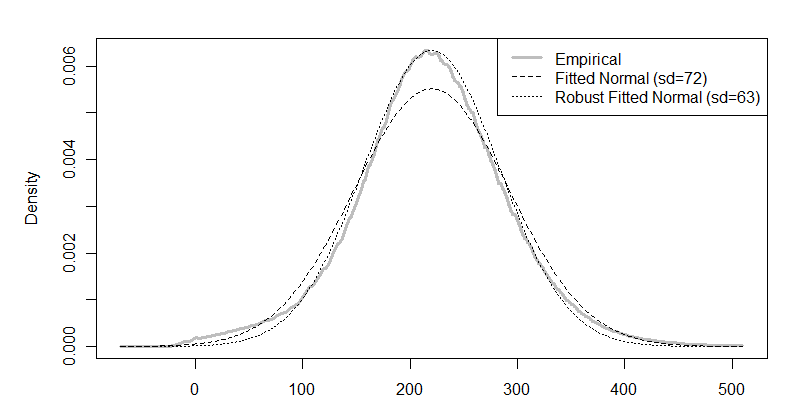
Figure 2: Empirical distribution of mapped insert sizes.

The proportion of hanging reads for these data is 3.3%, of which about 2% comes from pairs where one read is unmapped. The $\alpha=0.1$ threshold for $Z^{H}$, using $r=0.1$ and a stepsize of 10, is 10.26. The $\alpha=0.01$ threshold is 11.21

It is difficult to visualize such a massive data set. Figure 3 shows the scores $Z^{B}$ and $Z^{H}$ for a quite typical one megabase long region. Even at this resolution, the data are a blur. Overlayed on the plot for $Z^{B}$ are dashed lines, which represent the mean $+/-$ 3 standard deviations for the null distribution of the scores, which are computed analytically using our model. For $Z^{H}$ only the mean is shown, since this score is heavily skewed. Note that most of the $Z^{B}$ process lie within this band, and that the null mean for $Z^{H}$ does seem to be at the right place. Such visual checks give reassurance that the null model is a good approximation to the bulk of the data, and are an important part of the analysis. The solid lines in the plots represent the threshold for family-wise error rate of 0.1.

Figure 3: Insert length score $Z^{B}$ (top) and Minus strand hanging reads score $Z^{-}$ (bottom) scores for one megabase block on chromosome 20 of individual NA12878. The plus strand hanging reads score looks similar to $Z^{-}$ and is not shown.

Table 7 shows the number of calls made by the insert length statistic $Z^{B}$ and the hanging reads statistic ($Z^{+}$ or $Z^{-}$) on Chromosome 20, and the number of places where the calls seem to be supporting the same variant. For each score, overlapping windows where the score exceeds the threshold are merged into the same call. For $\alpha=0.1$, 634 calls were made by $Z^{B}$, 3211 were made by $Z^{+}$ and 2790 were made by $Z^{-}$. For $\alpha=0.01$, 399 calls were made by $Z^{B}$, 2935 were made by $Z^{+}$ and 2461 were made by $Z^{-}$. At each p-value, about 5-6 times more calls were made by the hanging reads statistics. This may be due to a higher number of false positives due to lack of robustness, a higher sensitivity of the hanging reads statistic for insertions and small deletions, or a combination of these factors. Without biological validation, it is hard to know. We expect a true deletion to generate a peak in $Z^{B}$, coupled with minus strand hanging reads at the left boundary and plus strand hanging reads at the right boundary. The number of regions called by $Z^{B}$ that overlap a call by $Z^{-}$ at the left end and a call by $Z^{+}$ at the right end is 58 for $\alpha=10\%$ and 47 for $\alpha=1\%$. This implies that only $10\%$ of calls made by the insert length statistic are supported by evidence from hanging reads. Although the small overlap is cause for concern, visual inspection of the calls made by $Z^{B}$ that were not supported by hanging reads suggest that many of these calls may be real; an example is shown below.

Method	$\alpha=10\%$ $\alpha=1\%$
I. Insert length ($Z^{B}$)	634	399
II. Minus strand hanging reads	3211	2935
III. Plus strand hanging reads	2790	2461
Overlap between I and (II and III) at ends ∗	58 ($9\%$)	47 ($12\%$)

Table 7: Number of calls made on NA12878 chromosome 20 by a scan using only the insert length statistic (I), only the minus strand hanging reads statistic (II), or only the plus strand hanging reads statistic (III). Results for two different FWER thresholds, $\alpha=10\%,1\%$ are shown. Row 4shows the number (and percentage) of regions from I that overlap with a region in II at the left end, and a region in III at the right end.

Figures 4 and 5 show two example regions where either one or both scores have passed the threshold. In Figure 4, there is a putative homozygous deletion of about 200 bases which generates the ideal pattern of a cluster of read pairs with shifted insert length preceding a region of no coverage (top plot). Supporting this deletion are peaks in both $Z^{+}$ and $Z^{-}$. (The bottom plot shows their sum.)

Figure 4: A region containing a putative homozygous deletion of roughly 200 base pairs on chromosome 20. Top plot shows the mapped insert length versus the start position of the plus strand read. Middle plot shows the insert length score in this region. Bottom plot shows $Z^{H}$, the hanging reads score.

Figure 5 shows a cluster of read pairs with roughly 800 bp shift in insert length preceding a region of approximately 800 base pairs with coverage reduced by about half. This visibly obvious tell tale pattern for a heterozygous deletion is convincing even without careful mathematical modeling. Yet, at the $\alpha=10\%$ level there are no significant peaks in either the plus or minus strand hanging read scores. Cases like this are not uncommon in the data. There are also cases where strong evidence from the hanging reads are not supported by evidence from $Z^{B}$. Real data is erratic, and ideal patterns like the example in Figure 4 are the exception rather than the rule.

Figure 5: A region containing a putative heterozygous deletion of roughly 800 base pairs on chromosome 20. Top plot shows the mapped insert length versus the start position of the plus strand read. Middle plot shows the insert length score in this region. Bottom plot shows $Z^{H}$, the hanging reads score.

The genome scan that produces a list of candidate regions is only one of many steps in the analysis of such a rich data set. To improve confidence and accuracy, regions such as those in Figures 4 and 5 should be analyzed more carefully, ideally by a more laborious local assembly of the reads that map to the region.

8 Summary and Discussion

We studied scan statistics for Poisson-type data, with emphasis on several statistics that are useful for detecting local genomic signals in next-generation sequencing experiments, such as peak detection in ChIP-Seq and structural variant detection by paired-end whole genome sequencing. Despite their different formulations, analytic significance approximations for these statistics can be obtained through a general framework that involves embedding the statistics into an exponential family (3.3) and applying the measure transformation technique described in Siegmund, Yakir and Zhang (2011). See also Yakir (2013).

Some of our analyses have been focused on a mixture model, which we characterized using the kernel function (3.6). This model can be viewed as a simplified version of the model for bracketing read pairs (3.11). (A simplified version of the hanging reads model is suggested in Remark 2 at the end of Section 3.3.) We described significance level approximations under this model in detail, and showed by Monte Carlo that they are reasonably accurate. We also conducted power studies under this model, which reveal a complex picture regarding how power depends on the choice of scanning parameter(s), the assumed homogeneity of the process, and the values of nuisance parameters. The key observations are summarized in Section 6.7. We expect these qualitative statements regarding power to generalize to the more complex models in Section 3.3, although some aspects neglected by the simplified models, e.g., the asymmetry between insertions and deletions, may fail to be accurately illustrated. For a numerical example, for parameters associated with the second row of Table 4, where the bracketing pairs statistic for our better model to detect insertions has marginal power 0.75, the simple mixture model would have power 0.93; the simplified model for hanging reads would have marginal power 0.85 compared to 0.95 for the better model.

For structural variant detection using paired-end sequencing, we formulated a model that incorporates three different features of the data: Read coverage, mapped insert length, and hanging read pairs. The log likelihood ratio scan statistic under this model is a sum of terms, which we call “scores,” for each of these three features. While the bracketing pairs statistics have increasing power to detect longer deletions, their power to detect insertions first increases, then decreases with the length of the insertion. The power of the hanging read statistics to detect deletions does not depend on the length of the deletion, while their power to detect insertions increases with the length of the insertion and approach an asymptote typically less than one.

Although read coverage is suggested as one source of information in our model, we have neglected it in the power calculations that we report in detail. The reason is that the read coverage statistic usually performs poorly unless the true value of $r$ is close to .5 and the deletion (for example) is fairly long; in which case the statistic using mapped insert length is itself reasonably powerful. If we use the sum of $Z^{C}$ and $Z^{B}$ to call deletions, for most alternatives we have smaller marginal power compared to using $Z^{B}$ alone, although in specific cases the marginal power does increase. For example, for rows 11-13 of Table 5, the marginal power would become 0.38, 0.91, and 0.43 respectively. For $r=0.4$ or 0.5 and $w=100$ or 150, the marginal power of the sum $Z^{C}+Z^{B}$ is greater than that for $Z^{B}$ alone, but then the marginal power of the hanging read statistic in these cases is even greater.

In the empirical data that we have examined, larger mean insert lengths also have substantially larger standard deviations. Also, such libraries tend to exhibit skewness and sometimes even multimodality. A consequence of the contemporary move to increase read and insert length is that relatively speaking the hanging read statistics gain power, but the bracketing pairs statistics can lose substantial power.

Our analyses in Section 7 assume constant read coverage $\kappa$. As mentioned in Section 3.3, mean read coverage has been empirically observed to fluctuate along the genome and correlates with known features such as GC content. Since the null distribution of the scores depend on $\kappa$, if we allow $\kappa$ to vary the thresholds for the scores would change with genome position. Even with the analytic approximations for the p-values, back-solving them to obtain appropriate thresholds for a given significance level requires a substantially increased amount oft computation. One could also conduct the scan using the corresponding likelihood ratios $\ell_{\tau}=\beta Z_{\tau}-\psi(\beta)$, the thresholds for which are much less variable as a function of $\kappa$. However, the parameter $\beta$ in the likelihood ratio statistic would vary with $\kappa$ and thus the computational issue can not be avoided. A viable option in practice is to first segment the genome into blocks of approximately homogeneous read coverage, then scan each block separately with a threshold computed using the block-specific $\kappa$. The global p-value would then be simply the sum of the block-wise p-values. In implementing this approach, one may want to ignore genomic regions of low coverage. One of the lessons of the simple mixture model is that a substantial amount of power is inevitably lost in regions of low coverage and cannot be recovered by a simple adjustment of the significance threshold.

An open question is how different statistics should be combined to improve detection accuracy. We found in our power analysis that summing the scores, as in the log-likelihood, is rarely better than applying each score individually. The reason is that for most alternative settings there is one score that dominates the others, and incorporating the others by simple addition contributes mainly noise. Thus, it may be better to apply each score individually and then combine detections using a Bonferroni correction. It may also be better to combine the scores in a weighted sum, as in Senbaobaglu, Li and Zhang (2011).

While we have been focusing mainly on control of the family-wise error rate, in genomic studies the false discovery rate (FDR) is often an appealing mode of multiple testing control. The boundary crossing probabilities can be easily converted into the expected number of false discoveries under the null, and used for FDR control as described in Siegmund, Yakir, and Zhang (2011).

REFERENCES

Abyzov, A., Urban, A., Snyder, M. and Gerstein, M. (2011). CNVnator: An approach to discover, genotype, and characterize typical and atypical CNVs from family and population genome sequencing. Genome Research 21, 974-984.

Benjamini, Y. and Speed, T.P. (2012). Summarizing and correcting the GC content bias in high-throughput sequencing. Nucleic Acids Research 40, e72.

Campbell, P. J., Stephens, P. J., Pleasance, E. D., O’Meara, S., Li, H., San- tarius, T., Stebbings, L. A., Leroy, C., Edkins, S., Hardy, C., Teague, J. W., Menzies, A., Goodhead, I., Turner, D. J., Clee, C. M., Quail, M. A., Cox, A., Brown, C., Durbin, R., Hurles, M. E., Edwards, P. A. W., Bignell, G. R., Stratton, M. R. and Futreal, P. A. (2008). Identification of somatically acquired rearrangements in cancer using genome-wide massively parallel paired-end sequencing. Nature Genetics 40, 722-729.

Chan, H.P. and Zhang, N. R. (2006). Scan statistics with weighted observations. J. of American Statistics Association 102, 595-602.

Chiang, D. Y., Getz, G., Jaffe, D. B., O’Kelly, M. J., Zhao, X., Carter, S. L., Russ, C., Nusbaum, C., Meyerson, M. and Lander, E. S. (2009). High-resolution mapping of copy-number alterations with massively parallel sequencing. Nature methods 6, 99-103.

Feingold, E., Brown, P. O., and Siegmund, D. (1993). Gaussian models for genetic linkage analysis using complete high resolution maps of identity by descent. Am. J. Hum. Genet. 53, 234-251.

Karlin, S., Dembo, A. and Kawabata, K. (1990). Statistical composition of high-scoring segments from molecular sequences. Annals of Statistics 18, 571-581.

Lander, E.S. and Botstein, D. (1989). Mapping mendelian factors underlying quantitative traits using RFLP linkage maps. Genetics 121, 185-199.

Medvedev P, Stanciu M, Brudno M. (2009) Computational methods for discovering structural variation with next generation sequencing. Nature Methods 6, S13-20.

Peng, Jie and Siegmund, D. (2005). The admixture model in linkage analysis, J. Statist. Planning and Inference 130, 317-324.

Rabinowitz, D. and Siegmund, D. (1997). The approximate distribution of the maximum of a smoothed Poisson random field, Statistica Sinica (1997) 7 167-180.

Schwartzman, A., Jaffe, A., Gavrilov, Y. and Meyer, C.E. (2013). Multiple testing of local maxima for detection of peaks in ChIP-seq data, Annals of Applied Statistics, 7, 471-494.

Shen, J. and Zhang, N. R. (2012). Change-point model on nonhomogeneous Poisson processes with application in copy number profiling by next-generation DNA sequencing. Annals of Applied Statistics 6, 476-496.

Siegmund, D. and Worsley, K. (1995). Testing for a signal with unknown location and scale in a stationary Gaussian random field, Ann. Statist. 23 608-639.

Siegmund, D., Yakir, B. and Zhang, N.R. (2010). Tail approximations for maxima of random fields by likelihood ratio transformations, Sequential Analysis. 29, 245-262.

Siegmund, D., Yakir, B. and Zhang, N.R. (2011). Detectiing simultaneous variant intervals in aligned sequences, Ann. Appl. Statist. 5 645-668.

Siegmund, D., Yakir, B. and Zhang, N.R. (2011). False discovery rate for scan statistics, Biometrika 98, 979-986.

Tang, H.K. and Siegmund, D. (2001). Mapping quantitative trait loci in oligogenic models, Biostatistics 2, 147-162.

Worsley, K.J., Evans, A.C., Marrett, S. and Neelin, P. (1992). A three dimensional statistical analysis for CBF activation studies in human brain, Journal of Cerebral Blood Flow and Metabolism 12, 900-918.

Yakir, B. (2013). Extremes in Random Fields: A Theory and Its Applications, Wiley, Chichester, United Kingdom.