On non-disk geometry of in Kerr-de Sitter
and Kerr-Newman-de Sitter spacetimes
Abstract
Gaussian curvature of the two-surface , is calculated for the Kerr-de Sitter and Kerr-Newman-de Sitter solutions, yielding non-zero analytical expressions for both the cases. The results obtained, on the one hand, exclude the possibility for that surface to be a disk and, on the other hand, permit one to establish a correct geometrical interpretation of that surface for each of the two solutions.
pacs:
04.20.Jb, 04.70.Bw, 97.60.LfI Introduction
It is well known that the two-surface , of the Kerr solution Ker has zero Gaussian curvature ONe1 and therefore is commonly interpreted as a disk BLi ; HEl or a “flat sphere” composed of two disks of radius joined together along the ring singularity ONe2 . For not quite perspicuous reasons, these interpretations had been automatically extrapolated to the analogous surfaces in generalized Kerr black-hole spacetimes involving electromagnetic field or cosmological constant, as may be readily inferred by examining for instance the Penrose-Carter conformal diagrams of the Kerr-Newman (KN) or Kerr-de Sitter (KdS) spacetimes NCC ; Car1 ; GHa where the regions of positive and negative radial coordinate are supposedly glued on such disks. Recently, however, using a direct calculation GCM , the Gaussian curvature of the surface , in the KN case has been shown to be a function of the polar coordinate , thus clearly disproving the disk interpretation of the latter surface in that case. Moreover, a study of the above two-surface in the Weyl-Papapetrou cylindrical coordinates carried out in the same paper GCM has resulted in a novel interpretation of that surface even in the case of the Kerr solution – a dicone instead of a disk – which looks plausible since a dicone is a closed surface having, like a disk, zero Gaussian curvature and in addition better fitting the corresponding surface’s equation in cylindrical coordinates.
The present communication is aiming, firstly, to provide convincing evidence against the disk interpretation of the surface , in the case of two well-known black-hole solutions with a non-zero cosmological constant, namely, the KdS and Kerr-Newman-de Sitter (KNdS) spacetimes Car1 ; GHa ; Car2 , and, secondly, to establish a correct geometrical interpretation of that important surface and briefly discuss the main mathematical and physical implications engendered by the new geometry.
II The surface , in KdS spacetime
The KdS metric was obtained by Carter, and in the Boyer-Lindquist-like coordinates it has the form
| (1) |
where
| (2) |
the parameters and being related to the mass and angular momentum per unit mass of the source, and being the cosmological constant. The ring singularity of this spacetime corresponds to , .
Since our interest lies basically in establishing the geometry of the surface , , we are not going to touch here the general properties of the KdS solution, restricting ourselves to only mentioning that their discussion can be found, e.g., in the papers GHa ; AMa and monograph GPo . With that said, we go directly to the two-surface we are interested in and write out its line element,
| (3) |
which does not contain the mass parameter .
To calculate the Gaussian curvature of the surface (3) which equals half the scalar curvature , we have used an utterly user-friendly computer program “Ricci” Agu and obtained the following very simple formula
| (4) |
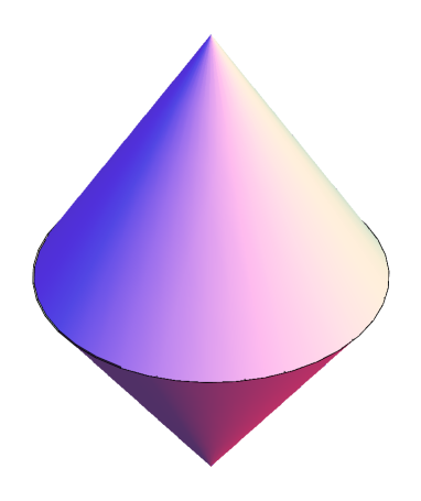
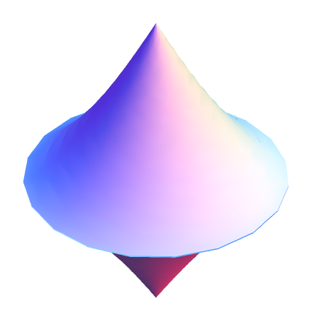
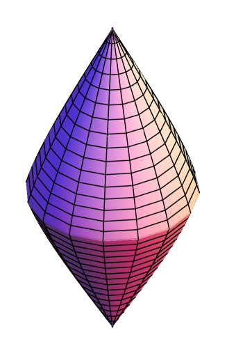
Though it is tempting to conclude from (4) that the surface (3) is a sphere or a pseudosphere depending on whether or , such a conclusion would not be really correct since, for instance, Liebmann’s theorem on the closed surfaces with positive is applicable to regular surfaces only. At the same time, as it follows from (3), our two-surface has a singularity at (it is the ring singularity of KdS solution), and it may also be non-regular at the points and . It is clear as well that in the case the surface of negative Gaussian curvature cannot be a tractricoid because the latter then would have been stretching along the entire symmetry axis. Taking into account that the , surface of the Kerr solution () is a dicone depicted in Fig. 1, it would be plausible to suppose that in the Kerr-anti-de Sitter case the respective surface is represented by some conic surface of a constant negative Gaussian curvature with singular vertices and equator, like the one shown in Fig. 2. By analogy, the surface , of the KdS solution with is represented by a conic surface of rotation with constant positive Gaussian curvature and singular vertices and equator (see Fig. 3). For the theory of such surfaces and practical aspects of their construction we refer the reader to the monograph Gra .
The surfaces from figures 2 and 3, which we shall dub, respectively, a concave dicone and a convex dicone of constant Gaussian curvature, are remarkable in several regards. First of all, and most importantly, they leave no doubt that the surface , of the KdS solution is not a disk. Moreover, they provide a strong support to the novel interpretation of the above surface in the Kerr solution – a dicone of zero Gaussian curvature – which may be considered as the simplest () non-trivial specialization of the general KdS case. It is also surprising that the cosmological constant in the KdS metric modifies the surface , of the pure Kerr spacetime in such a way that the Gauss curvature of that surface in the presence of still remains constant, something that does not happen, as will be seen in the next section, when a charge parameter is introduced into the solution.
III The surface , in KNdS spacetime
The charged version of the KdS field, the KNdS solution, was also obtained by Carter, but its conventional form currently used in the literature is due to the paper of Gibbons and Hawking GHa ; the solution is determined by the line element
| (5) |
where
| (6) |
and is the charge parameter. The associated electromagnetic four-potential is given by
| (7) |
Compared to the metric (1), the line element (5) contains the factor appearing as a result of rescaling the coordinates and ; however, as will be seen below, this factor does not affect anyhow the intrinsic geometry of the surface , .
The latter two-surface is defined by the line element
| (8) |
and the corresponding Gaussian curvature can be shown to have the form
| (9) | |||||
By setting in (9), one recovers the constant value (4) of the KdS solution, thus demonstrating that the rescaling factor does not modify the Gaussian curvature of the surface under consideration, and in the limit one arrives at the respective of the KN space obtained in GCM :
| (10) |
Comparison of formulas (4), (9) and (10) leads to a conclusion that the effect of the charge parameter on the geometry of the surface , of the Kerr solution is more significant than the analogous effect produced by the cosmological constant , and also that the combined effect of the parameters and distorts drastically that surface. It has already been shown in GCM that formula (10) defines a specific surface of revolution of positive and negative Gaussian curvature; in this respect, the surface determined by (9) must in fact be given exactly the same interpretation as in the KN case, with the only additional remark that obviously the particular form of the regions of positive and negative Gaussian curvature defined by zeros of the numerator in (9) cannot be studied analytically, needing a numerical analysis. Therefore, one can see that the surface , of the KNdS solution cannot be interpreted as a disk, rather being a surface of revolution with various regions of positive and negative Gaussian curvature dependent on the polar coordinate . We leave to the reader’s imagination the task of deforming (in the equatorially symmetric manner) the dicones from Figs. 2 and 3 for having an idea of how that surface may look like for positive and negative values of .
IV Discussion
The established fact that the surface , in the KdS and KNdS solutions is not a disk has several mathematical and physical consequences. First of all, it is now obvious that, if , the usual Boyer-Lindquist-like coordinates do not cover the whole KdS and KNdS manifolds, leaving the interior regions of dicones beyond their attainability. In this respect, the above surface of a stationary black hole cannot be considered as its center, contrary to what was suggested in ONe2 , as it is apparent that the black hole’s center must coincide with the geometrical center of the ring singularity, which is also the geometrical center of a concrete dicone containing that singularity.
The non-disk geometry of the surface , seems to invalidate the known approaches to the extensions of the black-hole rotating spacetimes to infinite negative values of the radial coordinate requiring an artificial gluing of the spaces with and on the “disks”. Indeed, the supposition that this surface is a disk (in a non-extended spacetime, to avoid confusion) implies that the disk lies in the equatorial plane, so that by crossing it from the upper hemisphere (), one immediately finds oneself in the other hemisphere (). However, if the above surface is represented by any of the dicones considered in the previous section, then by crossing a dicone at some , one still will be staying in the same hemisphere, apparently needing to cover some distance in order to reach the equatorial plane; by crossing the latter, one will find oneself in the second hemisphere still inside the dicone, and will need to run another way for being able to eventually go out of the dicone at some . The interior of the dicone can be appended to the general manifold corresponding to in various ways, for instance by redefining the radial coordinate in the manner suggested in GCM for the KN solution, which would be equivalent to extending to a finite negative value (the possibility discussed in MRu ), or by introducing an appropriate set of coordinates fully covering the regions exterior and interior to the dicone’s surface. Concerning the latter possibility it is worth remarking that the introduction of a new coordinate set may in principle depend on the sign of the mass parameter , like it takes place, e.g., in the case of the KN solution whose exterior and interior regions are rather well described by the usual Weyl-Papapetrou cylindrical coordinates only when GCM ; MRu . Incidentally, in the presence of a non-zero cosmological constant the problem of introducing the Weyl-Papapetrou-like coordinates in the stationary axisymmetric solutions is more complicated than in the case and is likely to be studied in more detail in the future (an important work in this direction has been recently done in CLS ; Ast ).
Though it is clear that the surface , is not smooth and therefore an analytic extension through it may exhibit problems of differentiability (that is why a set of coordinates better than that of Boyer and Lindquist is actually needed), one still could ask oneself a question about an exact negative value of the aforementioned finite at which the center of the ring singularity will be attained during the extension procedure through the dicone’s surface by using directly the Boyer-Lindquist coordinates. This question is not as trivial as may look like, and at the moment we cannot give an exhaustive answer to it. At the same time, taking into account that the Gauss curvature of a sphere is , being singular at , it might look plausible as a possibility to associate the center of the ring singularity of the KdS and KNdS black-hole solutions with one of the singularities of the Gaussian curvature of the corresponding surface , . While the calculation of for the latter surface does not represent technical difficulties, the resulting expression, however, is very cumbersome and we do not give it here. Instead, we write out below the form of that in the particular case when the general expression considerably simplifies, yielding
| (11) |
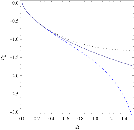
The above formula describes Gaussian curvatures of the surfaces , of the KNdS solution at the points located in the equatorial plane, and the apparent singularity at corresponds to the usual ring singularity , . Therefore, starting from some positive and moving in the equatorial plane towards the center, one first comes to the singular point and then, after passing it, finds oneself in the zone of negative inside the region enclosed by the surface , . The second factor in the denominator of (11) is a quartic polynomial in ; then, if we set for simplicity , this factor further factorizes into and , the latter having the following real negative root when , :
| (12) |
In figure 4 we have plotted a characteristic dependence of on for the particular value of the mass parameter and three different values of : (these correspond to dashed, solid and dotted lines, respectively), whence it follows that is an increasing function of , and also that for a given value of the respective is the largest in the case of negative . At the same time, the question whether the above really represents the center of the ring singularity still may require further clarification.
The main physical implication of our results consists in giving a fairly new picture of the internal structure of rotating black holes in the vicinity of the ring singularity. As a matter of fact, it is clear now that in an appropriate coordinate atlas fully covering the regions exterior and interior to the closed conic surfaces of revolution the ring singularity will be smoothly traversable by the observers who may cross it from one hemisphere to another in any direction as many times as they like, always staying in the same black-hole spacetime – no introduction of an additional copy of the solution with another spatial infinity for artificially attaching it to the non-smooth surface , is required.
Acknowledgments
This work was partially supported by Project 128761 from CONACyT of Mexico.
References
- (1) R. P. Kerr, Phys. Rev. Lett. 11, 237 (1963).
- (2) B. O’Neill, Elementary Differential Geometry (Academic Press, New York, 1966).
- (3) R. H. Boyer and R. W. Lindquist, J. Math. Phys. 8, 265 (1967).
- (4) S. W. Hawking and G. F. R. Ellis, The Large Scale Structure of Space-Time (Cambridge Univ. Press, 1973).
- (5) B. O’Neill, The Geometry of Kerr Black Holes (A. K. Peters, Wellesley, Massachusetts, 1995).
- (6) E. Newman, E. Couch, K. Chinnapared, A. Exton, A. Prakash and R. Torrence, J. Math. Phys. 6, 918 (1965).
- (7) B. Carter, in: Black Holes (Gordon and Breach, New York, 1973) p. 56.
- (8) G. W. Gibbons and S. W. Hawking, Phys. Rev. D 15, 2738 (1977).
- (9) H. García-Compeán and V. S. Manko, ArXiv:1205.5848 v.5 [gr-qc] (2014).
- (10) B. Carter, Commun. Math. Phys. 10, 280 (1968).
- (11) S. Akcay and R. A. Matzner, Class. Quantum Grav. 28, 085012 (2011).
- (12) J. B. Griffiths and J. Podolský, Exact Space-Times in Einstein’s General Relativity (Cambridge Univ. Press, 2009).
- (13) J. M. Aguirregabiria, Computer program “Ricci”, 2002.
- (14) A. Gray, Modern Differential Geometry of Curves and Surfaces (CRC Press, Boca Raton, 1993).
- (15) V. S. Manko and E. Ruiz, Prog. Theor. Exper. Phys. 2013, 103E01 (2013).
- (16) C. Charmousis, D. Langlois, D.A. Steer and R. Zegers, JHEP 02, 064 (2007).
- (17) M. Astorino, JHEP 06, 086 (2012).