Universal Order Parameters and Quantum Phase Transitions: A Finite-Size Approach

Abstract

We propose a method to construct universal order parameters for quantum phase transitions in many-body lattice systems. The method exploits the $H$-orthogonality of a few near-degenerate lowest states of the Hamiltonian describing a given finite-size system, which makes it possible to perform finite-size scaling and take full advantage of currently available numerical algorithms. An explicit connection is established between the fidelity per site between two $H$-orthogonal states and the energy gap between the ground state and low-lying excited states in the finite-size system. The physical information encoded in this gap arising from finite-size fluctuations clarifies the origin of the universal order parameter. We demonstrate the procedure for the one-dimensional quantum formulation of the $q$-state Potts model, for $q=2,3,4$ and 5, as prototypical examples, using finite-size data obtained from the density matrix renormalization group (DMRG) algorithm.

Order parameters are pivotal to the Landau-Ginzburg-Wilson description of phase transitions for a wide range of critical phenomena, both classical and quantum, in many-body systems arising from spontaneous symmetry breaking (SSB).SSB ; Anderson Despite their importance, relatively few systematic methods for determining order parameters have been proposed. One method proposed for quantum many-body lattice systems utilizes reduced density matrices.FMO This approach takes advantage of the degenerate ground states (GSs) which appear when a symmetry of the Hamiltonian is broken spontaneously in the thermodynamic limit. An order parameter can be identified with an operator that distinguishes the degenerate GSs. The idea of the method is to search for such an operator by comparing the reduced density matrices of the degenerate GSs for various subareas of the system. This method was demonstrated in models that are considered to exhibit dimer, scalar chiral, and topological orders.FMO

Another approach makes use of the ground-state fidelity of a quantum many-body system.FID ; LAD ; KIT For a quantum phase transition (QPT) arising from SSB, a bifurcation appears in the ground-state fidelity per lattice site, with a critical point identified as a bifurcation point.bif This in turn results in the concept of the universal order parameter (UOP),UOP in terms of the fidelity per site between a ground state and its symmetry-transformed counterpart. The advantage of the UOP over local order parameters in characterizing QPTs is that the UOP is model independent, and thus universal, in sharp contrast with local order parameters, which are usually determined in an ad hoc fashion.

UOPs have been calculated with tensor network (TN) algorithms for systems with translational invariance. For Hamiltonians possessing symmetry group $G$ with $g$ the element of $G$, UOPs for translational invariant infinite-size systems are defined based on the orthogonal degenerate GSs corresponding to SSB, as a measure of distinguishability between ground state $|\psi\rangle$ and quantum state $g|\psi\rangle$, which can be interpreted in terms of the fidelity $F$ as a measure of the similarity between two states.NILSEN

Such UOPs satisfy the basic definition of an order parameter: namely in the SSB phase, with $|\psi\rangle$ and $g|\psi\rangle$ two of the degenerate GSs, the corresponding UOP is nonzero, whilst in the symmetric phase, with $g|\psi\rangle\equiv|\psi\rangle$, the UOP is zero. It has been demonstrated that such UOPs can successfully describe the symmetry broken phases in both one-dimensional and two-dimensional quantum systems. UOP ; UOP2D

Since SSB occurs only in the thermodynamic limit, this construction of UOPs only makes sense in infinite-size quantum many-body systems. It is clearly desirable however, to construct UOPs directly from finite-size systems. This will not only make it possible to perform finite-size scaling, but also make it possible to take full advantage of currently available numerical algorithms, such as quantum Monte Carlo,MC finite-size density matrix renormalization group (DMRG),DMRG and finite-size TN algorithms.TN Here we propose and test a specific scheme to do this in the finite-size context for systems with SSB.

Construction of UOPs from $H$-orthogonal states.– First, we recall the notion of fidelity per lattice site. The fidelity $F(|\varphi_{1}\rangle,|\varphi_{2}\rangle)=|\langle\varphi_{1}|\varphi_{2}\rangle|$ between two states $|\varphi_{1}\rangle$ and $|\varphi_{2}\rangle$ scales as $F(|\varphi_{1}\rangle,|\varphi_{2}\rangle)\sim d(|\varphi_{1}\rangle,|\varphi_{2}\rangle)^{L}$, with $L$ the number of lattice sites. The fidelity per lattice site FID $d$ is the scaling parameter

$$\ln{d(|\varphi_{1}\rangle,|\varphi_{2}\rangle)}\equiv\lim_{L\rightarrow\infty}\frac{\ln F(|\varphi_{1}\rangle,|\varphi_{2}\rangle)}{L},$$ (1)

which is well defined in the thermodynamic limit. With $|\varphi_{1}\rangle$ and $|\varphi_{2}\rangle$ ground states for different values of the control parameter, the fidelity per lattice site is nothing but the partition function per site in the classical statistical lattice model.PAT

We consider a hamiltonian $H$ of a quantum system possessing symmetry group $G$ with $g$ a unitary representation of $G$, i.e., $U^{g}H{U^{g}}^{\dagger}=H$, with $U^{g}=g\otimes g\otimes g\ldots$ an infinite string of copies of matrix $g$. With the SSB, the UOP is defined in terms of the fidelity per lattice site $d_{\infty}$ for an infinite-size system bynote1

$${\cal O}=\sqrt{1-d_{\infty}^{2}}\,,$$ (2)

where $d_{\infty}=|\langle\psi|g|\psi\rangle|^{1/L}$ with $L\rightarrow\infty$ the fidelity per lattice site between the ground state $|\psi\rangle$ and the quantum state $g|\psi\rangle$.UOP ; UOP2D

To study UOPs in the finite-size context, it is natural to think of using the fidelity per lattice site $d_{L}$ for systems of finite size $L$ to construct $d_{\infty}=\lim_{L\rightarrow\infty}{d_{L}}$. However, applying the same definition of $d_{L}$ with the GSs of a finite-size system fails because $d_{\infty}\equiv 0$ in all the range for $|\langle\psi|g|\psi\rangle|^{1/L}=0$ in both phases, as SSB occurs only in an infinite-size system. There is however, a way to overcome this obstacle for finite-size systems.

To outline the general idea, consider a system whose hamiltonian has $Z_{q}$, $q\in\mathbb{Z}^{+}$ symmetry. At zero temperature, for the symmetry broken phase, we have $q$ degenerate ground states in the thermodynamic limit and we do expect that the symmetry is spontaneously broken. First we calculate $q$ low-lying states of this system with finite size $L$, denoting the $i$th eigenstate and corresponding eigenvalue by $|\phi_{i}\rangle$ and $E_{i}$, satisfying $H|\phi_{i}\rangle=E_{i}|\phi_{i}\rangle$. The $Z_{q}$ symmetry can be understood as rotations among the variables pointing in the corresponding field directions. Thus the Hilbert space associated with $Z_{q}$ can be separated into disjoint sectors labeled by the phases $\omega_{m}=\exp{(2\pi i(m-1)/q)}$ with $m=1,2,\ldots,q$. For our purpose, we construct $q$ $H$-orthogonal states $|\psi_{m}\rangle$ from the $q$ low-lying states $|\phi_{m}\rangle$ by

$$|\psi_{m}\rangle=\sum_{j}{\omega_{m}^{j-1}c_{j}\,|\phi_{j}\rangle},$$ (3)

in terms of the above defined phases $\omega_{m}$.

Here, each pair of the $q$ states are set to be orthogonal with respect to $H$, i.e.,

$$\langle\psi_{m}|H|\psi_{t}\rangle=0,$$ (4)

with $m\neq t$, so called $H$-orthogonality.note2 The $q$ coefficients $c_{j}$ are fixed by the $H$-orthogonality and normalization conditions. The fidelity per lattice site of two $H$-orthogonal states $|\psi_{t}\rangle$ and $|\psi_{m}\rangle$ takes the form

$$d_{L}=|\langle\psi_{m}|\psi_{t}\rangle|^{1/L}=\left|\sum_{j}{\omega_{t-m}^{j-1}|c_{j}|^{2}}\right|^{1/L}.$$ (5)

The final step in the scheme is to extrapolate the fidelity per lattice site $d_{L}$ between two $H$-orthogonal states, $d_{\infty}=\lim_{L\rightarrow\infty}{d_{L}}$, with the UOP following from the definition in Eq. (2). This explains how degenerate GSs in the thermodynamic limit, responsible for symmetry breaking order, emerge from near degenerate low-lying states in the finite-size system.

Application: the $q$-state Potts model.– The quantum formulation of the $q$-state Potts model has hamiltonianqPotts

$$\small H=-\sum_{i}{\left(\sum_{\alpha=1}^{q-1}{M_{i}^{\alpha}M_{i+1}^{q-\alpha}}+\lambda M_{i}^{z}\right)}\,,$$ (6)

where $i$ are the lattice sites and $\lambda$ denotes the external field along the $z$ direction. The operators are written in matrix form:

$$M^{1}=\begin{bmatrix}0&I_{q-1}\\ 1&0\end{bmatrix},\quad M^{z}=\begin{bmatrix}q-1&0\\ 0&-I_{q-1}\end{bmatrix}$$ (7)

with $M^{i}=(M^{1})^{i}$ for $i=1,\ldots,q-1$, where $I_{q}$ is the $q\times q$ identity matrix. The hamiltonian has $Z_{q}$ symmetry. For $\lambda<1$ the system is in the $Z_{q}$ symmetry broken ferromagnetic phase, and a symmetric paramagnetic phase when $\lambda>1$. It is well known that a continuous (discontinuous) QPT occurs for $q\leq 4$ ($q>4$) at $\lambda=1$ where the model is exactly solved. baxter ; hamer

Consider first the case $q=2$, the quantum transverse Ising model, where matrices $M^{1}$ and $M^{z}$ are the Pauli matrices $\sigma^{x}$ and $\sigma^{z}$. Here the continuous QPT at $\lambda=1$ is between the $Z_{2}$ symmetry broken ferromagnetic phase and the symmetric paramagnetic phase. We compute the ground state wave function $|\phi_{gs}\rangle$ and the first excited state wave function $|\phi_{ex1}\rangle$ for a system with finite size $L$, with corresponding ground state energy $E_{gs}$ and first excited state energy $E_{ex1}$. Substituting $\omega_{1}=1$ and $\omega_{2}=-1$ into Eq. (3) gives the two $H$-orthogonal states

$$|\psi_{1}\rangle = c_{1}|\phi_{gs}\rangle+c_{2}|\phi_{ex1}\rangle,$$ (8)

$$|\psi_{2}\rangle = c_{1}|\phi_{gs}\rangle-c_{2}|\phi_{ex1}\rangle,$$ (9)

which satisfy the $H$-orthogonality and normalization conditions $\langle\psi_{1}|H|\psi_{2}\rangle=0$ and $\langle\psi_{1}|\psi_{1}\rangle=\langle\psi_{2}|\psi_{2}\rangle=1$. Thus, equivalently, we get

$$|c_{1}|^{2}E_{gs}-|c_{2}|^{2}E_{ex1}=0,$$ (10)

$$|c_{1}|^{2}+|c_{2}|^{2}=1,$$ (11)

with solution $|c_{1}|^{2}=E_{ex1}/(E_{gs}+E_{ex1})$ and $|c_{2}|^{2}=E_{gs}/(E_{gs}+E_{ex1})$. The fidelity per lattice site between the two $H$-orthogonal states is thus

$$d_{L}=\langle\psi_{1}|\psi_{2}\rangle|^{1/L}=\left||c_{1}|^{2}-|c_{2}|^{2}\right|^{1/L}=\left|\frac{\delta_{L}}{E_{gs}+E_{ex1}}\right|^{1/L},$$ (12)

with energy gap $\delta_{L}=E_{ex1}-E_{gs}$.

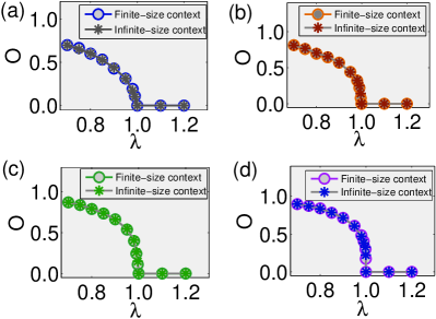
Figure 1: (color online): Comparison of UOPs ${\cal O}$ for the $q$-state quantum Potts model for $q=2,3,4$ and $5$ shown in $(a)$, $(b)$, $(c)$ and $(d)$, respectively. In each case the UOP is calculated from finite-size systems and compared with the value obtained in the infinite-size context.

In a similar fashion we have constructed the UOPs from the $q$ low-lying states of the $q=3,4$ and 5-state quantum Potts model. The $q-1$ excited states share the same energy $E_{ex}$ above the ground state $E_{gs}$. Proceeding as for the $q=2$ case, the coefficients $c_{j}$ in Eq. (3) ensuring the $H$-orthogonality (Eq. (4)) and normalization conditions are obtained, with the expression for the fidelity per lattice site now

$$d_{L}(\lambda)=\left|\frac{\delta_{L}(\lambda)}{(q-1)E_{gs}(\lambda)+E_{ex}(\lambda)}\right|^{1/L},$$ (13)

where $\delta_{L}(\lambda)=E_{ex}(\lambda)-E_{gs}(\lambda)$. As such we have established an explicit connection between the fidelity per site between two $H$-orthogonal states and the energy gap between the ground state and low-lying excited states, which in turn renders clear physical implication for the UOP. We emphasize that each pair of $H$-orthogonal states shares the same value of $d_{L}$ for given $\lambda$.

For values of the transverse field in the range $0.7\leq\lambda\leq 1.3$, we calculated the fidelity per lattice site $d_{L}(\lambda)$ between the $H$-orthogonal states for finite-size systems $L$ ranging from 10 to 500 using the DMRG algorithm. We obtained $d_{\infty}(\lambda)$ and thus the UOP for each value of $\lambda$ by simple extrapolation with $d_{L}(\lambda)=d_{\infty}(\lambda)+\alpha L^{-\beta}$.

Fig. 1 shows the UOPs obtained for $q=3,4$ and 5 for values of the transverse field in the range $0.7\leq\lambda\leq 1.3$ from finite-size systems $L$ ranging from 10 to 500 using the DMRG algorithm. Also shown for comparison are the results obtained for infinite-size translation-invariant systems with the infinite time-evolving block decimation (iTEBD) algorithm.itebd The UOPs obtained from the finite-size approach outlined here and the infinite-size approach match with a relative difference of less than $2.5$ percent, which indicates the success of our scheme. In general, as also shown in Fig. 1, the UOP is seen to be capable of characterizing the nature of the quantum phase transition. For $q=2,3$ and 4 there is a continuous phase transitions at $\lambda=1$, whilst for $q=5$ the first-order (discontinuous) phase transition can be seen at $\lambda=1$. Here we remark that the fidelity per site has been demonstrated to be capable of detecting the discontinuous phase transitions in this model through the so-called multiple bifurcation points.fidPotts

Scaling.– For the $q$-state Potts model, the $q$ low-lying eigenstates are the single ground state and $q-1$ degenerate first excited states. The energy gap $\delta_{L}$ for a system of finite size $L$ obeys the relation $\delta_{L}\sim d_{L}^{L}$ as Eq. (13) indicates. In the SSB phase with $\lambda<1$ away from the phase transition point, the eigenspectrum is gapful and the energy gap $\delta_{L}$ is related to the correlation length $\xi_{L}$ by $\delta_{L}\sim\exp{(-L/2\xi_{L})}$. Taking $L\rightarrow\infty$, the fidelity per lattice site $d_{\infty}$ and correlation length $\xi_{\infty}$ are expected to be related by

$$\xi_{\infty}=-\frac{1}{2}\frac{1}{\ln{d_{\infty}}}.$$ (14)

Fig. 2 shows this expected relation between $d_{\infty}(\lambda)$ and $\xi_{\infty}(\lambda)$ for different values of $\lambda$. Here, the data are mainly obtained using the iTEBD algorithm for infinite-size systems. The results are consistent with the relation (14) holding throughout the SSB phase $\lambda<1$.

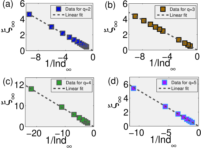
Figure 2: The effective relation between the correlation length $\xi_{\infty}$ and the UOP. In each case we calculate the correlation length $\xi_{\infty}(\lambda)$ and UOP ${\cal O}(\lambda)$ for control parameter $\lambda<1$ then fit $\xi_{\infty}(\lambda)$ and $\ln{d_{\infty}(\lambda)}$ to the relation $\xi_{\infty}=-a/\ln{d_{\infty}}$, with $d_{\infty}(\lambda)=\sqrt{1-{\cal O}(\lambda)^{2}}$. A simple linear fit gives the values (a) $a=-0.503$, (b) $a=-0.49$, (c) $a=-0.491$ and (d) $a=-0.506$.

At the critical point $\lambda=1$, the correlation length $\xi$ and energy gap $\delta_{L}$ scale as $\xi\sim 1/\delta_{L}$. With scale invariance at criticality, $\xi\sim L$, and thus $\delta_{L}\sim 1/L$. Then with $d_{L}^{L}\sim\delta_{L}$ the expected relation between the fidelity per site of the $H$-orthogonality states and finite size $L$ at criticality is $\ln{d_{L}}\sim-\ln{L}/L$. The results presented in Fig. 3 indicate that this relation is more precisely

$$\ln{d_{L}}\simeq-2\ln{L}/L.$$ (15)

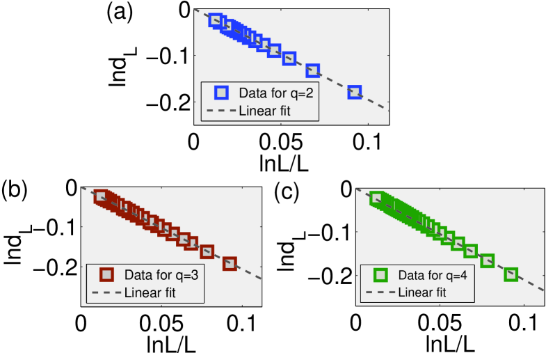
Figure 3: Finite-size scaling of the fidelity per site $d_{L}$ at criticality. In each case we fit $\ln{d_{L}}$ as a linear function of $\ln{L}/L$ and identify the amplitude $b$ with data for system size $L$ ranging from $50$ to $500$. The results are (a) $b=-1.96$, (b) $b=-2.06$ and (c) $b=-2.06$.

At the same time, keeping enough states with the DMRG algorithm, we have accurately obtained the gap $\Delta$ between the ground state and the $(q+1)$-th lowest state at criticality.note3 Here it is known that $\Delta\,\xi={\rm constant}$, which can be seen in the results of Fig. 4. The case $q=5$ is particularly challenging because the mass gap is small, with the exact value $\Delta=0.0020544\ldots$.hamer ; gap

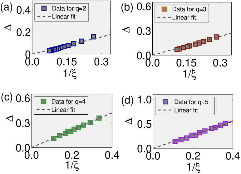
Figure 4: Physical gap $\Delta$ vs correlation length $\xi$ for the $q$-state quantum Potts model at criticality. For systems size $L$ ranging from 40 to 300, and a maximum number of 240 states kept during simulations with the DMRG algorithm, we fit the data to $\Delta\,\xi={\rm constant}$. For $q=5$ a finite gap is obtained by extrapolating with finite truncation dimension from the iTEBD algorithm. In each case convergence is expected towards the origin. However, at $q=5$ the mass gap terminates at the exact value $\Delta=0.0020544\ldots$.

Conclusions.— We have introduced a scheme for constructing UOPs to investigate QPTs using a set of $H$-orthogonal states in finite-size systems. We have established an explicit connection between the fidelity per site between two $H$-orthogonal states and the energy gap between the ground state and low-lying excited states in the finite-size system, which clarifies the physical meaning of the UOP. This makes it possible to perform finite-size scaling and take full advantage of currently available numerical algorithms. The scheme has been tested for the $q-$state quantum Potts model with $q=2,3,4$ and 5 using the finite-size DMRG algorithm. We have demonstrated that the UOPs obtained in the finite-size context agree with the UOPs obtained directly from the infinite-size context (Fig. 1). Our results suggest that, in the range where SSB occurs, the $H$-orthogonal states defined and obtained in finite-size systems correspond to the $q$ degenerate ground states for the infinite system when system size $L\rightarrow\infty$. This clarifies how degenerate GSs emerge in the thermodynamic limit from low-lying near-degenerate states through $H$-orthogonality. The UOPs we have thus defined are a further application of the fidelity per site in the characterisation of QPTs.

Furthermore, the general relation (14) between the correlation lengths and the fidelity is seen to hold in the SSB phase. At criticality we have established the result (15) for the scaling of the fidelity per site. Although we have considered UOPs from the point of view of finite-size systems with $Z_{q}$ symmetry breaking, it is anticipated that the scheme outlined here can also be extended and applied to any system undergoing a phase transition characterized in terms of SSB.

This work is supported in part by the National Natural Science Foundation of China (Grant Nos. 11174375 and 11374379) and by Chongqing University Postgraduates’ Science and Innovation Fund (Project No. 200911C1A0060322). M.T.B. acknowledges support from the 1000 Talents Program of China.

References

- (1) L. D. Landau, E. M. Lifshitz and E. M. Pitaevskii, Statistical Physics (Butterworth-Heinemann, New York, 1999).
- (2) P.W. Anderson, Basic Notions of Condensed Matter Physics (Westview Press, Boulder, 1997).
- (3) S. Furukawa, G. Misguich and M. Oshikawa, Phys. Rev. Lett. 96, 047211 (2006).
- (4) H.-Q. Zhou and J.P. Barjaktarevic̆, J. Phys. A 41, 412001 (2008); H.-Q. Zhou, J.-H. Zhao and B. Li, J. Phys. A 41, 492002 (2008); J.-H. Zhao, H.-L. Wang, Bo Li and H.-Q. Zhou, Phys. Rev. E 82, 061127 (2009); B. Li, S.-H. Li and H.-Q. Zhou, Phys. Rev. E, 79, 060101R (2009).
- (5) J.-H. Zhao and H.-Q. Zhou, Phys. Rev. B 80, 014403 (2009).
- (6) S.-H. Li, Q.-Q. Shi, Y.-H. Su, J.-H. Liu, Y.-W. Dai and H.-Q. Zhou, Phys. Rev. B 86, 064401 (2012).
- (7) H.-L. Wang, J.-H. Zhao, B. Li and H.-Q. Zhou, J. Stat. Mech.: Theory Exp. L10001 (2011); H.-L. Wang, Y.-W. Dai, B.-Q. Hu and H.-Q. Zhou, Phys. Lett. A 375, 4045 (2011); H-L. Wang, A-M. Chen, B. Li and H-Q. Zhou, J. Phys. A 45, 015306(2012).
- (8) J.-H. Liu, Q.-Q. Shi, H.-L. Wang, J. Links and H.-Q. Zhou, Phys. Rev. E 86, 020102(R) (2012).
- (9) M. A. Nielsen and I. L. Chuang, Quantum Computation and Quantum Information (Cambridge University Press, Cambridge, 2000).
- (10) S.-H. Li, H.-L. Wang, Q.-Q. Shi and H.-Q. Zhou, arXiv:1105.3008.
- (11) D.M. Ceperley and B.J. Alder, Phys. Rev. Lett. 45, 566 (1980).
- (12) S.R. White, Phys. Rev. Lett. 69, 2863 (1992); Phys. Rev. B 48, 10345 (1993); U. Schollwoeck, Rev. Mod. Phys. 77, 259 (2005).
- (13) G. Vidal, Phys. Rev. Lett. 91, 147902 (2003); Phys. Rev. Lett. 93, 040502 (2004); F. Verstraete, D. Porras and J.I. Cirac, Phys. Rev. Lett. 93, 227205 (2004); J. I. Cirac and F. Verstraete, J. Phys. A 42, 504004 (2009).
- (14) H.-Q. Zhou, R. Orús and G. Vidal, Phys. Rev. Lett. 100, 080602 (2008).
- (15) There are other possible definitions of the UOP. E.g., one could define or , which also vanish in the symmetric phase.
- (16) The notion of -orthogonality or conjugacy appears in many guises in various matrix problems, e.g., as -orthogonality in the Lanczos algorithm.
- (17) J. Solyom and P. Pfeuty, Phys. Phys. B 24, 218 (1981).
- (18) R. J. Baxter, J. Phys. C 6, L445 (1973).
- (19) C. J. Hamer, J. Phys. A 14, 2981 (1981).
- (20) G. Vidal, Phys. Rev. Lett. 98, 070201 (2007)
- (21) Y.-H. Su, B.-Q. Hu, S.-H. Li and S.-Y. Cho, Phys. Rev. E 88, 032110 (2013).
- (22) Note that in principle one could perform calculations on the equivalent staggered Heisenberg chain, using the known mapping between the two models.hamer However, it is not clear how this mapping applies to the wavefunctions.
- (23) A. Klümper, A. Schadschneider and J. Zittartz, Z. Phys. B 76, 247(1989); A. Klümper, Int. J. Mod. Phys. 04, 871 (1990). E. Buffenoir and S. Wallon, J. Phys. A 26, 3045 (1993).