Logarithmic violation of scaling in strongly anisotropic turbulent transfer of a passive vector field

Abstract

Inertial-range asymptotic behavior of a vector (e.g., magnetic) field, passively advected by a strongly anisotropic turbulent flow, is studied by means of the field theoretic renormalization group and the operator product expansion. The advecting velocity field is Gaussian, not correlated in time, with the pair correlation function of the form $\propto\delta(t-t^{\prime})/k_{\bot}^{d-1+\xi}$, where $k_{\bot}=|{\bf k}_{\bot}|$ and ${\bf k}_{\bot}$ is the component of the wave vector, perpendicular to the distinguished direction (“direction of the flow”) – the $d$-dimensional generalization of the ensemble introduced by Avellaneda and Majda [Commun. Math. Phys. 131: 381 (1990)]. The stochastic advection-diffusion equation for the transverse (divergence-free) vector field includes, as special cases, the kinematic dynamo model for magnetohydrodynamic turbulence and the linearized Navier–Stokes equation. In contrast to the well known isotropic Kraichnan’s model, where various correlation functions exhibit anomalous scaling behavior with infinite sets of anomalous exponents, here the dependence on the integral turbulence scale $L$ has a logarithmic behavior: instead of power-like corrections to ordinary scaling, determined by naive (canonical) dimensions, the anomalies manifest themselves as polynomials of logarithms of $L$. The key point is that the matrices of scaling dimensions of the relevant families of composite operators appear nilpotent and cannot be diagonalized. The detailed proof of this fact is given for the correlation functions of arbitrary order.

I Introduction

Much attention has been attracted to the problem of intermittency and anomalous scaling in developed magnetohydrodynamic (MHD) turbulence; see, e.g., GM –SW1 and references therein. It has long been known that in the so-called Alfvénic regime, the MHD turbulence demonstrates the behavior, similar to that of the usual fully developed fluid turbulence: cascade of energy from the infrared range towards smaller scales, where the dissipation effects dominate, and self-similar (scaling) behavior of the energy spectra in the intermediate (inertial) range. Moreover, intermittent character of the fluctuations in the MHD turbulence is much strongly pronounced than in ordinary turbulent fluids.

The solar wind provides a kind of appropriate “wind tunnel” in which different approaches and models of the MHD turbulence can be tested SW2 –SW6 . In solar flares, highly energetic and anisotropic large-scale motions coexist with small-scale coherent structures, finally responsible for the dissipation. Thus modelling the way how the energy is redistributed, transferred along the spectra and eventually dissipated is a difficult task. The intermittency strongly modifies the scaling behavior of the higher-order correlation functions, leading to anomalous scaling, described by infinite sets of independent “anomalous exponents.”

A simplified description of the situation was proposed in E : the large-scale field $B^{0}_{i}=n_{i}B^{0}$ dominates the dynamics in the distinguished direction ${\bf n}$, while the activity in the perpendicular plane is described as nearly two-dimensional. This picture allows for precise numerical simulations, which show that turbulent fluctuations organize in rare coherent structures separated by narrow current sheets. On the other hand, the observations and simulations show that the scaling behavior in the solar wind is closer to the anomalous scaling in the three-dimensional fully developed hydrodynamic turbulence, rather than to simple Iroshnikov–Kraichnan scaling suggested by two-dimensional picture with the inverse energy cascade; see, e.g., the discussion in SW2 . Thus further analysis of more realistic three-dimensional models is welcome.

Two main simplifications of the full-scale model are possible here. First, the magnetic field can be taken passive, that is, not to affect the dynamics of the velocity field. This approximation is valid when the gradients of the magnetic fields are not too large. What is more, the renormalization group analysis shows that such a “kinematic regime” can indeed describe the possible infrared (IR) behavior of the full-scale model K .

Second, description of the fluid turbulence remains itself a difficult task. Once the feedback of the magnetic field is neglected, the velocity can be modelled by statistical ensembles with prescribed properties.

In spite of their relative simplicity, the models of passive fields, advected by such “synthetic” velocity ensembles, reproduce many of the anomalous features of genuine turbulent mass or heat transport. At the same time, they admit a detailed analytical treatment. Most remarkable progress was achieved for Kraichnan’s “rapid-change model,” where the correlation function of the velocity is taken in the power-like form $\langle vv\rangle\propto\delta(t-t^{\prime})k^{-d-\xi}$, where $k$ is the wave number, $d$ is the dimension of space and $\xi$ is an arbitrary exponent. There, for a passive scalar field (temperature or density of an impurity), the existence of anomalous scaling was established on the basis of a microscopic dynamic model Kraich1 ; the corresponding exponents were calculated within controlled approximations GK and, eventually, within systematic perturbation expansions in a formal small parameter $\xi$ RG . Detailed review of the theoretical research on the passive scalar problem and the bibliography can be found in FGV .

Owing to the presence of a new stretching term (in addition to the advecting term) in the dynamic equation for the vector (e.g., magnetic) field, the behavior of the passive vector fields appears much richer than for the scalar case KA68 –HA : they reveal anomalous scaling already on the level of the pair correlation function V96 ; RK97 and develop some large-scale instabilities, interpreted as the turbulent dynamo effect KA68 ; V96 ; DV . Quoting Legacy : “…there is considerably more life in the large-scale transport of vector quantities” (p. 232).

A most powerful method to study the anomalous scaling in various statistical models of turbulent advection is provided by the field theoretic renormalization group (RG) and operator product expansion (OPE); see the monographs Zinn ; Vasiliev-Green and references therein. In the RG+OPE scenario RG , anomalous scaling emerges as a consequence of the existence in the model of composite fields (“composite operators” in the quantum-field terminology) with negative scaling dimensions; see JphysA for a review and the references. In a number of papers Lanotte2 ; alpha ; AntGul2012 ; Marian ; AntGul2013 the RG+OPE approach was applied to the case of passive vector (magnetic) fields in Kraichnan’s ensemble, and to its generalizations (large-scale anisotropy, compressibility, finite correlation time, non-Gaussianity, more general form of the nonlinearity). Explicit analytical expressions were derived for the anomalous exponents to the first Lanotte2 ; alpha and the second AntGul2012 ; Marian orders in $\xi$. For the pair correlation function of the magnetic field, exact results were obtained within the zero-mode approach V96 ; RK97 ; Lanotte .

In this paper, we apply the RG+OPE approach to the inertial-range behavior of strongly anisotropic MHD turbulence within the framework of a simplified model, where the magnetic field is passive and the velocity field is modelled by a Gaussian ensemble with prescribed statistics. Our model differs from the conventional Kazantsev–Kraichnan kinematic dynamo model in two respects:

(1) It involves a general relative coefficient ${\cal A}$ between the stretching and the advecting terms in the equation for the vector field. Inclusion of this coefficient makes the model non-local in space and requires the introduction of a pressure-like nonlocal term into the equation. The generalized model allows one to study the effects of pressure and includes, as special cases, three models that are interesting on their own: the kinematic MHD model with ${\cal A}=1$ (where the pressure effects disappear), the linearized Navier–Stokes equation with ${\cal A}=-1$, and the passive vector “admixture” with ${\cal A}=0$ amodel –HA .

(2) Second, we focus on the effects of strong anisotropy and choose the Gaussian velocity ensemble as follows: the velocity field is oriented along a fixed direction ${\bf n}$ (“orientation of a large-scale flare” in the context of the solar corona dynamics) and depends only on the coordinates in the subspace orthogonal to ${\bf n}$. In the momentum space, its correlation function is chosen in the form: $\langle vv\rangle\propto\delta(t-t^{\prime})\,k_{\bot}^{-d+1-\xi}$, where $k_{\bot}=|{\bf k}_{\bot}|$ and ${\bf k}_{\bot}$ is the component of the momentum (wave number) ${\bf k}$ perpendicular to ${\bf n}$. This model can be viewed as a $d$-dimensional generalization of the strongly anisotropic velocity ensemble introduced in AM in connection with the turbulent diffusion problem and further studied and generalized in a number of papers AM1 –AntMal2011 . The model is strongly anisotropic in the sense that, in contrast to previous RG+OPE studies of anisotropic passive advection Uni –Uni3 , it does not include parameters that could be tuned to make the velocity statistics isotropic, and hence it does not include the isotropic Kraichnan’s model as a special case.

The problem of anomalous scaling in the higher-order correlation functions of a scalar field, advected by such a velocity ensemble, was studied, by the RG+OPE techniques, in Ref. AntMal2011 . It was shown that, in sharp contrast to the isotropic Kraichnan’s model and its numerous descendants, the correlation functions show no anomalous scaling and have finite limits when the integral turbulence scale tends to infinity. It should be stressed, that such a simple behavior has a rather exotic origin: it results from mixing of families of relevant composite operators, responsible for the IR behavior of a given correlation function. One can say that for typical models the “normal” behavior is what is normally called the “anomalous” one.

The main result of the present paper is that the inertial-range behavior of vector fields advected by such an ensemble is even more exotic: instead of power-like anomalies, there are logarithmic corrections to ordinary scaling, determined by naive (canonical) dimensions. The key point is that the matrices of scaling dimensions (“critical dimensions” in the terminology of the theory of critical state) of the relevant families of composite operators appear nilpotent and cannot be diagonalized. They can only be brought to Jordan form; hence the logarithms.

It should be stressed that huge families of mixing composite operators are not unfrequent in field theoretic models, see, e.g., Ref. Matraz , where a set of 3718 operators was encountered in a model of passive vector advection. But usually the corresponding matrices, although not symmetric, appear diagonalizable and have real eigenvalues. The exceptions are known but rare: some models of dense polymers, sandpiles, dimers and percolation; see Refs. Logs and references therein. Furthermore, as a rule, the logarithmic behavior is postulated considerately without a definite Lagrangean field theoretic model, as a hypothetical continuum limit of discrete evolution models. The model presented in our paper provides an example of a renormalizable field theoretic model, where the existence of logarithmic corrections can be proven exactly: although the formulation of the model is rather cumbersome, it turns out that the IR behavior is determined completely by the one-loop approximation of the renormalization group.

To avoid possible misunderstanding, it should be stressed that our “large infrared logarithms” have little to do with the “large ultraviolet logarithms,” known for the $\phi^{4}$ model, quantum electrodynamics, and in models of strong interactions (all in $d=4$). In the model under consideration, the IR logarithms arise due to a highly nontrivial mixing of the relevant composite operators.

The paper is organized as follows.

In sec. II we give a detailed description of the model.

In sec. III we present the field theoretic formulation of the model and the corresponding diagrammatic techniques.

In sec. IV we establish renormalizability of the (properly extended) model and derive explicit exact expressions for the renormalization constants and RG functions (anomalous dimensions and $\beta$ functions). It is crucial here that the linear response function, the only Green function in the model that contains superficial UV divergences, is given exactly by the one-loop approximation.

The RG equations are derived. It is shown that, in some range of model parameters, they possess an IR attractive fixed point that governs the IR asymptotic behavior of the correlation functions. The corresponding differential equations of IR scaling are derived, with the exactly known critical dimensions.

In sec. V the families of composite operators that give the leading contributions in the OPE are identified and their renormalization is discussed. It is shown that the corresponding renormalization matrices are given exactly by the one-loop approximation. Explicit expressions for the matrices of renormalization, anomalous dimensions, and critical dimensions, are presented. It turns out that the matrices of critical dimensions cannot be diagonalized. They can be brought to Jordan form with known diagonal elements. As a result, the dependence of the operator mean values on the integral turbulence scale is given by known powers, corrected by polynomials of logarithms.

In sec. VI, the IR behavior of the pair correlation functions of the composite operators is discussed. The problem is that, since the matrices of critical dimensions cannot be diagonalized, those correlation functions are described by sets of coupled (“entangled”) differential equations. As a result, their dependence of the separation also involves polynomials of logarithms.

Eventually, in sec. VII the solutions of the RG equations for the mean values and correlation functions of the operators are combined with the corresponding OPE’s to give resulting expressions for the inertial-range asymptotic behavior of the pair correlation functions. They involve two types of large logarithms, where the separation enters with the typical ultraviolet and infrared scales (dissipation scale and integral scale).

Sec. VIII is reserved for conclusions.

Appendix A contains a detailed discussion of the possibility to introduce two independent length scales for the directions parallel and orthogonal to the vector ${\bf n}$. Such a possibility exists for the scalar version of the model, but in our case the transversality condition for the vector field imposes additional restriction and makes it impossible to have two scales. However, the problem can be modified such that independent scales can indeed be introduced.

Appendix B contains a detailed discussion of the derivation of the propagator matrix in the field theoretic formulation of our model. The subtlety is that, for transverse vector fields, the standard definition of the propagator as the matrix inverse to the kernel in the quadratic part of the action functional does not apply, similarly, e.g., to quantum electrodynamics in the Loren(t)z gauge. The kernel is not invertible in the full momentum space and should be inverted on the transverse subspace. To justify this recipe, we consider a simplified “toy” model of a constant random vector field, and give two different derivations of the propagator.

Appendix C contains the proof of the fact that the matrices of critical dimensions for all the relevant families of composite operators are nilpotent. Explicit expressions are presented for the matrices that bring them to Jordan form. Although the proof looks rather technical, the statement plays the central role in our analysis of the IR behavior, and we decided to include it in the full form.

II Description of the model

The turbulent advection of a passive scalar field $\theta(x)\equiv\theta(t,{\bf x})$ is described by the stochastic equation

$$\nabla_{t}\theta=\nu_{0}\partial^{2}\theta+f,\quad\nabla_{t}\equiv\partial_{t}+v_{i}\partial_{i},$$ (1)

where $\theta(x)$ is the scalar field, $x\equiv\left\{t,{\bf x}\right\}$, $\partial_{t}\equiv\partial/\partial t$, $\partial_{i}\equiv\partial/\partial x_{i}$, $\nu_{0}$ is the molecular diffusivity coefficient, $\partial^{2}$ is the Laplace operator, $\bm{v}(x)\equiv\{v_{i}(x)\}$ is the transverse (owing to the incompressibility) velocity field, and $f\equiv f(x)$ is an artificial Gaussian scalar noise with zero mean and correlation function

$$\langle f(x)f(x^{\prime})\rangle=\delta(t-t^{\prime})\,C({\bf r}/L),\quad{\bf r}={\bf x}-{\bf x^{\prime}}.$$ (2)

The parameter $L$ is an integral scale related to the noise, and $C({\bf r}/L)$ is some function decaying for $L\to\infty$.

In more realistic formulations, the field $\bm{v}(x)$ satisfies the Navier–Stokes (NS) equation. In the rapid-change model it obeys a Gaussian distribution with zero mean and correlation function

$$\langle v_{i}(x)v_{j}(x^{\prime})\rangle=\delta(t-t^{\prime})\,D_{0}\ \int_{k>m}\frac{d{\bf k}}{(2\pi)^{d}}\,P_{ij}({\bf k})\,\frac{1}{k^{d+\xi}}\ e^{{\rm i}{\bf k}({\bf x}-{\bf x^{\prime}})},$$ (3)

where $P_{ij}({\bf k})=\delta_{ij}-k_{i}k_{j}/k^{2}$ is the transverse projector, $k\equiv|{\bf k}|$, $D_{0}>0$ is an amplitude factor, $d$ is the dimensionality of the ${\bf x}$ space and $0<\xi<2$ is a parameter with the real (“Kolmogorov”) value $\xi=4/3$.

The problem formulated in equations (1)–(3) allows for some modifications and generalizations to more complex physical situations. For example, scalar diffusion equation (1) can be changed to the vector kinematic MHD equation, describing, for example, the evolution of the fluctuating part ${\bm{\theta}}\equiv{\bm{\theta}}(x)$ of the magnetic field in the presence of a mean component ${\bm{\theta}}^{o}$, which is supposed to be varying on a very large scale:

$$\partial_{t}\theta_{i}+\partial_{k}\left(v_{k}\theta_{i}-\ v_{i}\theta_{k}\right)=\nu_{0}\partial^{2}\theta_{i}+f_{i},$$ (4)

where both $\bm{v}$ and ${\bm{\theta}}$ are divergence-free (“solenoidal”) vector fields:

$$\partial_{i}v_{i}=0,\quad\partial_{i}\theta_{i}=0.$$ (5)

The linearization of the Navier-Stokes equation around the rapid-change background velocity field gives the same expression with a different sign in the vertex term:

$$\partial_{t}\theta_{i}+\partial_{k}\left(v_{k}\theta_{i}+\ v_{i}\theta_{k}\right)+\partial_{i}{\cal P}=\nu_{0}\partial^{2}\theta_{i}+f_{i}.$$ (6)

The pressure term $\partial{\cal P}$ is needed to make the dynamics (6) consistent with the transversality conditions $\partial_{i}\theta_{i}=0$ and $\partial_{i}v_{i}=0$.

Both the equations (4) and (6) can be unified by introducing of a new parameter denoted by ${\cal A}_{0}$:

$$\partial_{t}\theta_{i}+\partial_{k}\left(v_{k}\theta_{i}-{\cal A}_{0}\ v_{i}\theta_{k}\right)+\partial_{i}{\cal P}=\nu_{0}\partial^{2}\theta_{i}+f_{i}.$$ (7)

Another interesting case is provided by the choice ${\cal A}_{0}=0$. Without the stretching term $\partial_{k}(v_{i}\theta_{k})$ the model acquires additional symmetry under translations ${\bm{\theta}}\to{\bm{\theta}+const}$. This case has to be studied separately, see Ref. Matraz .

The new parameter requires a new renormalization constant $Z_{{\cal A}}$, which can be nontrivial Ant-Hnat-Hon-Jut-11 ; AntGul2013 . The pressure can be expressed as the solution of the Poisson equation

$$\partial^{2}{\cal P}=({\cal A}_{0}-1)\,\partial_{i}v_{k}\partial_{k}\theta_{i},$$ (8)

so that it vanishes for the local magnetic case.

Of course, when we choose the advection equation like (4), (6), or (7), we have to modify the correlation function (2). The random external force ${\bf f}$ in the right hand side (RHS) of the equations also becomes a vector, its statistics is also assumed to be Gaussian, with zero mean and prescribed correlation function of the form

$$\left\langle f_{i}(t,\ {\bf x})\ f_{k}(t^{\prime},\ {\bf x^{\prime}})\right\rangle=\delta(t-t^{\prime})\ C_{ik}({\bf r}/L).$$ (9)

Like in equation (2), here ${\bf r=x-x^{\prime}}$, $r=\left|{\bf r}\right|$, the parameter $L\equiv M^{-1}$ is the integral (external) turbulence scale related to the stirring, and $C_{ik}$ is a dimensionless function finite for $r/L\to 0$ and rapidly decaying for $r/L\to\infty$.

In the real problem, the velocity field $\bm{v}(x)$ satisfies the NS equation, probably with additional terms that describe the feedback of the advected field $\bm{\theta}(x)$ on the velocity field. The framework of many works is the kinematic problem, where the reaction of the field $\bm{\theta}(x)$ on the velocity field $\bm{v}(x)$ is neglected. It is assumed that, if the gradients of $\bm{\theta}(x)$ are not too large, it does not affect essentially dynamics of the conducting fluid. In this case the latter can be simulated by statistical ensemble with prescribed statistics.

Here we choose the field $\bm{v}$ to be strongly anisotropic, namely having a preferred direction ${\bf n}$:

$$\bm{v}(t,{\bf x})={\bf n}\cdot v(t,\ {\bf x_{\perp}}).$$ (10)

It is assumed to be Gaussian, strongly anisotropic (see (10)), homogeneous, white-in-time, with zero mean and a correlation function

$$\left\langle v_{i}(t,\ {\bf x})\ v_{k}(t^{\prime},\ {\bf x^{\prime}})\right\rangle=n_{i}n_{k}\ \left\langle v(t,\ {\bf x_{\perp}})\ v(t^{\prime},\ {\bf x^{\prime}_{\perp}})\right\rangle,$$ (11)

where

$$\left\langle v(t,\ {\bf x_{\perp}})\ v(t^{\prime},\ {\bf x^{\prime}_{\perp}})\right\rangle=\delta(t-t^{\prime})\ \int_{k>m}\frac{d{\bf k}}{(2\pi)^{d}}\ e^{i{\bf k(x-x^{\prime})}}\ D_{v}(k)$$ (12)

with some function $D_{v}(k)$, for which we choose

$$D_{v}(k)=2\pi\delta(k_{\parallel})\ D_{0}\ \frac{1}{k_{\perp}^{d-1+\xi}}.$$ (13)

Like in equation (3), here $d$ is the dimensionality of the ${\bf x}$ space, $k_{\perp}\equiv|{\bf k_{\perp}}|$, $1/m$ is another integral turbulence scale, related to the stirring, the exponent $\xi$ plays the role of the RG expansion parameter, $D_{0}>0$ is an amplitude factor and symbol $k_{\parallel}$ denotes the scalar product $({\bf k\cdot n})$. The power law (13) is suggested by the experimental data of the turbulence spectra.

To summarize, we will consider the anisotropic vector model, described by the equations (7)–(13).

However, for renormalizability reasons these equations should be generalized by introducing one new dimensionless constant $f_{0}$, which breaks the $O_{d}$ symmetry of the Laplace operator to $O_{d-1}\otimes Z_{2}$: $\partial^{2}\rightarrow\ \bm{\partial}_{\perp}^{2}+f_{0}\partial_{\parallel}^{2}$ ($Z_{2}$ is the reflection symmetry $x_{\parallel}\to-x_{\parallel}$). Interpretation of the splitting of the Laplacian term can be twofold; cf. AntMal2011 . On one hand, stochastic models of the type (7) are phenomenological and, by construction, they must include all the IR relevant terms allowed by the symmetry. The fact that the splitting is required by the renormalization procedure means that it is not forbidden by dimensionality or symmetry considerations and, therefore, it is natural to include the general value $f_{0}\neq 1$ to the model from the very beginning. On the other hand, one can insist on studying the original model with $f_{0}=1$ and $O_{d}$ covariant Laplacian term, although that symmetry is broken to $O_{d-1}\otimes Z_{2}$ by the interaction with the anisotropic velocity ensemble. Then the extension of the model to the case $f_{0}\neq 1$ can be viewed as a purely technical trick which is only needed to ensure the multiplicative renormalizability and to derive the RG equations. The latter should then be solved with the special initial data corresponding to $f_{0}=1$. Since the IR attractive fixed point of the RG equations is unique (see section IV.4), the resulting IR behaviour will be the same as for the general case of the extended model with $f_{0}\neq 1$.

Then the stochastic equation (7) takes on the form

$$\partial_{t}\theta_{i}+\partial_{k}\left(v_{k}\theta_{i}-{\cal A}_{0}\ v_{i}\theta_{k}\right)+\partial{\cal P}=\nu_{0}\ (\bm{\partial}_{\perp}^{2}+f_{0}\partial_{\parallel}^{2})\theta_{i}+f_{i}.$$ (14)

The relations

$$D_{0}/\nu_{0}f_{0}=\tilde{g}_{0}\equiv\Lambda^{\xi}$$ (15)

define the coupling constant $\tilde{g}_{0}$, which plays the role of the expansion parameter in the ordinary perturbation theory, and the characteristic ultraviolet (UV) momentum scale $\Lambda$.

This completes formulation of the model.

III Field theoretic formulation of the model

The stochastic problem (9)–(14) is equivalent to the field theoretic model of the set of three fields $\Phi\equiv\left\{\bm{\theta},\bm{\theta}^{\prime},\bm{v}\right\}$ with the action functional

$${\cal S}(\Phi)=-\frac{1}{2}v_{i}D_{v}^{-1}v_{k}+\frac{1}{2}\theta^{\prime}_{i}D_{\theta}\theta^{\prime}_{k}+\theta^{\prime}_{k}\left[-\partial_{t}\theta_{k}-(v_{i}\partial_{i})\theta_{k}+{\cal A}_{0}(\theta_{i}\partial_{i})v_{k}+\nu_{0}(\partial_{\perp}^{2}+f_{0}\partial_{\parallel}^{2})\theta_{k}\right].$$ (16)

Here all the terms, with the exception of the first one, represent the De Dominicis–Janssen action for the stochastic problem (9), (14) at fixed $\bm{v}$, while the first term represents the Gaussian averaging over $\bm{v}$. Furthermore, $D_{\theta}$ and $D_{v}$ are the correlators (9) and (11) respectively, the needed integrations over $x=(t,{\bf x})$ and summations over the vector indices are implied.

The formulation (16) means that statistical averages of random quantities in the stochastic problem (11), (14) coincide with functional averages with weight $\exp{\cal S}(\Phi)$. The generating functional of the normalized full Green functions $G=\langle\Phi\dots\Phi\rangle$ is given by the expression

$$G(\widetilde{A})=C\cdot\int D\Phi\,\delta\!\left(\partial\theta\right)\delta\!\left(\partial\theta^{\prime}\right)e^{{\cal S}(\Phi)+\widetilde{A}\Phi},$$ (17)

where the normalization constant $C$ is chosen such that $G(0)=1$ and $\widetilde{A}(x)=\left\{A(x),A^{\prime}(x),A_{v}(x)\right\}$ is the set of “sources,” arbitrary functional arguments of the same nature as the corresponding fields. The presense of two functional $\delta$-functions in the expression (17) is a consequence of the second equality in the expression (5) and the fact that the auxiliary field $\bm{\theta}^{\prime}$ is also transverse; see, e.g., Vasiliev-Green .

The Green functions with the auxiliary field $\bm{\theta}^{\prime}$ represent, in the field theoretic formulation, the response functions of the original stochastic problem, in particular, the simplest (linear) response function is given by the relation

$$\left\langle\delta\theta_{\beta}/\delta f_{\alpha}\right\rangle=\left\langle\theta_{\beta}\theta^{\prime}_{\alpha}\right\rangle.$$ (18)

The generating functional of the connected Green functions is given by

$$W(\widetilde{A})=\ln G(\widetilde{A}),$$ (19)

and the generating functional of the 1-irreducible Green functions is obtained using the Legendre transform:

$$\Gamma(\Phi)=W(\widetilde{A})-\Phi\widetilde{A},$$ (20)

where for the functional arguments we have used the same symbols $\Phi=\left\{\bm{\theta},\bm{\theta}^{\prime},\bm{v}\right\}$ as for the corresponding random fields.

The model (16) corresponds to a standard Feynman diagrammatic technique with the triple vertex $\theta^{\prime}\left[-(v_{i}\partial_{i})\theta_{k}+{\cal A}_{0}(\theta_{i}\partial_{i})v_{k}\right]$ and the three bare propagators: $\left\langle\theta_{i}\theta^{\prime}_{k}\right\rangle_{0}$, $\left\langle\theta_{i}\theta_{k}\right\rangle_{0}$ and $\left\langle v_{i}v_{k}\right\rangle_{0}$ (the propagator $\left\langle\theta^{\prime}_{i}\theta^{\prime}_{k}\right\rangle$ is absent). In the frequency-momentum representation the triple vertex is written as

$$V_{c\,ab}=i\delta_{bc}\ k_{a}^{\theta^{\prime}}-i{\cal A}_{0}\delta_{ac}\ k_{b}^{\theta^{\prime}},$$ (21)

where $k^{\theta^{\prime}}$ is the momentum of the field $\theta^{\prime}$. In the diagrammatic notation the vertex is represented in fig. (1).

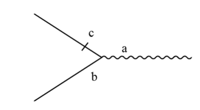
Figure 1: The triple vertex.

Strictly speaking, expression (21) should be contracted with the three transverse projectors for each of the momentum arguments of the transverse fields $\bm{v}$, $\bm{\theta}$ and $\bm{\theta}^{\prime}$ entering into the vertex. However, those projectors will effectively be restored in the diagrams, when the vertex $V_{c\,ab}$ is contracted with the transverse propagators (see expressions (22) and (23) below), so that they can be omitted in (21). The only exceptions are external vertices in 1-irreducible (amputated) diagrams, not contracted with external “legs.” For these, transverse projectors with the corresponding external momenta should be added explicitly.

The three aforementioned propagators are determined by the quadratic (free) part of the action functional. They are represented in the diagrams as slashed straight, straight and wavy lines, respectively:

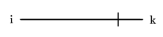
Figure 2: Diagrammatic notation for $\left\langle\theta_{i}\theta^{\prime}_{k}\right\rangle_{0}$.

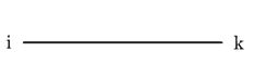
Figure 3: Diagrammatic notation for $\left\langle\theta_{i}\theta_{k}\right\rangle_{0}$.

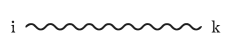
Figure 4: Diagrammatic notation for $\left\langle v_{i}v_{k}\right\rangle_{0}$.

Here the slashed end corresponds to the field $\theta^{\prime}$, the end without a slash corresponds to the field $\theta$. The line $\left\langle v_{i}v_{k}\right\rangle_{0}$ in the diagrams corresponds to the correlation function (11), and the other two propagators in the frequency-momentum representation have the forms

$$\left\langle\theta_{i}\theta^{\prime}_{k}\right\rangle_{0} = \frac{P_{ik}({\bf k})}{-i\omega+\nu_{0}({\bf k}_{\perp}^{2}+f_{0}k_{\parallel}^{2})},$$ (22)

$$\left\langle\theta_{i}\theta_{k}\right\rangle_{0} = \frac{C_{ik}({\bf k})}{\omega^{2}+\left[\nu_{0}({\bf k}_{\perp}^{2}+f_{0}k_{\parallel}^{2})\right]^{2}},$$ (23)

where $C_{ik}({\bf k})\propto P_{ik}({\bf k})$ is the Fourier transform of the function from (9).

In fact, the action functional (16) will be modified for renormalizability reasons. As a consequence, the functions (22) and (23) will acquire certain additional terms. However, it turns out that those additional terms do not contribute to the divergent parts of all the relevant diagrams, and thus can be neglected. These issues are discussed in detail in sec. IV.3, and in the following we will use for the propagators the above expressions (22) and (23).

In the time-momentum representation they take on the forms

$$\left\langle\theta_{i}(t)\theta_{k}^{\prime}(t^{\prime})\right\rangle_{0}=P_{ij}({\bf k})\cdot\Theta(t-t^{\prime})\exp\left\{-(t-t^{\prime})\epsilon_{{\bf k}}\right\},$$ (24)

$$\left\langle\theta_{i}(t)\theta_{k}(t^{\prime})\right\rangle_{0}=\left\{C_{ij}({\bf k})/2\epsilon_{{\bf k}}\right\}\,\cdot\exp\left\{-|t-t^{\prime}|\,\epsilon_{{\bf k}}\right\},$$ (25)

where $\epsilon_{{\bf k}}=\nu_{0}({\bf k}_{\perp}^{2}+f_{0}k_{\parallel}^{2})$. The propagator $\langle\theta_{i}\theta_{k}^{\prime}\rangle_{0}$ is retarded.

IV From renormalization to critical dimensions

IV.1 Canonical dimensions and UV divergences

The analysis of UV divergences is based on the analysis of canonical dimensions of the 1-irreducible Green functions. In general, dynamic models have two scales: canonical dimension of some quantity $F$ (a field or a parameter in the action functional) is completely characterized by two numbers, the frequency dimension $d_{F}^{\omega}$ and the momentum dimension $d_{F}^{k}$. They are defined such that

$$[F]\sim[T]^{-d_{F}^{\omega}}[L]^{-d_{F}^{k}},$$ (26)

where $L$ is some reference length scale and $T$ is a time scale.

In the scalar version of our strongly anisotropic model AntMal2011 , however, there are two independent length scales, related to the directions perpendicular and parallel to the vector ${\bf n}$: namely, one can introduce two independent momentum canonical dimensions $d_{F}^{\bot}$ and $d_{F}^{\parallel}$ so that $[F]\sim[T]^{-d_{F}^{\omega}}[L_{\bot}]^{-d_{F}^{\bot}}[L_{\parallel}]^{-d_{F}^{\parallel}}$, where $L_{\bot}$ and $L_{\parallel}$ are (independent) length scales in the corresponding subspaces. In the present vector model, however, we have an additional condition of the transversality of the fields $\theta$ and $\theta^{\prime}$:

$$\partial_{i}\theta_{i}=0,\quad\partial_{i}\theta^{\prime}_{i}=0,$$ (27)

which prevents the introduction of two independent scales. This issue is discussed in Appendix A in detail. In particular, this means that, in contrast to the scalar case, the constant $f_{0}$ from (14) in our case is dimensionless.

The dimensions in (26) are found from the obvious normalization conditions $d_{k}^{k}=-d_{\bf x}^{k}=1$, $d_{k}^{\omega}=-d_{\bf x}^{\omega}=0$, $d_{\omega}^{\omega}=-d_{t}^{\omega}=1$, $d_{\omega}^{k}=d_{t}^{k}=0$, and from the requirement that each term of the action functional (16) be dimensionless (with respect to the two independent dimensions separately). Based on $d_{F}^{k}$ and $d_{F}^{\omega}$, one can introduce the total canonical dimension $d_{F}=d_{F}^{k}+2d_{F}^{\omega}$ (in the free theory, $\partial_{t}\propto\partial^{2}_{\bot}\propto\partial^{2}_{\parallel}$), which plays in the theory of renormalization of dynamic models the same role as the conventional (momentum) dimension does in static problems; see, e.g., Vasiliev-Green .

Table 1: Canonical dimensions of the fields and parameters in the model (16)

$F$	$\theta^{\prime}$	$\theta$	$\bm{v}$	$M,m,\mu,\Lambda$	$\nu,\nu_{0}$	${\cal A},{\cal A}_{0}$	$f,f_{0}$	$u,u_{0}$	$\tilde{g}_{0}$, $g_{0}$	$\tilde{g}$, $g$
$d_{F}^{\omega}$	1/2	$-1/2$	1	0	1	0	0	0	0	0
$d_{F}^{k}$	$d$	0	$-1$	1	$-2$	0	0	0	$\xi$	0
$d_{F}$	$d+1$	$-1$	1	1	0	0	0	0	$\xi$	0

The canonical dimensions for the model (16) are given in Table 1, including renormalized parameters, which will be introduced a bit later. From Table 1 it follows that our model is logarithmic (the coupling constant $g_{0}\sim[L]^{-\xi}$ is dimensionless) at $\xi=0$, so that the UV divergences manifest themselves as poles in $\xi$ in the Green functions.

The total canonical dimension of an arbitrary 1-irreducible Green function $\Gamma_{N_{\Phi}}=\langle\Phi\dots\Phi\rangle_{\rm 1-ir}$ is given by the relation

$$d_{\Gamma_{N_{\Phi}}}=d+2-\sum_{\Phi}N_{\Phi}d_{\Phi}=d+2-N_{\theta^{\prime}}d_{\theta^{\prime}}-N_{\theta}d_{\theta}-N_{v}d_{v}.$$ (28)

Here $N_{\Phi}=\{N_{\theta},\,N_{\theta^{\prime}},\,N_{v}\}$ are the numbers of corresponding fields entering the function $\Gamma_{N_{\Phi}}$, and the summation over all types of the fields in (28) and analogous formulae below is always implied.

Superficial UV divergences, whose removal requires counterterms, can be present only in those functions $\Gamma_{N_{\Phi}}$ for which the “formal index of divergence” $d_{\Gamma_{N_{\Phi}}}$ is a non-negative integer. Dimensional analysis should be augmented by the following observations:

(1) In any dynamical model of type (16), 1-irreducible diagrams with $N_{\theta^{\prime}}=0$ contain closed circuits of retarded propagators (24) and therefore vanish.

(2) For any 1-irreducible Green function $N_{\theta^{\prime}}-N_{\theta}=2N_{0}$, where $N_{0}\geq 0$ is the total number of the bare propagators $\langle\theta\theta\rangle_{0}$ entering into any of its diagrams. This fact is easily checked for any given function; it is illustrated by the function with $N_{\theta^{\prime}}=N_{\theta}=1$ and $N_{0}=0$, see fig. 5. Clearly, no diagrams with $N_{0}<0$ can be drawn. Therefore, the difference $N_{\theta^{\prime}}-N_{\theta}$ is an even non-negative integer for any nonvanishing function.

(3) Using the transversality condition of the fields $\theta$ and $v$ we can move one derivative from the vertex $-\theta^{\prime}_{k}(v_{i}\partial_{i})\theta_{k}+{\cal A}_{0}\ \theta^{\prime}_{k}(\theta_{i}\partial_{i})v_{k}$ onto the field $\theta^{\prime}_{k}$. Therefore, in any 1-irreducible diagram it is always possible to move the derivative onto external “tail” $\theta^{\prime}_{k}$, which reduces the real index of divergence: $d_{\Gamma_{N_{\Phi}}}^{\prime}=d_{\Gamma_{N_{\Phi}}}-N_{\theta^{\prime}}$. The field $\theta^{\prime}_{k}$ enters into the counterterms only in the form of derivative $\partial_{i}\theta^{\prime}_{k}$.

From Table 1 and (28) we find:

$$d_{\Gamma_{N_{\Phi}}}=d+2-(d+1)N_{\theta^{\prime}}+N_{\theta}-N_{v}$$ (29)

and

$$d^{\prime}_{\Gamma_{N_{\Phi}}}\!=(d+2)(1-N_{\theta^{\prime}})+N_{\theta}-N_{v}.$$ (30)

From these expressions we conclude that, for any $d$, superficial divergences can be present only in the 1-irreducible functions of two types.

The first example is provided by the infinite family of functions $\langle\theta^{\prime}\theta\dots\theta\rangle_{\rm 1-ir}$ with $N_{\theta^{\prime}}=1$ and arbitrary $N_{\theta}$, for which $d_{\Gamma}=2$, $d_{\Gamma}^{\prime}=0$. However, all the functions with $N_{\theta}\geq N_{\theta^{\prime}}$ vanish (see above) and obviously do not require counterterms. Therefore the only nonvanishing function from this family is $\langle\theta_{\alpha}^{\prime}\theta_{\beta}\rangle_{\rm 1-ir}$.

Another possibility is $\langle\theta^{\prime}\theta\dots\theta v\dots v\rangle_{\text{1-ir}}$ with $N_{\theta^{\prime}}=1$ and arbitrary $N_{\theta}=N_{v}$, for which $d_{\Gamma}=1$, $d_{\Gamma}^{\prime}=0$. From the requirement $N_{\theta}\geq N_{\theta^{\prime}}$ it follows that the nonvanishing function of this type is $\langle\theta^{\prime}_{\alpha}\theta_{\beta}v_{\gamma}\rangle_{\text{1-ir}}$. Furthermore, from the explicit expressions (12) and (24) for the propagators it follows, that all the diagrams for that function contain closed circuits of retarded lines and therefore vanish.

Thus we are left with the only superficially divergent function $\langle\theta_{\alpha}^{\prime}\theta_{\beta}\rangle_{\rm 1-ir}$.

IV.2 Perturbation expansion for the 1-irreducible linear response function

Consider the 1-irreducible linear response function

$$\left.\Gamma_{2}^{\alpha\beta}=\langle\theta_{\alpha}^{\prime}\theta_{\beta}\rangle_{\rm 1-ir}=\frac{\delta}{\delta\theta^{\prime}_{\alpha}}\frac{\delta}{\delta\theta_{\beta}}\Gamma(\Phi)\right|_{\Phi=0},$$ (31)

where the generating function of the 1-irreducible Green functions $\Gamma(\Phi)$ (see (20)) consists of two parts,

$$\Gamma(\Phi)={\cal S}(\Phi)+\widetilde{\Gamma}(\Phi).$$ (32)

Here ${\cal S}(\Phi)$ is the action functional (16) and $\widetilde{\Gamma}(\Phi)$ is the sum of all the 1-irreducible diagrams with loops. Due to transversality of the fields in (31), the result of formal differentiation should be contracted with transverse projectors. Thus for the function $\Gamma_{2}$ one obtains

$$\Gamma_{2}^{\alpha\beta}=i\omega\cdot P_{\alpha\beta}({\bf p})-\nu_{0}{\bf p}_{\perp}^{2}\cdot P_{\alpha\beta}({\bf p})-\nu_{0}f_{0}\cdot({\bf pn})^{2}\cdot P_{\alpha\beta}({\bf p})+\Sigma_{\alpha\beta},$$ (33)

where $P_{\alpha\beta}({\bf p})=\delta_{\alpha\beta}-p_{\alpha}p_{\beta}/p^{2}$ is transverse projector and $\Sigma_{\alpha\beta}$ is the “self-energy operator,” diagrammatic representation for which is represented in the fig. 5.

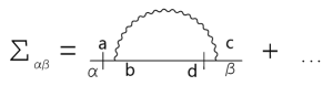
Figure 5: Diagrammatic representation for $\Sigma_{\alpha\beta}$.

Here the ellipsis stands for the 2-, 3- and other N-loop diagrams.

The typical feature of all the rapid-change models (12) with retarded bare propagator (24) is that all the skeleton multiloop diagrams entering into the self-energy operator contain closed circuits of such retarded propagators and therefore vanish. Thus the self-energy operator in (33) is exactly given by the one-loop approximation.

Let us begin the calculation of the diagram with its index structure:

$$J_{\alpha\beta}=P_{\alpha i}({\bf p})\cdot J_{ij}\cdot P_{j\beta}({\bf p}),$$ (34)

where

$$J_{ij}=V_{i\,ab}({\bf p})V_{d\,cj}({\bf p+k})P_{bd}({\bf p+k})n_{a}n_{c}.$$ (35)

Here $V_{ijk}({\bf p})$ is the triple vertex (21); the Greek letters $\alpha$, $\beta$ and the Roman letters $a$–$d$ denote the vector indices of the propagators (11), (22), (23) with the implied summation over repeated indices. Note that we need to calculate only the divergent part of the diagram, i.e., only the terms, proportional to ${\bf p}^{2}$. Some observations simplify the calculation:

(1) Because of our choice of $D_{v}$ (see (13)), namely its proportionality to $\delta(k_{\parallel})$, all the terms proportional to $k_{\parallel}$ vanish after the integration over the momentum ${\bf k}$.

(2) Both the main field $\bm{\theta}$ and the auxiliary field $\bm{\theta^{\prime}}$ are divergence-free: $\partial_{\beta}\theta_{\beta}=p_{\beta}\theta_{\beta}=0$; $\partial_{\alpha}\theta^{\prime}_{\alpha}=p_{\alpha}\theta^{\prime}_{\alpha}=0$. Thus, all the terms proportional to $p_{\alpha}$ or $p_{\beta}$ disappear after the contraction with the external fields $\bm{\theta}$ and $\bm{\theta}^{\prime}$ (see the remarks below expression (21) and the expression (34)).

This gives the following expression for the index structure of $\Sigma_{\alpha\beta}$-diagram:

$$J_{ij}=-\delta_{ij}\cdot({\bf pn})^{2}-({\cal A}_{0}-1)\cdot({\bf pn})^{2}\cdot\frac{k_{i}k_{j}}{k^{2}}+{\cal A}_{0}({\cal A}_{0}-1)\cdot({\bf pn})\cdot\frac{({\bf pk})k_{j}n_{i}}{k^{2}},$$ (36)

where we retained the terms of order ${\bf p}^{2}$.

Now we have to integrate this expression over the $d$-dimensional momentum ${\bf k}$ with the factor $1/(2\pi)^{d}\cdot D_{v}(k)$ with $D_{v}(k)$ from (13) and over the frequency $\omega$ with the factors $1/2\pi$ and $1/(-i\omega+\nu_{0}[({\bf p+k})_{\perp}^{2}+f_{0}(p+k)_{\parallel}^{2}])$:

$$\Sigma_{\alpha\beta}=\int\frac{d\omega}{2\pi}\int\frac{d{\bf k}}{(2\pi)^{d}}\frac{2\pi\,D_{0}\,\delta(k_{\parallel})\,D_{0}}{(-i\omega+\nu_{0}[({\bf p+k})_{\perp}^{2}+f_{0}(p+k)_{\parallel}^{2}])}\cdot P_{\alpha i}({\bf p})J_{ij}P_{j\beta}({\bf p})/k_{\perp}^{d-1+\xi}.$$ (37)

The integration over the frequency $\omega$ is simple due to the following interpretation of the Heaviside step function at coincided times:

$$\Theta(t-t^{\prime})={1}/{2}$$ (38)

at $t=t^{\prime}$, which is justified by the fact that the correlation function is symmetric in its arguments; cf. RG . Thus

$$\int\frac{d\omega}{2\pi}\frac{1}{(-i\omega+\nu_{0}[({\bf p+k})_{\perp}^{2}+f_{0}(p+k)_{\parallel}^{2}])}=\frac{1}{2}.$$ (39)

The integration over ${\bf k}$ with the function $\delta(k_{\parallel})$ in the integrand is performed with the aid of the relations

$$\int d{\bf k}\delta(k_{\parallel})f({\bf k})=\int d{\bf k}_{\perp}\,f({\bf k}_{\perp})=$$

$$=S_{d-1}\int_{m}^{\infty}dk_{\perp}\,k_{\perp}^{d-1}\,\left\langle f({\bf k}_{\perp})\right\rangle,$$ (40)

where $\langle\cdots\rangle$ is the averaging over the unit sphere in the $(d-1)$-dimensional space, $S_{d-1}$ is its surface area, and $k_{\perp}=|{\bf k}_{\perp}|$.

Now we need to average the two structures $k_{i}k_{j}/k^{2}$ and $({\bf pk})k_{j}/k^{2}$ from eq. (36) with the replacement $k_{i}\to k_{i}^{{\perp}}$. The first structure is orthogonal to ${\bf n}$, so the result of averaging is proportional to the transverse projector $P_{ij}({\bf n})=\delta_{ij}-n_{i}n_{j}$:

$$\left\langle\frac{k_{i}^{\perp}k_{j}^{\perp}}{k_{\perp}^{2}}\right\rangle=\frac{P_{ij}({\bf n})}{(d-1)},$$ (41)

where the coefficient is found by comparing the traces of the right and left hand sides.

Multiplying (41) to $p_{i}$, for the second structure we obtain

$$\left\langle\frac{({\bf pk}_{\perp})k^{\perp}_{j}}{k^{2}_{\perp}}\right\rangle=\frac{p_{i}P_{ij}({\bf n})}{(d-1)}\simeq-\frac{({\bf pn})n_{j}}{(d-1)}.$$ (42)

In the last relation we omitted a term proportional to $p_{j}$ because it will vanish after the contraction with the transverse projector $P_{j\beta}({\bf p})$ in expression (37).

After the angular averaging have been performed, we are left with the simple integral over the modulus $k_{\perp}$:

$$\int_{m}^{\infty}\frac{dk_{\perp}}{k_{\perp}^{1+\xi}}=\frac{m^{-\xi}}{\xi}.$$ (43)

Combining the expressions (36), (IV.2), (41) and (42) we obtain for (37) the following result:

$$\Sigma_{\alpha\beta}=-\frac{1}{2}\cdot D_{0}\cdot C_{d-1}\cdot\left[\frac{d-2+{\cal A}_{0}}{d-1}\cdot P_{\alpha\beta}({\bf p})+\frac{({\cal A}_{0}-1)^{2}}{d-1}\cdot\hat{n}_{\alpha}\hat{n}_{\beta}\right]\cdot({\bf pn})^{2}\cdot\frac{m^{-\xi}}{\xi}.$$ (44)

Here $C_{d-1}\equiv S_{d-1}/(2\pi)^{d-1}$, the amplitude $D_{0}$ was introduced in (15), and the vector $\hat{n}_{k}$, defined as

$$\hat{n}_{k}=P_{mk}({\bf p})n_{m}=n_{k}-p_{\parallel}p_{k}/p^{2},$$ (45)

is orthogonal to ${\bf p}$.

IV.3 Renormalization and bare propagators

Substituting the explicit expression (44) for the divergent part of the self-energy operator $\Sigma_{\alpha\beta}$ to the expression (33) for the 1-irreducible linear response function $\Gamma_{2}^{\alpha\beta}$ gives

$$\Gamma_{2}^{\alpha\beta}=\{i\omega\cdot-\nu_{0}{\bf p}_{\perp}^{2}-\nu_{0}f_{0}\cdot({\bf pn})^{2}\}\cdot P_{\alpha\beta}({\bf p})-D_{0}\cdot\left[\frac{d-2+{\cal A}_{0}}{2(d-1)}\cdot P_{\alpha\beta}({\bf p})+\frac{({\cal A}_{0}-1)^{2}}{2(d-1)}\cdot\hat{n}_{\alpha}\hat{n}_{\beta}\right]\cdot C_{d-1}\cdot({\bf pn})^{2}\cdot\frac{m^{-\xi}}{\xi}.$$ (46)

The renormalization constants are found from the requirement that the function (46), when expressed in new renormalized variables, be UV finite, i.e., finite at $\xi\to 0$. From the analysis of this expression it follows, however, that the pole in $\xi$ in the structure with $\hat{n}_{\alpha}\hat{n}_{\beta}$ cannot be removed by renormalization of the model parameters, because the bare part of $\Gamma_{2}^{\alpha\beta}$ does not contain analogous term. In order to ensure multiplicative renormalizability one has to add such term, with a new positive amplitude factor $u_{0}$, to the bare part:

$$\Gamma_{2}^{\alpha\beta} = \left\{i\omega-\nu_{0}{\bf p}_{\perp}^{2}-\nu_{0}f_{0}\cdot({\bf pn})^{2}\right\}\cdot P_{\alpha\beta}({\bf p})-\nu_{0}f_{0}u_{0}\cdot({\bf pn})^{2}\cdot\hat{n}_{\alpha}\hat{n}_{\beta}-$$ (47)

$$- D_{0}\cdot\left[\frac{d-2+{\cal A}_{0}}{2(d-1)}\cdot P_{\alpha\beta}({\bf p})+\frac{({\cal A}_{0}-1)^{2}}{2(d-1)}\cdot\hat{n}_{\alpha}\hat{n}_{\beta}\right]\cdot C_{d-1}\cdot({\bf pn})^{2}\cdot\frac{m^{-\xi}}{\xi}.$$

This means that the original model (16) is extended by adding the term of the form $u_{0}f_{0}\nu_{0}(n_{k}\theta_{k}^{\prime})\partial_{\parallel}^{2}\cdot(n_{k}\theta_{k})$; the interpretation of the new parameter $u_{0}$ is literally the same as for $f_{0}$ in sec. II.

Now the poles can be eliminated by multiplicative renormalization of the parameters $f_{0}$, $u_{0}$, and $g_{0}$:

$$f_{0}=fZ_{f},\ u_{0}=uZ_{u},\ g_{0}=g\mu^{\xi}Z_{g},\ Z_{g}=Z_{f}^{-1}.$$ (48)

Here $\mu$ is the “reference mass” (additional free parameter of the renormalized theory) in the minimal subtraction (MS) renormalization scheme, which we always use in what follows, $g$, $u$ and $f$ are renormalized analogs of the bare parameters $g_{0}$, $u_{0}$ and $f_{0}$, and $Z_{i}=Z_{i}(g,\xi,d)$ are the renormalization constants. Their relation in (48) results from the absence of renormalization of the contribution with $D_{v}^{-1}$ in (16), so that $D_{0}\equiv g_{0}\nu_{0}f_{0}=g\mu^{\xi}\nu f$.

No renormalization of the fields and the parameters $\nu_{0}$, ${\cal A}_{0}$ and $m_{0}=m$ is required: i.e., $Z_{\Phi}=1$ for all $\Phi$ and $Z_{\nu,m,{\cal A}}=1$. Explicit expressions for nontrivial renormalization constants will be given in the next subsection.

The renormalized action functional has the form

$${\cal S}_{R}(\Phi) = \frac{1}{2}\theta^{\prime}_{i}D_{\theta}\theta^{\prime}_{k}-\frac{1}{2}v_{i}D_{v}^{-1}v_{k}+\theta^{\prime}_{k}\left[-\partial_{t}\theta_{k}-(v_{i}\partial_{i})\theta_{k}+{\cal A}(\theta_{i}\partial_{i})v_{k}+\nu(\partial_{\perp}^{2}+fZ_{f}\cdot\partial_{\parallel}^{2})\theta_{k}\right]+$$ (49)

$$+ \nu\cdot fZ_{f}\cdot uZ_{u}\cdot(n_{k}\theta_{k}^{\prime})\partial_{\parallel}^{2}\cdot(n_{k}\theta_{k}),$$

where the function $D_{v}$ from (13) is expressed in renormalized parameters using (48).

One important question arises here. Since the original model was modified by adding a new term to the action (16), the old expressions for the propagators (22) and (23) have also changed. One may think that the whole calculation of the self-energy operator, performed in the preceding subsection, should be repeated with the new propagators. Below we show that additional terms in the modified bare propagator do not contribute to the integral (37) and revision of the final expression (47) is in fact not needed.

Let us denote the bare contribution in (47) as $-M_{\alpha\beta}$, so that

$$M_{\alpha\beta}={\cal X}\cdot P_{ij}({\bf p})+{\cal Y}\cdot\hat{n}_{i}\hat{n}_{j},$$ (50)

where

$${\cal X} = -i\omega+\nu_{0}{\bf p}_{\perp}^{2}+\nu_{0}f_{0}\cdot({\bf pn})^{2},$$ (51)

$${\cal Y} = \nu_{0}f_{0}u_{0}\cdot({\bf pn})^{2}.$$ (52)

In a conventional situation, the bare propagator $\left\langle\theta\theta^{\prime}\right\rangle_{0}$ would be given by the inverse matrix $M_{\alpha\beta}^{-1}$. Our matrix (50) has a nontrivial eigenvector with zero eigenvalue, $M_{\alpha\beta}p_{\beta}=0$, so the inverse matrix does not exist. However, the functional integration in (17) is taken over the subspace of transverse fields. Thus we do not need to invert the matrix (50) on the full momentum space, rather we need to invert it on the subspace orthogonal to the vector ${\bf p}$, where the role of the unity matrix is played by the transverse projector. Therefore the desidered “inverse” matrix

$$M^{-1}_{\alpha\beta}=x\cdot P_{ij}({\bf p})+y\cdot\hat{n}_{i}\hat{n}_{j}$$

is found from the equation

$$M_{\alpha\beta}({\bf p})\cdot M_{\beta\gamma}^{-1}({\bf p})=P_{\alpha\gamma}({\bf p}).$$ (53)

This gives

$$x=1/{\cal X};$$ (54a)

$$y=-{\cal Y}/{\cal X}({\cal X}+{\cal Y}\sin^{2}\kappa),$$ (54b)

where $\kappa$ is the angle between the vectors ${\bf n}$ and ${\bf p}$.

Thus for the propagator matrix in the modified model we obtain

$$\left\langle\theta_{\alpha}\theta^{\prime}_{\beta}\right\rangle_{0}=x\cdot P_{\alpha\beta}({\bf p})+y\cdot\hat{n}_{\alpha}\hat{n}_{\beta}$$ (55)

with the scalar coefficients $x$ and $y$ from eq. (54b). The first term coincides with the propagator (22) of the original model (16) up to the notation.

From the expressions (50) and (54b) for $y$ as a function of $\omega$ one can write

$$y=-{\cal Y}/{\cal X}({\cal X}+{\cal Y}\sin^{2}\kappa)\propto\frac{({\bf pn})^{2}}{(-i\omega+\eta_{1})(-i\omega+\eta_{2})}$$ (56)

with certain $\eta_{1}$, $\eta_{2}>0$ that depend only on the momentum. The both poles in $\omega$ in expression (56) lie in the same lower half of the complex plane. Thus the integral over $\omega$ of this expression vanishes identically. It is important here that the integral is convergent by power counting, and the ambiguity similar to that in the integral (39) is absent here.

This means that the new term in the propagator does not contribute to the integral (37) and the expression (47) remains valid in the modified model. Of course, the contribution with $y$ shoud be taken into account in calculations of the other Green functions.

Some additional remarks about our scheme of derivation of the propagators and its justification on the example of a simple model are given in Appendix B.

IV.4 RG equations and fixed points

Now let us introduce the $\beta$ functions and the anomalous dimensions $\gamma$ – important RG functions, which determine the asymptotic behavior of the various Green functions. The basic RG equation for a multiplicatively renormalizable quantity (correlation function, composite operator, etc.) is obtained by operating with $\widetilde{{\cal D}}_{\mu}$ on the relation $F=Z_{F}F_{R}$, where $\widetilde{\cal D}_{\mu}$ denotes the differential operation $\mu\partial_{\mu}$ for fixed set of bare parameters $e_{0}$ $=$ $\left\{g_{0},\nu_{0},f_{0},u_{0},{\cal A}_{0}\right\}$. The resulting RG equation has the form

$$\bigl{[}{\cal D}_{RG}+\gamma_{F}\bigr{]}F_{R}=0,$$ (57)

where $\gamma_{F}$ is the anomalous dimension of $F$ and ${\cal D}_{RG}={\cal D}_{\mu}+\beta\partial_{g}-\gamma_{f}{\cal D}_{f}-\gamma_{u}{\cal D}_{u}$. Here and below ${\cal D}_{x}\equiv x\partial_{x}$ for any variable $x$, and the RG functions are defined as

$$\beta_{g}\equiv\widetilde{\cal D}_{\mu}g=g\cdot[-\xi-\gamma_{g}(g)],$$ (58a)

$$\beta_{u}\equiv\widetilde{\cal D}_{\mu}u=-u\gamma_{u}(g,u),$$ (58b)

$$\gamma_{F}\equiv\widetilde{\cal D}_{\mu}\ln Z_{F}=\beta_{g}\partial_{g}\ln Z_{F}\quad{\rm for\ any\ }Z_{F}.$$ (58c)

The relations between $\beta$ and $\gamma$ in (58a) and (58b) result from their definitions along with the second and third relations in (48).

As already stated, the constants $Z$ are found from the requirement of UV finiteness of the expression (47) by means of the relations $D_{0}g_{0}f_{0}\nu_{0}=gf\nu\mu^{\xi}$ and (48). Thus we readily obtain the renormalization constant $Z_{f}$ ($f_{0}=f\cdot Z_{f}$) and the anomalous dimension $\gamma_{f}$ for the parameter $f_{0}$ that splits the Laplace operator:

$$Z_{f}=1-\frac{d-2+{\cal A}}{2(d-1)}\cdot\frac{g}{\xi}+O(g^{2}),$$ (59)

$$\gamma_{f}=\frac{d-2+{\cal A}}{2(d-1)}\cdot g,$$ (60)

where we passed to the new coupling constant $g\equiv\tilde{g}\cdot C_{d-1}$ with $C_{d-1}$ from (44). Then we have to renormalize the constant $u_{0}$ such that the expression

$$g_{0}f_{0}u_{0}\cdot\left[1+\frac{({\cal A}-1)^{2}}{2(d-1)}\cdot\frac{1}{u_{0}}\cdot\frac{m^{-\xi}}{\xi}\right]\cdot n_{\alpha}n_{\beta}\cdot({\bf pn})^{2}$$ (61)

be UV finite to the first order in $g$. Therefore,

$$Z_{u}\cdot Z_{f}=1-\frac{({\cal A}-1)^{2}}{2(d-1)}\cdot\frac{g}{u}\cdot\frac{1}{\xi}+O(g^{2})$$ (62)

and

$$\gamma_{u}+\gamma_{f}=\frac{({\cal A}-1)^{2}}{2(d-1)}\cdot\frac{1}{u}\cdot g$$ (63)

with the constant $\gamma_{f}$ from 60. Furthermore, from the last relation in (48) it follows that for the coupling constant $g$

$$\gamma_{g}=-\gamma_{f}=-\frac{d-2+{\cal A}}{2(d-1)}\cdot g.$$ (64)

We stress that all the above expressions for the anomalous dimensions $\gamma_{F}$ are exact, being derived from the exact expression (47).

One of the basic RG statements is that the IR asymptotic behavior of the model is governed by the IR attractive fixed point $g^{*}$, $u^{*}$, defined by the relations

$$\beta_{u}=0,\ \ \partial_{u}\beta_{u}>0;\ \ \beta_{g}=0,\ \ \partial_{g}\beta_{g}>0.$$ (65)

For the coupling constant $g$ these equations along with (64) give

$$\beta_{g}=g(-\xi+\gamma_{f})=0,$$ (66)

and the fixed point is

$$g^{*}=\frac{2(d-1)}{d-2+{\cal A}}\cdot\xi,\ \ \partial_{g}\beta_{g}(g^{*})=\xi>0.$$ (67)

The $\beta$-function and the fixed point for second parameter $u$ are

$$\beta_{u}=-u\gamma_{u}=g\cdot\frac{1}{2(d-1)}\left[(d-2+{\cal A})\cdot u-({\cal A}-1)^{2}\right],$$ (68)

so that

$$u^{*}=\frac{({\cal A}-1)^{2}}{d-2+{\cal A}},\ \ \partial_{u}\beta_{u}(u^{*})=\frac{d-2+{\cal A}}{2(d-1)}\cdot g^{*}.$$ (69)

Therefore, the system possesses an IR fixed point $u^{*},g^{*}$ only if $g^{*}>0$, i.e.,

$$d-2+{\cal A}>0.$$ (70)

This fact implies that the correlation functions of the model (16) in the IR region ($\mu r\simeq\Lambda r\gg 1$, $Mr\sim 1$) exhibit scaling behavior (as we will see below, up to logarithmic factors).

The corresponding critical dimensions $\Delta[F]\equiv\Delta_{F}$ for all basic fields and parameters can be calculated exactly; see the next subsection.

IV.5 Critical dimensions

In the leading order of the IR asymptotic behavior the Green functions satisfy the RG equation with the substitution $g\to g_{*}$, $u\to u_{*}$, which gives

$$\left[{\cal D}_{\mu}-\gamma_{f}^{*}{\cal D}_{f}-\gamma_{u}^{*}{\cal D}_{u}+\gamma_{G}^{*}\right]\,G^{R}(e,\mu,\dots)=0.$$ (71)

Canonical scale invariance is expressed by the relations:

$$\left[\sum_{\alpha}d_{\alpha}^{k}{\cal D}_{\alpha}-d_{G}^{k}\right]G^{R}=0,\quad\left[\sum_{\alpha}d_{\alpha}^{\omega}{\cal D}_{\alpha}-d_{G}^{\omega}\right]G^{R}=0,$$ (72)

where $\alpha\equiv\{t,{\bf x},\mu,\nu,m,M,u,f,{\cal A},g\}$ is the set of all arguments of $G^{R}$ ($t,{\bf x}$ is the set of all times and coordinates), and $d^{k}$ and $d^{\omega}$ are the canonical dimensions of $G^{R}$ and $\alpha$. Substituting the needed dimensions from Table 1 into (72), we obtain:

$$\left[{\cal D}_{\mu}+{\cal D}_{m}+{\cal D}_{M}-2{\cal D}_{\nu}-{\cal D}_{\bf x}-d_{G}^{k}\right]G^{R}=0,$$ (73a)

$$\left[{\cal D}_{\nu}-{\cal D}_{t}-d_{G}^{\omega}\right]G^{R}=0.$$ (73b)

The equations of the type (71) and (73) describe the scaling behavior of the function $G^{R}$ upon the dilation of a part of its parameters. A parameter is dilated if the corresponding derivative enters the equation, otherwise it is kept fixed. We are interested in the IR scaling behavior, in which all the IR relevant parameters (coordinates ${\bf x}$, times $t$ and integral scales $M$ and $m$) are dilated, while the irrelevant parameters, related to the UV scale (diffusivity coefficient $\nu$ and the renormalization mass $\mu$) are fixed. Thus we combine the equations (71) and (73) such that the derivatives with respect to the IR irrelevant parameters $\mu$ and $\nu$ be eliminated, and obtain the desired equation of critical IR scaling for the model:

$$\left[-{\cal D}_{\bf x}+\Delta_{t}{\cal D}_{t}+\Delta_{m}{\cal D}_{m}+\Delta_{M}{\cal D}_{M}+\right.$$

$$\left.+\Delta_{f}{\cal D}_{f}+\Delta_{u}{\cal D}_{u}-\Delta_{G}\right]G^{R}=0,$$ (74)

where

$$\Delta_{t}=-\Delta_{\omega}=-2,\quad\Delta_{m}=\Delta_{M}=1,$$

$$\Delta_{f}=\gamma_{f}^{*},\quad\Delta_{u}=\gamma_{u}^{*}$$ (75)

and

$$\Delta[G]\equiv\Delta_{G}=d_{G}^{k}+2d_{G}^{\omega}+\gamma_{G}^{*}$$ (76)

are the corresponding critical dimensions.

In particular, for any correlation function $G^{R}=\langle\Phi\dots\Phi\rangle$ of the fields $\Phi$ we have $\Delta_{G}=N_{\Phi}\Delta_{\Phi}$, with the summation over all fields $\Phi$ entering into $G^{R}$, namely

$$\Delta_{G}=\sum_{\Phi}N_{\Phi}d_{\Phi}=N_{\theta^{\prime}}d_{\theta^{\prime}}+N_{\theta}d_{\theta}+N_{v}d_{v}.$$ (77)

Since in the model (16) the fields themselves are not renormalized (i.e., $\gamma_{\Phi}=0$ for all $\Phi$, see sec. IV.3), using (76) we conclude, that the critical dimensions of the fields $\Phi=\left\{\bm{v},{\bm{\theta}},{\bm{\theta}^{\prime}}\right\}$ are the same as their canonical dimensions, presented in the Table 1. Namely,

$$\Delta_{\bm{v}}=1,\quad\Delta_{\theta}=-1,\quad\Delta_{\theta^{\prime}}=d+1.$$ (78)

It is the specific feature of this model, which distinguishes it from both the isotropic Kraichnan’s vector model AntGul2012 (in which $\gamma_{\nu}\neq 0$) and anisotropic Kraichnan’s scalar model AntMal2011 (in which the Laplacian splitting parameter $f$ is not dimensionless).

V Renormalization and critical dimensions of composite operators

V.1 General scheme

In the following, the central role will be played by composite fields (“operators”) built solely of the basic fields $\theta$:

$$F_{Np}=(\theta_{i}\theta_{i})^{p}\ (n_{s}\theta_{s})^{2m},$$ (79)

where $N=2(p+m)$ is the total number of fields $\theta$, entering the operator.

The total canonical dimension of arbitrary 1-irreducible Green function $\Gamma=\langle F\Phi\dots\Phi\rangle_{1-ir}$ that includes one composite operator $F$ and arbitrary number of primary fields $\Phi$ is given by the relation

$$d_{\Gamma}=d_{F}-\sum_{\phi}N_{\Phi}d_{\Phi}=-(N-N_{\theta})-(d+1)N_{\theta^{\prime}}-N_{v},$$ (80)

where $d_{F}$ is the canonical dimension of the operator $F$; see, e.g., sec. 3.24 in the book Vasiliev-Green .

Superficial UV divergences, whose removal requires counterterms, can be present only in those functions $\Gamma$ for which the index of divergence $d_{\Gamma_{N_{\Phi}}}$ is a non-negative integer. For the operators of the form (79) one has $d_{F}=-N$; see Table 1. Due to the linearity of our model, the number of the fields $\theta$ in the function $\Gamma$ cannot exceed their number in the operator $F$; cf. item (2) in sec. IV.1. In the case at hand

$$N_{\theta}\leq N.$$ (81)

From the expression (80) along with the condition (81) it follows that for any dimension of the space $d$ superficial divergences can be present only in the 1-irreducible functions of the type $\bigl{\langle}F_{Np}(x)\theta(x_{1})\dots\theta(x_{N})\bigr{\rangle}_{\rm 1-ir}$ with $N_{\theta}=N$, $N_{v}=N_{\theta^{\prime}}=0$, for which $d_{\Gamma_{F}}=0$. This means, in particular, that all those diagrams diverge logarithmically and we can calculate them with all external frequencies and momenta set equal to zero. This also means that the operator counterterms to a certain $F_{Np}$ include only operators of the form (79) with the same value of $N$.

We conclude that the operators (79) can mix in renormalization only within the closed set with the same $N$; let us denote it as $F\equiv\{F_{Np}\}$. The renormalization matrix $\hat{Z}_{F}\equiv\{Z_{Np,Np^{\prime}}\}$ for this set, given by the relation

$$F_{Np}=\sum_{p^{\prime}}Z_{Np,Np^{\prime}}F_{Np^{\prime}}^{R},$$ (82)

is determined by the requirement that the 1-irreducible correlation function

$$\bigl{\langle}F_{Np}^{R}(x)\theta(x_{1})\dots\theta(x_{N})\bigr{\rangle}_{\rm 1-ir}=$$

$$=\sum_{p^{\prime}}Z_{Np,\,Np^{\prime}}^{-1}\bigl{\langle}F_{Np^{\prime}}(x)\theta(x_{1})\dots\theta(x_{N})\bigr{\rangle}_{\rm 1-ir}\equiv\sum_{p^{\prime}}Z_{Np,\,Np^{\prime}}^{-1}\Gamma_{Np^{\prime}}(x;x_{1},\dots,x_{N})$$ (83)

be UV finite in renormalized theory, that is, it has no poles in $\xi$ when expressed in renormalized variables (48). This is equivalent to the UV finiteness of the sum $\sum_{p^{\prime}}Z_{Np,\,Np^{\prime}}^{-1}\Gamma_{Np^{\prime}}(x;\theta)$, in which

$$\Gamma_{Np^{\prime}}(x;\theta)=\frac{1}{N!}\,\int dx_{1}\dots\int dx_{N}\,\Gamma_{Np^{\prime}}(x;x_{1},\dots,x_{N})\times$$

$$\times\theta(x_{1})\dots\theta(x_{N})$$ (84)

is a functional of the field $\theta(x)$.

The contribution of a specific diagram into the functional $\Gamma_{Np^{\prime}}$ in (84) for any composite operator $F_{Np^{\prime}}$ is represented in the form

$$\Gamma_{Np^{\prime}}=V_{\alpha\beta\dots}\,I^{ab\dots}_{\alpha\beta\dots}\,\theta_{a}\theta_{b}\dots,$$ (85)

where $V_{\alpha\beta\dots}$ is the vertex factor, $I^{ab\dots}_{\alpha\beta\dots}$ is the “internal block” of the diagram with free indices, and the product $\theta_{a}\theta_{b}\dots$ corresponds to external tails.

According to the general rules of the universal diagrammatic technique (see, e.g., Vasiliev-Green ), for any composite operator $F(x)$ built of the fields $\theta$, the vertex $V_{\alpha\beta\dots}$ in (85) with $k\geq 0$ attached lines corresponds to the vertex factor

$$V^{k}_{Np}(x;\,x_{1},\dots,x_{k})\equiv\delta^{k}F_{Np}(x)/{\delta\theta(x_{1})\dots\delta\theta(x_{k})}.$$ (86)

The arguments $x_{1}\dots x_{k}$ of the quantity (86) are contracted with the arguments of the upper ends of the tails $\theta\theta^{\prime}$ attached to the vertex.

V.2 One-loop diagram

Now let us turn to calculate the internal block $I^{ab\dots}_{\alpha\beta\dots}$ in the notation (85), namely the diagrams themselves. The one-loop diagram is represented in fig. (6).

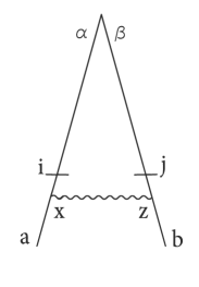
Figure 6: The one-loop contribution to the generating functional.

We recall that all the external frequencies and momenta are set to zero. Then the index structure of this diagram is

$$Y^{ab}_{\alpha\beta}=V_{xai}({\bf k})\ V_{zjb}({\bf-k})\cdot P_{\alpha i}({\bf k})\ P_{\beta j}({\bf k})\cdot n_{x}n_{z}=$$

$$=-{\cal A}^{2}\cdot n_{x}P_{x\alpha}({\bf k})\cdot n_{z}P_{z\beta}({\bf k})\cdot k_{a}k_{b},$$ (87)

where the letters $i,j,x$ and $z$ denote internal indices of the diagram itself. Then we have to integrate $Y^{ab}_{\alpha\beta}$ over the frequency and momentum with the factors like (12) and (22), namely

$$I^{ab}_{\alpha\beta}=\int\frac{d{\bf k}}{(2\pi)^{d}}\cdot\frac{1}{-i\omega+\nu{\bf k}_{\perp}^{2}+\nu fk_{\parallel}^{2}}\cdot\frac{1}{i\omega+\nu{\bf k}_{\perp}^{2}+\nu fk_{\parallel}^{2}}\times$$

$$\times D_{0}\cdot\frac{\delta(k_{\parallel})}{k_{\perp}^{d-1+\xi}}\cdot Y^{ab}_{\alpha\beta}.$$ (88)

Due to the presence of the factor $\delta(k_{\parallel})$ in the above expression, the additional part (56) in the propagator $\langle\theta\theta^{\prime}\rangle_{0}$ gives no contribution in all integrals corresponding to the diagrams, and like for the self-energy function, we can perform all the calculations with the original propagators (22) and (23).

Using (41) for averaging over the angles, we arrive at the following result:

$$I^{ab}_{\alpha\beta}=\frac{{\cal A}^{2}}{2\nu}\cdot D_{0}\cdot\int\frac{d{\bf k}_{\perp}}{(2\pi)^{d}}\ \frac{1}{k_{\perp}^{d-1+\xi}}\cdot\frac{k_{a}^{\perp}k_{b}^{\perp}}{k^{2}_{\perp}}\cdot n_{\alpha}n_{\beta}=$$

$$=\frac{{\cal A}^{2}\cdot f}{2\ (d-1)}\cdot P_{ab}({\bf n})\cdot n_{\alpha}n_{\beta}\cdot\ g\cdot\frac{m^{-\xi}}{\xi}.$$ (89)

V.3 Multiloop diagrams

Any multiloop diagram contains a part with the structure, represented in fig. (7).

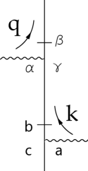
Figure 7: Fragment of arbitrary multiloop diagram.

Since we may calculate all the diagrams at external momenta set equal to zero, the integral, corresponding to the divergent part of the diagram, contains as a factor the following expression:

$$I_{0}=\delta(k_{\parallel})\delta(q_{\parallel})n_{a}V_{bac}({\bf k})n_{\alpha}V_{\beta\alpha\gamma}({\bf k+q})P_{\gamma b}({\bf k}),$$ (90)

where $V$ is the vertex (21), and the $\delta$-functions appear from velocity correlator (11). Since $I_{0}$ is proportional to the sum of $k_{\parallel}$ and $q_{\parallel}$ with some coefficients, after integration with the $\delta$-functions all these diagrams become equal to zero.

There are also multiloop diagrams of the “sand clock” type, represented by products of simpler diagrams. They contain only higher-order poles in $\xi$ and, in the MS scheme, do not contribute to the anomalous dimensions.

Therefore (and it is another special feature of this model) the one-loop approximation (89) gives us the exact answer.

V.4 Renormalization matrix and anomalous dimensions

Combining expressions (85), (86) and the exact answer (89) for the diagram we obtain for the functional $\Gamma_{Np}$ from (84)

$$\Gamma_{Np} \propto \frac{\delta^{2}}{\delta\theta_{\alpha}\cdot\delta\theta_{\beta}}\left[F_{Np}\right]\cdot n_{\alpha}n_{\beta}\cdot P_{ab}({\bf n})\ \theta_{a}\theta_{b}=$$ (91)

$$= 2m(2m-1)\cdot F_{N\,p+1}\ +\ (2p+8pm-2m(2m-1))\cdot F_{N\,p}\ +$$

$$+ (4p(p-1)-2p-8pm)\cdot F_{N\,p-1}\ -\ 4p(p-1)\cdot F_{N\,p-2},$$

up to an overall scalar factor.

Expression (91) shows that the operators $F_{Np}$ indeed mix in renormalization: the UV finite renormalized operator $F^{R}$ has the form $F^{R}=F+$ counterterms, where the contribution of the counterterms is a linear combination of $F$ itself and other unrenormalized operators with the same total number $N$ of the fields, which are said to “admix” to $F$ in renormalization.

Let $F\equiv\{F_{p}\}$ be a closed set of operators (79) with a certain fixed value of $N$ (which we will omit below for brevity) and different values of $p$, which mix only to each other in renormalization. The renormalization matrix $\hat{Z}_{F}\equiv\{Z_{p,p^{\prime}}\}$ and the matrix of anomalous dimensions $\hat{\gamma}_{F}\equiv\{\gamma_{p,p^{\prime}}\}$ for this set are given by

$$F_{p}=\sum_{p^{\prime}}Z_{p,p^{\prime}}F_{p^{\prime}}^{R},\quad\hat{\gamma}_{F}=\hat{Z}_{F}^{-1}{\cal D}_{\mu}\hat{Z}_{F}.$$ (92)

The scale invariance (72) and the RG equation (57) for the operator $F_{p}$ give us the corresponding matrix of critical dimensions $\Delta_{F}\equiv\{\Delta_{p,p^{\prime}}\}$ in the form similar to the expression (76), in which $d_{F}^{k}$, $d_{F}^{\omega}$ and $d_{F}$ are understood as the diagonal matrices of canonical dimensions of the operators in question (with the diagonal elements equal to sums of corresponding dimensions of all fields and derivatives constituting $F$) and $\hat{\gamma}^{*}=\hat{\gamma}(g^{*},u^{*})$ is the matrix (92) at the fixed point.

In this notation and in the MS scheme the renormalization matrix $\hat{Z}$ has the form

$$\hat{Z}=\hat{I}+\hat{A},$$ (93)

where $\hat{I}$ is the unity matrix and the elements of the matrix $\hat{A}$ have the form

$$A_{pp^{\prime}}=a_{pp^{\prime}}\cdot\frac{g}{\xi}.$$ (94)

To solve the RG equation we have to use the eigenvalue decomposition of the matrix $\hat{\gamma}$, therefore the critical dimensions of the set $F\equiv\{F_{p}\}$ are given by the eigenvalues of the matrix $\Delta_{pp^{\prime}}$. In fact this means, that we change the set of operators $\left\{F^{R}\right\}$ to the set of “basis” operators $\left\{\widetilde{F}^{R}\right\}$ that possess definite critical dimensions and have the form

$$F^{R}_{p}=U_{pp^{\prime}}\widetilde{F}^{R}_{p^{\prime}},$$ (95)

where the matrix $U_{pp^{\prime}}$ is such that $\widetilde{\Delta}_{F}=U_{F}^{-1}\Delta_{F}U_{F}$ is diagonal (or has the Jordan form).

As the renormalization matrix $\hat{Z}$ has the form (93), the matrix of anomalous dimensions $\hat{\gamma}$ has the form

$$\gamma_{pp^{\prime}}=-a_{pp^{\prime}}\cdot g$$ (96)

with the coefficients $a_{pp^{\prime}}$ from (94). Combining (91)–(96) and taking into account the scalar factor, not written in (91), but presented in (89), together with the fact, that the symmetrical coefficient for this one-loop diagram is $1/2$, one can obtain the following for the matrix of anomalous dimensions $\hat{\gamma}$:

$$\gamma_{p,\,p^{\prime}+1} = -\frac{{\cal A}^{2}\cdot f}{4(d-1)}\cdot 2m(2m-1)\cdot g;$$

$$\gamma_{p,\,p^{\prime}} = -\frac{{\cal A}^{2}\cdot f}{4(d-1)}\cdot(2p+8pm-2m(2m-1))\cdot g;$$

$$\gamma_{p,\,p^{\prime}-1} = -\frac{{\cal A}^{2}\cdot f}{4(d-1)}\cdot(4p(p-1)-2p-8pm)\cdot g;$$

$$\gamma_{p,\,p^{\prime}-2} = -\frac{{\cal A}^{2}\cdot f}{4(d-1)}\cdot(-4p(p-1))\cdot g.$$ (97)

Substituting the value of the fixed point $g^{*}=\frac{2(d-1)}{d-2+{\cal A}}\cdot\xi$ (see (67)) gives

$$\gamma_{p,\,p^{\prime}+1}^{*} = -\frac{{\cal A}^{2}\cdot f}{2(d-2+{\cal A})}\cdot 2m(2m-1)\cdot\xi;$$

$$\gamma_{p,\,p^{\prime}}^{*} = -\frac{{\cal A}^{2}\cdot f}{2(d-2+{\cal A})}\cdot(2p+8pm-2m(2m-1))\cdot\xi;$$

$$\gamma_{p,\,p^{\prime}-1}^{*} = -\frac{{\cal A}^{2}\cdot f}{2(d-2+{\cal A})}\cdot(4p(p-1)-2p-8pm)\cdot\xi;$$

$$\gamma_{p,\,p^{\prime}-2}^{*} = -\frac{{\cal A}^{2}\cdot f}{2(d-2+{\cal A})}\cdot(-4p(p-1))\cdot\xi.$$ (98)

Therefore the critical dimensions matrix for the set $F_{p}$ has the form

$$\Delta_{p,\,p^{\prime}}=-2(p+m)\cdot\delta_{pp^{\prime}}+\hat{\gamma}^{*}_{p,\,p^{\prime}},$$ (99)

where $-2(p+m)$ is its canonical dimension, $\delta_{pp^{\prime}}$ is Kronecker’s $\delta$ symbol and $\hat{\gamma}^{*}_{p,p^{\prime}}$ is the value of anomalous dimension matrix at the fixed point.

V.5 Critical dimension matrix and its eigenvalue decomposition

Let us find the eigenvalues of the critical dimensions matrix $\Delta_{Np,Np^{\prime}}$ (from now on, we restore the index $N$ in the notation for the operators and related matrices). As a consequence of (V.4), it is a four-diagonal matrix for any $N$; moreover it has one line under the main diagonal and two lines above the main diagonal. Therefore the inversion of the matrix and its eigenvalue decomposition appear nontrivial tasks.

According to (91), the closed set $F\equiv\{F_{Np}\}$ of operators, which mix only with each other in renormalization, consists only of operators with the same total quantity of fields $\theta$, i.e., with the same number $N$. So, let us define the vector ${\bf F}$ as

$${\bf F}=\begin{pmatrix}(\theta_{i}\theta_{i})^{N}\\ (\theta_{i}\theta_{i})^{N-2}\cdot(n_{s}\theta_{s})^{2}\\ \vdots\\ (n_{s}\theta_{s})^{N}\end{pmatrix}.$$ (100)

Therefore the relation between the set of unrenormalized operators $\left\{F\right\}$ and the set of renormalized operators $\left\{F^{R}\right\}$, namely $F_{i}=Z_{ik}F_{k}^{R}$, takes on the form

$$\begin{pmatrix}(\theta_{i}\theta_{i})^{N}\\ (\theta_{i}\theta_{i})^{N-2}\cdot(n_{s}\theta_{s})^{2}\\ (\theta_{i}\theta_{i})^{N-4}\cdot(n_{s}\theta_{s})^{4}\\ \vdots\\ \vdots\\ (\theta_{i}\theta_{i})^{2}\cdot(n_{s}\theta_{s})^{N-2}\\ (n_{s}\theta_{s})^{N}\end{pmatrix}=\begin{pmatrix}a_{11}&a_{12}&a_{13}&0&\dots&0\\ a_{21}&a_{22}&a_{23}&a_{24}&&\vdots\\ 0&a_{32}&a_{33}&a_{34}&\ddots&0\\ \vdots&0&a_{43}&\ddots&\ddots&a_{n-2n}\\ \vdots&&&\ddots&\ddots&a_{n-1n}\\ 0&\dots&\dots&0&a_{nn-1}&a_{nn}\end{pmatrix}\cdot\begin{pmatrix}\left\{(\theta_{i}\theta_{i})^{N}\right\}^{R}\\ \left\{(\theta_{i}\theta_{i})^{N-2}\cdot(n_{s}\theta_{s})^{2}\right\}^{R}\\ \left\{(\theta_{i}\theta_{i})^{N-4}\cdot(n_{s}\theta_{s})^{4}\right\}^{R}\\ \vdots\\ \vdots\\ \left\{(\theta_{i}\theta_{i})^{2}\cdot(n_{s}\theta_{s})^{N-2}\right\}^{R}\\ \left\{(n_{s}\theta_{s})^{N}\right\}^{R}\end{pmatrix}.$$ (101)

It is important that in this notation the row of the matrix $\hat{Z}$ corresponds to the original unrenormalized operator, and that the power $p$ of the operator $F_{Np}$ decreases from left to right.

Let us denote the common factor in (V.4) as $y$, i.e.,

$$y=-\frac{{\cal A}^{2}\cdot f}{2(d-2+{\cal A})}\cdot\xi,$$ (102)

and construct from (V.4), (99) and (101) the matrix of critical dimensions for several sets of operators. For example, for the set with $N=2$ we have

$$N=2:\ \ \ \Delta_{Np,Np^{\prime}}=\begin{pmatrix}-2+2y&-2y\\ 2y&-2-2y\end{pmatrix},$$ (103)

and the eigenvalues are $\lambda=\left\{-2;-2\right\}$; for the set with $N=8$ we have

$$N=8:\ \ \ \Delta_{Np,Np^{\prime}}=$$

$$=\begin{pmatrix}-8+8y&40y&-48y&0&0\\ 2y&-8+28y&-6y&-24y&0\\ 0&12y&-8+24y&-28y&-8y\\ 0&0&30y&-8-4y&-26y\\ 0&0&0&56y&-8-56y\end{pmatrix},$$ (104)

and the eigenvalues are $\lambda=\left\{-8;-8;-8;-8;-8\right\}$; and so on. This fact remains true for ${\it any}$ set of operators with arbitrary number $N$. This statement is strictly proven in Appendix C.

In other words, for any $N$, the matrix of anomalous dimensions (V.4) is nilpotent, and the matrix of critical dimensions (99) is degenerate with all the eigenvalues equal to $N$:

$$\lambda_{1}=\ \dots\ =\lambda_{N/2+1}=-2(p+m)=-N.$$ (105)

Therefore the matrix of critical dimensions (99) is not diagonalizable, but can be brought to a Jordan form, i.e., $\Delta_{F}=U_{F}\widetilde{\Delta}_{F}U_{F}^{-1}$, and for the matrix $\widetilde{\Delta}_{F}$ we can write

$$\widetilde{\Delta}_{F}=\begin{pmatrix}-2(p+m)&1&0&\dots&0\\ 0&-2(p+m)&1&&\vdots\\ \vdots&0&\ddots&\ddots&0\\ \vdots&&&\ddots&1\\ 0&\dots&&0&-2(p+m)\end{pmatrix}.$$ (106)

The matrix $U_{F}$, which brings it to the Jordan form, is triangular, namely

$$U_{F}=\begin{pmatrix}u_{11}&u_{12}&u_{13}&\dots&\dots&u_{1n}\\ u_{21}&u_{22}&\dots&\dots&u_{2n-1}&0\\ u_{31}&\vdots&&~{}\reflectbox{$\ddots$}&&\vdots\\ \vdots&\vdots&~{}\reflectbox{$\ddots$}&\ &&\vdots\\ u_{n-1\ 1}&u_{n-1\ 2}&&&&\vdots\\ u_{n1}&0&\dots&\dots&\dots&0\end{pmatrix},$$ (107)

with the elements $u_{ik}\neq 0$ for all $i$, $k$ (for detailed discussion see Appendix C).

V.6 Asymptotic behavior of the mean value of operator $F_{Np}$

The objects of interest are, in particular, the equal-time correlation functions $G=\left\langle F_{1}F_{2}\right\rangle$. In using the operator product expansion (OPE), the mean values of the operators $\left\langle F^{R}\right\rangle$ will appear in the right hand side (see below). Therefore now it is useful to understand the asymptotic behavior of the quantities $\left\langle F^{R}\right\rangle$ themselves.

From the dimensionality considerations it follows that

$$\left\langle{\bf\widetilde{F}}^{R}\right\rangle\propto\nu^{d^{\omega}_{F}}\mu^{d_{F}}\cdot\widehat{\Phi}\left(\frac{M}{\mu},f\right)\cdot\widehat{{\bf C}}_{0}.$$ (108)

If an operator $F$ itself is multiplicatively renormalizable, in the IR-region it satisfies the differential equation (74)–(75), which describes the IR scaling behavior. The solution of this equation (the mean value does not depend on the time $t$ and coordinates ${\bf x}$) gives us the asymptotic form:

$$\left\langle{\bf\widetilde{F}}^{R}\right\rangle\propto M^{\widetilde{\Delta}_{F}}\cdot\Phi\left(\frac{f}{M^{\gamma_{f}^{*}}}\right)\cdot{\bf C}_{0}.$$ (109)

This along with the dimensionality representation (108) gives

$$\left\langle{\bf\widetilde{F}}^{R}\right\rangle\propto\nu^{d^{\omega}_{F}}\mu^{d_{F}}\cdot\left(M/\mu\right)^{\widetilde{\Delta}_{F}}\cdot\Phi\left(\frac{f}{(M/\mu)^{\xi}}\right)\cdot{\bf C}_{0},$$ (110)

where $\Phi$ is some unknown function of the dimensionless argument, $\gamma_{f}^{*}=\xi$ (see equations (60) and (67)), ${\bf\widetilde{F}}^{R}$ is a vector built from the “basis” operators (95) that possess definite critical dimensions, ${\bf C}_{0}$ is some constant vector (“initial data”), $\mu$ is the renormalization mass, $\nu$ is the viscosity coefficient, $M$ is the parameter, related to the external turbulence scale connected to the stirring (see expression (9)) and $\widetilde{\Delta}_{F}$ is the matrix of critical dimensions from (106).

Since the matrix $\widetilde{\Delta}_{F}$ in (110) has a Jordan form with the only degenerate eigenvalue $\lambda_{0}=-2(p+m)$, then the value of a certain scalar function ${\cal F}$ with the matrix argument $\widetilde{\Delta}_{F}$ is given by the matrix ${\cal F}\left(\widetilde{\Delta}_{F}\right)$:

$${\cal F}\left(\widetilde{\Delta}_{F}\right)=\begin{pmatrix}{\cal F}\left(\lambda_{0}\right)&\frac{{\cal F}^{\prime}\left(\lambda_{0}\right)}{1!}&\dots&\frac{{\cal F}^{(n-1)}\left(\lambda_{0}\right)}{(n-1)!}\\ 0&{\cal F}\left(\lambda_{0}\right)&&\vdots\\ \vdots&&\ddots&\frac{{\cal F}^{\prime}\left(\lambda_{0}\right)}{1!}\\ 0&\dots&0&{\cal F}\left(\lambda_{0}\right)\end{pmatrix}.$$ (111)

If the function ${\cal F}$ is chosen as $(M/\mu)^{\widetilde{\Delta}_{F}}$, the logarithms $\ln(M/\mu)$ will appear in the sought-for asymptotic expression:

$$(M/\mu)^{\widetilde{\Delta}_{F}}=\begin{pmatrix}(M/\mu)^{\lambda}&(M/\mu)^{\lambda}\cdot\ln(M/\mu)&\dots&\frac{(M/\mu)^{\lambda}\cdot(\ln(M/\mu))^{n-1}}{(n-1)!}\\ 0&(M/\mu)^{\lambda}&&\vdots\\ \vdots&&\ddots&(M/\mu)^{\lambda}\cdot\ln(M/\mu)\\ 0&\dots&0&(M/\mu)^{\lambda}\end{pmatrix}.$$ (112)

Therefore, after the convolution with the initial-data vector ${\bf C}_{0}$ and up to the dimensional factor, the asymptotic form of the mean value of the operators $\widetilde{F}^{R}$ is

$$\begin{array}[]{l}\widetilde{F}^{R}_{1}\propto(M/\mu)^{\lambda}\cdot P_{N/2}\left(\ln(M/\mu)\right),\\ \widetilde{F}^{R}_{2}\propto(M/\mu)^{\lambda}\cdot P_{N/2-1}\left(\ln(M/\mu)\right),\\[8.0pt] \vdots\\[8.0pt] \widetilde{F}^{R}_{N/2+1}\propto(M/\mu)^{\lambda},\end{array}$$ (113)

where $P_{L}\left(\dots\right)$ is a polynomial of degree $L$ with the argument $\ln(M/\mu)$. Note that the indices $1,\ \dots,\ N/2+1$ in (113) are not “accidental”: they are strongly related with the indices of the vector ${\bf F}$, which is defined in (100).

VI Asymptotic behavior of the correlation function $G=\left\langle F_{1}F_{2}\right\rangle$

Now we are ready to begin studying the IR asymptotic behavior of the correlation function of the two composite operators $F_{Np}$ of form (79) with arbitrary values of $N$ and $p$:

$$G=\left\langle F_{N_{1}p_{1}}\ F_{N_{2}p_{2}}\right\rangle.$$ (114)

The correlator $G$ is also multiplicatively renormalizable and, as a consequence, it satisfies the differential RG equation (74)–(75), which describes the IR scaling behavior. But, due to the mixing condition of the operators $F_{Np}$ themselves, the solution of this equation for the function $G$ is more involved.

Since the correlator $G$ is a function of ${\bf x=r_{1}-r_{2}}$, $m$, $M$ and $f$, the dimensionality representation for it is

$$G\propto\nu^{d^{\omega}_{G}}\mu^{d_{G}}\cdot\widehat{\Phi}\left(\mu r,\,mr,\,Mr,\,f\right),$$ (115)

where $\mu$ is the renormalization mass, $\nu$ is the viscosity coefficient and $\widehat{\Phi}\left(\mu r,\,mr,\,Mr,\,f\right)$ is some function of four dimensionless parameters. The differential operator ${\cal D}_{RG}$ in this case reduces to the form

$${\cal D}_{RG}=-{\cal D}_{\bf r}+{\cal D}_{m}+{\cal D}_{M}+\gamma_{f}^{*}{\cal D}_{f}.$$ (116)

Applying it to the correlator $G$ and denoting $F_{N_{1}p_{1}}$ as $F_{i}$ and $F_{N_{2}p_{2}}$ as $F_{k}$ (we recall, that $N_{1}$ may not be equal to $N_{2}$, i.e., operators $F_{i}$ and $F_{k}$ may belong to different renormalization sets), we obtain the differential equation

$${\cal D}_{RG}\ G_{ik}=\Delta_{is}G_{sk}+\Delta_{ks}G_{is},$$ (117)

where $G_{ij}=\left\langle F_{i}F_{j}\right\rangle$, $\Delta_{ij}$ is the critical dimension of the correlator $G_{ij}$, and the summation over repeated indices is implied. Note that due to the difference of the numbers $N_{1}$ and $N_{2}$ in the initial operators $F_{Np}$ in (114), the matrices $\Delta_{is}$ and $\Delta_{ks}$ in (117) can have different dimensions.

Let us now consider the operators $\widetilde{G}_{ik}$ instead of $G_{ik}$, namely, the correlation functions of operators $\widetilde{F}$ (see (95)) that possess definite critical dimensions:

$$\widetilde{G}_{ik}=\left\langle\widetilde{F}_{i}\ \widetilde{F}_{k}\right\rangle.$$ (118)

A few remarks follow about numbering and indices $i$ and $k$ in the definition (118):

(1) The initial operator $F$ is defined in (79), namely

$$F_{Np}=(\theta_{a}\theta_{a})^{p}\ (n_{s}\theta_{s})^{2m},\quad\ N=2(p+m).$$ (119)

(2) Since at renormalization the operators, which can mix together, have the same number $N$ (see (91)), therefore for fixed $N$ we may define a vector ${\bf F}$ (100), namely

$${\bf F}=\begin{pmatrix}F_{1}\\ F_{2}\\ \vdots\\ F_{N/2+1}\end{pmatrix}=\begin{pmatrix}(\theta_{a}\theta_{a})^{N}\\ (\theta_{a}\theta_{a})^{N-2}\cdot(n_{s}\theta_{s})^{2}\\ \vdots\\ (n_{s}\theta_{s})^{N}\end{pmatrix}.$$ (120)

(3) Let us define the vector ${\bf\widetilde{F}}$ as in (95), namely

$$F^{R}_{l}=U_{lp}\widetilde{F}^{R}_{p},$$ (121)

where the matrix $U_{lp}$ is such that the matrix of critical dimensions $\widetilde{\Delta}_{F}=U_{F}^{-1}\Delta_{F}U_{F}$ is a Jordan matrix (see sec. V.5) and has the form (107).

Therefore the operator $\widetilde{F}_{i}$ in the definition of the correlation function (118) is not arbitrary, but is constructed using (121) as a linear combination of the operators $F_{i}$, whose numbering is strictly defined in (120).

The correlation function $\widetilde{G}_{ik}$ satisfies the differential equation in the form (117), but with Jordan matrices $\widetilde{\Delta}_{ik}$:

$${\cal D}_{RG}\ \widetilde{G}^{R}_{ik}=\widetilde{\Delta}_{is}\widetilde{G}^{R}_{sk}+\widetilde{\Delta}_{ks}\widetilde{G}^{R}_{is}.$$ (122)

If the operator $\widetilde{F}_{i}$, entering into the correlator $\widetilde{G}_{ik}$, belongs to the set with number $N_{1}$, and the operator $\widetilde{F}_{k}$ belongs to the set with number $N_{2}$, the expression (122) is in fact a system of $(N_{1}/2+1)\times(N_{2}/2+1)$ nonseparable (due to nondiagonal, but Jordan form of matrices $\widetilde{\Delta}_{ik}$) differential equations.

The matrices $\widetilde{\Delta}_{is}$ and $\widetilde{\Delta}_{ks}$ in (122) have the form

$$\widetilde{\Delta}_{F}=\begin{pmatrix}\lambda_{1(2)}&1&0&\dots&0\\ 0&\lambda_{1(2)}&1&&\vdots\\ \vdots&0&\ddots&\ddots&0\\ \vdots&&&\ddots&1\\ 0&\dots&&0&\lambda_{1(2)}\end{pmatrix},$$ (123)

where $\lambda_{1}=-N_{1}$ and $\lambda_{2}=-N_{2}$ (see Appendix C).

Taking into account the expression (123) it is obvious, that if the both operators $\widetilde{F}_{i}$ and $\widetilde{F}_{k}$ are not “the last from the end,” i.e., if $i\neq N_{1}/2+1$ and $k\neq N_{2}/2+1$, then each of the terms in (122) has two contributions – one is the function $\widetilde{G}^{R}_{ik}$ with coefficient $\lambda_{1(2)}$ and the other is either the function $\widetilde{G}^{R}_{i+1,k}$ for the first term or the function $\widetilde{G}^{R}_{i,k+1}$ for the second term, both having coefficients $1$. If one of the operators $\widetilde{F}_{i}$ and $\widetilde{F}_{k}$ is “the last from the end,” i.e., if $i$ or $k$ is equal to $N_{1(2)}/2+1$, then this contribution will be reduced to the only term $\widetilde{G}^{R}_{ik}$ with the coefficient $\lambda_{1(2)}$.

As a consequence, there is only one differential equation with one term in the RHS, namely

$${\cal D}_{RG}\ \widetilde{G}^{R}_{N_{1}/2+1\ N_{2}/2+1}=(\lambda_{1}+\lambda_{2})\cdot\widetilde{G}^{R}_{N_{1}/2+1\ N_{2}/2+1}.$$ (124)

The solution of this RG equation is found in a standard way and has the following form:

$$\widetilde{G}_{0}^{R}\equiv\widetilde{G}^{R}_{N_{1}/2+1\ N_{2}/2+1}\propto(\mu r)^{-\lambda_{1}-\lambda_{2}}\cdot\Phi\left(1,\,mr,\,Mr,\,\bar{f}\right),$$ (125)

where $\bar{f}$ is the invariant charge and $\bar{f}\to fr^{\xi}$ as $1/\mu r\to 0$, see Vasiliev-Green .

Then, if $i=N_{1}/2+1$ and $k=N_{2}/2$ or if $i=N_{1}/2$ and $k=N_{2}/2+1$, i.e., if $k+i=(N_{1}+N_{2})/2+1$, we have two equations of type

$${\cal D}_{RG}\ \widetilde{G}^{R}_{1}=(\lambda_{1}+\lambda_{2})\cdot\widetilde{G}^{R}_{1}+\widetilde{G}_{0}^{R},$$ (126)

which involves the already known function $\widetilde{G}_{0}^{R}$ in the RHS. Its solution contains a power factor and a polynomial of a logarithm, i.e., up to a dimensional factor it is

$$\widetilde{G}_{1}^{R}\propto(\mu r)^{-\lambda_{1}-\lambda_{2}}\cdot P_{1}\left[\ln(\mu r)\right]\cdot\Phi\left(1,\,Mr,\,mr,\,fr^{\xi}\right),$$ (127)

where $P_{1}\left[\ln\mu r\right]$ is a first-degree polynomial of the argument $\ln(\mu r)$. Using (125) and (127) we may write, that the asymptotic behavior of the sum $\widetilde{G}_{0}^{R}+\widetilde{G}_{1}^{R}$ is the same as that of the function $\widetilde{G}_{1}^{R}$ itself:

$$\widetilde{G}_{0}^{R}+\widetilde{G}_{1}^{R}\cong\widetilde{G}_{1}^{R}\propto(\mu r)^{-\lambda_{1}-\lambda_{2}}\cdot P_{1}\left[\ln\mu r\right]\cdot\Phi\left(1,\,Mr,\,mr,\,fr^{\xi}\right).$$ (128)

Then, if $k+i=(N_{1}+N_{2})/2$, we have three expressions, which in the RHS involve the function $\widetilde{G}_{1}$ that is already known from expression (127), and may also involve the function $\widetilde{G}_{0}$, that is also known:

$${\cal D}_{RG}\ \widetilde{G}^{R}_{2}=(\lambda_{1}+\lambda_{2})\cdot\widetilde{G}^{R}_{2}+\widetilde{G}_{1}^{R}.$$ (129)

Its solution contains a second-degree polynomial with the argument $\ln(\mu r)$, i.e.,

$$\widetilde{G}_{2}^{R}\propto(\mu r)^{-\lambda_{1}-\lambda_{2}}\cdot P_{2}\left[\ln(\mu r)\right]\cdot\Phi\left(1,\,Mr,\,mr,\,fr^{\xi}\right).$$ (130)

The procedure is similar for the next functions. It is obvious that the number of equations, which contain in the RHS a function that is known from the previous step, increases for $(N_{1}+N_{2})/2+2\leq i+k\leq(N_{1}+N_{2})/4+1$ and decreases if $(N_{1}+N_{2})/4+1\leq i+k\leq 2$. As a consequence, in this system there is only one function, namely that with $i+k=2$, whose asymptotic behavior contains a polynomial of the maximal power of the logarithm:

$$\widetilde{G}_{11}^{R}\propto(\mu r)^{-\lambda_{1}-\lambda_{2}}\cdot P_{(N_{1}+N_{2})/2}\left[\ln\mu r\right]\cdot\Phi\left(1,\,Mr,\,mr,\,fr^{\xi}\right),$$ (131)

where $P_{(N_{1}+N_{2})/2}\left[\ln\mu r\right]$ is an $(N_{1}+N_{2})/2$-degree polynomial with the argument $\ln(\mu r)$.

Finally, expressions like (125), (127) and (131) give the asymptotic behavior of any function $\widetilde{G}_{ik}^{R}$.

In order to obtain the asymptotic behavior of the correlation functions of the initial operators “without tilde,” we have to use the expression (121). The inverse matrix $U^{-1}$ has the form

$$U^{-1}_{F}=\begin{pmatrix}0&\dots&\dots&\dots&0&\hat{u}_{1n}\\ \vdots&&&&\hat{u}_{2\ n-1}&\hat{u}_{2n}\\ \vdots&&&~{}\reflectbox{$\ddots$}&\vdots&\vdots\\ \vdots&&~{}\reflectbox{$\ddots$}&\ &\vdots&\hat{u}_{n-2\ n}\\ 0&\hat{u}_{n-1\ 2}&\dots&\dots&\hat{u}_{n-1\ n-1}&\hat{u}_{n-1\ n}\\ \hat{u}_{n1}&\dots&\dots&\hat{u}_{n,n-2}&\hat{u}_{n,n-1}&\hat{u}_{nn}\end{pmatrix},$$ (132)

wherein all the elements $\hat{u}_{ab}\neq 0$. Note that the two operators, entering in (118), bring about two (perhaps different) matrices $U^{-1}_{F_{i}}$ and $U^{-1}_{F_{k}}$.

From the expression (132) it follows that the operators $\widetilde{F}^{R}$ from the closed set $\left\{\widetilde{{\bf F}}^{R}\right\}$ with the dimension $N$ can be expressed in terms of operators $F^{R}$ of the closed set $\left\{{\bf F}^{R}\right\}$ with the same dimension $N$ in the following way:

$$\widetilde{F}_{1}^{R}\cong F_{N/2+1}^{R}$$ (133)

(up to a numerical coefficient, namely $\hat{u}_{1n}$);

$$\widetilde{F}_{2}^{R}\cong F_{N/2}^{R}+F_{N/2+1}^{R}$$ (134)

and so on, i.e., for any $i$

$$\widetilde{F}_{i}^{R}\cong\sum_{\alpha}F_{\alpha}^{R}+F_{N/2+1}^{R},$$ (135)

where $\alpha\neq N/2+1$ and numbers all other operators.

Now we are ready to find the desired asymptotic form of the correlation function $G_{ik}$. Let us denote the elements of the matrix $U^{-1}_{F_{i}}$ for the operator $F_{i}$ in the correlator $\widetilde{G}_{ik}=\left\langle\widetilde{F}_{i}\ \widetilde{F}_{k}\right\rangle$ as $\hat{u}_{ab}$, the elements of matrix $U^{-1}_{F_{k}}$ for the operator $F_{k}$ as $\breve{u}_{ab}$, so that

$$\widetilde{G}_{11}^{R}=\hat{u}_{1,N_{1}/2+1}\breve{u}_{1,N_{2}/2+1}\cdot G_{N_{1}/1+1\ N_{2}/1+1}^{R};$$ (136)

$$\widetilde{G}_{12}^{R}=\hat{u}_{1,N_{1}/2+1}\cdot\left(\breve{u}_{2,N_{2}/2}\cdot G_{N_{1}/1+1\ N_{2}/1}^{R}+\breve{u}_{2,N_{2}/2+1}\cdot G_{N_{1}/1+1\ N_{2}/1+1}^{R}\right);$$ (137)

$$\widetilde{G}_{13}^{R}=\hat{u}_{1,N_{1}/2+1}\cdot\left(\breve{u}_{3,N_{2}/2-1}\cdot G_{N_{1}/1+1,N_{2}/1-1}^{R}+\breve{u}_{3,N_{2}/2}\cdot G_{N_{1}/1+1,N_{2}/1}^{R}+\breve{u}_{3,N_{2}/2+1}\cdot G_{N_{1}/1+1,N_{2}/1+1}^{R}\right)$$ (138)

and so on. Equations (136)–(138) show that the expression for any function $\widetilde{G}_{ik}^{R}$ contains in the RHS the function $G_{N_{1}/1+1\ N_{2}/1+1}^{R}$ with different coefficients ($\breve{u}_{a,b}\neq\breve{u}_{a+1,b}$ and $\hat{u}_{a,b}\neq\hat{u}_{a+1,b}$ for all $a$, $b$), therefore the expression for any function $G_{ik}^{R}$ contains in the RHS the function $\widetilde{G}_{11}^{R}$. This fact together with the expression (131) gives the sought-for asymptotic behavior of the pair correlator function of the initial operators from the set $\left\{{\bf F}\right\}$:

$$G_{ik}^{R}\cong\widetilde{G}_{11}^{R}\propto(\mu r)^{-\lambda_{1}-\lambda_{2}}\cdot P_{(N_{1}+N_{2})/2}\left[\ln\mu r\right]\cdot\Phi\left(1,\,Mr,\,mr,\,fr^{\xi}\right)\ \ \ \ \forall i,k.$$ (139)

Using the above written relations $\lambda_{1}=-N_{1}$ and $\lambda_{2}=-N_{2}$ we obtain the sought-for asymptotic behavior of the pair correlator (114) up to a dimensional factor:

$$G_{ik}^{R}\cong\widetilde{G}_{11}^{R}\propto(\mu r)^{N_{1}+N_{2}}\cdot P_{(N_{1}+N_{2})/2}\left[\ln\mu r\right]\cdot\Phi\left(1,\,Mr,\,mr,\,fr^{\xi}\right)\ \ \ \ \forall i,k.$$ (140)

Here $P_{L}$ is a polynomial function of degree $L$ and $\Phi$ is a function of three dimensionless arguments. Its asymptotic behavior is studied using the OPE.

VII Operator product expansion and violation of scaling

Representations (140) for any scaling functions $\breve{\Phi}\left(Mr,\ mr,\ fr^{\xi}\right)\equiv\Phi\left(1,\,Mr,\,mr,\,fr^{\xi}\right)$ describe the behavior of the correlation functions for $\mu r\gg 1$ and any fixed value of $Mr$. The inertial range $l\ll r\ll L$ corresponds to the additional condition $Mr\ll 1$. The form of the functions $\Phi\left(Mr\right)$ is not determined by the RG equations themselves; in analogy with the theory of critical phenomena, its behavior for $Mr\to 0$ is studied using the well-known Wilson operator product expansion (OPE).

According to the OPE, the equal-time product $F_{1}(x^{\prime})F_{2}(x^{\prime\prime})$ of two renormalized operators for ${\bf x}\equiv({\bf x^{\prime}}+{\bf x^{\prime\prime}})/2={\rm const}$ and ${\bf r}\equiv{\bf x^{\prime}}-{\bf x^{\prime\prime}}\to 0$ has the representation

$$F_{1}(x^{\prime})F_{2}(x^{\prime\prime})=\sum_{\widetilde{F}}C_{\tilde{F}}({\bf r})\widetilde{F}(t,{\bf x}),$$ (141)

where the functions $C_{\tilde{F}}$ are coefficients regular in $M^{2}$ and $\widetilde{F}$ are all possible renormalized local composite operators allowed by symmetry (more precisely, see below). Without loss of generality, it can be assumed that the expansion is made in the basis operators $\widetilde{F}$ of the type (95), i.e., those having definite critical dimensions $\widetilde{\Delta}_{F}$. The renormalized correlator $\langle F_{1}(x)F_{2}(x^{\prime})\rangle$ is obtained by averaging (141) with the weight $\exp S_{R}$, where $S_{R}$ is the renormalized action (49). The quantities $\langle\widetilde{F}\rangle\propto(Mr)^{\widetilde{\Delta}_{F}}$ appear on the right hand side. Their asymptotic behavior for $M\to 0$ is found from the corresponding RG equations and has the form

$$\langle\widetilde{F}_{\alpha}\rangle\propto(Mr)^{\widetilde{\Delta}_{\alpha}},$$ (142)

where $\widetilde{\Delta}_{F}$ is a Jordan matrix (106) and $(Mr)^{\widetilde{\Delta}_{\alpha}}$ is a matrix of type (112).

Note that due to the form of the differential operator ${\cal D}_{RG}$ (116) the solution of the equation (122) implies the substitution $\mu r=1$, i.e., the matrix $(M/\mu)^{\widetilde{\Delta}_{\alpha}}$ given in (112) is replaced by the matrix $(Mr)^{\widetilde{\Delta}_{\alpha}}$.

From the operator product expansion (141) we therefore find the following expression for the scaling function $\Phi\left(Mr,\ mr,\ fr^{\xi}\right)$ in the representation (140) of the correlator $\langle F_{1}(x)F_{2}(x^{\prime})\rangle$:

$$\bar{\Phi}\left(Mr\right)=\sum_{\alpha}A_{\alpha}\,(Mr)^{\Delta_{\alpha}},\quad Mr\ll 1,$$ (143)

where the coefficients $A_{\alpha}=A_{\alpha}(Mr)$, coming from the Wilson coefficients $C_{\alpha}$ in (141), are regular in $(Mr)^{2}$. Here and below we do not distinguish the two IR scales $M$ and $m$, first introduced in (9) and (12), and $\left.\bar{\Phi}\left(Mr\right)\equiv\breve{\Phi}\left(Mr,\ fr^{\xi}\right)\right|_{fr^{\xi}={\rm const}}$.

In general, the operators entering into the OPE are those which appear in the corresponding Taylor expansions, and also all possible operators that admix to them in renormalization Zinn ; Vasiliev-Green . From (113) it is clear, that the main contribution to the sum (143) is given by the operator $\widetilde{F}^{R}_{1}$, which possesses maximal singularity. Therefore, combining the RG representation (140) with the OPE representation (143) gives the desired asymptotic expression for the pair correlation function $G$ (114) in the inertial range:

$$G=\left\langle F_{N_{1}\,p_{1}}\ F_{N_{2}\,p_{2}}\right\rangle\propto(\mu r)^{N_{1}+N_{2}}\cdot(Mr)^{-N_{1}-N_{2}}\cdot P_{(N_{1}+N_{2})/2}\left[\ln\left(1/\mu r\right)\right]\cdot P_{(N_{1}+N_{2})/2}\left[\ln Mr\right]\cdot\widetilde{\Phi}\left(fr^{\xi}\right).$$ (144)

Taking into account that canonical dimension $d_{G}=-N_{1}-N_{2}$, expression (144) together with the dimensionality representation (115) gives

$$G=\left\langle F_{N_{1}\,p_{1}}\ F_{N_{2}\,p_{2}}\right\rangle\propto\nu^{d^{\omega}_{G}}\cdot M^{-N_{1}-N_{2}}\cdot P_{(N_{1}+N_{2})/2}\left[\ln\mu r\right]\cdot P_{(N_{1}+N_{2})/2}\left[\ln Mr\right]\cdot\widetilde{\Phi}\left(fr^{\xi}\right),$$ (145)

where the leading term is

$$G\propto\nu^{d^{\omega}_{G}}\cdot M^{-N_{1}-N_{2}}\cdot\left[\ln\mu r\right]^{(N_{1}+N_{2})/2}\cdot\left[\ln Mr\right]^{(N_{1}+N_{2})/2}\cdot\widetilde{\Phi}\left(fr^{\xi}\right)$$ (146)

with a certain scaling function $\widetilde{\Phi}\left(fr^{\xi}\right)$, restricted in the inertial range $l\ll r\ll L$.

VIII Conclusion

We applied the field theoretic renormalization group and the operator product expansion to the analysis of the inertial-range asymptotic behavior of a divergence-free vector field, passively advected by strongly anisotropic random flow. The advecting velocity field was taken Gaussian, not correlated in time, with the given pair correlation function described by the expressions (11)–(13). This ensemble can be viewed as the $d$-dimensional generalization of the ensemble introduced in AM in the context of passive scalar problem. Following amodel , we included into the stochastic advection-diffusion equation (7) an additional arbitrary parameter ${\cal A}$, so that the resulting model involves, as special cases, the kinematic dynamo model for magnetohydrodynamic turbulence, the linearized Navier–Stokes equation and the case of passive vector “impurity.”

In contrast to the famous Kraichnan’s rapid-change model, where the correlation functions exhibit anomalous scaling behavior with infinite sets of anomalous exponents, here the dependence on the integral turbulence scale $L$ demonstrates a logarithmic character: the anomalies manifest themselves as polynomials of logarithms of $(L/r)$, where $r$ is the separation. The inertial-range asymptotic expressions for various correlation functions are summarized in expressions (145) and (146).

The key point is that the matrices of scaling dimensions of the relevant families of composite fields (operators) appear nilpotent and cannot be diagonalized and can only be brought to Jordan form; hence the logarithms. The detailed technical proof of this fact is given. However, we cannot give yet a clear physical interpretation of a logarithmic violation of scaling behavior.

The possibility of logarithmic dependence of various correlation functions on the integral scale $L$ and the separation $r$ should be taken into account in analysis of experimental data. Of course, it is desirable to analyze the inertial-range behavior of more realistic models, in particular, to introduce finite correlation time to the correlation function of the velocity field. This work is in progress.

Appendix A On the possibility of two different spatial scales in anisotropic vector models

Consider the action functional (16) and recall the transversality conditions (27). Those conditions introduce some important difference between the present model and its scalar analog, studied in AntMal2011 within the RG+OPE approach. Let us decompose the vector field $\bm{\theta}$ into the components parallel and perpendicular to the vector ${\bf n}$: $\bm{\theta}={\bf n}\varphi+\bm{\theta_{\perp}}$, where $(\bm{\theta_{\perp}}\cdot{\bf n})=0$, and similarly for $\bm{\theta}^{\prime}$.

Now let us try to define, in analogy with the scalar case, one temporal scale and two independent spatial scales that correspond to the directions parallel and perpendicular to ${\bf n}$:

$$[F]\sim[T]^{-d_{F}^{\omega}}[L_{\bot}]^{-d_{F}^{\bot}}[L_{\parallel}]^{-d_{F}^{\parallel}}.$$ (147)

The normalization conditions following from the definition (147) have the forms:

$$d_{k_{\bot}}^{\bot}=-d_{\bf x_{\bot}}^{\bot}=1,\ \ \ d_{k_{\bot}}^{\parallel}=-d_{\bf x_{\bot}}^{\parallel}=0,$$ (148a)

$$d_{k_{\parallel}}^{\parallel}=-d_{\bf x_{\parallel}}^{\parallel}=1,\ \ \ d_{k_{\parallel}}^{\bot}=-d_{\bf x_{\parallel}}^{\bot}=0.$$ (148b)

The other dimensions are determined by the requirement that all terms in the action functional be dimensionless (with respect to all three independent dimensions). In particular, this requirement for the term

$$\theta^{\prime}_{i}\partial_{t}\theta_{i}=\int dt\int d{\bf x}\ \theta^{\prime}_{i}\partial_{t}\theta_{i}$$ (149)

gives (from now on we discuss only spatial dimensions):

$$-1+d^{\parallel}_{\varphi}+d^{\parallel}_{\varphi^{\prime}}=0,$$ (150a)

$$-1+d^{\parallel}_{\theta_{\perp}}+d^{\parallel}_{\theta_{\perp}^{\prime}}=0,$$ (150b)

$$1-d+d^{\perp}_{\varphi}+d^{\perp}_{\varphi^{\prime}}=0,$$ (150c)

$$1-d+d^{\perp}_{\theta_{\perp}}+d^{\perp}_{\theta_{\perp}^{\prime}}=0.$$ (150d)

The full set of such equations for all terms in the action functional has the unique solution which coincides exactly with the case of scalar model AntMal2011 . In particular, the dimensions of the fields $\varphi$ and $\bm{\theta}_{\perp}$ are identical and coincide with their analogs of the scalar field, and similarly for the fields $\varphi^{\prime}$ and $\bm{\theta}^{\prime}_{\perp}$ (note that, e.g., the equations (150a) and (150c) coincide with the equations (150b) and (150d), respectively).

However, those dimensions do not satisfy the additional restrictions, imposed by the transversality conditions (27):

$$d^{\perp}_{\varphi}=1+d^{\perp}_{\theta_{\perp}},$$ (151a)

$$1+d^{\parallel}_{\varphi}=d^{\parallel}_{\theta_{\perp}},$$ (151b)

$$d^{\perp}_{\varphi^{\prime}}=1+d^{\perp}_{\theta^{\prime}_{\perp}},$$ (151c)

$$1+d^{\parallel}_{\varphi^{\prime}}=d^{\parallel}_{\theta^{\prime}_{\perp}}.$$ (151d)

Indeed, taking into account expressions (150a)–(150d), from (151a) and (151b) it follows that

$$d^{\perp}_{\varphi^{\prime}}=-1+d^{\perp}_{\theta^{\prime}_{\perp}},$$ (152a)

$$1+d^{\parallel}_{\varphi^{\prime}}=2+d^{\parallel}_{\theta^{\prime}_{\perp}},$$ (152b)

which contradicts the relations (151c) and (151d).

We conclude that in the present vector model independent dimensions for the transverse and longitudinal directions cannot be introduced, and only the total canonical dimensions

$$d_{F}=d_{F}^{k}+2d_{F}^{\omega},\quad d_{F}^{k}=d_{F}^{\bot}+d_{F}^{\parallel}$$ (153)

make sense. As a consequence, the constant $f_{0}$, introduced to split $O_{d}$ symmetry of the Laplace operator ($\partial^{2}=\bm{\partial}^{2}_{\perp}+f_{0}\cdot\partial^{2}_{\parallel}$), in our model appears dimensionless in contrast to AntMal2011 .

However, independent spatial dimensions can indeed be introduced in the modified vector model, in which the transversality conditions (27) are satisfied due to simultaneous vanishing of their both terms, that is

$$\partial_{\parallel}\varphi=-\partial_{i}^{\bot}\theta_{i}^{\bot}=0,$$ (154)

and similarly for $\bm{\theta}^{\prime}$. In other words, the field $\varphi=\varphi(t,{\bf x}_{\perp})$ is independent of the longitudinal coordinate $x_{\parallel}$, while $\bm{\theta_{\perp}}$ is ortogonal to ${\bf n}$ and to the momentum ${\bf k}$. Then the conditions (151a)–(151d) no longer follow from (27). It would be interesting to study such model, because its asymptotic behavior can be essentially different from that of the present case.

Appendix B Derivation of the propagator. A simple model

In order to justify our scheme of derivation of the propagator (55) in sec. IV.3, consider a simpler example, a toy “field theory” of a single constant (i.e., independent on $x$) real random $n$-component vector $\theta$$=\{\theta_{1},\dots,\theta_{n}\}$ with the action function

$${\cal S}(\theta)=-\frac{1}{2}\theta_{i}M_{ij}\theta_{j},$$ (155)

where $M_{ij}$ is a positive real symmetric matrix (so that $\det M>0$), and the summations over the vector indices from 1 to $n$ are implied. The generating function of the “correlation functions” $D_{ij}=\langle\theta_{i}\theta_{j}\rangle$ is

$$G(A)=C\cdot\prod_{i=1}^{n}\int_{-\infty}^{\infty}d\theta_{i}\exp\{{\cal S}(\theta)+\theta_{i}A_{i}\},$$ (156)

where $A_{i}$ is the “source” and the normalization constant $C$ is chosen such that $G(0)=1$. The expression (156) is a Gaussian integral, so

$$G(A)=\exp\left\{\frac{1}{2}A_{i}M^{-1}_{ij}A_{j}\right\}.$$ (157)

Now let us assume that the orthogonality condition $\kappa_{i}\theta_{i}=0$ is imposed on the random variable with a certain constant unit vector $\kappa$$=\{\kappa_{i}\}$ (this is an analog of the transversality conditions (5)). Then the generating functional should be understood as

$$G(A)=C\cdot\prod_{i=1}^{n}\int_{-\infty}^{\infty}d\theta_{i}\delta(\kappa_{i}\theta_{i})\exp\{{\cal S}(\theta)+\theta_{i}A_{i}\},$$ (158)

which is an analogue of the expression (17) for complete model (16).

In order to calculate the integral in (158), it is convenient to choose the coordinate system such that the vector $\kappa$ be oriented along the first axis, $\kappa$ $=\{1,0,\dots,0\}$. The integration over $\theta_{1}$ is readily performed owing to the factor $\delta(\theta_{1})$, and the expression (158) becomes

$$G(A)=C\cdot\prod_{i=2}^{n}\int_{-\infty}^{\infty}d\theta_{i}\exp\left\{-\frac{1}{2}\theta_{i}\widetilde{M}_{ij}\theta_{j}+\theta_{i}A_{i}\right\}=\exp\left\{\frac{1}{2}A_{i}\widetilde{M}^{-1}_{ij}A_{j}\right\},$$ (159)

where all the summations run from 2 to $n$ and $\widetilde{M}_{ij}$ is the $(n-1)\times(n-1)$ matrix obtained from $M_{ij}$ by removing the uppermost row and the leftmost column. The last equality is the direct analog of (157) for the $(n-1)$-component field $\{\theta_{2},\dots,\theta_{n}\}$, and $\widetilde{M}^{-1}_{ij}$ is its propagator: $D_{ij}=\widetilde{M}^{-1}_{ij}$ for $i,j=2,\dots,n$. The propagators involving the component $\theta_{1}$ vanish: $\langle\theta_{1}\theta_{i}\rangle=0$ for all $i$.

In a covariant way (not related the special choice of the coordinates) this procedure can be described in terms of the transverse projector $P_{ij}=\delta_{ij}-\kappa_{i}\kappa_{j}$ (with respect to the vector $\kappa$). Note that for our special choice of the coordinates it takes the form of a diagonal matrix with the elements $\{0,1\dots,1\}$. Then the propagator matrix $D_{ij}$ of the full $n$-component field, derived above, can be obtained as follows. Consider the $n\times n$ matrix $\widehat{M}_{ij}=P_{ik}M_{ks}P_{sj}$; its elements coincide with those of the matrix $\widetilde{M}_{ij}$ for $i,j\geq 2$ and vanish otherwise. Clearly, this matrix cannot be inverted in the full $n$-dimensional space, but it can be inverted on the subspace orthogonal to $\kappa$. In other words, the propagator matrix $D_{ij}$ is obtained from the relation

$$\widehat{M}_{il}D_{lj}=P_{ik}M_{ks}P_{sl}D_{lj}=P_{ij},$$ (160)

since the projector $P_{ij}$ on that subspace acts as the identity matrix.

It is probably worth to discuss alternative way of derivation the propagator matrix: one can represent the $\delta$-function in (159) by the Fourier transform, which introduces additional integration variable $\wp$:

$$G(A)=C\cdot\prod_{i=1}^{n}\int_{-\infty}^{\infty}d\theta_{i}\int d\wp\,\exp\left\{-\frac{1}{2}\theta_{i}M_{ij}\theta_{j}-{\rm i}\wp(\kappa_{i}\theta_{i})+\theta_{i}A_{i}\right\}.$$ (161)

Now the propagators of the extended set of “fields” $\theta$, $\wp$ are found in a standard fashion, by inverting the (symmetrized) matrix entering the full action, ${\cal S(\theta)}-{\rm i}\wp(\kappa_{i}\theta_{i})$. Thus one has to solve the equation

$$\begin{pmatrix}M_{ij}&{\rm i}\kappa_{s}\\ {\rm i}\kappa_{l}&0\\ \end{pmatrix}\times\begin{pmatrix}D_{ij}&a_{s}\\ a_{l}&b\\ \end{pmatrix}=\begin{pmatrix}\delta_{ij}&0\\ 0&1\\ \end{pmatrix},$$ (162)

where $D_{ij}$ is the sought-for propagator matrix for the $n$-component field $\theta$, $a_{i}=\langle\wp\theta_{i}\rangle$ and $b=\langle\wp\wp\rangle$. In the component notation (162) gives:

$$M_{ik}D_{kj}+{\rm i}\kappa_{i}a_{j}=\delta_{ij},$$ (163a)

$$\kappa_{s}D_{si}=0,$$ (163b)

$$M_{ik}a_{k}+{\rm i}\kappa_{i}b=0,$$ (163c)

$$\kappa_{i}a_{i}=1.$$ (163d)

From the equation (163b) one can see that the propagator matrix is transverse, i.e., $D_{kj}=P_{ks}D_{kj}$. Substituting this relation into the first equation (163a) and multiplying it from the left by $P_{li}$ gives the relation (160). The remaining two equations determine the propagators with the auxiliary field $\wp$.

To avoid possible confusion, we emphasize that the propagator matrix $D_{ij}$ obtained from the above procedure and satisfying relation (160) differs, in general (e.g., for the anisotropic model (10), (16)), from the expression $P_{ik}M^{-1}_{ks}P_{sj}$ that would be obtained from the integral (156) if the source was chosen to satisfy the relation $\kappa_{i}A_{i}=0$.

Appendix C The nilpotency of the anomalous dimension matrix

C.1 Definitions and aims

In this section we will prove the nilpotency of the matrix $\gamma_{F}^{*}$ from (V.4) and, as a consequence, the Jordan form of the critical dimension matrix $\Delta_{Np,\,Np^{\prime}}$ from (99). Let us recall some definitions and facts from sec. V.4 and sec. V.5.

Let us define the vector ${\bf F}$ as in (100), namely

$${\bf F}=\begin{pmatrix}(\theta_{i}\theta_{i})^{N}\\ (\theta_{i}\theta_{i})^{N-2}\cdot(n_{s}\theta_{s})^{2}\\ \vdots\\ (n_{s}\theta_{s})^{N}\end{pmatrix};$$ (164)

the relation $F_{i}=Z_{ik}F_{k}^{R}$ between the set of unrenormalized operators $\left\{F\right\}$ and the set of renormalized operators $\left\{F^{R}\right\}$ takes the form

$$\begin{pmatrix}(\theta_{i}\theta_{i})^{N}\\ (\theta_{i}\theta_{i})^{N-2}\cdot(n_{s}\theta_{s})^{2}\\ (\theta_{i}\theta_{i})^{N-4}\cdot(n_{s}\theta_{s})^{4}\\ \vdots\\ \vdots\\ (\theta_{i}\theta_{i})^{2}\cdot(n_{s}\theta_{s})^{N-2}\\ (n_{s}\theta_{s})^{N}\end{pmatrix}=\begin{pmatrix}a_{11}&a_{12}&a_{13}&0&\dots&0\\ a_{21}&a_{22}&a_{23}&a_{24}&&\vdots\\ 0&a_{32}&a_{33}&a_{34}&\ddots&0\\ \vdots&0&a_{43}&\ddots&\ddots&a_{n-2n}\\ \vdots&&&\ddots&\ddots&a_{n-1n}\\ 0&\dots&\dots&0&a_{nn-1}&a_{nn}\end{pmatrix}\cdot\begin{pmatrix}\left\{(\theta_{i}\theta_{i})^{N}\right\}^{R}\\ \left\{(\theta_{i}\theta_{i})^{N-2}\cdot(n_{s}\theta_{s})^{2}\right\}^{R}\\ \left\{(\theta_{i}\theta_{i})^{N-4}\cdot(n_{s}\theta_{s})^{4}\right\}^{R}\\ \vdots\\ \vdots\\ \left\{(\theta_{i}\theta_{i})^{2}\cdot(n_{s}\theta_{s})^{N-2}\right\}^{R}\\ \left\{(n_{s}\theta_{s})^{N}\right\}^{R}\end{pmatrix}.$$ (165)

Note that in the matrix $\hat{Z}$ the power $p$ of the operator $F_{Np}$ decreases from the right to the left.

Let us define $y$ as

$$y=-\frac{{\cal A}^{2}\cdot f}{2(d-2+{\cal A})}\cdot\xi.$$ (166)

According to (V.4), the elements of the matrix of anomalous dimensions $\hat{\gamma}_{F}=\hat{Z}_{F}^{-1}{\cal D}_{\mu}\hat{Z}_{F}$ at the fixed point $g^{*}$ are

$$\gamma_{Np,\,Np^{\prime}+1}^{*}= \ 2m(2m-1)\cdot y;$$ (167a)

$$\gamma_{Np,\,Np^{\prime}}^{*}= \ (2p+8pm-2m(2m-1))\cdot y;$$ (167b)

$$\gamma_{Np,\,Np^{\prime}-1}^{*}= \ (4p(p-1)-2p-8pm)\cdot y;$$ (167c)

$$\gamma_{Np,\,Np^{\prime}-2}^{*}= \ (-4p(p-1))\cdot y,$$ (167d)

and the critical dimension matrix for the operators $F_{Np}$ has the form

$$\Delta_{Np,\,Np^{\prime}}=-2(p+m)\cdot\delta_{pp^{\prime}}+\hat{\gamma}^{*}_{Np,\,Np^{\prime}}.$$ (168)

Here $-2(p+m)$ is its canonical dimension, $\delta_{pp^{\prime}}$ is Kronecker’s $\delta$-symbol and $\hat{\gamma}^{*}_{Np,\,Np^{\prime}}$ is the value of anomalous dimension matrix at the fixed point.

The aim is to prove the nilpotency of the matrix $\hat{\gamma}_{F}^{*}$ from (167) and the Jordan form of the matrix $\Delta_{Np,\,Np^{\prime}}$ from (168). We will present the explicit expression for the matrix $U_{N}$ that brings the matrix $\Delta_{F}$ to the Jordan form $\widetilde{\Delta}_{F}$ by the transformation

$$\Delta_{F}=U_{N}\widetilde{\Delta}_{F}U_{N}^{-1}.$$ (169)

As the number $N$ in (164) may be arbitrary, the dimension of the matrix $\hat{Z}_{F}$ in equation (165) and, as a consequence, of the matrices $\hat{\gamma}_{F}$ and $U_{N}$, namely $(N/2+1)\times(N/2+1)$, also may be arbitrary. This means, that the expression (167) gives us the algorithm to construct the matrix $\hat{\gamma}_{F}^{*}$ for the set of initial operators $\left\{F\right\}$ with arbitrary $N$ – simply it gives the value of each matrix element. And the difficulty and the fascination of this task is to find an algorithm for constructing the matrix $U_{N}$, which brings it to the Jordan form, applicable to an arbitrary number $N$, or, equivalently, to the matrix $\hat{\gamma}_{F}^{*}$ with arbitrary dimension. Note, that if the matrix $\Delta_{F}$ was diagonalizable, the diagonalizing matrix $U_{N}$ would be unique for each fixed number $N$, but since the matrix $\widetilde{\Delta}_{F}$ has the Jordan form, the matrix $U_{N}$, which brings it to the Jordan form, is not unique for any fixed number $N$. Therefore, we will show one of the possible forms of the matrix $U_{N}$, which brings the matrix $\Delta_{F}$ to Jordan form and thus solves our problem.

Since each element of the matrix $\hat{\gamma}_{F}^{*}$ is a multiple to the scalar number $y$, the nilpotency of the matrix $\hat{\gamma}_{F}^{*}$ is equivalent to the nilpotency of the matrix $\hat{\epsilon}_{F}^{*}$, where $y\cdot\hat{\epsilon}_{F}^{*}=\hat{\gamma}_{F}^{*}$.

C.2 Motivation and idea

Let us write the $3\times 3$ ($N=4$) matrix $\hat{\epsilon}_{F}^{*}$ denoted as $A_{4}$:

$$A_{4}=\begin{pmatrix}4&4&8\\ 2&8&-10\\ 0&12&-12\end{pmatrix}.$$ (170)

It is nilpotent, its eigenvalues are

$$\lambda_{1}=\lambda_{2}=\lambda_{3}=0.$$ (171)

The matrix $U_{4}$, which brings the matrix $A_{4}$ to the Jordan form, is built from the eigenvectors of the matrix $A_{4}$. Find them:

$$V_{1}=\begin{pmatrix}1\\ 1\\ 1\end{pmatrix};\quad V_{2}=\begin{pmatrix}1/6\\ 1/12\\ 0\end{pmatrix};\quad V_{3}=\begin{pmatrix}1/24\\ 0\\ 0\end{pmatrix}.$$ (172)

Note that the eigenvectors are determined by the condition $(A_{4}-\lambda I)V_{i+1}=V_{i}$, which has a unique solution up to an additional constant.

Thus the matrix $U_{4}$ takes the form

$$U_{4}=\begin{pmatrix}1&1/6&1/24\\ 1&1/12&0\\ 1&0&0\end{pmatrix}\quad\text{and}\quad J_{4}=U_{4}^{-1}A_{4}U_{4}=\begin{pmatrix}0&1&0\\ 0&0&1\\ 0&0&0\end{pmatrix}.$$ (173)

Here one can notice an interesting property: the product $A_{4}\cdot U_{4}$ is the same as the matrix $U_{4}$, but with all columns shifted by one position to the right, namely

$$A_{4}\cdot U_{4}=\begin{pmatrix}0&1&1/6\\ 0&1&1/12\\ 0&1&0\end{pmatrix}.$$ (174)

Now, if we multiply the matrix $U_{4}^{-1}$ by the product $A_{4}\cdot U_{4}$, it brings $A_{4}$ to the Jordan form:

$$U_{4}^{-1}\cdot\begin{pmatrix}1&1/6&1/24\\ 1&1/12&0\\ 1&0&0\end{pmatrix}=\begin{pmatrix}1&0&0\\ 0&1&0\\ 0&0&1\end{pmatrix},$$ (175)

but

$$U_{4}^{-1}\cdot\begin{pmatrix}0&1&1/6\\ 0&1&1/12\\ 0&1&0\end{pmatrix}=\begin{pmatrix}0&1&0\\ 0&0&1\\ 0&0&0\end{pmatrix}.$$ (176)

The feature (176) is not characteristic only for specific matrices, but is a common rule. For any $M\times M$ nondegenerate matrix

$$\widehat{M}=\begin{pmatrix}a_{11}&a_{12}&\dots&a_{1n}\\ a_{21}&a_{22}&\dots&a_{2n}\\ \vdots&&\ddots&\vdots\\ a_{n1}&a_{n2}&\dots&a_{nn}\end{pmatrix}$$ (177)

the product of $\widehat{M}^{-1}$ and $\widetilde{M}$, where $\widetilde{M}$ is the matrix $\widehat{M}$ with all columns shifted by one position to the right and with all elements of the first column being equal to zero, is a matrix of Jordan form:

$$\widehat{M}^{-1}\cdot\widetilde{M}=\widehat{M}^{-1}\cdot\begin{pmatrix}0&a_{11}&\dots&a_{1n-1}\\ 0&a_{21}&\dots&a_{2n-1}\\ \vdots&&\ddots&\vdots\\ 0&a_{n1}&\dots&a_{nn-1}\end{pmatrix}=\begin{pmatrix}0&1&&\\ &\ddots&\ddots&\\ &&\ddots&1\\ &&&0\end{pmatrix}.$$ (178)

Here empty space denotes the elements, which are equal to zero. The expression (178) is obvious. Multiplying $\widehat{M}^{-1}$ with the first empty column gives us an empty column in the RHS. Multiplying $\widehat{M}^{-1}$ with the other columns with numbers $2,\ \dots,\ n$ gives us the unity matrix, which however starts not from the cell $11$, but from the cell $12$ – i.e., the “unity” matrix with nonzero terms not on the main diagonal, but on the diagonal above it.

Thus the idea is to find such a matrix $U_{N}$ with $\det U_{N}\neq 0$, that makes the product $A_{N}\cdot U_{N}$ equivalent to matrix $U_{N}$ itself, but with its columns shifted as $i\to i+1$, and with the elements of the first column equal to zero. If we find it, our problem will be solved:

$$U_{N}^{-1}\cdot\left[A_{N}\cdot U_{N}\right]=\begin{pmatrix}0&1&&\\ &\ddots&\ddots&\\ &&\ddots&1\\ &&&0\end{pmatrix}.$$ (179)

C.3 Explicit form of the matrix $U_{N}$

The next step is to understand the explicit form of the matrix $U_{N}$. To this end, let us write the $10\times 10$ matrix $\hat{\epsilon}_{F}^{*}$ for $N=18$, denoted as $A_{18}$, and the matrix $U_{18}$, which brings it to the Jordan form (which is found by direct calculation):

$$A_{18}=\begin{pmatrix}18&270&-288&&&&&&&\\ 2&78&144&-224&&&&&&\\ &12&114&42&-168&&&&&\\ &&30&126&-36&-120&&&&\\ &&&56&114&-90&-80&&&\\ &&&&90&78&-120&-48&&\\ &&&&&132&18&-126&-24&\\ &&&&&&182&-66&-108&-8\\ &&&&&&&240&-174&-66\\ &&&&&&&&306&-306\\ \end{pmatrix},$$ (180)

$$U_{18}=\begin{pmatrix}1&9/306&36/73440&84/{\rm III}\cdot 182&126/{\rm IV}\cdot 132&126/{\rm V}\cdot 90&84/{\rm VI}\cdot 56&36/{\rm VII}\cdot 30&9/{\rm VIII}\cdot 12&1/{\rm IX}\cdot 2\\ 1&8/306&28/73440&56/{\rm III}\cdot 182&70/&56/&28/&8/&1/&\\ 1&7/306&21/73440&35/{\rm III}\cdot 182&35/&21/&7/&1/&&\\ 1&6/306&15/73440&20/{\rm III}\cdot 182&15/&6/&1/&&&\\ 1&5/306&10/73440&10/{\rm III}\cdot 182&5/&1/&&&&\\ 1&4/306&6/73440&4/{\rm III}\cdot 182&1/&&&&&\\ 1&3/306&3/73440&1/{\rm III}\cdot 182&&&&&&\\ 1&2/306&1/73440&&&&&&&\\ 1&1/306&&&&&&&&\\ 1&&&&&&&&&\\ \end{pmatrix}.$$ (181)

Here the Roman figures denote the denominators from previous columns, i.e., $\text{III}=73440$, $\text{IV}=73440\cdot 182=13366080$, etc. As all denominators in one column are identical, the symbol “$/$” denotes division of the numerator by the denominator, written in the first element of the column.

From the explicit expression (181) it is obvious, that the denominators of the elements of matrix $U_{18}$ are products of the elements from the diagonal below the main diagonal of the matrix $A_{18}$ from (180), and the numerators are the elements from Pascal’s triangle, namely $n\choose k$, where $n$ is the number of the row (with numeration going from bottom up) and $k$ is the number of the column (with numeration going from the left to the right).

Here ${n\choose k}\equiv C^{k}_{n}$ is the number of $k$ combinations from the set of $n$ elements.

This is the conjecture, which we have to prove: the matrix, constructed by the described rules is the sought-for matrix $U_{N}$ for any dimension of initial matrix $A_{N}$ (i.e., for the family of operators with any $N$).

One remark follows, which will be useful later: since in notation (165) each row of matrix $A$ corresponds to an operator with fixed number $p$, thus each element $n\choose k$ is actually $p\choose{\cal C}$, where ${\cal C}$ is the number of the column (starting from zero).

C.4 The proof of our assumptions

The proof is divided into several steps: first, we will prove the reliability of the first two columns of the matrix, then the reliability of the three lower diagonals. Finally, we will prove it for all the other elements.

C.4.1 The first column (C=0)

From expressions (167) it follows, that $\sum_{i}\gamma^{*}_{Np,\,Np+i}=0$. This is the reason why in the case when the first column of matrix $U_{N}$ is $\begin{pmatrix}1\\ 1\\ \vdots\\ 1\end{pmatrix},$ the first column of matrix $A\cdot U$ is $\begin{pmatrix}0\\ 0\\ \vdots\\ 0\end{pmatrix}$.

C.4.2 The second column (C=1)

Now to have the base for further steps, we need to prove our conjecture for the second column of matrix $U_{N}$, which is the first nontrivial column.

The latest element in the second column (in (181) it is $1/306$) is the element, which is determined by the last element of the diagonal, located below the main diagonal of matrix $A$. In (180) it is equal to $-306$. Since this element is located on the aforementioned diagonal, it is formed by the condition (167a). From the word “the latest” it follows, that this element corresponds to the operator with $p=0$ and $2m=N$, therefore the required element of the matrix $A_{N}$ is equal to $N(N-1)$ (for any dimension of matrix $A_{N}$). Therefore, the equation for the element of the matrix $U_{N}$ (let us call it $X$, since it is what we want to find) is

$$N(N-1)\cdot X=1.$$ (182)

Therefore

$$X=\frac{1}{N(N-1)},$$ (183)

which is in agreement with (181), since from (183) it follows that for $N=18$ the element $X$ is equal to $1/306$.

An equation like (182), which describes the second element in the second column, is

$$(N-2)(N-3)\cdot X+\frac{2+(N-2)(7-N)}{N(N-1)}=1.$$ (184)

This follows from the requirement that the sum of the two terms (corresponding to the transition with $\gamma^{*}_{Np,\,Np^{\prime}+1}$ (167a) and $\gamma^{*}_{Np,\,Np^{\prime}}$ (167b)) be equal to $1$, and from the observation, that these elements correspond to the operator with $p=1$. From expression (184) it follows, that

$$X=\frac{2}{N(N-1)}.$$ (185)

The element, that is the third from the end, is governed by the sum of three terms, constructed like expressions (182) and (184). As we go one position up, the parameters for the operator $(\theta_{i}\theta_{i})^{p}(n_{s}\theta_{s})^{2m}$ become $p=2$ and $2m=N-4$. So,

$$(N-4)(N-5)\cdot X+$$

$$+\left[4+8(N-4)-(N-4)(N-5)\right]\frac{2}{N(N-1)}+$$

$$+\left[8-4-8(N-4)\right]\frac{1}{N(N-1)}=1,$$ (186)

and hence

$$X=\frac{3}{N(N-1)}.$$ (187)

Expressions (182), (184) and (186) are constructed from different number of terms, therefore they need to be considered separately. Another distinguished element is the first element, $9/306$ in expression (181) – for this element we have to verify an identity. We will come back to it later. Since we know (183), (185) and (187), we may write for all other elements (which are always governed by expressions with four terms)

$$2m(m-1)\cdot X+\left[2p+8pm-2m(2m-1)\right]\frac{k+2}{N(N-1)}+\left[4p(p-1)-2p-8pm\right]\frac{k+1}{N(N-1)}-4p(p-1)\frac{k}{N(N-1)}=1,$$ (188)

with $k$ showing the number of the element in the column and starting from $1$. From equation (188) it follows, that

$$X=\frac{k+3}{N(N-1)}.$$ (189)

Having identified all the elements, all we have to do in the second column is to check an identity for the first element. This element corresponds to the operator with $m=0;\ p=N/2$, therefore from expressions (167) it follows, that the equivalent of (188) for it is

$$\left.\left[4p(p-1)+2p\right]\cdot\frac{1}{N(N-1)}\right|_{p=N/2}=1.$$ (190)

This is the aforementioned identity for the first element, and it appears to be true.

This is all we needed to prove for the elements of the second column: from the expressions (183), (185), (187) and (189) it follows, that all elements have the same denominators, namely $N(N-1)$, and their numerators are equal to $k$, where $k=1$ corresponds to the second element from the end. All these elements are obtained from the requirement, that by multiplying the matrix $U_{N}$, which brings the matrix of critical dimensions $A_{N}$ to the Jordan form, with the matrix $A_{N}$ one obtains the matrix $U_{N}$, but with all columns shifted by one position to the right. Furthermore, the previous column is constructed from all the elements, which are equal to $1$ (see Appendix C.4.1).

Moreover, all the formulae (183), (185), (187) and (189) can be unified using combinations: since we are dealing with a column with ${\cal C}=1$, therefore

$$X=\frac{1}{N(N-1)}\cdot{p\choose 1}.$$ (191)

C.4.3 The three lower diagonals

Now we know the form of the elements from the first and the second columns. This is our starting point for proving the form of all the other elements in a matrix with finite, but arbitrary number of columns. This will be done in two steps: first we will prove this for the three lowest diagonals, and then, in the next section, we will consider all the other elements. The three lowest diagonals are considered separately since the equations which determine the elements in these diagonals contain different number of terms. This situation is similar to the case in the previous section, in which we considered the first three expressions, (182), (184) and (186), separately from the general expression (188).

First let us consider the lowest diagonal. The product of each element from it with the corresponding element of the matrix $A_{N}$ has to result in the element with the same position of the previous column of matrix $U_{N}$.

At this point we know all the elements from the two first columns. Hence we may start from the last element of the already known column with ${\cal C}=1$ and then describe the sequence of all other elements from the lowest diagonal.

The rule, which these elements are governed by, is

$$X\cdot\gamma_{Np,\,Np^{\prime}+1}^{*}=Y.$$ (192)

Here $X$ and $Y$ denote the elements of the diagonal in question, but $Y$ is already known element from the column with ${\cal C}_{Y}=i$ and $X$ is a sought-for element from the column with ${\cal C}_{X}=i+1$.

According to expression (167a), the element $\gamma_{Np,\,Np^{\prime}+1}^{*}$ is equal to $2m(2m-1)$. Let us start from the elements of the two first columns, i.e., ${\cal C}_{Y}=0$ and ${\cal C}_{X}=1$. In this case $Y=1$ (see Appendix C.4.1) and $2m=N$. Therefore,

$$X=\frac{1}{N(N-1)}.$$ (193)

The vertical position of each following element in the diagonal is higher than of the previous, therefore the number $2m$ decreases from $N$ (column with ${\cal C}=1$) to $2$ (the latest column). From the expression (192) it then follows, that the sequence of the elements in this (the lowest) diagonal is

$$\frac{1}{N(N-1)};\quad\frac{1}{N(N-1)(N-2)(N-3)};\quad\dots$$

$$\dots\quad\frac{1}{N(N-1)(N-2)(N-3)\cdot.\ .\ .\cdot 2\cdot 1}.$$ (194)

For the elements of the second from the bottom diagonal the equation like (192) takes the form

$$X\cdot\gamma_{Np,\,Np^{\prime}+1}^{*}+\frac{1}{N(N-1)...(N-2p+2)(N-2p+1)}\cdot\gamma_{Np,\,Np^{\prime}}^{*}=\frac{p}{N(N-1)...(N-2p+4)(N-2p+3)},$$ (195)

where $X$ is the sought-for element and $\gamma_{Np,\,Np^{\prime}+1}^{*}$, $\gamma_{Np,\,Np^{\prime}}^{*}$ are defined in (167a) and (167b). The numerator of the RHS follows from the explicit form of those equations. For example, if ${\cal C}=1$, the sought-for element corresponds to the operator with $p=2$, and accordingly to (185) the RHS is equal to $2/N(N-1)$. The solution of this equation, namely expression (196), is proportional to $p+1$ and is the starting point for the next element of the diagonal, which corresponds to the operator with $p=3$; etc. Note, that the RHS in the (195) is a known, but not a sought-for quantity. From the expression (195) it follows, that

$$X=\frac{p+1}{N(N-1)\dots(N-2p+1)},$$ (196)

in agreement with (181). Moreover, as we investigate the elements from the second from the bottom diagonal, the numerator in (196) may be written as

$$p+1={p+1\choose p}.$$ (197)

For the elements of the third from the bottom diagonal the corresponding expression similar to (192) and (195) is

$$X\cdot\gamma_{Np,\,Np^{\prime}+1}^{*}+\frac{p}{N(N-1)\dots(N-2p+4)(N-2p+3)}\cdot\gamma_{Np,\,Np^{\prime}}^{*}+\frac{1}{N(N-1)\dots(N-2p+4)(N-2p+3)}\cdot\gamma_{Np,\,Np^{\prime}-1}^{*}=$$

$$=\frac{\alpha}{N(N-1)\dots(N-2p+6)(N-2p+5)},$$ (198)

where $X$ is the sought-for element and $\gamma_{Np,\,Np^{\prime}+1}^{*}$, $\gamma_{Np,\,Np^{\prime}}^{*}$, $\gamma_{Np,\,Np^{\prime}-1}^{*}$ are defined in (167a), (167b) and (167c). In addition,

$$\alpha=3+\sum_{n=3}^{p-1}n=\frac{1}{2}p(p-1).$$ (199)

From expressions (198) and (199) it follows, that

$$X=\frac{\frac{1}{2}p(p+1)}{N(N-1)\dots(N-2p+3)},$$ (200)

which also may be written using combinations, namely

$$X=\frac{1}{N(N-1)\dots(N-2p+3)}\cdot{p+1\choose p-1}.$$ (201)

So, we know at this point all the elements from the first two columns and three lowest diagonals, which satisfy the general requirement that the product of $A_{N}\cdot U_{N}$ be the matrix $U_{N}$ with all columns, shifted by one position to the right.

C.4.4 All other elements

Let us introduce some new notations to use only in this subsection. Let us denote the number of the column as ${\cal C}$, and numeration goes from left to right and starts from ${\cal C}=0$. Let ${\cal C}_{\cal L}$ be an element from column ${\cal C}$ with position ${\cal L}$. The hypotesis is that the numerator of the element ${\cal C}_{\cal L}$ is the combination ${{\cal L}\choose{\cal C}}$ for all ${\cal C}$, ${\cal L}$. Then, we will use trivial relations for the combinations, namely

$${{\cal L}\choose{\cal C}} ={{\cal L}\choose{\cal C}-1}\cdot\frac{{\cal L}+1-{\cal C}}{{\cal C}},$$ (202a)

$${{\cal L}+{\cal C}\choose{\cal C}} ={{\cal L}+{\cal C}-1\choose{\cal C}-1}\cdot\frac{{\cal L}+{\cal C}}{1+{\cal C}},$$ (202b)

$${{\cal L}\choose{\cal C}} ={{\cal L}-1\choose{\cal C}}\cdot\frac{{\cal L}}{{\cal L}-{\cal C}},$$ (202c)

where ${\cal C}$ denotes the number of the column and ${\cal L}$ denotes the number of the row (starts also from ${\cal L}=0$ and with numeration going from bottom up). Expressions (202a)–(202c) allow us to move in the horizontal, diagonal and vertical directions in the matrix $U_{N}$.

The basic equation in the general case is

$$(N-2p)(N-2p-1)\cdot X+\frac{2p+4p(N-2p)-(N-2p)(N-2p-1)}{N(N-1)\dots(N-2{\cal C}+1)}\cdot{\cal C}_{{\cal L}+2}+$$

$$+\frac{4p(p-1)-2p-4p(N-2p)}{N(N-1)\dots(N-2{\cal C}+1)}\cdot{\cal C}_{{\cal L}+1}+\frac{-4p(p-1)}{N(N-1)\dots(N-2{\cal C}+1)}\cdot{\cal C}_{{\cal L}}=\frac{\left({\cal C}-1\right)_{{\cal L}+3}}{N(N-1)\dots(N-2{\cal C}+3)},$$ (203)

where $X$ is the sought-for element. Now we have to verify two hypotheses:

(1) The denominator of the element $X$ is the product $N(N-1)\dots(N-2{\cal C}+1)$.

(2) The numerator of the element $X$, denoted as ${\cal C}_{{\cal L}+3}$, is the corresponding combination. Note that we know all the elements of the three lowest diagonals (see (194), (196) and (200)), which are also combinations.

Therefore we want to check, whether the equation (203) is true if $X$ satisfies the above written conditions, i.e., if

$$X=\frac{{\cal C}_{{\cal L}+3}}{N(N-1)\dots(N-2{\cal C}+1)}$$ (204)

and all ${\cal C}$ in (203) are some combinations.

To verify that let us substitute (204) into (203). We find, that

$$\frac{(N-2p)(N-2p-1)}{(N-2{\cal C}+2)(N-2{\cal C}+1)}\cdot{\cal C}_{{\cal L}+3}+\frac{2p+4p(N-2p)-(N-2p)(N-2p-1)}{(N-2{\cal C}+2)(N-2{\cal C}+1)}\cdot{\cal C}_{{\cal L}+2}+$$

$$+\frac{4p(p-1)-2p-4p(N-2p)}{(N-2{\cal C}+2)(N-2{\cal C}+1)}\cdot{\cal C}_{{\cal L}+1}+\frac{\left[-4p(p-1)\right]}{(N-2{\cal C}+2)(N-2{\cal C}+1)}\cdot{\cal C}_{{\cal L}}=\left({\cal C}-1\right)_{{\cal L}+3}.$$ (205)

Then, let us express ${\cal C}_{{\cal L}+3}$, ${\cal C}_{{\cal L}+2}$, ${\cal C}_{{\cal L}+1}$ and $\left({\cal C}-1\right)_{{\cal L}+3}$ through ${\cal C}_{{\cal L}}$ using the expressions (202):

$${\cal C}_{{\cal L}+3}=\frac{({\cal L}+2+{\cal C})\,({\cal L}+1+{\cal C})\,({\cal L}+{\cal C})}{({\cal L}+2)({\cal L}+1){\cal L}}\cdot{\cal C}_{{\cal L}};$$

$${\cal C}_{{\cal L}+2}=\frac{({\cal L}+1+{\cal C})\,({\cal L}+{\cal C})}{({\cal L}+1){\cal L}}\cdot{\cal C}_{{\cal L}};$$

$${\cal C}_{{\cal L}+1}=\frac{({\cal L}+{\cal C})}{{\cal L}}\cdot{\cal C}_{{\cal L}};$$

$$\left({\cal C}-1\right)_{{\cal L}+3}=\frac{{\cal C}\,({\cal L}+1+{\cal C})\,({\cal L}+{\cal C})}{({\cal L}+2)({\cal L}+1){\cal L}}\cdot{\cal C}_{{\cal L}}.$$ (206)

Substituting (206) into (205) gives us an expression without the arbitrary number ${\cal C}_{{\cal L}}$, namely

$$\frac{(N-2p)(N-2p-1)}{(N-2{\cal C}+2)(N-2{\cal C}+1)}\cdot\frac{({\cal L}+2+{\cal C})\,({\cal L}+1+{\cal C})\,({\cal L}+{\cal C})}{({\cal L}+2)({\cal L}+1){\cal L}}+$$

$$+\frac{2p+4p(N-2p)-(N-2p)(N-2p-1)}{(N-2{\cal C}+2)(N-2{\cal C}+1)}\cdot\frac{({\cal L}+1+{\cal C})\,({\cal L}+{\cal C})}{({\cal L}+1){\cal L}}+$$

$$+\frac{4p(p-1)-2p-4p(N-2p)}{(N-2{\cal C}+2)(N-2{\cal C}+1)}\cdot\frac{({\cal L}+{\cal C})}{{\cal L}}+\frac{\left[-4p(p-1)\right]}{(N-2{\cal C}+2)(N-2{\cal C}+1)}=\frac{{\cal C}\,({\cal L}+1+{\cal C})\,({\cal L}+{\cal C})}{({\cal L}+2)({\cal L}+1){\cal L}}.$$ (207)

Moreover, it is obvious that the numbers ${\cal L}$, ${\cal C}$ and $p$ are not independent: there is a relation between them, namely

$$1+{\cal L}+{\cal C}=p.$$ (208)

Using (208) one may check, that the expression (207) is true, i.e., it is an identity. This means that our conjecture (204) is true!

C.5 Summary

In sections C.4.1–C.4.4 we proved the hypothesis, that there exists a matrix of special type that brings our matrix of critical dimensions to Jordan form. We presented the explicit form of that matrix $U_{N}$, for arbitrary dimension $N$ of the set of mixing operators. As a consequence, the critical dimension matrix (99) is degenerate, with known eigenvalues. This leads to violation of scaling and logarithmic corrections in various correlation functions.

References

- (1) R. Grauer, J. Krug, and C. Marliani, Phys. Lett. A 195, 335 (1994).
- (2) G. Einaudi, M. Velli, H. Politano, and A. Pouquet, Astrophys. Journ. 457, L113 (1996).
- (3) R. Grauer and C. Marliani, Physica Scripta T 67, 38 (1996).
- (4) C. Pagel and A. Balogh, Nonlin. Processes in Geophysics 8, 313 (2001).
- (5) R. Bruno, V. Carbone, B. Bavassano, L. Sorriso-Valvo, and E. Pietropaolo, Mem. Sos. Astrophys. It. 74, 725 (2003).
- (6) R. Bruno, B. Bavassano, R. D’Amicis, V. Carbone, L. Sorriso-Valvo, and A. Noullez, Geophys. Research Abstracts 9, 08623 (2003).
- (7) C. Salem, A. Mangeney, S.D. Bale, and P. Veltri, Astrophys. J. 702, 537 (2009).
- (8) P.D. Mininni and A. Pouquet, Phys. Rev. E 80, 025401 (2009).
- (9) J.D. Fournier, P.L. Sulem and A. Pouquet, J. Phys. A 15, 1393 (1982); // L.Ts. Adzhemyan, A.N. Vasil’ev and M. Hnatich, Theor. Math. Phys. 64, 777 (1985); 72, 940 (1987).
- (10) R.H. Kraichnan, Phys. Fluids 11, 945 (1968); Phys. Rev. Lett. 72, 1016 (1994); ibid. 78, 4922 (1997).
- (11) K. Gawȩdzki and A. Kupiainen, Phys. Rev. Lett. 75, 3834 (1995); D. Bernard, K. Gawȩdzki, and A. Kupiainen, Phys. Rev. E 54, 2564 (1996); M. Chertkov, G. Falkovich, I. Kolokolov, and V. Lebedev, Phys. Rev. E 52, 4924 (1995); M. Chertkov and G. Falkovich, Phys. Rev. Lett. 76, 2706 (1996).
- (12) L.Ts. Adzhemyan, N.V. Antonov, and A.N. Vasil’ev, Phys. Rev. E 58, 1823 (1998); Theor. Math. Phys. 120, 1074 (1999); L.Ts. Adzhemyan, N.V. Antonov, V.A. Barinov, Yu.S. Kabrits, and A.N. Vasil’ev, Phys. Rev. E 63, 025303(R) (2001); E 64, 019901(E) (2001); E 64, 056306 (2001).
- (13) G. Falkovich, K. Gawȩdzki, and M. Vergassola, Rev. Mod. Phys. 73, 913 (2001).
- (14) A.P. Kazantsev, Sov. Phys. JETP 26, 1031 (1968).
- (15) M. Vergassola, Phys. Rev. E 53, R3021 (1996).
- (16) I. Rogachevskii and N. Kleeorin, Phys. Rev E 56, 417 (1997).
- (17) A. Lanotte and A. Mazzino, Phys. Rev. E 60, R3483 (1999).
- (18) I. Arad, L. Biferale, and I. Procaccia, Phys. Rev. E 61, 2654 (2000).
- (19) N.V. Antonov, A. Lanotte, and A. Mazzino, Phys. Rev. E 61, 6586 (2000).
- (20) N.V. Antonov, J. Honkonen, A. Mazzino, P. Muratore-Ginanneschi, Phys. Rev. E 62, R5891 (2000).
- (21) D. Vincenzi, J. Stat. Phys. 106, 1073 (2002); H. Arponen and P. Horvai, J. Stat. Phys. 129 205 (2007); H. Arponen, Phys. Rev. E, 81, 036325 (2010).
-
(22)
N.V. Antonov, N.M. Gulitskiy, Lecture Notes in Comp. Science,
7125, 128 (2012);
N.V. Antonov, N.M. Gulitskiy, Phys. Rev. E, 85, 065301(R) (2012). - (23) E. Jurčišinova, M. Jurčišin, J. Phys. A: Math. Theor., 45, 485501 (2012).
- (24) L.Ts. Adzhemyan, N.V. Antonov, A. Mazzino, P. Muratore-Ginanneschi, A.V. Runov, Europhys. Lett., 55, 801 (2001).
- (25) N.V. Antonov, M. Hnatich, J. Honkonen, M. Jurčišin, Phys. Rev. E, 68, 046306 (2003).
- (26) N.V. Antonov, N.M. Gulitskiy, Theor. Math. Phys., 176(1), 851 (2013).
- (27) H. Arponen, Phys. Rev. E, 79, 056303 (2009).
- (28) U. Frisch, Turbulence: The Legacy of A. N. Kolmogorov (Cambridge University Press, Cambridge, 1995).
- (29) J. Zinn-Justin, Quantum Field Theory and Critical Phenomena (Clarendon, Oxford, 1989).
- (30) A. N. Vasil’ev, The field theoretic renormalization group in critical behavior theory and stochastic dynamics (Chapman & Hall/CRC, Boca Raton, 2004).
- (31) N.V. Antonov, J. Phys. A: Math. Gen. 39, 7825 (2006).
- (32) M. Avellaneda and A. Majda, Commun. Math. Phys. 131, 381 (1990).
- (33) M. Avellaneda and A. Majda, Commun. Math. Phys. 146, 139 (1992).
-
(34)
A. Majda, SIAM Rev. 33, 349 (1991);
A. Majda, J. Stat. Phys. 73, 515 (1993);
A. Majda, J. Stat. Phys. 75, 1153 (1994). -
(35)
M. Avellaneda and A. Majda, Phil. Trans. Roy. Soc. London A
346, 205 (1994);
M. Avellaneda and A. Majda, Phys. Fluids A 4, 41 (1992);
M. Avellaneda and A. Majda, Phys. Rev. Lett. 68, 3028 (1992). - (36) D. Horntrop and A. Majda, J. Math. Sci. Univ. Tokyo 1, 23 (1994).
- (37) Q. Zhang and J. Glimm, Commun. Math. Phys. 146, 217 (1992).
- (38) T.C. Wallstrom, Proc. Natl. Acad. Sci. USA 92, 11005 (1995).
- (39) N.V. Antonov and A.V. Malyshev, J. Stat. Phys., 146/1, 33 (2012).
- (40) L.Ts. Adzhemyan, N.V. Antonov, M. Hnatich, and S.V. Novikov, Phys. Rev. E 63: 016309 (2000).
- (41) M. Hnatich, M. Jurčišin, A. Mazzino and S. Sprinc, Phys. Rev. E 71: 066312 (2005).
-
(42)
E. Jurčišinova and M. Jurčišin,
Phys. Rev. E 77: 016306 (2008);
E. Jurčišinova, M. Jurčišin and R. Remecky, Phys. Rev. E 80: 046302 (2009). -
(43)
L.Ts. Adzhemyan, N.V. Antonov, P.B. Gol’din, and
M.V. Kompaniets, Vestnik SPbU, Ser. 4: Phys. Chem. 1 56 (2009);
J. Phys. A: Math. Theor., 46, 135002 (2013). -
(44)
H. Saleur, Nucl. Phys. B 382, 486 (1992);
E.V. Ivashkevich, J. Phys. A: Math. Gen. 32, 1691 (1999);
P.A. Pearce, J. Rasmussen, and J.-B. Zuber, J. Stat. Mech., P11017 (2006);
S. Mahieu and P. Ruelle, Phys. Rev. E 64, 066130 (2001);
M. Jeng, Phys. Rev. E 71, 016140 (2005);
N.Sh. Izmailian, V.B. Priezzhev, P. Ruelle, and C.-K. Hu, Phys. Rev. Lett. 95, 260602 (2005);
M.A. Flohr and A. Müller-Lohmann, J. Stat. Mech., P12006 (2005);
P. Ruelle, J. Phys. A: Math. Theor. 46, 494014 (2013).