Accelerating the alternating projection algorithm for the case of affine subspaces using supporting hyperplanes

Abstract.

The von Neumann-Halperin method of alternating projections converges strongly to the projection of a given point onto the intersection of finitely many closed affine subspaces. We propose acceleration schemes making use of two ideas: Firstly, each projection onto an affine subspace identifies a hyperplane of codimension 1 containing the intersection, and secondly, it is easy to project onto a finite intersection of such hyperplanes. We give conditions for which our accelerations converge strongly. Finally, we perform numerical experiments to show that these accelerations perform well for a matrix model updating problem.

1. Introduction

Let $X$ be a (real) Hilbert space, and let $M_{1}$, $M_{2}$, $\dots$, $M_{k}$ be a finite number of closed linear subspaces with $M:=\cap_{l=1}^{k}M_{l}$. For any closed subspace $N$ of $X$, let $P_{N}$ denote the orthogonal projection onto $N$. The von Neumann-Halperin method of alternating projections, or MAP for short, is an iterative algorithm for determining the best approximation $P_{M}x$, the projection of $x$ onto $M$. We recall their theorem on the strong convergence of the MAP below.

Theorem 1.1.

(von Neumann [vN50] for $k=2$, Halperin [Hal62] for $k\geq 2$) Let $M_{1}$, $M_{2}$, $\dots$, $M_{k}$ be closed subspaces in the Hilbert space $X$ and let $M:=\cap_{l=1}^{k}M_{l}$. Then

$$\lim_{n\to\infty}\|(P_{M_{k}}P_{M_{k-1}}\cdots P_{M_{1}})^{n}x-P_{M}x\|=0\mbox{ for all }x\in X.$$ (1.1)

In the case where $k=2$, this result was rediscovered numerous times.

The method of alternating projections, as suggested in the formula (1.1), guarantees convergence to the projection $P_{M}x$, but the convergence is slow in practice. Various acceleration schemes have been studied in [GPR67, GK89, BDHP03]. An identity for the convergence of the method of alternating projections in the case of linear subspaces is presented in [XZ02].

We remark that the Boyle-Dykstra Theorem [BD85] generalizes the strong convergence to the projection in Theorem 1.1 to Dykstra’s algorithm [Dyk83], where the $M_{l}$ do not have to be linear subspaces.

When the sets $M_{l}$ are not linear subspaces, a simple example using a halfspace and a line in $\mathbb{R}^{2}$ shows that the method of alternating projections may not converge to the projection $P_{M}x$. Nevertheless, the method of alternating projections is still useful for the SIP (Set Intersection Problem). When $M_{1}$, $M_{2}$, $\dots$, $M_{k}$ is a finite number of closed (not necessarily convex) subsets of a Hilbert space $X$, the SIP is the problem of finding a point in $M:=\cap_{l=1}^{k}M_{l}$, i.e.,

$$\mbox{(SIP):}\quad\mbox{Find }x\in M:=\bigcap_{l=1}^{k}M_{l}\mbox{, where }M\neq\emptyset.$$ (1.2)

An acceleration of the method of alternating projections for the case where each $M_{l}$ were closed convex sets (but not necessarily subspaces) was studied in [Pan14b] and improved in [Pan14a]. The idea there, named as the SHQP strategy (Supporting Halfspaces and Quadratic Programming) was to store each of the halfspace produced by the projection process, and use quadratic programming to project onto an intersection of a reasonable number of these halfspaces.

In the particular case of affine spaces, the SHQP strategy is even easier to state and implement: Consider an affine space $M_{1}$ of a Hilbert space $X$. First, the projection of a point $x_{0}$ onto $M_{1}$ identifies the hyperplane of codimension 1

$$\{x:\left\langle x_{0}-P_{M_{1}}x_{0},x\right\rangle=\left\langle x_{0}-P_{M_{1}}x_{0},P_{M_{1}}x_{0}\right\rangle\}$$ (1.3)

as a superset of $M_{1}$. Next, it is easy to project any point onto the intersection of finitely many hyperplanes of the form (1.3).

A problem with many similarities but separate considerations and techniques is that of [NT14]. In that paper, a randomized block Kaczmarz method is analyzed.

1.1. Contributions of this paper

The techniques of [Pan14b] gives additional assumptions so that the SHQP strategy converges weakly to $P_{M}(x)$. The question we ask in this paper is whether the SHQP strategy converges strongly to the projection $P_{M}x$ in the case when $M:=\cap_{i=1}^{k}M_{i}$ and $M_{1}$, $M_{2}$, $\dots$, $M_{k}$ is a finite number of closed affine subspaces like in the von Neumann-Halperin Theorem. We propose Algorithm 2.1, which is based on a naive implementation of the SHQP strategy. Based on the additional structure of affine spaces, we propose Algorithm 2.5, which is effective when one of the affine subspaces is easy to project onto.

We prove that Algorithms 2.1 and 2.5 converge strongly to $P_{M}(x)$ under some assumptions in Section 3. We also give reasons (Example 3.14) to explain why these additional conditions cannot be removed. Our proof is adapted from the proof of the Boyle-Dykstra Theorem [BD85] on the strong convergence of Dykstra’s Algorithm [Dyk83] in the manner presented in [ER11].

Next, we examine an implementation of our acceleration on a Matrix Model Updating Problem (MMUP) from [ER11, Section 6.2], who in turn cited [DS01, MDR09]. The numerical experiments show the effectiveness of our algorithms.

1.2. Notation

We shall assume that $X$ is a Hilbert space with the inner product $\left\langle\cdot,\cdot\right\rangle$ and norm $\|\cdot\|$.

2. Algorithms

In this section, we propose Algorithms 2.1 and 2.5 that seek to find the projection of a point onto the intersection of a finite number of closed linear subspaces. It is clear to see that our algorithms apply for affine spaces with nonempty intersection as well (a fact we use in our experiments in Section 4), since a translation can reduce the problem to involving only linear subspaces.

We begin with our first algorithm.

Algorithm 2.1.

(Accelerated Projections) Let $M_{1}$, $M_{2}$, $\dots$, $M_{k}$ be a finite number of closed linear subspaces in a Hilbert space $X$. For a starting point $x_{0}\in X$, this algorithm seeks to find $P_{M}(x_{0})$, where $M:=\cap_{l=1}^{k}M_{l}$.

Step 0: Set $i=0$.

Step 1: Project $x_{i}$ onto $M_{l_{i}}$, where $l_{i}\in\{1,\dots,k\}$, to get $\tilde{x}_{i}$. This projection identifies a hyperplane $H_{i}:=\{x:\langle a_{i},x\rangle=b_{i}\}$, where $a_{i}=x_{i}-P_{M_{l_{i}}}(x_{i})\in X$ and $b_{i}=\langle a_{i},P_{M_{l_{i}}}(x_{i})\rangle\in\mathbb{R}$, such that $M\subset M_{l_{i}}\subset H_{i}$. (When $a_{i}=0$, then $H_{i}=X$.)

Step 2: Choose $J_{i}\subset\{1,\dots,i\}$ such that $i\in J_{i}$, and project $\tilde{x}_{i}$ onto $\tilde{H}_{i}:=\cap_{j\in J_{i}}H_{j}$ to get $x_{i+1}$. In short:

$$x_{i}\xrightarrow{P_{M_{l_{i}}}(\cdot)}\tilde{x}_{i}\xrightarrow{P_{\tilde{H}_{i}}(\cdot)}x_{i+1},\mbox{ with }M\subset\tilde{H}_{i}\mbox{ and }M\subset M_{l_{i}}\mbox{ for all }i.$$ (2.1)

Step 3: The algorithm ends if some convergence criterion is met. Otherwise, set $i\leftarrow i+1$ and return to step 1.

Remark 2.2.

(Limit points of $\{x_{i}\}$) We can easily figure out that

$$x_{i}-\tilde{x}_{i}\in M_{l_{i}}^{\perp}\subset M^{\perp}\mbox{ and }\tilde{x}_{i}-x_{i+1}\in\tilde{H}_{i}^{\perp}\subset M^{\perp},$$

from which we can deduce that $x_{0}-x_{i}\in M^{\perp}$. Suppose $\{x_{i}\}_{i}$ converges (weakly or strongly) to $\bar{x}$. We can then deduce that $x_{0}-\bar{x}\in\overline{[\sum_{l=1}^{k}M_{l}^{\perp}]}=M^{\perp}$. Furthermore, if $\bar{x}\in M$, the KKT conditions imply that $\bar{x}=P_{M}(x_{0})$. For the rest of this paper, we will concentrate our efforts in showing that in our algorithms, the iterates $\{x_{i}\}$ converge strongly to $P_{M}(x_{0})$.

The next two easy results are preparation for Algorithm 2.5, which is an improvement of Algorithm 2.1 when one of the linear subspaces, say $M_{1}$, is easy to project onto. Something similar was done in [Pie84, BCK06], where analytic formulas for the projection onto an affine space and a halfspace were derived.

Proposition 2.3.

(Projection onto intersection of affine spaces) Suppose $M$ and $\tilde{H}$ are linear subspaces of a Hilbert space $X$ such that $\tilde{H}^{\perp}\subset M$. Then $P_{M\cap\tilde{H}}(\cdot)=P_{\tilde{H}}\circ P_{M}(\cdot)$.

Proof.

For $x\in X$, let $y:=P_{M}(x)$. Then $y-P_{\tilde{H}}(y)\in\tilde{H}^{\perp}\subset M$. Since $y\in M$, we have $P_{\tilde{H}}\circ P_{M}(x)=P_{\tilde{H}}(y)\in M$. It is also clear that $P_{\tilde{H}}\circ P_{M}(x)\in\tilde{H}$, so $P_{\tilde{H}}\circ P_{M}(x)\in M\cap\tilde{H}$.

Next, since $y-x\in M^{\perp}\subset[\tilde{H}\cap M]^{\perp}$, we have

$$P_{\tilde{H}\cap M}(x)=P_{\tilde{H}\cap M}(y)=P_{\tilde{H}}(y)=P_{\tilde{H}}\circ P_{M}(x).$$

Since the above holds for all $x\in X$, we are done. ∎

Figure 2.1. This figure illustrates the two dimensional space spanned by $x$, $x^{\prime}$ and $x^{\prime\prime}$ in Proposition 2.4.

Proposition 2.4.

(2 subspaces) Let $M_{1}$ and $M_{2}$ be two linear subspaces of a Hilbert space $X$. Suppose $x\in M_{1}$ and $x^{\prime}=P_{M_{2}}(x)$ and $x^{\prime\prime}=P_{M_{1}}(x^{\prime})$. Then the hyperplane $H:=\left\{\tilde{x}:\langle x-x^{\prime\prime},\tilde{x}\rangle=\left\langle x-x^{\prime\prime},x^{+}\right\rangle\right\},$ where $x^{+}:=x+\frac{\|x-x^{\prime}\|^{2}}{\|x-x^{\prime\prime}\|^{2}}(x^{\prime\prime}-x)$ (See Figure 2.1), is such that $M_{1}\cap M_{2}\subset H$. Moreover, $x-x^{\prime\prime}$, the only vector in $H^{\perp}$ up to a scalar multiple, satisfies $x-x^{\prime\prime}\in M_{1}$.

Proof.

By the properties of projection, we have $M_{2}\subset H^{\prime}:=\{\tilde{x}:\langle x-x^{\prime},\tilde{x}-x^{\prime}\rangle=0\}$ and $M_{1}\subset H^{\prime\prime}:=\{\tilde{x}:\langle x^{\prime}-x^{\prime\prime},\tilde{x}-x^{\prime\prime}\rangle=0\}$. By elementary geometry (See Figure 2.1), we can figure out that the projection of $x^{\prime\prime}$ onto $H^{\prime}\cap H^{\prime\prime}$ is $x^{+}$. Thus $M_{1}\cap M_{2}\subset H^{\prime}\cap H^{\prime\prime}\subset H$, from which the first part follows. The last sentence of the result is clear. ∎

From the preparations in Propositions 2.3 and 2.4, we propose the following algorithm.

Algorithm 2.5.

(Accelerated Projections 2) Let $M_{1}$, $M_{2}$, $\dots$, $M_{k}$ be a finite number of closed linear subspaces in a Hilbert space $X$. Suppose $M_{1}$ is easy to project onto. For a starting point $x_{0}\in M_{1}$, this algorithm seeks to find $P_{M}(x_{0})$, where $M:=\cap_{l=1}^{k}M_{l}$.

Step 0: Set $i=0$.

Step 1: Project $x_{i}$ onto $M_{l_{i}}$, where $l_{i}\in\{2,\dots,k\}$, to get $x_{i}^{\prime}$. Project $x_{i}^{\prime}$ onto $M_{1}$ to get $x_{i}^{\prime\prime}$. This projection identifies a hyperplane $H_{i}:=\{x:\langle a_{i},x\rangle=b_{i}\}$, where $a_{i}=x_{i}-x_{i}^{\prime\prime}\in M_{1}$ and $b_{i}=\langle a_{i},x_{i}+\frac{\|x_{i}-x_{i}^{\prime}\|^{2}}{\|x_{i}-x_{i}^{\prime\prime}\|^{2}}(x_{i}^{\prime\prime}-x_{i})\rangle\in\mathbb{R}$, such that $M_{1}\cap M_{l_{i}}\subset H_{i}$.

Step 2: Choose $J_{i}\subset\{1,\dots,i\}$ such that $i\in J_{i}$, and set $x_{i+1}=P_{\tilde{H}_{i}}(x_{i})$, which also equals $P_{\tilde{H}_{i}}(x_{i})$ since $x_{i}-x_{i}^{\prime\prime}\in H_{i}^{\perp}\subset\tilde{H}_{i}^{\perp}$. One has

$$x_{i}\xrightarrow{P_{M_{l_{i}}}(\cdot)}x_{i}^{\prime}\xrightarrow{P_{M_{1}}(\cdot)}x_{i}^{\prime\prime}\xrightarrow{P_{\tilde{H}_{i}}(\cdot)=P_{M_{1}\cap\tilde{H}_{i}}(\cdot)}x_{i+1},$$ (2.2)

with $M\subset\tilde{H}_{i}$ and $M\subset M_{l_{i}}$ for all $i$.

Step 3: The algorithm ends if some convergence criterion is met. Otherwise, set $i\leftarrow i+1$ and return to step 1.

If $x_{0}\notin M_{1}$ in Algorithm 2.5, we can start the algorithm with $x_{0}\leftarrow P_{M_{1}}(x_{0})$ instead. It is clear that $P_{M}(x_{0})=P_{M}(P_{M_{1}}(x_{0}))$. So if the algorithm with the adjusted starting point converges to $P_{M}(P_{M_{1}}(x_{0}))$, then it converges to $P_{M}(x_{0})$.

We show that $x_{i}\in M_{1}$ for all $i$ and also explain why $P_{\tilde{H}_{i}}(x_{i}^{\prime\prime})=P_{M_{1}\cap\tilde{H}_{i}}(x_{i}^{\prime\prime})$ in (2.2). The assumptions state that $x_{0}\in M_{1}$. Suppose $x_{i}\in M_{1}$. Then

$$x_{i+1}=P_{\tilde{H}_{i}}(x_{i})=P_{\tilde{H}_{i}}\circ P_{M_{1}}(x_{i})=P_{M_{1}\cap\tilde{H}_{i}}(x_{i}).$$

The last equation comes from applying the fact that $\tilde{H}_{i}^{\perp}=\sum_{j\in J_{i}}H_{j}^{\perp}$ and $H_{j}^{\perp}\subset M_{1}$ for all $j$ from Proposition 2.4 onto Proposition 2.3. The formula (2.2) is a useful tool in the analysis of Algorithm 2.5.

The linear subspace $M_{1}\cap\tilde{H}_{i}$ in Algorithm 2.5 has a larger codimension than the $\tilde{H_{i}}$ in Algorithm 2.1. Thus operations involving the projection $P_{M_{1}\cap\tilde{H}_{i}}(\cdot)$ can be expected to get iterates closer to $M$ than $P_{\tilde{H}_{i}}(\cdot)$. So when $M_{1}$ is easy to project onto, we expect Algorithm 2.5 to converge in fewer iterations and less time than Algorithm 2.1. Such a condition is met for the example we present in Section 4, and we will see that Algorithm 2.5 is indeed better. Another factor that may play a role in the fast convergence observed is that $M_{1}$ has a larger codimension than the other subspaces.

3. Strong convergence results

In this section, we prove the strong convergence results for Algorithms 2.1 and 2.5.

We recall some easy results on the projection onto a closed linear subspace and Fejér monotonicity.

Theorem 3.1.

(Orthogonal projection onto linear subspaces) Let $X$ be a Hilbert space, and suppose $T:X\to X$ is a projection of a point $x$ onto a closed linear subspace $S$. Then

$$\|x-Tx\|^{2}=\|x\|^{2}-\|Tx\|^{2}\mbox{ for all }x\in X.$$

Definition 3.2.

(Fejér monotone sequence) Let $X$ be a Hilbert space, $C\subset X$ be a closed convex set, and $\{x_{i}\}$ be a sequence in $X$. We say that $\{x_{i}\}$ is Fejér monotone with respect to $C$ if

$$\|x_{i+1}-c\|\leq\|x_{i}-c\|\mbox{ for all }c\in C\mbox{ and }i=1,2,\dots$$

A tool for obtaining a Fejér monotone sequence is stated below.

Theorem 3.3.

(Fejér attraction property) Let $X$ be a Hilbert space. For a closed convex set $C\subset X$, $x\in X$, $\lambda\in[0,2]$, and the projection $P_{C}(x)$ of $x$ onto $C$, let the relaxation operator $R_{C,\lambda}:X\to X$ [Agm83] be defined by

$$R_{C,\lambda}(x)=x+\lambda(P_{C}(x)-x).$$

Then

$$\|R_{C,\lambda}(x)-c\|^{2}\leq\|x-c\|^{2}-\lambda(2-\lambda)d(x,C)^{2}\mbox{ for all }y\in C.$$

(For this paper, we only consider the case $\lambda=1$, which corresponds to the projection.)

We need a few lemmas proven in [BD85] and a few classical results used in [BD85] for the proof of our result.

Theorem 3.4.

(Uniform boundedness principle) Let $\{f_{n}\}$ be a sequence of continuous linear functionals on a Hilbert space $X$ such that $\sup_{n}|f_{n}(x)|<\infty$ for each $x\in X$. Then $\|f_{n}\|\leq K<\infty$.

Corollary 3.5.

Let $\{f_{n}\}$ be a sequence of linear functionals on a Hilbert space $X$ such that for each $x\in X$, $\{f_{n}(x)\}$ converges. Then there is a continuous linear functional $f$ such that $f(x)=\lim_{n}f_{n}(x)$ and $\|f\|\leq\liminf_{n}\|f_{n}\|$.

Theorem 3.6.

(Kadec-Klee property) In a Hilbert space, $x_{n}\to x$ strongly if and only if $x_{n}\to x$ weakly and $\|x_{n}\|\to\|x\|$.

Theorem 3.7.

(Banach-Saks property) Let $\{x_{n}\}$ be a sequence in a Hilbert space that converges weakly to $x$. Then we can find a subsequence $\{x_{n_{k}}\}$ such that the arithmetic mean $\frac{1}{m}\sum_{k=1}^{m}x_{n_{k}}$ converges strongly to $x$.

Lemma 3.8.

[BD85](Sum of squares) Suppose a sequence of nonnegative numbers $\{a_{j}\}_{j}$ is such that $\sum_{j=1}^{\infty}a_{j}^{2}$ converges. Then there is a subsequence $\{j_{t}\}_{t}$ such that the sequence $\{\sum_{s=1}^{j_{t}}a_{s}a_{j_{t}}\}_{t}$ converges to zero.

We now prove a result that will be used in all the variants of our strong convergence results for Algorithms 2.1 and 2.5. This result is modified from that of [BD85], and we follow the treatment in [ER11].

Proposition 3.9.

(Conditions for strong convergence) Let $\{M_{l}\}_{l=1}^{k}$ be linear subspaces of a Hilbert space $X$, and $M:=\cap_{l=1}^{k}M_{l}$. For a starting $x_{0}\in X$, suppose that the iterates $\{x_{i}\}_{i}$ generated by an algorithm satisfy

1. $\{x_{i}\}_{i}$ is Fejér monotone with respect to $M$.

2. There exists a subsequence $\{i_{t}\}_{t}$ such that

   $$\limsup_{t\to\infty}\langle x_{i_{t}}-x_{0},x_{i_{t}}\rangle\leq 0.$$ (3.1)

3. For all $l\in\{1,\dots,k\}$ and $i>0$, there is some $p_{i}^{l}>0$ such that $x_{i+p_{i}^{l}}\in M_{l}$ and $\lim_{i\to\infty}\|x_{i}-x_{i+p_{i}^{l}}\|=0$.

4. $x_{i}-x_{0}\in M^{\perp}$ for all $i$.

Then the sequence of iterates $\{x_{i}\}$ converges strongly to $P_{M}(x_{0})$.

Proof.

The proof of this result is modified from that of [BD85], following the presentation in [ER11]. By property (2), we choose a subsequence satisfying (3.1). By property (1), $\{x_{i_{t}}\}_{t}$ is a bounded sequence, so we can assume, by finding a subsequence if necessary, that the weak limit

$$h:=\mbox{w-}\lim_{t\to\infty}x_{i_{t}}$$

exists. Property (3) states that for each $l\in\{1,\dots,k\}$, we can find a sequence $\{p_{i}^{l}\}_{i}\subset[0,\infty)$ such that $x_{i+p_{i}^{l}}\in M_{l}$ and $\lim_{i\to\infty}\|x_{i}-x_{i+p_{i}^{l}}\|=0$. We therefore have

$$\mbox{w-}\lim_{t\to\infty}x_{i_{t}+p_{i_{t}}^{l}}=\mbox{w-}\lim_{t\to\infty}x_{i_{t}}=h.$$

The Banach-Saks Property (Theorem 3.7) implies that we can further choose a subsequence of $\{x_{i_{t}}\}_{t}$ if necessary (we don’t relabel) so that

$$\frac{1}{m}\sum_{t=1}^{m}x_{i_{t}+p_{i_{t}}^{l}}\mbox{ converges strongly to }h\mbox{ as }m\to\infty.$$ (3.2)

The term on the left of (3.2) lies in $M_{l}$. Since $l$ is arbitrary, we conclude that $h\in M$. Since $\{\|x_{i_{t}}\|\}_{t}$ is bounded, we can choose a subsequence if necessary so that

$$u:=\lim_{t\to\infty}\|x_{i_{t}}\|.$$

By applying the Uniform Boundedness Principle (Theorem 3.4 and Corollary 3.5), we have

$$\|h\|\leq\liminf_{t\to\infty}\|x_{i_{t}}\|=\lim_{t\to\infty}\|x_{i_{t}}\|=u.$$ (3.3)

Since $x_{i_{t}}-x_{0}\in M^{\perp}$, we have $\left\langle x_{i_{t}}-x_{0},y\right\rangle=0$ for all $y\in M$. So for all $y\in M$,

$$0 \geq \limsup_{t\to\infty}\left\langle x_{i_{t}}-x_{0},x_{i_{t}}\right\rangle$$

$$= \limsup_{t\to\infty}\left\langle x_{i_{t}}-x_{0},x_{i_{t}}-y\right\rangle$$

$$= u^{2}-\left\langle h,y\right\rangle-\left\langle x_{0},h\right\rangle+\left\langle x_{0},y\right\rangle$$

$$\geq \left\langle h-x_{0},h-y\right\rangle.$$

This means that $h=P_{M}x_{0}$. Next, we use (3) and substitute $y=h$ to get $0\geq u^{2}-\|h\|^{2}$, which together with (3.3), gives $u=\|h\|$. By the Kadec-Klee property (Theorem 3.6), we conclude that the subsequence $\{x_{i_{t}}\}_{t}$ converges strongly to $h$.

To see that $\{x_{i}\}_{i}$ converges strongly to $h$, we make use of the Fejér monotonicity of the iterates with respect to $M$ and $h\in M$.∎

Remark 3.10.

(Conditions (1) and (4) of Proposition 3.9) The sequence we apply Proposition 3.9 on for our next results on Algorithm 2.1 is actually $x_{0},$ $\tilde{x}_{0},$ $x_{1},$ $\tilde{x}_{1},$ $x_{2},$ $\tilde{x}_{2},$ $\dots$ instead of $\{x_{i}\}$. Similarly, the sequence we apply Proposition 3.9 on for our next results on Algorithm 2.1 is actually $x_{0},$ $x_{0}^{\prime},$ $x_{0}^{\prime\prime},$ $x_{1},$ $x_{1}^{\prime},$ $x_{1}^{\prime\prime},$ $x_{2},$ $x_{2}^{\prime},$ $x_{2}^{\prime\prime},$ $\dots$. We remark that for Algorithm 2.1, condition (1) holds because of (2.1). Similarly, in Algorithm 2.5, condition (1) holds due to (2.2). Condition (4) holds for Algorithm 2.1 because (2.1) implies that

$$x_{i}-\tilde{x}_{i\phantom{+1}}\in M_{l_{i}}^{\perp}\subset M^{\perp}$$

and $$\tilde{x}_{i}-x_{i+1}\in\tilde{H}_{i}^{\perp}\,\subset M^{\perp},$$

from which we can easily deduce $x_{0}-x_{i}\in M^{\perp}$ and $x_{0}-\tilde{x}_{i}\in M^{\perp}$ for all $i$ as needed. The analysis for Algorithm 2.5 is similar.

We now prove the convergence of Algorithm 2.1 for the easier case first.

Theorem 3.11.

(Strong convergence of Algorithm 2.1: Version 1) Suppose that in Algorithm 2.1, the additional conditions are satisfied:

1. There is a number $\bar{p}$ such that for all $l\in\{1,\dots,k\}$ and $i>0$, there is a $p_{i}^{l}\in[0,\bar{p}]$ such that $\tilde{x}_{i+p_{i}^{l}}=P_{M_{l}}(x_{i+p_{i}^{l}})$.

2. The hyperplanes $\tilde{H}_{i}$ are chosen such that $x_{0}-x_{i}\in\mbox{\rm span}(\{a_{j}:j\in J_{i}\})$ for all iterations $i$.

Then the sequence of iterates $\{x_{i}\}_{i}$ converges strongly to $P_{M}(x_{0})$.

Proof.

We apply Proposition 3.9. The sequence we apply Proposition 3.9 to is actually $x_{0},\tilde{x}_{0},x_{1},\tilde{x}_{1},x_{2},\tilde{x}_{2},\dots$ instead of $\{x_{i}\}$. By Remark 3.10, it suffices to check conditions (2) and (3) of Proposition 3.9.

Step 1: Condition (A) implies Condition (3) of Proposition 3.9.

By condition (A), for any $i>0$ and $l\in\{1,\dots,k\}$, there exists a $p_{i}^{l}\in[0,\bar{p}]$ such that $\tilde{x}_{i+p_{i}^{l}}\in M_{l}$. By using Theorem 3.1 repeatedly, we have

$$\sum_{i=0}^{\infty}[\|x_{i}-\tilde{x}_{i}\|^{2}+\|\tilde{x}_{i}-x_{i+1}\|^{2}]\leq\|x_{0}\|^{2}<\infty.$$

Therefore the sequence $\|x_{0}-\tilde{x}_{0}\|,$ $\|\tilde{x}_{0}-x_{1}\|,$ $\|x_{1}-\tilde{x}_{1}\|,$ $\dots$ converges to zero. Since

$$\|x_{i}-\tilde{x}_{i+p_{i}^{l}}\|\leq\|x_{i+p_{i}^{l}}-\tilde{x}_{i+p_{i}^{l}}\|+\sum_{j=0}^{\bar{p}-1}[\|x_{i+j}-\tilde{x}_{i+j}\|+\|\tilde{x}_{i+j}-x_{i+j+1}\|],$$

we see that $\{\|x_{i}-\tilde{x}_{i+p_{i}^{l}}\|\}_{i}$ is bounded by a finite sum of terms with limit zero. Hence $\|x_{i}-\tilde{x}_{i+p_{i}^{l}}\|\to 0$ as $i\to\infty$. Thus condition (3) holds.

Step 2: Condition (B) implies Condition (2) of Proposition 3.9.

We prove

$$\langle x_{0}-x_{i},x_{i}\rangle=0\mbox{ for all }i>0,$$ (3.5)

which clearly implies Condition (2). We use standard induction. It is easy to check that formula (3.5) holds for $i=1$. Suppose it holds for $i=i^{*}$. We want to show that it holds for $i=i^{*}+1$. We have $x_{i^{*}+1}=P_{\tilde{H}_{i^{*}}}(\tilde{x}_{i^{*}})$, or equivalently, $x_{i^{*}+1}\in\tilde{x}_{i^{*}}+\tilde{H}_{i^{*}}^{\perp}$. Since $i^{*}\in J_{i^{*}}$, we have $x_{i^{*}}-\tilde{x}_{i^{*}}\in\tilde{H}_{i^{*}}^{\perp}$, so $x_{i^{*}}\in x_{i^{*}+1}+\tilde{H}_{i^{*}}^{\perp}$, or $x_{i^{*}+1}\in P_{\tilde{H}_{i^{*}}}(x_{i^{*}})$. Since $x_{0}-x_{i^{*}}\in\mbox{\rm span}(\{a_{j}:j\in J_{i^{*}}\})$, we have $x_{0}-x_{i^{*}}\in\tilde{H}_{i^{*}}^{\perp}$, so $x_{i^{*}+1}\in P_{\tilde{H}_{i^{*}}}(x_{0})$ using a similar argument. Since $0\in\tilde{H}_{i^{*}}$, we can deduce (3.5), ending our proof by induction. ∎

Note that condition (A) of Theorem 3.11 satisfied in the classical method of alternating projections, but condition (B) is not. We propose a second convergence result such that includes the classical method of alternating projections. For the iterates in Algorithm 2.1, $i\geq 0$ and $l\in\{1,\dots,k\}$, we define $\tilde{v}_{i,l}\in X$ and $v_{i,l}\in X$ to be such that

$$x_{i}-\tilde{x}_{i\phantom{+1}}=\sum_{l=1}^{k}\tilde{v}_{i,l},$$

and $$\tilde{x}_{i}-x_{i+1}=\sum_{l=1}^{k}v_{i,l},\mbox{ where }\tilde{v}_{i,l},v_{i,l}\in M_{l}^{\perp}\mbox{ for all }l\in\{1,\dots,k\}.$$

Such a representation is not unique. This part of the proof is modified from the treatment in [ER11] of [BD85].

Theorem 3.12.

(Strong convergence of Algorithm 2.1: Version 2) Suppose that in Algorithm 2.1, the additional conditions are satisfied:

1. There is a number $\bar{p}$ such that for all $l\in\{1,\dots,k\}$ and $i>0$, there is a $p_{i}^{l}\in[0,\bar{p}]$ such that $\tilde{x}_{i+p_{i}^{l}}=P_{M_{l}}(x_{i+p_{i}^{l}})$.

2. There is a number $K$ such that

   $$\sum_{l=1}^{k}[\|\tilde{v}_{j,l}\|^{2}+\|v_{j,l}\|^{2}]\leq K[\|x_{i}-\tilde{x}_{i}\|^{2}+\|\tilde{x}_{i}-x_{i+1}\|^{2}]\mbox{ for all }i\geq 0.$$ (3.6)

Then the iterates $\{x_{i}\}$ converge strongly to $P_{M}(x_{0})$.

Proof.

Like in Theorem 3.11, we apply Proposition 3.9. The sequence we apply Proposition 3.9 on is actually $x_{0},\tilde{x}_{0},x_{1},\tilde{x}_{1},x_{2},\tilde{x}_{2},\dots$ instead of $\{x_{i}\}$. The proof that condition (A) implies condition (3) of Proposition 3.9 is the same as that in Theorem 3.11. We proceed with the rest of the proof.

Step 1: Condition (2) of Proposition 3.9 holds.

By using Theorem 3.1 repeatedly, we have

$$\sum_{i=0}^{\infty}[\|x_{i}-\tilde{x}_{i}\|^{2}+\|\tilde{x}_{i}-x_{i+1}\|^{2}]\leq\|x_{0}\|^{2}<\infty.$$ (3.7)

For $j\in\mathbb{N}_{0}$, define $\alpha_{j}\in\mathbb{R}$ to be

$$\alpha_{j}:=\sum_{l=1}^{k}[\|\tilde{v}_{j,l}\|+\|v_{j,l}\|].$$

By repeatedly using the inequality $2cd\leq c^{2}+d^{2}$ onto the expansion of $\alpha_{j}^{2}$ and (3.6), we have

$$\alpha_{j}^{2}\leq 2k\sum_{l=1}^{k}[\|\tilde{v}_{j,l}\|^{2}+\|v_{j,l}\|^{2}]\leq 2kK[\|x_{i}-\tilde{x}_{i}\|^{2}+\|\tilde{x}_{i}-x_{i+1}\|^{2}].$$

In view of (3.7), the sum $\sum_{j=0}^{\infty}\alpha_{j}^{2}$ is finite.

Next, we calculate the bounds on the inner product $\langle x_{i}-x_{0},x_{i}\rangle$. By Condition (A), for each $l\in\{1,\dots,k\}$ and $i>0$, there is some $p_{i}^{l}\in[0,\bar{p}]$ such that $\tilde{x}_{i+p_{i}^{l}}=P_{M_{l}}(x_{i+p_{i}^{l}})$, from which we get $\tilde{x}_{i+p_{i}^{l}}\in M_{l}$.

Since $x_{i}-x_{0}=\sum_{s=0}^{i}\sum_{l=1}^{k}[\tilde{v}_{s,l}+v_{s,l}]$ and $[\tilde{v}_{s,l}+v_{s,l}]\in M_{l}^{\perp}$, we have

$$\langle x_{i}-x_{0},x_{i}\rangle=\sum_{s=0}^{i-1}\sum_{l=1}^{k}\langle\tilde{v}_{s,l}+v_{s,l},x_{i}\rangle=\sum_{s=0}^{i-1}\sum_{l=1}^{k}\langle\tilde{v}_{s,l}+v_{s,l},x_{i}-\tilde{x}_{i+p_{i}^{l}}\rangle.$$

Since

$$\|x_{i}-\tilde{x}_{i+p_{i}^{l}}\| \leq \sum_{s=0}^{\bar{p}}[\|x_{i+s}-\tilde{x}_{i+s}\|+\|\tilde{x}_{i+s}-x_{i+s+1}\|]$$

$$\leq \sum_{s=0}^{\bar{p}}\sum_{l=1}^{k}[\|\tilde{v}_{i+s}\|+\|v_{i+s}\|]$$

$$= \sum_{s=0}^{\bar{p}}\alpha_{i+s},$$

we continue the earlier calculations to get

$$\langle x_{i}-x_{0},x_{i}\rangle\leq\sum_{s=0}^{i}\underbrace{\sum_{l=1}^{k}[\|\tilde{v}_{s,l}\|+\|v_{s,l}\|]}_{=\alpha_{s}}\|x_{i}-\tilde{x}_{i+p_{i}^{l}}\|\leq\left[\sum_{s=0}^{i}\alpha_{s}\right]\left[\sum_{s=0}^{\bar{p}}\alpha_{i+s}\right].$$

Define $\beta_{j}:=\sum_{s=0}^{\bar{p}}\alpha_{j[\bar{p}+1]+s}$. The inequality above would imply

$$\langle x_{j[\bar{p}+1]}-x_{0},x_{j[\bar{p}+1]}\rangle\leq\sum_{s=0}^{j}\beta_{s}\beta_{j}.$$

Since $\beta_{j}^{2}\leq[\bar{p}+1]\sum_{s=0}^{\bar{p}}\alpha_{j[\bar{p}+1]+s}^{2}$, we see that $\sum_{j=1}^{\infty}\beta_{j}^{2}\leq[\bar{p}+1]\sum_{j=1}^{\infty}\alpha_{j}^{2}<\infty$. By Lemma 3.8, we can find a subsequence $\{i_{t}\}$ such that $\limsup_{t\to\infty}\langle x_{i_{t}}-x_{0},x_{i_{t}}\rangle\leq 0$, which is exactly condition (2). Thus we are done. ∎

In the case of alternating projections, it is clear to see that condition (B^′) is satisfied with $K=1$ because $\tilde{x}_{i}-x_{i+1}=0$ and $v_{i,l}=0$ for all $i\geq 0$, and for each $i\geq 0$, only one of the $\tilde{v}_{i,l}$ among $l\in\{1,\dots,k\}$ equals to $x_{i}-\tilde{x}_{i}$, and the rest of the $\tilde{v}_{i,l}$ are zero.

We remark that the condition (B^′) can be checked once we get the new iterate $\tilde{x}_{j}^{(i)}$. The value $K$ can be chosen to be any finite value.

We now proceed to prove a strong convergence result of Algorithm 2.5. The proof is similar to that of Theorem 3.11, but we shall include the details for completeness.

Theorem 3.13.

(Strong convergence of Algorithm 2.5) Suppose that in Algorithm 2.5, the additional conditions are satisfied:

1. There is a number $\bar{p}$ such that for all $l\in\{2,\dots,k\}$ and $i>0$, there is a $p_{i}^{l}\in[0,\bar{p}]$ such that $x_{i+p_{i}^{l}}^{\prime}=P_{M_{l}}(x_{i+p_{i}^{l}})$.

2. The hyperplanes $\tilde{H}_{i}$ are chosen such that $x_{0}-x_{i}\in\mbox{\rm span}(\{a_{j}:j\in J_{i}\})$ for all iterations $i$.

Then the sequence of iterates $\{x_{i}\}_{i}$ converges strongly to $P_{M}(x_{0})$.

Proof.

We apply Proposition 3.9. The sequence we apply Proposition 3.9 to is actually $x_{0},$ $x_{0}^{\prime},$ $x_{0}^{\prime\prime},$ $x_{1},$ $x_{1}^{\prime},$ $x_{1}^{\prime\prime},$ $x_{2},$ $x_{2}^{\prime},$ $x_{2}^{\prime\prime},$ $\dots$. instead of $\{x_{i}\}$. By Remark 3.10, it suffices to check conditions (2) and (3) of Proposition 3.9. The changes from the proof of Theorem 3.11 are minimal, but we still include details for completeness.

Step 1: Condition (A) implies Condition (3) of Proposition 3.9.

By condition (A), for any $i>0$ and $l\in\{2,\dots,k\}$, there exists a $p_{i}^{l}\in[0,\bar{p}]$ such that $x_{i+p_{i}^{l}}^{\prime}\in M_{l}$. Note that $x_{i+1}=P_{M_{1}\cap\tilde{H}_{i}}(x_{i}^{\prime})$ by Proposition 2.3. By using Theorem 3.1 repeatedly, we have

$$\sum_{i=0}^{\infty}[\|x_{i}-x_{i}^{\prime}\|^{2}+\|x_{i}^{\prime}-x_{i+1}\|^{2}]\leq\|x_{0}\|^{2}<\infty.$$

Therefore the sequence $\|x_{0}-x_{0}^{\prime}\|,$ $\|x_{0}^{\prime}-x_{1}\|,$ $\|x_{1}-x_{1}^{\prime}\|,$ $\dots$ converges to zero. Since

$$\|x_{i}-x_{i+p_{i}^{l}}^{\prime}\|\leq\|x_{i+p_{i}^{l}}-x_{i+p_{i}^{l}}^{\prime}\|+\sum_{j=0}^{\bar{p}}[\|x_{i+j}-x_{i+j}^{\prime}\|+\|x_{i+j}^{\prime}-x_{i+j+1}\|],$$

it is clear that $\|x_{i}-x_{i+p_{i}^{l}}^{\prime}\|\to 0$ as $i\to\infty$. Thus condition (3) holds.

Step 2: Condition (B) implies Condition (2) of Proposition 3.9.

We prove

$$\langle x_{0}-x_{i},x_{i}\rangle=0\mbox{ for all }i>0,$$ (3.8)

which clearly implies Condition (2). We use standard induction. It is easy to check that formula (3.8) holds for $i=1$. Suppose it holds for $i=i^{*}$. We want to show that it holds for $i=i^{*}+1$. We have $x_{i^{*}+1}=P_{M_{1}\cap\tilde{H}_{i^{*}}}(x_{i^{*}}^{\prime})$, or equivalently,

$$x_{i^{*}+1}\in x_{i^{*}}^{\prime}+[M_{1}\cap\tilde{H}_{i^{*}}]^{\perp}.$$

Since $x_{i^{*}}^{\prime\prime}=P_{M_{1}}(x_{i^{*}}^{\prime})$, we have $x_{i^{*}}^{\prime}-x_{i^{*}}^{\prime\prime}\in M_{1}^{\perp}\subset[M_{1}\cap\tilde{H}_{i^{*}}]^{\perp}$. Next, since $i^{*}\in J_{i^{*}}$, we have $x_{i^{*}}-x_{i^{*}}^{\prime\prime}\in\tilde{H}_{i^{*}}^{\perp}\subset[M_{1}\cap\tilde{H}_{i^{*}}]^{\perp}$, Thus

$$x_{i^{*}+1}\in x_{i^{*}}+[M_{1}\cap\tilde{H}_{i^{*}}]^{\perp},$$

or $x_{i^{*}+1}=P_{M\cap\tilde{H}_{i^{*}}}(x_{i^{*}})$. Since $x_{0}-x_{i^{*}}\in\mbox{\rm span}(\{a_{j}:j\in J_{i^{*}}\})$, we have

$$x_{0}-x_{i^{*}}\in\tilde{H}_{i^{*}}^{\perp}\subset[M_{1}\cap\tilde{H}_{i^{*}}]^{\perp},$$

so $x_{i^{*}+1}=P_{M_{1}\cap\tilde{H}_{i^{*}}}(x_{0})$ using a similar argument. Since $0\in M_{1}\cap\tilde{H}_{i^{*}}$, we can deduce (3.8), ending our proof by induction. ∎

It is clear that some variant of condition (A) is necessary so that we project onto each set $M_{l}$ infinitely often, otherwise we may converge to some point outside $M$. We now give our reasons to show that it will be hard to prove the result if conditions (A) and (B) were dropped.

Example 3.14.

(Difficulties in dropping conditions in strong convergence theorems) Consider the case when $k=2$. The linear operator $P_{M_{2}}P_{M_{1}}(\cdot)$ is nonexpansive. But $M_{1}^{\perp}+M_{2}^{\perp}$ is a closed subspace if and only if $\|P_{M_{2}}P_{M_{1}}P_{M^{\perp}}\|<1$ [BBL97]. We look at the case when

$$\|P_{M_{2}}P_{M_{1}}P_{M^{\perp}}\|=1.$$ (3.9)

The hyperplanes $\tilde{H}_{i}$ considered in the algorithm satisfy $0\in\tilde{H}_{i}$. Suppose that this is the condition imposed on the $\tilde{H}_{i}$ rather than $\tilde{H}_{i}$ being the intersection of hyperplanes found by previous iterations. We refer to Figure 3.1. The points $x_{i_{1}}$ and $x_{i_{2}}$, where $i_{1}<i_{2}$, are iterates of Algorithm 2.1, and $x_{i_{2}}$ is obtained after projecting consecutively onto four subspaces from $x_{i_{1}}$. This arises when a third subspace $M_{3}$ is the Hilbert space $X$ and we project onto different hyperplanes passing through $0$ after projecting onto $M_{3}$. We now show that it is possible for the iterates $x_{i_{1}}$ and $x_{i_{2}}$ to be such that $\frac{\|x_{i_{2}}\|}{\|x_{i_{1}}\|}$ is arbitrarily close to 1. Suppose the angle $\angle x_{i_{1}}0x_{i_{2}}$ is $\theta$. If $x_{i_{2}}$ is obtained by projecting consecutively onto $k$ subspaces, where consecutive subspaces are at an angle of $\theta/k$. We can use Theorem 3.1 and some elementary geometry to bound $\|x_{i_{2}}\|$ by

$$\|x_{i_{1}}\|^{2}\left[1-k\left[\sin\frac{\theta}{k}\right]^{2}\right]\leq\|x_{i_{2}}\|^{2}\leq\|x_{i_{1}}\|^{2}.$$

Some simple trigonometry gives us $\lim_{k\to\infty}k[\sin\frac{\theta}{k}]^{2}=0$. This would imply that $\frac{\|x_{i_{2}}\|}{\|x_{i_{1}}\|}$ can be arbitrarily close to $1$ if we allow for projections onto arbitrarily large number of subspaces containing $M$ as claimed. Combining this fact together with (3.9), we cannot rule out that (by our method of proof at least) it is possible that the iterates $x_{i}$ may not even converge to $P_{M}(x_{0})$.

Figure 3.1. The iterate $x_{i_{2}}$ is obtained from $x_{i_{1}}$ after projecting onto 4 linear subspaces. Note that $\|x_{i_{2}}\|$ is larger than the norm of the projection of $x_{i_{1}}$ onto the final subspace.

Remark 3.15.

(Connection to Dykstra’s algorithm) Dykstra’s algorithm [Dyk83] is an algorithm to find the projection of a point onto the intersection of finitely many closed convex sets (not necessarily affine subspaces). The difference between Dykstra’s algorithm and the method of alternating projections is the additional correction vectors in Dykstra’s algorithm. Readers familiar with Dykstra’s algorithm will know that in the case of finitely many affine subspaces, Dykstra’s algorithm reduces to the method of alternating projections. The Boyle-Dykstra Theorem [BD85] proves the correctness of Dykstra’s algorithm, and we have used ideas in [BD85] for our proof. A reason why we only analyze the problem of accelerating alternating projections in the case of finitely many affine spaces and not the more general setting of accelerating Dykstra’s algorithm is that we feel that the idea of using supporting halfspaces and quadratic programming as explained in [Pan14b] will be more effective than Dykstra’s algorithm in general.

Finally, we remark that a consequence of our strong convergence theorems is that strong convergence is guaranteed even when the projection order is not cyclic. These observations have already been made in [HD97] when they were analyzing the more general Dykstra’s algorithm.

4. Performance of acceleration

In this section, we consider a Matrix Model Updating Problem (MMUP) as presented in [ER11, Section 6.2], who in turn cited [DS01, MDR09], and show how one can use Algorithm 2.1 to solve the problem. We also show the numerical performance of our acceleration.

The problem of interest is as follows. For $M,D,K\in\mathbb{R}^{n\times n}$, we want to solve

$$\underset{\scriptsize\tilde{K},\tilde{D}\in\mathbb{R}^{n\times n}}{\min} \|K-\tilde{K}\|_{F}^{2}+\|D-\tilde{D}\|_{F}^{2}$$ (4.1a)

s.t. $$\tilde{K}=\tilde{K}^{T},\mbox{ }\tilde{D}=\tilde{D}^{T},$$ (4.1c)

$$MY_{1}(\Lambda_{1}^{*})^{2}+\tilde{D}Y_{1}(\Lambda_{1}^{*})+\tilde{K}Y_{1}=0,$$

where $\Lambda_{1}^{*}\in\mathbb{C}^{p\times p}$ and $\Lambda_{1}^{*}=\mbox{diag}(\mu_{1},\dots,\mu_{p})$ and $Y_{1}\in\mathbb{C}^{n\times p}$ with columns $y_{1},\dots,y_{p}$ are the matrices of the desired eigenvalues $\{\mu_{i}\}_{i=1}^{p}$ and eigenvectors $\{y_{i}\}_{i=1}^{p}$. Problem (4.1) arises when we want to find minimal perturbations in $K$ and $D$ so that some undesirable eigenvalues are moved to more desirable values.

We can transform (4.1) as follows. We start by writing (4.1c) as

$$A+\tilde{D}B+\tilde{K}C=0,$$

where $A,B,C\in\mathbb{C}^{n\times p}$ are

$$A=MY_{1}(\Lambda_{1}^{*})^{2}\mbox{, }B=Y_{1}(\Lambda_{1}^{*})\mbox{ and }C=Y_{1}.$$ (4.2)

We can now write (4.1a) as a function of only one $2n\times 2n$ block matrix variable. Define the matrices $X_{0}\in\mathbb{R}^{2n\times 2n}$ and $\tilde{X}\in\mathbb{R}^{2n\times 2n}$ by

$$X_{0}=\left(\begin{array}[]{cc}K&0\\ 0&D\end{array}\right)\mbox{ and }\tilde{X}=\left(\begin{array}[]{cc}\tilde{K}&0\\ 0&\tilde{D}\end{array}\right).$$

We now write (4.1c) in terms of $\tilde{X}$. Define the block matrices $W$ and $\hat{I}$ as

$$\hat{I}:=\left({I_{n\times n}\atop I_{n\times n}}\right)\mbox{ and }W=\left({C\atop B}\right),$$

where $I_{n\times n}\in\mathbb{R}^{n\times n}$ is the identity matrix. Note that

$$A+\hat{I}^{T}\tilde{X}W = A+\left(\begin{array}[]{cc}I_{n\times n}&I_{n\times n}\end{array}\right)\left(\begin{array}[]{cc}\tilde{K}&0\\ 0&\tilde{D}\end{array}\right)\left(\begin{array}[]{c}C\\ B\end{array}\right)$$

$$= A+\tilde{K}C+\tilde{D}B$$

$$= A+\tilde{X}_{22}B+\tilde{X}_{11}C.$$

Then problem (4.1) is reduced to that of finding the matrix $\tilde{X}$ that solves the following optimization problem

$$\underset{\scriptsize\tilde{X}\in\mathbb{R}^{2n\times 2n}}{\min} \|X_{0}-\tilde{X}\|_{F}^{2}$$ (4.4a)

s.t. $$\tilde{X}=\tilde{X}^{T}\mbox{, }\tilde{X}_{21}=\tilde{X}_{12}=0$$ (4.4c)

$$A+\hat{I}^{T}\tilde{X}W=0.$$

The projection of a matrix $X$ onto the set $S$ of matrices satisfying the first constraint (4.4c) is given by

$$[P_{S}(X)]_{12}=[P_{S}(X)]_{21}=0,$$

$$[P_{S}(X)]_{11}=\frac{1}{2}[X_{11}+X_{11}^{T}],$$

and $$[P_{S}(X)]_{22}=\frac{1}{2}[X_{22}+X_{22}^{T}].$$

For the second constraint, we need to project onto the linear variety

$$V:=\{X\in\mathbb{R}^{2n\times 2n}:A+\hat{I}XW=0\}.$$ (4.5)

Theorem 4.1.

[MDR09] If $X\in\mathbb{R}^{2n\times 2n}$ is any given matrix, then the projection onto the linear variety $V$ is given by

$$P_{V}(X)=X+Z\Sigma W^{T},$$

where $$\Sigma^{T}=-\frac{1}{2}[W^{T}W]^{-1}(A^{T}+W^{T}X^{T}Z).$$

4.1. Numerical experiments

We consider two algorithms for solving the MMUP problem (4.4). In the first algorithm, we make specific choices on step 1.

Algorithm 4.2.

(MMUP algorithm 1) For a starting matrix $X_{0}$, we wish to solve (4.4). We apply Algorithm 2.1 by choosing the first affine space to be $S$ and the second affine space to be $V$. We project onto $S$ and $V$ alternately, starting with $S$. Choose $q$ to be a positive integer. The affine space $\tilde{H}_{i}$ is chosen to be the intersection of the last $q$ affine spaces identified, or all of the affine spaces if less than $q$ affine spaces were identified.

It is clear that $q=1$ corresponds to the alternating projection algorithm.

We now describe a second algorithm for the MMUP.

Algorithm 4.3.

(MMUP Algorithm 2) For a starting matrix $X_{0}\in S$, we wish to solve (4.4). We apply Algorithm 2.5 by choosing the first affine space to be $S$ and the second affine space to be $V$. We choose $S$ to play the role of $M_{1}$ in Algorithm 2.5. Choose $q$ to be a positive integer. The affine space $\tilde{H}_{i}$ is chosen to be the intersection of the last $q$ affine spaces identified, or all of the affine spaces if less than $q$ affine spaces were identified.

One can see that the choice of $\tilde{H}_{i}$ in Algorithms 4.2 and 4.3 do not satisfy condition (B). Nevertheless, if the iterates do converge, we can show that limit points must be of the form $[x_{0}+M^{\perp}]\cap M$, and the only point satisfying this property is $P_{M}(x_{0})$. We still obtain desirable numerical results in our experiments.

Remark 4.4.

(Sparsity in Algorithm 4.3) Note that the iterates $X_{i}$ and $a_{i}$, the normal vectors of the halfspaces produced, have to lie in the space $S$, which is sparse. Besides the ease of projection onto $S$ and the large codimension of $S$, the sparsity of iterates and normals is another reason why Algorithm 4.3 performs better than Algorithm 4.2.

Remark 4.5.

(The case of $q=\infty$) In our problem, the two affine spaces $S$ and $V$ are both determined by finitely many equations. We can define both Algorithms 4.2 and 4.3 by setting the parameter $q$ to be $\infty$. What this means is that we project onto the affine space produced by intersecting all previous hyperplanes generated in earlier iterations. We can converge in finitely many iterations for both algorithms once we identify all the equations defining the two subspaces, but the computational costs for solving the resulting system can be huge. (The reason why the alternating projection method is preferable is that the cost per iteration is small.)

We now perform our experiments on two problems presented in [ER11, Section 6.2].

4.1.1. Experiment 1

For our first experiment, we choose $M,D,K\in\mathbb{R}^{4\times 4}$ to be the symmetric positive definite matrices as described in [DS01]:

$$M = \left(\begin{array}[]{cccc}1.4685&0.7177&0.4757&0.4311\\ 0.7177&2.6938&1.2660&0.9676\\ 0.4757&1.2660&2.7061&1.3948\\ 0.4311&0.9676&1.3918&2.1876\end{array}\right)\mbox{, }$$

$$D = \left(\begin{array}[]{cccc}1.3525&1.2695&0.7967&0.8160\\ 1.2695&1.3274&0.9144&0.7325\\ 0.7967&0.9144&0.9456&0.8310\\ 0.8160&0.7325&0.8310&1.1536\end{array}\right)\mbox{, }$$

$$K = \left(\begin{array}[]{cccc}1.7824&0.0076&-0.1359&-0.7290\\ 0.0076&1.0287&-0.0101&-0.0493\\ -0.1359&-0.0101&2.8360&-0.2564\\ -0.7290&-0.0493&-0.2564&1.9130\end{array}\right).$$

The eigenvalues of $P(\lambda)=\lambda^{2}M+\lambda D+K$ computed via MATLAB are $-0.0861\pm 1.6242i$, $-0.1022\pm 0.8876i$, $-0.1748\pm 1.1922i$ and $-0.4480\pm 0.2465i$. We want to reassign only the most unstable pair of eigenvalues, namely $-0.0861\pm 1.6242i$, to the locations $-0.1\pm 1.6242i$. Let the matrix of eigenvectors to be assigned be

$$\left(\begin{array}[]{cc}1.0000&1.0000\\ 0.0535+0.3834i&0.0535-0.3834i\\ 0.5297+0.0668i&0.5297-0.0668i\\ 0.6711+0.4175i&0.6711-0.4175i\end{array}\right).$$

The formulas for $A$, $\hat{I}$ and $W$ can work in principle, but we decide to use a different strategy when the targeted eigenvalues and eigenvectors are complex conjugates. Consider the targeted eigenvalue $\mu_{1}=-0.1+1.6242i$ and its targeted eigenvector

$$y_{1}=(\begin{array}[]{cccc}1.0000&0.0535+0.3834i&0.5297+0.0668i&0.6711+0.4175i\end{array})^{T}.$$

Instead of choosing $A$, $B$ and $C$ in the manner of (4.2), we choose $A,B,C\in\mathbb{R}^{4\times 2}$ to be

$$A = M[\begin{array}[]{cc}\mbox{Re}(y_{1}\mu_{1}^{2})&\mbox{Im}(y_{1}\mu_{1}^{2})\end{array}],$$

$$B = \phantom{M}[\begin{array}[]{cc}\mbox{Re}(y_{1}\mu_{1})&\mbox{Im}(y_{1}\mu_{1})\end{array}].$$

$$\mbox{ and }C = \phantom{M}[\begin{array}[]{cc}\mbox{Re}(y_{1}\phantom{\mu_{1}^{2}})&\mbox{Im}(y_{1}\phantom{\mu_{1}^{2}})\end{array}].$$

We illustrate the results of this experiment in Figure 4.1. The experiments show that the effectiveness of Algorithm 4.2 and Algorithm 4.3.

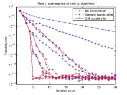
Figure 4.1. This figure shows the results for the experiment described in Subsubsection 4.1.1. We plot $\|A+\hat{I}^{T}\tilde{X}W\|$, the distance of the iterates to $V$, against the number of times we project onto $V$ (4.5) for three different algorithms, namely the method of alternating projections, Algorithm 4.2 (General acceleration) and Algorithm 4.3 (2nd acceleration). For Algorithm 4.2, we test with parameters $q=2,3,4,5,6,7,8$. (Note that $q=1$ corresponds to the alternating projection algorithm). For Algorithm 4.3, we test with parameters $q=1,2,3,4,5$.

4.1.2. Experiment 2

We repeat the experiment in [MDR09] for the case when $M,D,K\in\mathbb{R}^{30\times 30}$ are the matrices

$$M=D=4I_{30\times 30}=\left(\begin{array}[]{cccccc}4&0&0&\cdots&0&0\\ 0&4&0&\cdots&0&0\\ 0&0&4&\cdots&0&0\\ \vdots&\vdots&\vdots&\ddots&\vdots&\vdots\\ 0&0&0&\cdots&4&0\\ 0&0&0&\cdots&0&4\end{array}\right)$$

and $$K=\left(\begin{array}[]{cccccc}1&-1&0&\cdots&0&0\\ -1&2&-1&\cdots&0&0\\ 0&-1&2&\cdots&0&0\\ \vdots&\vdots&\ddots&\ddots&\ddots&\vdots\\ 0&0&\cdots&-1&2&-1\\ 0&0&\cdots&0&-1&1\end{array}\right).$$

The pencil $P(\lambda)=\lambda^{2}M+\lambda D+K$ has 60 eigenvalues, but the eigenvalue that causes the instability is $0$ with eigenvector $\frac{1}{\sqrt{30}}(1,1,\dots,1)^{T}$, and the rest of the spectrum of $P(\lambda)$ is below $-0.0027$. We use $Y_{1}=\frac{1}{\sqrt{30}}(1,1,\dots,1)^{T}$ with targeted eigenvalue $-0.018$.

Our experiments indicate that in one iteration of both Algorithms 4.2 and 4.3, the norm $\|A+\hat{I}^{T}\tilde{X}W\|$ goes down by a factor of $2.4\times 10^{-14}$, essentially reaching convergence within the numerical limits. For the alternating projection algorithm, the decrease is linear, and each iteration reduces the norm $\|A+\hat{I}^{T}\tilde{X}W\|$ by a factor of $0.5$. This experiment once again illustrates the efficiency of the accelerations in Algorithms 4.2 and 4.3.

5. Conclusion

In this paper, we propose acceleration methods for projecting onto the intersection of finitely many affine spaces. This strategy can be applied to general feasibility problems where not only affine spaces are involved, as long as there is more than one affine space.

Acknowledgement.

The author acknowledges very helpful conversations with Lim Chuan Li which led to Propositions 2.3 and 2.4 and Algorithm 2.5. He is grateful to his employer, the National University of Singapore, for his startup grant.

References

- [Agm83] S. Agmon, The relaxation method for linear inequalities, Canad. J. Math. 4 (1983), 479–489.
- [BBL97] H.H. Bauschke, J.M. Borwein, and A.S. Lewis, The method of cyclic projections for closed convex sets in Hilbert space, Recent developments in optimization theory and nonlinear analysis (Jerusalem, 1995), Contemporary Mathematics 204, Amer. Math. Soc., Providence, R.I., 1997, pp. 1–38.
- [BCK06] H.H. Bauschke, P.L. Combettes, and S.G. Kruk, Extrapolation algorithm for affine-convex feasibility problems, Numer. Algorithms 41 (2006), 239–274.
- [BD85] J.P. Boyle and R.L. Dykstra, A method for finding projections onto the intersection of convex sets in Hilbert spaces, Advances in Order Restricted Statistical Inference, Lecture notes in Statistics, Springer, New York, 1985, pp. 28–47.
- [BDHP03] H.H. Bauschke, F. Deutsch, H.S. Hundal, and S.-H. Park, Accelerating the convergence of the method of alternating projections, Trans. Amer. Math. Soc. 355 (2003), no. 9, 3433–3461.
- [DS01] B.N. Datta and D.R. Sarkissian, Theory and computations of some inverse eigenvalue problems for the quadratic pencil, Mathematics, Computer Science, and Engineering I, Contemporary Mathematics Volume 280, Structured Matrices, Amer. Math. Soc., New York, 2001, pp. 221–240.
- [Dyk83] R.L. Dykstra, An algorithm for restricted least-squares regression, J. Amer. Statist. Assoc. 78 (1983), 837–842.
- [ER11] R. Escalante and M. Raydan, Alternating projection methods, SIAM, 2011.
- [GK89] W.B. Gearhart and M. Koshy, Acceleration schemes for the method of alternating projections, J. Comput. Appl. Math. 26 (1989), 235–249.
- [GPR67] L.G. Gubin, B.T. Polyak, and E.V. Raik, The method of projections for finding the common point of convex sets, USSR Comput. Math. Math. Phys. 7 (1967), no. 6, 1–24.
- [Hal62] I. Halperin, The product of projection operators, Acta. Sci. Math. (Szeged) 23 (1962), 96–99.
- [HD97] H.S. Hundal and F. Deutsch, Two generalizations of Dykstra’s cyclic projections algorithm, Math. Programming 77 (1997), 335–355.
- [MDR09] J. Moreno, B.N. Datta, and M. Raydan, A symmetry perserving alternating projection method for matrix model updating, Mech. Syst. Signal Process 23 (2009), 1784–1791.
- [NT14] D. Needell and J. A. Tropp, Paved with good intentions: Analysis of a randomized block Kaczmarz method, Linear Algebra Appl. 441 (2014), 199–221.
- [Pan14a] C.H.J. Pang, Improved analysis of algorithms based on supporting halfspaces and quadratic programming for the convex intersection and feasibility problems, (preprint) (2014).
- [Pan14b] by same author, Set intersection problems: Supporting hyperplanes and quadratic programming, Math. Programming (Online first) (2014).
- [Pie84] G. Pierra, Decomposition through formalization in a product space, Math. Programming 28 (1984), 96–115.
- [vN50] J. von Neumann, Functional operators. II. The geometry of orthogonal spaces., Annals of Mathematics Studies, no. 22., Princeton University Press, Princeton, NJ, 1950, [This is a reprint of mimeograghed lecture notes first distributed in 1933.].
- [XZ02] Jinchao Xu and Ludmil Zikatanov, The method of alternating projections and the method of subspace corrections in Hilbert space, J. Amer. Math. Soc. 15 (2002), no. 3, 573–597.