Deformed one-loop amplitudes in
$\mathcal{N}=4$ super-Yang–Mills theory

1 Introduction and outline

In a series of recent papers, deformations of Yangian invariants in the context of $\mathcal{N}=4$ super-Yang–Mills (sYM) theory have been investigated [1, 2, 3, 4, 5]. As opposed to the undeformed situation, a deformed Yangian invariant allows for nonzero expectation values of the central charge operator for each external leg – which amounts to shifting the helicities of the external particles. Including the hypercharge as well, the underlying symmetry algebra is extended from the Yangian $\mathrm{Y}[\mathfrak{psu}(2,2|4)]$ to $\mathrm{Y}[\mathfrak{u}(2,2|4)]$.

Yangian invariance, however, constrains the allowed deformations by linking the central charges of the external legs to the evaluation parameters of an evaluation representation of the Yangian algebra, thereby encoding a permutation as discussed in refs. [4, 5]. At tree level, the permutation labels a Yangian invariant unambiguously and can be translated into on-shell graphs [6] and $\mathrm{R}$-operators [7].

The relation of deformed Yangian invariants to scattering amplitudes in $\mathcal{N}=4$ sYM theory has been discussed in refs. [3, 4, 5]. All tree-level amplitudes in the maximally-helicity-violating (MHV) sector are represented by a single Yangian invariant, and can thus be deformed. For tree-level amplitudes of higher MHV degree this is not possible any more, as those are composed from several Yangian invariants. The obstruction here is physicality, which demands compatibility between all Yangian invariants contributing to the amplitude: all external legs should have the same data associated to them.

Deformations of the four-point one-loop amplitude have been considered in refs. [1, 2, 3]. In parallel to the tree-level situation, the integrand of the amplitude is a Yangian invariant only for certain deformations. For deformations not leading to a Yangian invariant, one can perform the integration and obtain a result which is reminiscent of the usual expression for the undeformed four-point one-loop amplitude [1, 2]. This fact suggests to use the deformation as a regulator similar to analytic regularization. Keeping Yangian invariance in the integrand, that is, choosing a Yangian-invariant deformation, renders the integration difficult and leads to a vanishing result except for very special deformations [3].

In this note, we investigate how to take deformations to the loop level in a natural way by employing the $\mathrm{R}$-operator formalism described in ref. [7]. We will discuss general features of bubbles in on-shell diagrams in the language of $\mathrm{R}$-operators, which allows to treat the momentum-space properties as well as the Yangian properties simultaneously. From this minimal example, which already exhibits all features of loop amplitudes, we will proceed to deformations of the four-point one-loop integrand of ref. [6] in the language of $\mathrm{R}$-operators.

In particular we compare this deformed amplitude with the four-point one-loop amplitude discussed in refs. [1, 2, 3]. While both integrals lead to the same deformed momentum-space integral, the $\mathrm{R}$-operator language reveals an astonishing fact: they constitute different eigenstates of the monodromy matrix. Thus, either the eigenvalues have to agree, which will be shown to lead to the trivial deformation or the eigenstate has to vanish or diverge. The vanishing result is in agreement with the conclusion drawn in ref. [3].

So the unregulated loop amplitude is a Yangian invariant: it is either zero or infinity. Yangian invariance is only broken by regulating the integral: the infrared divergences arising during the regularization process introduce a scale and thus break conformal invariance.

After the discussion of the four-point one-loop case, we turn our attention to the five-point one-loop amplitude. Based on the Britto–Cachazo–Feng–Witten (BCFW) construction [8, 9] of loop integrands introduced in ref. [10], we consider deformations of the three contributing BCFW-channels in order to arrive at what seems to be a general statement: for loop integrands constructed from several Yangian invariants, there is no consistent deformation if one requires physicality. This argument is analogous to the one used in ref. [5] for tree-level amplitudes in the NMHV sector. For higher-loop amplitudes the situation does not improve.

After a brief review of the necessary techniques for the investigation of deformed scattering amplitudes in sec. 2 we collect previous results on four-point one-loop amplitudes in sec. 3. Section 4 is devoted to the discussion of the integrals occurring in loop constructions on the simple example of a bubble-shaped on-shell graph. In sec. 5 we finally use the $\mathrm{R}$-operator formalism in order to build the four-point one-loop amplitude. We investigate the resulting integral and its branch cut structure in a deformed scenario in order to show that the deformation renders the integral trivial. In sec. 6, we construct the five-point one-loop amplitude following ref. [10] and comment on possible deformations.

2 Amplitudes in $\mathcal{N}=4$ sYM theory, on-shell diagrams and $\mathrm{R}$-operators

In this section we are going to review two descriptions of Yangian invariants relevant in the context of scattering amplitudes in planar $\mathcal{N}=4$ sYM theory: on-shell diagrams and the $\mathrm{R}$-operator formalism. The relations between these two formulations and permutations, which can be used to uniquely label tree-level Yangian invariants, have been thoroughly investigated in refs. [4, 5]. Here we will be rather brief and refer the reader to these references for further details.

Both descriptions of Yangian invariants, $\mathrm{R}$-operators as well as on-shell diagrams, rely on the on-shell superspace [11] with variables $(\lambda^{\alpha},\tilde{\lambda}_{\dot{\alpha}},\tilde{\eta}^{A})$, where Greek and upper case Latin indices label the fundamental representations of $\mathrm{SL}(2)$ and $\mathrm{SU}(4)$ respectively.

Yangian invariants with $n$ external legs are functions defined on the $n$-fold tensor product of on-shell superspace and are annihilated by all generators of the Yangian algebra (see ref. [3] for a short review of Yangian algebras in this context). Extending the algebra $\mathfrak{psu}(2,2|4)$ – which is the algebra underlying planar $\mathcal{N}=4$ sYM theory – with the central charge operator $\mathfrak{C}$ and the hypercharge $\mathfrak{B}$ yields the algebra $\mathfrak{u}(2,2|4)$. Up to reality conditions, the algebra $\mathfrak{u}(2,2|4)$ is equal to $\mathfrak{gl}(4|4)$, which we will be concerned with below. Choosing furthermore an evaluation representation for $\mathrm{Y}[\mathfrak{u}(2,2|4)]$ with evaluation parameters $u_{i}$ leads to a set $(\lambda^{\alpha}_{i},\tilde{\lambda}_{i\dot{\alpha}},\tilde{\eta}^{A}_{i},c_{i},u_{i})$ of external data for each leg, where $c_{i}$ is the eigenvalue of the central charge operator $\mathfrak{C_{i}}$. The total number of $\eta$’s in a $n$-point Yangian invariant determines the variable $k$ labeling the MHV-sector via $k={\textstyle\frac{\#\eta\text{'s}}{4}}$ [11].

On-shell diagrams representing invariants for $\mathrm{Y}[\mathfrak{u}(2,2|4)]$ are composed by gluing two types of deformed three-point vertices [1, 2]

$$\mathcal{A}_{\bullet}=\frac{\delta^{4}(P)\delta^{8}(Q)}{\langle 12\rangle^{1+c_{3}}\langle 23\rangle^{1+c_{1}}\langle 31\rangle^{1+c_{2}}},\qquad\mathcal{A}_{\circ}=\frac{\delta^{4}(P)\delta^{4}(\tilde{Q})}{[12]^{1-c_{3}}[23]^{1-c_{1}}[31]^{1-c_{2}}}\,,$$ (2.1)

where $P:=\sum_{i=1}^{3}\lambda^{\alpha}_{i}\tilde{\lambda}^{\dot{\alpha}}_{i}$ denotes the total four-momentum, whereas $Q:=\sum_{i}\lambda_{i}^{\alpha}\tilde{\eta}_{i}^{A}$ and $\tilde{Q}:=[12]\tilde{\eta}_{3}^{A}+[23]\tilde{\eta}_{1}^{A}+[31]\tilde{\eta}_{2}^{A}$. Each of the building blocks $\mathcal{A}_{\bullet}$ and $\mathcal{A}_{\circ}$ is a Yangian invariant if and only if the following equations are satisfied:

$$\mathcal{A}_{\bullet}: \qquad c_{1}=u_{1}-u_{3},\quad c_{2}=u_{2}-u_{1},\quad c_{3}=u_{3}-u_{2}\,;$$ (2.2)

$$\mathcal{A}_{\circ}: \qquad c_{1}=u_{1}-u_{2},\quad c_{2}=u_{2}-u_{3},\quad c_{3}=u_{3}-u_{1}\,,$$ (2.3)

which implies $\sum_{i}\mathfrak{C}_{i}\mathcal{A}_{\bullet}=\sum_{i}\mathfrak{C}_{i}\mathcal{A}_{\circ}=0$. Combining several of those building blocks in a Yangian-invariant way by gluing leg $V$ to leg $W$ requires (see ref. [3] for a derivation)

$$c_{V}=-c_{W}\quad\text{as well as}\quad u_{V}-{\textstyle\frac{1}{2}}c_{V}=u_{W}-{\textstyle\frac{1}{2}}c_{W}.$$ (2.4)

An on-shell graph represents a Yangian invariant if and only if the system of equations composed from all vertex conditions (cf. eqns. (2.2) and (2.3)) at the vertices as well as the gluing conditions (eqn. (2.4)) for each internal edge is satisfied. This system leads to relations between evaluation parameters and central charges. Generally, solutions to this system of equations are of the form [3, 4, 5]

$$c_{i}=u_{i}-u_{\sigma(i)}$$ (2.5)

where $\sigma(i)$ is the permutation encoded by the on-shell diagram. Instead of solving the linear system, the permutation can also be deduced graphically, by dressing each external leg by two lines: one starting there and the other one ending there. Drawing the lines through the diagram by turning right at each black vertex and left at each white vertex will connect leg $i$ with its image $\sigma(i)$, for example

$$\parbox[c]{104.7915pt}{\leavevmode\hbox{\includegraphics{Fig_5ptperm.mps}}}\qquad\qquad\Bigg{(}\small\begin{matrix}1&2&3&4&5\\ \downarrow&\downarrow&\downarrow&\downarrow&\downarrow\\ 3&4&5&1&2\end{matrix}\Bigg{)}\,.$$ (2.6)

While a unique permutation is associated to each on-shell diagram, there are several different on-shell diagrams encoding the same permutation. Those diagrams are related by square moves and the merger operation depicted in fig. 1. The third operation mentioned in ref. [6], bubble reduction, however, modifies the permutation. The meaning of this operation will become apparent in sec. 4.

$\;\equiv\;$                   $\;\equiv\;$

Figure 1: Square move and merger.

The main players in the $\mathrm{R}$-operator formalism [7] are the Lax operator $\mathrm{L}$ and the $\mathrm{R}$-operator $\mathrm{R}$. While the precise relation between those and Yangian algebras is explained in detail in refs. [4, 5], let us stick with the action of the $\mathrm{R}$-operator on a function defined on several copies of the on-shell superspace, which reads

$$\mathrm{R}_{ab}(u)f(\lambda_{a},\tilde{\lambda}_{a},\tilde{\eta}_{a},\lambda_{b},\tilde{\lambda}_{b},\tilde{\eta}_{b}):=\int_{0}^{\infty}\frac{\mathrm{d}z}{z^{1+u}}f(\lambda_{a}-z\lambda_{b},\tilde{\lambda}_{a},\tilde{\eta}_{a},\lambda_{b},\tilde{\lambda}_{b}+z\tilde{\lambda}_{a},\tilde{\eta}_{b}+z\tilde{\eta}_{a})\ .$$ (2.7)

In terms of these $\mathrm{R}$-operators, an ansatz for a $n$-point tree-level Yangian invariant with MHV-degree $k$ reads

$$\mathcal{Y}=\mathrm{R}_{a_{1}b_{1}}(v_{1})\ldots\mathrm{R}_{a_{2n-4}b_{2n-4}}(v_{2n-4})\Omega\ ,$$ (2.8)

where $\Omega$ is a product of $(n-k)$ $\delta_{a_{i}}$’s and $k$ $\delta_{\text{-}a_{i}}$’s which are defined as

$$\delta_{a}:=\delta^{2}(\lambda_{a}), \delta_{\text{-}a}:=\delta^{2|4}(\tilde{\lambda}_{a}):=\delta^{2}(\tilde{\lambda}_{a})\delta^{4}(\tilde{\eta}_{a})\ .$$ (2.9)

The integrations originating from $2n-4$ $\mathrm{R}$-operators leave four bosonic $\delta$-functions unintegrated, which will combine into momentum conservation $\delta(P)$ later on. As pointed out in sec. 5 below, loop-level amplitudes can be constructed by applying a different number of $\mathrm{R}$-operators to a vacuum state.

The second important object in the $\mathrm{R}$-operator formalism is the Lax operator $\mathrm{L}$. While rigorously defined in ref. [7], here it will be sufficient to note its fundamental relation with $\mathrm{R}$-operators ($u_{ab}=u_{a}-u_{b}$)

$$\mathrm{R}_{21}(u_{12})\mathrm{L}_{1}(u_{1}+{\textstyle\frac{1}{2}}C_{1})\mathrm{L}_{2}(u_{2}+{\textstyle\frac{1}{2}}C_{2}) =\mathrm{L}_{1}(u_{2}+{\textstyle\frac{1}{2}}C_{1})\mathrm{L}_{2}(u_{1}+{\textstyle\frac{1}{2}}C_{2})\mathrm{R}_{21}(u_{12}),$$ (2.10)

$$\mathrm{R}_{12}(u_{12})\mathrm{L}_{1}(u_{1}-{\textstyle\frac{1}{2}}C_{1})\mathrm{L}_{2}(u_{2}-{\textstyle\frac{1}{2}}C_{2}) =\mathrm{L}_{1}(u_{2}-{\textstyle\frac{1}{2}}C_{1})\mathrm{L}_{2}(u_{1}-{\textstyle\frac{1}{2}}C_{2})\mathrm{R}_{12}(u_{12}),$$ (2.11)

which is implied by the Yang–Baxter equation [5]. The equation is to be understood as an operator equation, in which the operators $C_{i}$ measure the central charges on their right-hand side via

$$[C_{a},\mathrm{R}_{ab}(u)]=-u\,\mathrm{R}_{ab}(u), [C_{b},\mathrm{R}_{ab}(u)]=u\,\mathrm{R}_{ab}(u)\quad\text{and}\quad C_{a}\delta_{\pm a}=0\ .$$ (2.12)

The $n$-point monodromy matrix $\mathrm{T}_{n}$ is then defined as a product of Lax-operators

$$\mathrm{T}_{n}:=\mathrm{L}_{1}(u_{1}-{\textstyle\frac{C_{1}}{2}})\ldots\mathrm{L}_{n}(u_{n}-{\textstyle\frac{C_{n}}{2}})\,.$$ (2.13)

Only for certain choices of the parameters $v_{1}\dots v_{2n-4}$ the ansatz eqn. (2.8) will yield a Yangian invariant: the condition analogous to solving the linear system for on-shell graphs is that the ansatz eqn. (2.8) has to be an eigenstate of the monodromy matrix $\mathrm{T}_{n}$ defined in eqn. (2.13) above:

$$\mathrm{T}(\{u_{i}\})\,\mathcal{Y}=\Lambda(\{u_{i}\})\,\mathcal{Y}\ .$$ (2.14)

Commuting the monodromy matrix $\mathrm{T}_{n}$ through the chain of $\mathrm{R}$-operators by means of eqns. (2.10) and (2.11) will fix all parameters $v_{i}$ in the ansatz eqn. (2.8) and furthermore imply eqn. (2.5).

The permutation encoded in a tree-level on-shell graph is the key to expressing a Yangian invariant in the language of $\mathrm{R}$-operators [7, 5]. In order to do so, one has to decompose the permutation into a series of successive swaps and identify the sites to swap with the indices of $\mathrm{R}$-operators $\mathrm{R}_{ab}$. Naturally, there are many different ways of decomposing a permutation into a series of successive swaps. For the tree-level invariants we need to consider series of minimal length. Only after restricting to the shortest possible decompositions one can map a permutation to a class of on-shell diagrams (and thus $\mathrm{R}$-chains) unambiguously. For loop-level invariants, one has to allow for non-minimal decompositions, which obscure the relation between on-shell graphs and permutations.

Finally, let us comment on how to build scattering amplitudes in $\mathcal{N}=4$ sYM theory from Yangian-invariant building blocks. While tree-level amplitudes are sums of Yangian invariants themselves, for loop amplitudes only the integrands exhibit Yangian invariance. As we will see, however, the $\mathrm{R}$-operator formalism provides unregulated, integrated expressions. Since on the one hand those expressions are manifestly Yangian invariant and on the other hand Yangian invariance is broken for loop amplitudes due to infrared divergences, regularization needs to be responsible for breaking Yangian invariance.

As loops will be dealt with in the sections below, let us collect here some facts on tree amplitudes, which have been thoroughly discussed in refs. [1, 2, 3, 4, 5]: in the MHV-sector ($k=2$), any scattering amplitude is directly related to a single Yangian invariant. Imposing the equations ensuring Yangian invariance for this on-shell graphs exactly leads to the relation eqn. (2.5).

For other MHV-sectors ($k>2$), however, there are generically several diagrams contributing to the scattering amplitude. While one can easily determine the permutation associated to each of them, it is unphysical to assign different eigenvalues $c_{i}$ to the same external leg. Imposing equality of all external parameters for all contributing on-shell graphs generically forces all eigenvalues $c_{i}$ to be zero. Thus a deformation is possible only in the MHV sector.

3 Four-point one-loop review

The four-point one-loop MHV gluon amplitude in $\mathcal{N}=4$ sYM theory was first computed in ref. [14] as the low-energy limit of the corresponding string theory result. Later, all one-loop MHV gluon amplitudes have been determined via unitarity in ref. [15]. The result can be expressed as

$$A_{4;2}^{(1)}=\,s\,t\,A_{4;2}^{\mathrm{tree}}I_{4}$$ (3.1)

where $I_{4}$ is the massless box integral

$$I_{4}=\int\frac{\mathrm{d}^{4}q}{q^{2}(q+p_{1})^{2}(q+p_{1}+p_{2})^{2}(q-p_{4})^{2}}\ ,$$ (3.2)

$p_{i},i=1,\dots,4$ are the null external momenta and $s=(p_{1}+p_{2})^{2},\,t=(p_{2}+p_{3})^{2}$ are Mandelstam variables. Using a supersymmetry-preserving regulator such as dimensional reduction, the result is (see ref. [15])

$$A_{4;2}^{(1)}\,=\,-c_{\mathrm{\Gamma}}\,A_{4;2}^{\mathrm{tree}}\biggl{\{}-\frac{2}{\epsilon^{2}}\biggl{[}\biggl{(}\frac{\mu^{2}}{-s}\biggr{)}^{\epsilon}+\biggl{(}\frac{\mu^{2}}{-t}\biggr{)}^{\epsilon}\biggr{]}+\log^{2}\biggl{(}\frac{-s}{-t}\biggr{)}+\pi^{2}\biggr{\}}$$ (3.3)

where

$$c_{\mathrm{\Gamma}}=\frac{(4\pi)^{\epsilon}}{16\pi^{2}}\,\frac{\mathrm{\Gamma}(1+\epsilon)[\mathrm{\Gamma}(1-\epsilon)]^{2}}{\mathrm{\Gamma}(1-2\epsilon)}\ .$$ (3.4)

3.1 On-shell diagrams and all-loop BCFW

In ref. [6], the authors re-derived the four-point one-loop integrand within the on-shell diagram formalism. The amplitude is represented by the highly symmetric diagram in fig. 2, which has been obtained by starting from the forward limit of the six-point NMHV amplitude using the methods of ref. [10] and applying several square moves and mergers afterward. The resulting integrand is expressed as a $\mathrm{dlog}$-form and reads

$$\frac{A_{4;2}^{(1)}}{A_{4;2}^{(\mathrm{tree})}}=\mathrm{dlog}\Bigl{(}\tfrac{\alpha_{1}\langle 31\rangle}{\alpha_{1}\langle 31\rangle+\langle 34\rangle}\Bigr{)}\,\mathrm{dlog}\Bigl{(}\tfrac{\alpha_{2}\langle 13\rangle}{\alpha_{2}\langle 13\rangle+\langle 23\rangle}\Bigr{)}\,\mathrm{dlog}\Bigl{(}\tfrac{\alpha_{3}\langle 13\rangle}{\alpha_{3}\langle 13\rangle+\langle 12\rangle}\Bigr{)}\,\mathrm{dlog}\Bigl{(}\tfrac{\alpha_{4}\langle 31\rangle}{\alpha_{4}\langle 31\rangle+\alpha_{4}\langle 41\rangle}\Bigr{)}\,,$$ (3.5)

where the integration variables $\alpha_{i}$ are BCFW-shifts not fixed by momentum conservation and the on-shell conditions. Alternatively, the above expression can be rewritten in terms of an off-shell integration variable $q$, which denotes the momentum flowing in the loop of the corresponding Feynman diagram. The result reads

$$\frac{A_{4;2}^{(1)}}{A_{4;2}^{(\mathrm{tree})}}=\mathrm{dlog}\biggl{(}\frac{q^{2}}{(q-q^{*})^{2}}\biggr{)}\,\mathrm{dlog}\biggl{(}\frac{(q+p_{1})^{2}}{(q-q^{*})^{2}}\biggr{)}\,\mathrm{dlog}\biggl{(}\frac{(q+p_{1}+p_{2})^{2}}{(q-q^{*})^{2}}\biggr{)}\,\mathrm{dlog}\biggl{(}\frac{(q-p_{4})^{2}}{(q-q^{*})^{2}}\biggr{)}\ ,$$ (3.6)

where $q^{*}=\tfrac{\langle 12\rangle}{\langle 42\rangle}\lambda_{4}\tilde{\lambda}_{1}$ is a solution of the quadruple-cut equation for the box integral [16]. This integrand is equal to

$$\mathrm{d}^{4}q\,\frac{s\,t}{q^{2}\,(q+p_{1})^{2}\,(q+p_{1}+p_{2})^{2}\,(q-p_{4})^{2}}\ ,$$ (3.7)

which is exactly the integrand appearing in eqn. (3.1).

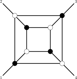
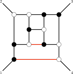
Figure 2: On-shell diagram corresponding to the four-point one-loop amplitude.

3.2 Deformation of the four-point one-loop amplitude

As pointed out in the previous subsection, the four-point one-loop amplitude corresponds to a single on-shell diagram. Therefore it is possible to deform it without taking care for physicality constraints arising from the compatibility of deformations of several Yangian invariants. This was first done in refs. [1, 2]

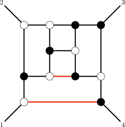
Figure 3: The on-shell diagram corresponding to the deformed one-loop four-point amplitude.

starting from the on-shell graph in fig. 3. The Yangian-invariant deformation of the amplitude reads

$$\mathcal{A}_{4;2}^{(1)}\,=\,s\,t\,A_{4;2}^{\mathrm{tree}}\,\tilde{I}_{4}({a_{i}};s,t)\ ,$$ (3.8)

where $\tilde{I}_{4}({a_{i}};s,t)$ is a box integral with the propagators raised to arbitrary complex powers,

$$\tilde{I}_{4}({a_{i}};s,t)\,=\,\int\mathrm{d}^{4}q\,\frac{1}{[(q)^{2}]^{1+a_{1}}[(q+p_{1})^{2}]^{1+a_{2}}[(q+p_{1}+p_{2})^{2}]^{1+a_{3}}[(q-p_{4})^{2}]^{1+a_{4}}}\ .$$ (3.9)

This form of the integrand is reminiscent of analytic regularization.

Imposing Yangian invariance for the on-shell diagram implies that $\sum_{i}a_{i}=0$ [3]. The explicit computation of this integral (with the Yangian invariance condition enforced) is subtle. If however one does not enforce Yangian invariance, the computation can lead to a finite answer. With a specific choice of external central charges $c_{1}=c_{2}=-c_{3}=-c_{4}=4\epsilon$ (equivalent to choose all $a_{i}=\epsilon$), the explicit computation leads to [1, 2]

$$A_{4;2}^{(1)}\,=\,A_{4;2}^{(\mathrm{tree})}\biggl{(}\frac{[34]}{[12]}\biggr{)}^{4\epsilon}\biggl{[}\frac{1}{\epsilon^{2}}\biggl{(}\frac{s}{t}\biggr{)}^{-2\epsilon}-\frac{1}{2}\biggl{(}\log\frac{s}{t}\biggr{)}^{2}-\frac{7\pi^{2}}{6}+\mathcal{O}(\epsilon)\biggr{]}\,,$$ (3.10)

which bears a striking resemblance with the dimensionally regulated version in eqn. (3.3).

As pointed out before, Yangian invariance for the on-shell diagram is equivalent to demanding $\sum_{i}a_{i}=0$. This condition makes the computation of the integral less straightforward. The result seems to be a distribution with support on the surface $a_{1}-a_{3}=0,\,a_{1}+a_{2}=0$ [3]:

$$A_{4;2}^{(1)} =\,s\,t\,A_{4;2}^{(\mathrm{tree})}\,f(a_{1},a_{2},a_{3})\ ,\quad\text{where}$$ (3.11)

$$f(a_{1},a_{2},a_{3}) =-\delta(a_{1}+a_{2})\delta(a_{2}+a_{3})\frac{1}{s\,t}\biggl{(}\frac{t}{s}\biggr{)}^{a_{1}}\frac{\sin(\pi a_{1})}{a_{1}}\ .$$

That is, for almost all deformations, the integral vanishes.

4 Bubbles

Among the configurations appearing in on-shell diagrams, the bubble takes a special rôle. It reflects the double lines:

$$\parbox[c]{79.497pt}{\leavevmode\hbox{\includegraphics{bubbleperm2.mps}}}\ .$$ (4.1)

In the $\mathrm{R}$-operator language, the above diagram will be produced by the Yangian invariant:

$$\mathrm{R}_{ab}(u_{ab})\mathrm{R}_{ab}(u_{ba})\delta_{a}\delta_{\text{-}b}\,.$$ (4.2)

The very same trivial permutation, however, is represented by $\mathrm{R}_{ba}(u_{ba})\mathrm{R}_{ba}(u_{ab})\delta_{\text{-}a}\delta_{b}$, which corresponds to the following diagram:

$$\parbox[c]{79.497pt}{\leavevmode\hbox{\includegraphics{bubbleperm.mps}}}\,.$$ (4.3)

Employing the definition of the $\mathrm{R}$-operator eqn. (2.7) in the first case eqn. (4.2) leads to

$$\int\frac{\mathrm{d}z_{1}}{z_{1}^{1+u_{ab}}}\int\frac{\mathrm{d}z_{2}}{z_{2}^{1+u_{ba}}}\delta^{2}(\lambda_{a}+(z_{1}+z_{2})\lambda_{b})\delta^{2}(\tilde{\lambda}_{b}-(z_{1}+z_{2})\tilde{\lambda}_{a})\,.$$ (4.4)

Changing variables to $w=z_{1}+z_{2}$ and $z=z_{1}-z_{2}$, performing the integration over $w$ and substituting the remaining variable then leads to

$$\int\frac{\mathrm{d}z}{z^{1+u_{ab}}(D-z)^{1-u_{ab}}}\,\delta(\langle ab\rangle)\delta^{2}(\tilde{\lambda}_{b}-\frac{\lambda^{1}_{a}}{\lambda^{1}_{b}}\tilde{\lambda}_{a})\,,$$ (4.5)

where $D$ is some function of the external kinematics. The above integral exhibits several important features:

• the kinematics is constrained by $\delta(\langle ab\rangle)$. While this renders the kinematics special in the situation of an isolated bubble, it is nothing to worry about, if the bubble is part of a larger on-shell diagram.

• the integration over $z$ means that momentum conservation does not constrain the kinematics completely: the parameter $z$ measures, which part of the momentum flows along the upper and which part along the lower line in the bubble.

• the integration variable $z$ does not appear in the arguments of the $\delta$-function: this allows to consider the integration separately. In fact, this is exactly the situation described by the bubble deletion operation introduced in ref. [6] and mentioned already in sec. 2: one can replace the bubble by a line after factoring out an integration. The link to the integral is provided by the function $D$ of the external kinematics.

  $$\parbox[c]{79.497pt}{\leavevmode\hbox{\includegraphics{bubbledeletion1.mps}}}\quad\rightarrow\quad\parbox[c]{79.497pt}{\leavevmode\hbox{\includegraphics{bubbledeletion2.mps}}}$$ (4.6)

  Note, however, that the operation does not preserve the permutation encoded by the on-shell diagram and thus the Yangian structure, e.g. the flow of the central charges and evaluation parameters is modified by deleting a bubble.

Below we will see that the integral eqn. (4.5) encoded in the bubble is important for investigating deformations of one-loop amplitudes. The close relation of bubbles with loop diagrams becomes apparent in particular by considering the diagram in fig. 4, which is another form of representing the four-point one-loop amplitude. Using the square moves and mergers, it can be transformed

.

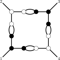
Figure 4: Yet another representation of the four-point one-loop amplitude.

into the diagrams in fig. 2. It is not difficult to see that all these diagrams encode the trivial permutation

$$\Big{(}\begin{smallmatrix}1&2&3&4\\ \downarrow&\downarrow&\downarrow&\downarrow\\ 1&2&3&4\end{smallmatrix}\Big{)}.$$ (4.7)

Contour of integration

Leaving the Grassmann variables aside for a moment, the $\mathrm{R}$-operator as defined in eqn. (2.7) reads

$$R_{ij}(u)\cdot F(\{\lambda,\tilde{\lambda},\tilde{\eta}\}):=\frac{i}{2\sin(\pi u)}\int_{\mathrm{\Gamma}}\frac{\mathrm{d}z}{z^{1+u}}\,F(\lambda_{i}-z\lambda_{j},\tilde{\lambda}_{j}+z\tilde{\lambda}_{i})\ ,$$ (4.8)

Here the contour $\mathrm{\Gamma}$ encircles the branch cut of the integrand (chosen to lie on the positive real axis) going around zero; this open contour is known as the Hankel contour. Already here we encounter a problem, since the Hankel contour does not take into account possible branch cuts from the integrated function $F$ itself. We are going to see below that this is indeed a problem for defining an integration contour for loop amplitudes. However, even for the action of only a single $\mathrm{R}$-operator the situation is not completely clear. One could guess that the Hankel contour is the correct choice in general, since one acts always on single-valued functions; this is however a bit misleading. In order to see this, we study the integral over $z$ in eqn. (4.5). Even though one could argue that this integral represents a degenerate situation (a deformed on-shell diagram with one single bubble), we will see that the same integral appears in the deformed four-point one-loop amplitude below.

The question now is how to choose the integration contour; a naive guess would be simply to generalize the Hankel contour to the closed contour encircling the branch cut, so that the integral picks up the discontinuity of the integrand along the cut. With the change of variables $z=D\zeta$, the integral becomes proportional to (here $\alpha=-u_{ab}$)

$$\oint_{\Gamma}\frac{\mathrm{d}\zeta}{\zeta^{1-\alpha}(1-\zeta)^{1+\alpha}}\ ,$$ (4.9)

where $\Gamma$ is the contour encircling the branch cut between $0$ and $1$. Specifically, $\Gamma=\gamma^{0}_{\epsilon}\cup\gamma_{+}\cup\gamma^{1}_{\epsilon}\cup\gamma_{-}$, where (see fig. 5)

• $\gamma^{0}_{\epsilon},\,\gamma^{1}_{\epsilon}$ are semicircles around the two branch points $0,1$ of radius $\epsilon$;

• $\gamma_{\pm}$ are line segments from $0\pm i\epsilon$ to $1\pm i\epsilon$ (with the correct orientation).

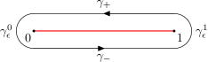
Figure 5: Contour around the branch cut in the $\zeta$ plane

The integrand has no pole at infinity, therefore the evaluation via residue theorem gives zero. Notice, however, that the vanishing of the integral is nontrivial when we consider the single contributions, due to the fact that for $\mathrm{Re}(\alpha)>0$ the integral around $\gamma_{\epsilon}^{1}$ and the contributions from $\gamma_{+}\cup\gamma_{-}$ diverge (and similarly for $\mathrm{Re}(\alpha)<0$ with $\gamma_{\epsilon}^{0}$) . Obviously, even defining the integral purely as the discontinuity around the branch cut (i.e. consider only the contributions along $\gamma_{+}\cup\gamma_{-}$) leads to an ill-defined answer, therefore it seems nontrivial to define an open contour generalizing the Hankel contour.

Notice that the situation considered in the present paragraph is qualitatively different from the one considered in ref. [1, 2]; since in these references the scaling of the deformed integrands depends on the deformation parameters. In our simple case eq. (4.9), the fact that the exponents of the denominator of the integrand sum to zero implies that $z=\infty$ is a regular point and thus the branch-cut can be chosen to lie on the real axis between $0$ and $1$. However, if the exponents sum to a noninteger value, then the integrand would behave as $z^{2-\beta}$ for some $\beta\in\mathbb{C}$ as $|z|\to\infty$. The branch-cut would then lie along $\mathbb{R}\backslash(0,1)$. In that case, the simple integral we consider could be evaluated exactly as a real integral between $0$ and $1$, and would lead to a finite and well-defined answer in a definite region of the space of deformation parameters.

This discussion is done to stress the fact that when considering tree-level amplitudes the contour can be chosen a priori due to the knowledge that all the integrals will be localized on the support of delta functions, but the situation is not as clear when considering integrals beyond tree-level.

As stated at the beginning of this paragraph, we will see that integrals of the form in eqn. (4.9) appear in the computation of the deformed four-point one-loop amplitude. Specifically, eqn. (5.11) from the following section reads

$$\int \frac{\mathrm{d}z_{1}\,\mathrm{d}z_{2}\,\mathrm{d}z_{3}\,\mathrm{d}z_{4}}{z_{1}^{1-u_{14}}\,z_{2}^{1-u_{21}}\,z_{3}^{1-u_{32}}\,z_{4}^{1-u_{43}}}\times$$ (4.10)

$$\quad\times\Bigl{[}\tfrac{\langle 34\rangle}{\langle 34\rangle-z_{1}\langle 31\rangle}\Bigr{]}^{1+u_{14}}\Bigl{[}\tfrac{\langle 23\rangle}{\langle 23\rangle-z_{2}\langle 13\rangle}\Bigr{]}^{1+u_{21}}\Bigl{[}\tfrac{\langle 12\rangle}{\langle 12\rangle-z_{3}\langle 13\rangle}\Bigr{]}^{1+u_{32}}\Bigl{[}\tfrac{\langle 41\rangle}{\langle 41\rangle-z_{4}\langle 31\rangle}\Bigr{]}^{1+u_{43}}$$

The four integrals are completely independent, so we can consider one at a time, for example

$$\int\frac{\mathrm{d}z}{z^{1-a}(\langle 41\rangle-z\langle 31\rangle)^{1+a}}\ ,$$ (4.11)

where the integrand has a single branch cut between $z=0$ and $z=z^{*}:=\frac{\langle 41\rangle}{\langle 31\rangle}$. Each of the integrals in eqn. (4.10) is of the type of eqn. (4.9).

Summing up, it seems then that the deformation leads to well-defined integrands, but the contours of integration are somewhat tricky to define. This fact is immaterial at tree level, since all the integrals are localized on the support of the delta functions. However, at loop level this ambiguity should be resolved in order to attempt to explicitly compute the result.

There are various possible solutions to the contour problem. It is possible to work at the level of the integrand and find a coordinate transformation that leads to a deformed box integral, and then define the usual domain of integration in the loop momentum space, analogous to the computation of refs.[1, 2]; this will be the approach implicitly followed in the following sections. It is also conceivable to define a different contour that crosses the branch cuts of the integrands. The knowledge a priori of the position of the branch cuts of the integrand is then crucial to define such a contour [17].

5 Four-point one-loop calculation

In this section we will discuss the derivation of the deformed one-loop four-point amplitude in the language of $\mathrm{R}$-operators. We will investigate the eigenstates of the monodromy that correspond to fig. 2 and fig. 3 under the dictionary given in [5]. The evaluation of these eigenstates yields integrals which we will map to the deformed box-integral of eqn. (3.9).

Tree level.

Let us start by considering the four-point tree-level amplitude. As shown in [5], the four-point tree-level Yangian invariant can be represented as an eigenfunction of the monodromy matrix of the form

$$\mathcal{A}^{(0)}_{4;2}=\mathrm{R}_{23}(u_{32})\mathrm{R}_{34}(u_{42})\mathrm{R}_{12}(u_{31})\mathrm{R}_{23}(u_{41})\Omega_{++--}.$$ (5.1)

It has eigenvalue $(u_{1}+{\textstyle\frac{1}{2}})(u_{2}+{\textstyle\frac{1}{2}})(u_{3}-{\textstyle\frac{1}{2}})(u_{4}-{\textstyle\frac{1}{2}})$. Its central charges are readily computed to be

$$c_{1}=u_{1}-u_{3}, c_{2}=u_{2}-u_{4}, c_{3}=u_{3}-u_{1}, c_{4}=u_{4}-u_{2},$$ (5.2)

which, using eqn. (2.5), can be directly translated into the permutation that defines this tree-level Yangian invariant. It is simply a shift by two:

$$\Big{(}\begin{smallmatrix}1&2&3&4\\ \downarrow&\downarrow&\downarrow&\downarrow\\ 3&4&1&2\end{smallmatrix}\Big{)}.$$ (5.3)

Employing the definition of the $\mathrm{R}$-operator eqn. (2.7) and the vacuum (2.9) we can evaluate eqn. (5.1) explicitly in terms of spinor-helicity variables

$$\mathcal{A}^{(0)}_{4;2}(\{u_{i}\})=\frac{\delta^{4}(\sum_{i}p_{i})\delta^{8}(\sum_{i}\lambda_{i}\eta_{i})}{\langle 12\rangle^{1+u_{32}}\langle 23\rangle^{1+u_{43}}\langle 34\rangle^{1+u_{14}}\langle 14\rangle^{1+u_{21}}},$$ (5.4)

For $u_{ij}=0$ this expression reduces to the well-known MHV tree-level amplitude for $\mathcal{N}=4$ sYM theory.

One-loop eigenstate.

As discussed in sec. 3, the permutation corresponding to the one-loop diagrams in fig. 2 and fig. 3 is the trivial one. At tree level, the trivial permutation clearly corresponds to the ground state $\Omega$. Nevertheless, we can generate non-trivial Yangian invariants that are associated with these diagrams.

In ref. [5] the explicit map between $\mathrm{R}$-operators and on-shell diagram has been discussed. It is easy to check that the following two states

$$\mathcal{A}_{4;2}^{(1)}=\mathrm{R}_{41}(u_{14})\mathrm{R}_{21}(u_{21})\mathrm{R}_{23}(u_{32})\mathrm{R}_{43}(u_{43})\mathrm{R}_{23}(u_{23})\mathrm{R}_{34}(u_{13})\mathrm{R}_{12}(u_{24})\mathrm{R}_{23}(u_{14})\Omega_{++--},$$ (5.5)

$$\mathcal{B}_{4;2}^{(1)}=\mathrm{R}_{14}(u_{14})\mathrm{R}_{21}(u_{24})\mathrm{R}_{23}(u_{32})\mathrm{R}_{43}(u_{13})\mathrm{R}_{23}(u_{23})\mathrm{R}_{34}(u_{43})\mathrm{R}_{12}(u_{21})\mathrm{R}_{23}(u_{41})\Omega_{++--}$$ (5.6)

exactly give rise to the two on-shell diagrams in fig. 2 and fig. 3 respectively. Notice that the tree-level invariant eqn. (5.1) is represented in the above expressions manifestly by the four rightmost $\mathrm{R}$-operators (up to a redefinition of the spectral parameters).

It can be readily shown that both states are eigenstates of the monodromy matrix with eigenvalues 

$$\mathrm{T}\,\mathcal{A}_{4;2}^{(1)}=(u_{1}+{\textstyle\frac{1}{2}})(u_{2}-{\textstyle\frac{1}{2}})(u_{3}+{\textstyle\frac{1}{2}})(u_{4}-{\textstyle\frac{1}{2}})\mathcal{A}_{4;2}^{(1)},$$ (5.7)

$$\mathrm{T}\,\mathcal{B}_{4;2}^{(1)}=(u_{1}-{\textstyle\frac{1}{2}})(u_{2}-{\textstyle\frac{1}{2}})(u_{3}+{\textstyle\frac{1}{2}})(u_{4}+{\textstyle\frac{1}{2}})\mathcal{B}_{4;2}^{(1)}.$$ (5.8)

The eigenvalues are simply related by interchanging $u_{1}$ and $u_{4}$. Furthermore, it is quickly seen that the central charges vanish

$$c_{i}=0,$$ (5.9)

indicating that eqns. (5.5) and (5.6) indeed correspond to the trivial permutation.

In other words, we have identified Yangian invariants that correspond to the four-point one-loop amplitude. At this point we would like to note that both $\mathcal{A}_{4;2}^{(1)}$ and $\mathcal{B}_{4;2}^{(1)}$ are valid deformations of the one-loop amplitude. If these integrals are well-defined, the fact that they have different eigenvalues implies that they either need to be inequivalent or trivial. Notice furthermore, that apart from applying the parity flip to particles one and four, we could also have applied a flip to any other set of neighboring particles, leading to different deformations. We will come back to this important point at the end of this section.

Integral $\mathcal{A}$.

Having established the relation between the two one-loop eigenstates and their on-shell diagrams, let us evaluate the loop integrals they generate. We will show that both, eqns. (5.5) and (5.6), give rise to the integral eqn. (3.8). We will first treat eqn. (5.5) in great detail and then briefly discuss the derivation of the integral corresponding to eqn. (5.6) afterward.

The Yangian invariant eqn. (5.5) naturally contains eight integrations. The four rightmost $\mathrm{R}$-operators generate the tree-level Yangian invariant and consequently it is convenient to first perform these integrations. This will remove four $\delta$-functions from the vacuum and leaves us with an expression of the form

$$\mathcal{A}_{4;2}^{(1)}=(-1)^{1+u_{41}}\mathcal{A}_{4;2}^{(0)}(\{0\})\,I_{4}(\{u_{i}\}),$$ (5.10)

where the integral $I_{4}(\{u_{i}\})$ is four-dimensional and depends on the integration variables $z_{1},z_{2},z_{3},z_{4}$ from the remaining $\mathrm{R}$-operators. We would like to stress that the factorization in (5.10) can only be done after the application of all R-operators. At the algebraic level, there does not seem to be a way to factor the amplitude into the tree-level amplitude times an integral. Equation (5.10) can be derived straightforwardly by applying eqn. (2.7) to the four-point result eqn. (5.4) . This yields for the integral $I_{4}(\{u_{i}\})$ (cf. [10])

$$\int\frac{\frac{\langle 34\rangle}{\langle 31\rangle}\,\mathrm{d}z_{1}}{z_{1}^{1-u_{14}}\!\left[\!\frac{\langle 34\rangle}{\langle 31\rangle}-z_{1}\right]^{1+u_{14}}}\frac{\frac{\langle 23\rangle}{\langle 13\rangle}\,\mathrm{d}z_{2}}{z_{2}^{1-u_{21}}\!\left[\!\frac{\langle 23\rangle}{\langle 13\rangle}-z_{2}\right]^{1+u_{21}}}\frac{\frac{\langle 12\rangle}{\langle 13\rangle}\,\mathrm{d}z_{3}}{z_{3}^{1-u_{32}}\!\left[\!\frac{\langle 12\rangle}{\langle 13\rangle}-z_{3}\right]^{1+u_{32}}}\frac{\frac{\langle 41\rangle}{\langle 31\rangle}\,\mathrm{d}z_{4}}{z_{4}^{1-u_{43}}\!\left[\!\frac{\langle 41\rangle}{\langle 31\rangle}-z_{4}\right]^{1+u_{43}}}\,.$$ (5.11)

This integral should match the deformed box integral eqn. (3.9). We see that the integrations of the $\mathrm{R}$-operator will play the role of the loop momentum. In order to match this to eqn. (3.9), we have to define what the loop momentum is in our integral. The BCFW recursion relation for loops (or the forward limit) provides a natural candidate: it can be obtained by summing the momenta flowing along the red lines in fig. 2 and fig. 3. The momentum propagating along the various BCFW bridges clearly is a function of the integration parameters $z_{i}$ corresponding to the $\mathrm{R}$-operators that generate the loop integral (the left-most four R-operators). Let us define the shifted momenta [10]

$$\lambda_{\hat{1}}=\lambda_{1}, \tilde{\lambda}_{\hat{1}}=\tilde{\lambda}_{1}+z_{2}\tilde{\lambda}_{2}+z_{1}\tilde{\lambda}_{4},$$

$$\lambda_{\hat{2}}=\lambda_{2}-z_{2}\lambda_{1}-z_{3}\lambda_{3}, \tilde{\lambda}_{\hat{2}}=\tilde{\lambda}_{2},$$

$$\lambda_{\hat{3}}=\lambda_{3}, \tilde{\lambda}_{\hat{3}}=\tilde{\lambda}_{3}+z_{3}\tilde{\lambda}_{2}+z_{4}\tilde{\lambda}_{4},$$

$$\lambda_{\hat{2}}=\lambda_{2}-z_{1}\lambda_{1}-z_{4}\lambda_{3}, \tilde{\lambda}_{\hat{2}}=\tilde{\lambda}_{2}.$$ (5.12)

These expressions can be easily reproduced by acting with the relevant $\mathrm{R}$-operators in eqn. (5.5) on the momentum and removing the measure and integration, i.e. by only considering the shift part from eqn. (2.7). Let us denote such a shift corresponding to the R-operator $\mathrm{R}_{ab}$ by $\mathrm{S}_{ab}(z)$, then

$$\lambda_{\hat{a}}=\mathrm{S}_{41}(z_{1})\mathrm{S}_{21}(z_{2})\mathrm{S}_{23}(z_{3})\mathrm{S}_{43}(z_{4})\lambda_{a}, \tilde{\lambda}_{\hat{a}}=\mathrm{S}_{41}(z_{1})\mathrm{S}_{21}(z_{2})\mathrm{S}_{23}(z_{3})\mathrm{S}_{43}(z_{4})\tilde{\lambda}_{a}.$$ (5.13)

By momentum conservation this results in the following natural expression for the loop momentum

$$q:=\frac{\langle\hat{1}\hat{2}\rangle}{\langle\hat{2}\hat{4}\rangle}\lambda_{\hat{4}}\tilde{\lambda}_{\hat{1}}+z_{1}\lambda_{1}\tilde{\lambda}_{4}.$$ (5.14)

This defines the coordinate transformation between the shift variables $z_{i}$ and the loop momentum. Given this transformation, it is now straightforward to show that

$$I_{4}({a_{i}};s,t)\,=\,\int\mathrm{d}^{4}q\,\frac{s\,t}{[(q)^{2}]^{1+u_{41}}[(q+p_{1})^{2}]^{1+u_{12}}[(q+p_{1}+p_{2})^{2}]^{1+u_{23}}[(q-p_{4})^{2}]^{1+u_{34}}}\ ,$$ (5.15)

which exactly matches eqn. (3.9).

Integral $\mathcal{B}$.

Let us now briefly indicate what happens for the eigenstate eqn. (5.6). The integrand is again of similar type as the integrand of $\mathcal{A}$. Next, we define shifted spinor helicity variables according to the $\mathrm{R}$-operators associated to eqn. (5.6) as

$$\lambda_{\check{a}}=\mathrm{S}_{14}(z_{1})\mathrm{S}_{21}(z_{2})\mathrm{S}_{23}(z_{3})\mathrm{S}_{43}(z_{4})\lambda_{a}, \tilde{\lambda}_{\check{a}}=\mathrm{S}_{14}(z_{1})\mathrm{S}_{21}(z_{2})\mathrm{S}_{23}(z_{3})\mathrm{S}_{43}(z_{4})\tilde{\lambda}_{a},$$ (5.16)

and the corresponding expression for the loop momentum is this time given by

$$q:=\frac{\langle\check{1}\check{2}\rangle}{\langle\check{2}\check{4}\rangle}\lambda_{\check{4}}\tilde{\lambda}_{\check{1}}-z_{1}\lambda_{4}\tilde{\lambda}_{1}.$$ (5.17)

Remarkably, this coordinate transformation maps the integral corresponding to eqn. (5.6) to eqn. (5.15) as well. In other words, eqns. (5.5) and (5.6) correspond to the same function in momentum space but originate from different Yangian invariants.

Summary.

We have shown that both eqns. (5.5) and (5.6) give rise to the same Yangian-deformed box integral. This means that the deformed amplitude is the same for both on-shell diagrams fig. 2 and fig. 3. However, as pointed out in eqn. (5.7), both states have different eigenvalues under the monodromy matrix. This can only happen if either the corresponding states vanish, are ill-defined or if their eigenvalues coincide.

For these two states, the eigenvalues agree exactly when $u_{1}=u_{4}$. However, as was indicated in the beginning of this section, we could have chosen any two adjacent particles and construct the analogue of $\mathcal{B}^{(1)}_{4;2}$. In other words, in order for all these eigenvalues to coincide, we need that $u_{i}=u_{i+1}$. This can only be accomplished when the deformation is trivial, i.e. $u_{ij}=0$, which renders the integral the usual, unregulated box integral.

Indeed in [3] it was shown that the integration of (5.15) on $\mathbb{R}^{4}$ leads to a vanishing result for generic values of the deformation parameters. Furthermore, in [3] the integral seems to have singular support, but we find that even in those particular cases the integral will either vanish or be ill-defined (i.e. divergent). We find that the unregulated integral follows from a manifestly Yangian invariant procedure. However, due to the fact that different Yangian invariants give rise to the same integral, this Yangian invariant seems to be either 0 or divergent.

Finally, as remarked in [5], the eigenvalue of a Yangian invariant corresponds to the hypercharge and its Yangian partners. It is easy to see that the hypercharge of the invariants will start to differ at the second Yangian level only. In turn, this means that our conundrum is closely related to the fact that we extended our algebra not only by the central charge operators $\mathfrak{C}$ but as well by the hypercharge $\mathfrak{B}$.

It is also conceivable that the manipulations of the two expressions in eq. (5.5) and (5.6) are valid at the level of the integral and therefore we should carefully consider the transformation of the contours under the change of variables, as well. However, due to the lack of a precise definition of the contour for the general action of $\mathrm{R}$-operators, we are not able to make any conclusive statement yet.

6 Five-point one-loop amplitude

In this section we discuss the five-point one-loop amplitude. This amplitude is obtained from three on-shell diagrams. We will show that each of these diagrams corresponds to Yangian invariants. However, they have different central charges. It turns out that this implies that they can only be added if the deformation is trivial.

Following the BCFW-recursion relation for loop amplitudes, we find that the diagrams in fig. 6 contribute. The first two diagrams correspond to a forward limit of a seven-point amplitude. The last diagram is an inverse soft limit of the four-point one-loop amplitude discussed in the previous section. The permutations associated to each of the diagrams are

$$\Big{(}\begin{smallmatrix}1&2&3&4&5\\ \downarrow&\downarrow&\downarrow&\downarrow&\downarrow\\ 3&1&2&4&5\end{smallmatrix}\Big{)}\ ,\;\Big{(}\begin{smallmatrix}1&2&3&4&5\\ \downarrow&\downarrow&\downarrow&\downarrow&\downarrow\\ 4&2&1&3&5\end{smallmatrix}\Big{)}\quad\text{and}\quad\Big{(}\begin{smallmatrix}1&2&3&4&5\\ \downarrow&\downarrow&\downarrow&\downarrow&\downarrow\\ 5&2&3&1&4\end{smallmatrix}\Big{)},$$ (6.1)

respectively, which can be quickly derived using the double-line notation introduced in ref. [3].

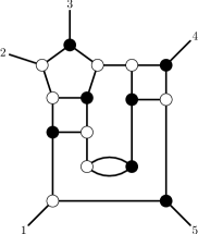
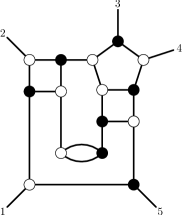
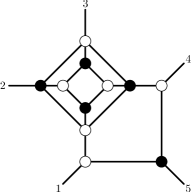
Figure 6: Three channels contributing to the five-point one-loop amplitude.

Let us now spell out the chains of R-operators generating these on-shell diagrams. Define the following three states

$$\mathcal{A}^{(1)}_{5;2}= \mathrm{R}_{51}(u_{15})\mathrm{R}_{45}(u_{41})\mathrm{R}_{54}(u_{54})\mathrm{R}_{12}(u_{52})\mathrm{R}_{51}(u_{24})\mathrm{R}_{34}(u_{13})$$

$$\qquad\mathrm{R}_{15}(u_{34})\mathrm{R}_{45}(u_{23})\mathrm{R}_{42}(u_{52})\mathrm{R}_{32}(u_{21})\Omega_{+-++-}$$ (6.2)

$$\mathcal{B}^{(1)}_{5;2}= \mathrm{R}_{51}(u_{15})\mathrm{R}_{12}(u_{25})\mathrm{R}_{34}(u_{43})\mathrm{R}_{45}(u_{13})\mathrm{R}_{51}(u_{23})\mathrm{R}_{21}(u_{24})$$

$$\qquad\mathrm{R}_{15}(u_{25})\mathrm{R}_{41}(u_{31})\mathrm{R}_{31}(u_{14})\mathrm{R}_{21}(u_{45})\Omega_{-+++-}$$ (6.3)

$$\mathcal{C}^{(1)}_{5;2}= \mathrm{R}_{51}(u_{15})\mathrm{R}_{54}(u_{41})\mathrm{R}_{41}(u_{54})\mathrm{R}_{23}(u_{32})\mathrm{R}_{43}(u_{43})\mathrm{R}_{23}(u_{23})$$

$$\qquad\mathrm{R}_{34}(u_{53})\mathrm{R}_{13}(u_{54})\mathrm{R}_{23}(u_{52})\mathrm{R}_{23}(u_{52})\Omega_{++--+}.$$ (6.4)

It can be shown that they indeed are eigenstates of the monodromy matrix in a way similar to the discussion in Appendix A. Furthermore, it follows directly that these three Yangian invariants generate the on-shell diagrams listed in fig. 6.

In order to study the permutation corresponding to these Yangian invariants, we compute the central charges

$$c_{\mathcal{A}}=\{u_{1}-u_{3},u_{2}-u_{1},u_{3}-u_{2},0,0\},$$

$$c_{\mathcal{B}}=\{u_{1}-u_{4},0,u_{3}-u_{1},u_{4}-u_{3},0\},$$ (6.5)

$$c_{\mathcal{C}}=\{u_{1}-u_{5},0,0,u_{4}-u_{1},u_{5}-u_{4}\}.$$

According to eqn. (2.5) we find that these agree with the permutations listed in eqn. (6.1).

Similar to NMHV amplitudes at tree level, we need to combine several terms to form the full amplitude. Obviously we can only add terms that belong to the same eigenspace, i.e. the central charges must agree. This imposes conditions on the evaluation parameters $u_{i}$ and it is readily checked that implies that $u_{ij}=0$. In other words, there is no deformed five-point one-loop amplitude if one insists on compatibility of the Yangian invariance of the individual terms.

7 Conclusions

In this paper we have constructed and evaluated one-loop diagrams in the language of R-operators. We find that for four points, the same loop integral can be recovered from different on-shell diagrams. However, since formally these two diagrams correspond to different Yangian invariants, it turns out that the integrals either evaluate to zero or diverge.

Except for the four-point one-loop amplitude, there is no consistent deformation for loop amplitudes. The reason is the same, which ruled out the deformed tree amplitudes: if there are several Yangian invariants contributing to a loop-integrand, demanding the same central charges for the external legs of each diagram constrains to the trivial permutation.

Another argument pointing at the subtlety of defining deformed loop amplitudes originates in the complicated branch-cut structure of the integrands. The naive generalization of the Hankel contour leads to ill-defined integrals, as discussed in sec. 4

Without deformation, however, the $\mathrm{R}$-operator formalism leads to exactly the integrands written in ref. [6], which is demonstrated in sec. 5.

Furthermore, we would like to point out that the correspondence between Yangian invariants and permutations will break down at loop level. Indeed, for four points there are only $4!=24$ permutations and clearly at a loop level high enough, this will be smaller than the amount of terms comprising the amplitude.

I’d change to: Finally, we would like to remark that the spectral parameters in the R-operators do not seem to provide a straightforward regularization of loop integrals; not even if we break Yangian invariance only mildly by keeping the arguments of the R-operators general. This is due to the fact that the $\mathrm{R}$-operators have no mass dimension and consequently do not provide an immediate tool to regulate the IR behavior of loop amplitudes. This argument could be circumvented by considering an appropriate contour of integration (as remarked in [17]).

Nevertheless, it would be very useful to further investigate the issue of loop amplitudes in an algebraic language: modifications of the monodromy matrix could still pave the way towards an understanding of the regularization of loop amplitudes.

Acknowledgments.

We would like to thank Niklas Beisert, James Drummond, Jan Plefka, and Cristian Vergu for useful discussions and especially Tomasz Łukowski and Matthias Staudacher for discussions about the contours of integration. The work of MdL and MR is partially supported by grant no. 200021-137616 from the Swiss National Science Foundation.

Appendix A Eigenvalue property

In this section we prove that eqns. (5.5) and (5.6) are eigenstates of the monodromy matrix with eigenvalues given in (5.7). In [7, 5] it was shown that eigenstates of the monodromy matrix respect dihedral symmetry. We will use this and prove that the aforementioned states are eigenstates of $\mathrm{T}$ by showing that they are eigenstates of the shifted monodromy matrix

$$\mathrm{T}_{s}=\mathrm{L}_{2}(u_{2})\mathrm{L}_{3}(u_{3})\mathrm{L}_{4}(u_{4})\mathrm{L}_{1}(u_{1}).$$ (A.1)

We will discuss the procedure for eqn. (5.5) in detail; the computation for eqn. (5.6) is completely analogous. First, we use the rule that two $\mathrm{R}$-operators commute for appropriate indices

$$\mathrm{R}_{ab}(u)\mathrm{R}_{cd}(v)=\mathrm{R}_{cd}(v)\mathrm{R}_{ab}(u), ~{}\mathrm{if}~{}a\neq d~{}\mathrm{and}~{}b\neq c,$$ (A.2)

to rewrite eqn. (5.5) as

$$\mathcal{A}_{4;2}^{(1)}=\mathrm{R}_{41}(u_{14})\mathrm{R}_{23}(u_{32})\mathrm{R}_{43}(u_{43})\mathrm{R}_{23}(u_{23})\mathrm{R}_{34}(u_{24})\mathrm{R}_{21}(u_{21})\mathrm{R}_{12}(u_{24})\mathrm{R}_{23}(u_{14})\Omega_{++--}.$$ (A.3)

It is quickly checked from eqns. (2.10) and (2.11) that $\mathrm{T}_{s}$ can be commuted through the $\mathrm{R}$-operators up to the last three. There we encounter the problem that indices one and two are not adjacent for the shifted monodromy matrix. However, we can use one of the so-called RR$\delta$-rules from [5]

$$\mathrm{R}_{ab}(u)\mathrm{R}_{bc}(v)\delta_{a}\delta_{b}\delta_{\text{-}c}=\mathrm{R}_{bc}(v-u)\mathrm{R}_{ca}(-u)\delta_{\text{-}a}\delta_{b}\delta_{c},$$ (A.4)

together with eqn. (A.2) to find the following way of expressing eqn. (5.5)

$$\mathcal{A}_{4;2}^{(1)}=\mathrm{R}_{41}(u_{14})\mathrm{R}_{23}(u_{32})\mathrm{R}_{43}(u_{43})\mathrm{R}_{23}(u_{23})\mathrm{R}_{34}(u_{24})\mathrm{R}_{13}(u_{14})\mathrm{R}_{23}(u_{12})\mathrm{R}_{23}(u_{21})\Omega_{++--}.$$ (A.5)

Since to the right of $\mathrm{R}_{13}$ there is no $\mathrm{R}$-operator with index four, we find that all operators have neighboring indices and consequently this is an eigenstate of the monodromy matrix. In particular we find

$$\mathrm{T}_{s}\,\mathcal{A}_{4;2}^{(1)}=(u_{1}+{\textstyle\frac{1}{2}})(u_{2}-{\textstyle\frac{1}{2}})(u_{3}+{\textstyle\frac{1}{2}})(u_{4}-{\textstyle\frac{1}{2}})\mathcal{A}_{4;2}^{(1)}.$$ (A.6)

The exact same considerations work for eqn. (5.6) as well since they only differ by a parity-flip of the first $\mathrm{R}$-operator, which does not spoil the property that it is an eigenstate of shifted monodromy matrix. This results in

$$\mathrm{T}_{s}\,\mathcal{B}_{4;2}^{(1)}=(u_{1}-{\textstyle\frac{1}{2}})(u_{2}-{\textstyle\frac{1}{2}})(u_{3}+{\textstyle\frac{1}{2}})(u_{4}+{\textstyle\frac{1}{2}})\mathcal{B}_{4;2}^{(1)}.$$ (A.7)

We see that the eigenvalues are simply related by interchanging $u_{1}\leftrightarrow u_{4}$. Because the central charges are vanishing for both states, we find that the eigenvalues of $\mathrm{T}_{s}$ and the normal monodromy matrix $\mathrm{T}$ coincide. This proves eqn. (5.7).

References

- [1] L. Ferro, T. Lukowski, C. Meneghelli, J. Plefka and M. Staudacher, “Harmonic R-matrices for scattering amplitudes and spectral regularization”, Phys.Rev.Lett. 110, 121602 (2013), arxiv:1212.0850.
- [2] L. Ferro, T. Lukowski, C. Meneghelli, J. Plefka and M. Staudacher, “Spectral parameters for scattering amplitudes in N=4 super Yang–Mills theory”, arxiv:1308.3494.
- [3] N. Beisert, J. Broedel and M. Rosso, “On Yangian-invariant regularisation of deformed on-shell diagrams in N=4 super-Yang–Mills theory”, arxiv:1401.7274.
- [4] N. Kanning, T. Lukowski and M. Staudacher, “A shortcut to general tree-level scattering amplitudes in N=4 SYM via integrability”, arxiv:1403.3382.
- [5] J. Broedel, M. de Leeuw and M. Rosso, “A dictionary between R-operators, on-shell graphs and Yangian algebras”, arxiv:1403.3670.
- [6] N. Arkani-Hamed, J. L. Bourjaily, F. Cachazo, A. B. Goncharov, A. Postnikov et al., “Scattering amplitudes and the positive Grassmannian”, arxiv:1212.5605.
- [7] D. Chicherin, S. Derkachov and R. Kirschner, “Yang–Baxter operators and scattering amplitudes in N=4 super-Yang–Mills theory”, arxiv:1309.5748.
- [8] R. Britto, F. Cachazo and B. Feng, “New recursion relations for tree amplitudes of gluons”, Nucl.Phys. B715, 499 (2005), hep-th/0412308.
- [9] R. Britto, F. Cachazo, B. Feng and E. Witten, “Direct proof of tree-level recursion relation in Yang–Mills theory”, Phys.Rev.Lett. 94, 181602 (2005), hep-th/0501052.
- [10] N. Arkani-Hamed, J. L. Bourjaily, F. Cachazo, S. Caron-Huot and J. Trnka, “The all-loop integrand for scattering amplitudes in planar N=4 SYM”, JHEP 1101, 041 (2011), arxiv:1008.2958.
- [11] V. Nair, “A current algebra for some gauge theory amplitudes”, Phys.Lett. B214, 215 (1988).
- [12] N. Beisert and B. U. Schwab, “Bonus Yangian symmetry for the planar S-Matrix of N=4 super Yang–Mills”, Phys.Rev.Lett. 106, 231602 (2011), arxiv:1103.0646.
- [13] D. Kosower, R. Roiban and C. Vergu, “The six-Point NMHV amplitude in maximally supersymmetric Yang–Mills Theory”, Phys.Rev. D83, 065018 (2011), arxiv:1009.1376.
- [14] M. B. Green, J. H. Schwarz and L. Brink, “N=4 Yang–Mills and N=8 supergravity as limits of string theories”, Nucl.Phys. B198, 474 (1982).
- [15] Z. Bern, L. J. Dixon, D. C. Dunbar and D. A. Kosower, “One loop -point gauge theory amplitudes, unitarity and collinear limits”, Nucl.Phys. B425, 217 (1994), hep-ph/9403226.
- [16] Z. Bern, V. Del Duca, L. J. Dixon and D. A. Kosower, “All non-maximally-helicity-violating one-loop seven-gluon amplitudes in N=4 super-Yang–Mills theory”, Phys.Rev. D71, 045006 (2005), hep-th/0410224.
- [17] Staudacher, M., talk given at the XIX Itzykson Conference, Amplitudes 2014, a Claude Itzykson memorial conference, June 10 - 13, 2014, CEA Saclay, http://ipht.cea.fr/en/Meetings/Itzykson2014/talks/Staudacher-Itzykson19.pdf.