Study of Inflationary Generalized Cosmic Chaplygin Gas for Standard and Tachyon Scalar Fields

Abstract

We consider an inflationary universe model in the context of generalized cosmic Chaplygin gas by taking matter field as standard and tachyon scalar fields. We evaluate the corresponding scalar fields and scalar potentials during intermediate and logamediate inflationary regimes by modifying the first Friedmann equation. In each case, we evaluate the number of e-folds, scalar as well as tensor power spectra, scalar spectral index and important observational parameter, i.e., tensor-scalar ratio in terms of inflatons. The graphical behavior of this parameter shows that the model remains incompatible with WMAP7 and Planck observational data in each case.

Keywords: Inflation; Slow-roll approximation.
PACS: 05.40.+j; 98.80.Cq.

1 Introduction

A combination of different cosmic probes like type Ia supernova, the large scale structure (LSS), cosmic microwave background (CMB) and WMAP confirmed that our universe is experiencing accelerating expansion [1]. Little is known about the origin of this cosmic stage which may be due to dark energy (DE) (with large negative pressure). It fills two-third of the whole cosmic energy and remaining portion is almost occupied by the dark matter (DM). A tiny constant $\Lambda$ is the simplest identification of DE which suffers with fine-tuning and cosmic coincidence issues. The dynamical nature of DE is divided into scalar field models (quintessence, phantom, k-essence etc.) [2] and interacting DE models (Chaplygin gas (CG), holographic DE, Ricci DE etc.) [3].

Chaplygin gas (a unification of DE and DM) is considered to be an interesting alternative description of accelerating expansion. It has negative pressure obeying equation of state (EoS) $P=-\frac{A}{\rho},~{}A>0$ and positive speed of sound which is a powerful tool to discriminate between various DE models. The velocity of sound approaches to the velocity of light for late time while negligibly small for early times. The energy density of CG smoothly varies from matter dominated era to a constant point, i.e., $\Lambda$ cold DM ($\Lambda$CDM) in the future universe [4]. Many people carried out cosmology of different models of CG like generalized CG (GCG) [5], modified CG (MCG) [6] and generalized cosmic CG (GCCG) [7] etc. Kamenshchik et al. [8] considered FRW universe composed of CG and showed that resulting evolution of the universe is in agreement with the current observation of cosmic acceleration.

Recently, a great amount of work has been done in investigating the inflationary universe model with a tachyon field. This field might be responsible for cosmological inflation in the early evolution of the universe due to tachyon condensation near the top of the effective scalar potential [9], which could also add some new form of cosmological DM at late times [10]. Gibbons [11] was the first who studied cosmological implications of this rolling tachyon. It is quite natural to consider some scenarios in which inflation is driven by the rolling tachyon. The CG emerges as an effective fluid of generalized d-brane in a (d+1, 1) spacetime, where the action can be written as a generalized Born-Infeld action [12]. These models (CG and tachyon) have extensively been studied in the literature [13]. In Chaplygin inspired inflationary universe model, the standard inflaton field usually drives inflation where the energy density can be extrapolated for obtaining a successful inflation period [14]. Del Campo and Herrera [15] studied warm-Chaplygin and tachyon-Chaplygin inflationary universe model. Monerat et al. [16] explored dynamics of the early universe and initial conditions for an inflationary model with radiation and CG.

The standard cosmology explains observations of CMB radiations in an elegant way but early phase of the universe is still facing some long-standing issues like horizon problem, flatness, numerical density of monopoles and the origin of fluctuations [17]. The inflationary models present better description of the early universe which also provide the most compelling solution of these problems. Inflation can provide an elegant mechanism to explain causal interpretation of the origin of the observed anisotropy of CMB and inhomogeneity for structure formation. Scalar field models composed of kinetic and potential terms coupled to gravity produce dynamical framework and act as a source for inflation. These models have ability to interpret the distribution of LSS and observed anisotropy of CMB radiations comprehensively in inflationary era [18].

Inflationary era is divided into slow-roll and reheating epochs. During slow-roll approximation, the universe inflates as the interactions between inflatons and other fields become negligibly small and potential energy dominates the kinetic energy. After this period, the universe enters into last stage of inflation, i.e., reheating era in which kinetic and potential energies are comparable. Here the inflaton starts to oscillate around the minimum of its potential while losing its energy to massless particles. Inflationary model is usually discussed in intermediate and logamediate scenarios.

During intermediate era, the universe expands at the rate slower than the standard de Sitter inflation while faster than power-law inflation [19]. Setare and Kamali [20] have discussed warm vector inflation in this scenario for FRW model and proved that the results are compatible with WMAP7 data [21]. The same authors [22] also dealt with warm inflation using gauge fields in intermediate as well as logamediate scenarios. In a recent paper [23], we have studied warm vector inflation in locally rotationally symmetric Bianchi type I universe model and verified its compatibility with WMAP7 data.

The study of inflationary epoch with intermediate and logamediate scale factors lead to over-lasting forms of the potential which agree with tachyon potential properties. Moreover, the study of warm inflation as a mechanism gives an end for standard and tachyon inflation. This motivated us to consider inflationary model with these two potentials. Recently, Herrera et al. [24] studied intermediate GCG inflationary universe model with standard as well as tachyon scalar fields and checked its compatibility with WMAP7 data. Since GCCG is less constrained as compared to MCG and GCG and is capable of adapting itself to any domain of cosmology depending upon the choice of parameters. Thus it has more universal character and the big-rip singularity can easily be avoided in this model. These generalizations of CG can lead to significant changes in the early universe. It would be interesting to check the behavior of inflationary universe with GCCG using standard and tachyon scalar fields during intermediate as well as logamediate epochs. This work can recover all the previous existing models of CG.

The paper is arranged in the following format. In the next section, we modify the first Friedmann equation and find solutions of standard and tachyon scalar fields as well as their corresponding potentials. We also provide the slow-roll parameters, number of e-folds, scalar and tensor power spectra, scalar spectral index and tensor-scalar ratio. In section 3, we develop our model in intermediate and logamediate inflation with both types of scalar fields. We conclude our discussion in the last section.

2 Inflation with Standard and Tachyon Scalar Fields

In this section, we modify the first Friedmann equation in the context of GCCG inflationary universe model. We choose standard and tachyon scalar fields as matter content of this universe and calculate both scalar fields and their corresponding potentials. We also formulate some important perturbed parameters.

González-Diaz [7] introduced GCCG model in such a way that the resulting models can be made stable and physical even when the vacuum fluid satisfies the phantom energy condition. It has the following exotic EoS

$$P=-\rho^{-\alpha}\left[C+(\rho^{1+\alpha}-C)^{-\omega}\right],$$ (1)

where $C=\frac{A}{1+\omega}-1,~{}A$ is either positive or negative constant, $\alpha$ is any positive constant and $-l<\omega<0$, $l>1$. This EoS reduces to GCG model as $\omega\rightarrow 0$. The corresponding energy density is obtained by integrating the energy conservation equation of the GCCG as follows

$$\rho=\left[C+\left(1+\frac{B}{a^{3(1+\alpha)(1+\omega)}}\right)^{\frac{1}{1+\omega}}\right]^{\frac{1}{1+\alpha}},$$ (2)

with scale factor $a$ and $B$ is the integration constant. The gravity dynamics during inflation leads to modify the first Friedmann equation as [12]

$$H^{2}=\frac{\kappa}{3(1+\omega)}\left[C+\rho^{(1+\alpha)(1+\omega)}_{\phi}\right]^{\frac{1}{1+\alpha}},$$ (3)

where $\kappa=\frac{8\pi}{m^{2}_{p}},~{}m_{p}$ is the reduced Planck mass and $\rho_{\phi}$ is the energy density of the scalar field. This modification is dubbed as Chaplygin inspired inflation.

We take two types of scalar fields for $\rho_{\phi}$, i.e., standard and tachyon scalar fields. The energy conservation of a scalar field is

$$\dot{\rho}_{\phi}+3H(\rho_{\phi}+P_{\phi})=0,$$ (4)

where the associated standard energy density and pressure are given as

$$\rho_{\phi}=\frac{\dot{\phi}^{2}}{2}+V(\phi),\quad P_{\phi}=\frac{\dot{\phi}^{2}}{2}-V(\phi).$$

Using $\rho_{\phi}$ and $P_{\phi}$, the above equation is equivalent to the equation of motion of the standard scalar field as follows

$$\ddot{\phi}+3H\dot{\phi}+V^{\prime}(\phi)=0,$$ (5)

where $\prime$ denotes derivative with respect to $\phi$. Equations (3) and (4) yield

$$\dot{\phi}^{2}=-\left(\frac{2\dot{H}}{\kappa}\right)\left(\frac{3H^{2}}{\kappa}\right)^{\alpha}\left(\frac{3H^{2}}{\kappa}\right)^{(1+\alpha)\psi}\left[1-\frac{A}{(1+\omega)}\left(\frac{\kappa}{3H^{2}}\right)^{1+\alpha}\right]^{\psi},$$ (6)

where $\psi=\left[\frac{1}{(1+\alpha)(1+\omega)}-1\right]$. The scalar potential is obtained by substituting $\rho_{\phi}$ from (3) and $\dot{\phi}^{2}$ from (6) in the formula for energy density of standard scalar field as follows

$$V(t) = (1+\omega)\left[\left(\frac{3H^{2}}{\kappa}\right)^{1+\alpha}-\frac{A}{(1+\omega)}\right]^{\psi+1}+\left[\frac{\dot{H}}{\kappa}\left(\frac{3H^{2}}{\kappa}\right)^{\alpha+(1+\alpha)\psi}\right.$$ (7)

$$\times \left.\left[1-\frac{A}{(1+\omega)}\left(\frac{\kappa}{3H^{2}}\right)^{1+\alpha}\right]^{\psi}\right].$$

The above two solutions reduce to typical standard inflation for $\alpha,~{}A,~{}\omega\rightarrow 0$, pure CG model for $\alpha,~{}\omega\rightarrow 0$ and GCG model for $\omega\rightarrow 0$ [25].

The energy density and pressure of tachyon field are

$$\rho_{\phi}=\frac{V(\phi)}{\sqrt{1-{\dot{\phi}}^{2}}},\quad P_{\phi}=V(\phi)\sqrt{1-{\dot{\phi}}^{2}}.$$ (8)

Using Eq.(4), we obtain the corresponding equation of motion

$$\frac{\ddot{\phi}}{1-\dot{\phi}^{2}}+3H\dot{\phi}+\frac{V^{\prime}(\phi)}{V(\phi)}=0.$$ (9)

Equations (3) and (9) provide the time derivative of tachyon field as follows

$$\dot{\phi}^{2}=-\left(\frac{2\dot{H}}{\kappa}\right)\left(\frac{3H^{2}}{\kappa}\right)^{\alpha}\frac{1}{(1+\omega)}\left[\left(\frac{3H^{2}}{\kappa}\right)^{1+\alpha}-\frac{A}{1+\omega}\right]^{-1}.$$ (10)

Using above equation with (3) in $\rho_{\phi}$ given in (8), we have tachyon potential

$$V(t) = (1+\omega)^{\frac{1}{2}}\sqrt{1+\frac{2\dot{H}}{\kappa}\left(\frac{3H^{2}}{\kappa}\right)^{\alpha}\frac{1}{(1+\omega)}\left[\left(\frac{3H^{2}}{\kappa}\right)^{1+\alpha}-\frac{A}{1+\omega}\right]^{-1}}$$ (11)

$$\times \left[\left(\frac{3H^{2}}{\kappa}\right)^{1+\alpha}-\frac{A}{(1+\omega)}\right]^{\psi+1}.$$

The dimensionless slow-roll parameters $\epsilon,\eta$ and number of e-folds are defined as

$$\epsilon=-\frac{\dot{H}}{H^{2}},\quad\eta=-\frac{\ddot{H}}{H\dot{H}},\quad N=A\int^{t_{2}}_{t_{1}}Hdt;\quad A>0,$$ (12)

where $t_{1}$ and $t_{2}$ being the starting and ending cosmic time of inflationary era.

Now we define scalar and tensor power spectra for GCCG inflationary model with standard and tachyon scalar fields. The power spectrum as a function of wave number $(k)$ is the basic tool to quantify fluctuation’s variance produced by inflatons. In order to calculate scalar perturbation, a gauge invariant quantity, $\zeta=H+\frac{\delta\rho}{\dot{\rho}}$, is introduced [26]. This quantity almost remains constant on super-horizon scales but reduces to curvature perturbation on a slice of uniform density. This fundamental characteristic is a consequence of stress-energy conservation and independent of gravitational dynamics which keeps it unchanged in Chaplygin inflationary model [27]. Thus the power spectrum corresponds to curvature spectrum and can be written as $\mathcal{P_{R}}=\langle\zeta^{2}\rangle$ [24]. Since the curvature perturbations act as comoving curvature perturbation on the slices of uniform density, so for spatially flat gauge fields, we have [28]

$$\mathcal{P_{R}}\simeq H^{2}\frac{(\delta\phi)^{2}}{(\dot{\phi})^{2}};\quad|\delta\phi|=\frac{H}{2\pi}\quad\Rightarrow\quad\mathcal{P_{R}}\simeq\frac{H^{4}}{4\pi^{2}\dot{\phi}^{2}}.$$ (13)

The scalar power spectrum for tachyon field using slow-roll approximation $((\dot{\phi})^{2}<<V(\phi))$ has the form [29]

$$\mathcal{P_{R}}\simeq\left(\frac{H^{2}}{2\pi\dot{\phi}}\right)^{2}\frac{1}{Z_{s}};\quad Z_{s}=V(1-(\dot{\phi})^{2})^{-\frac{3}{2}}\approx V(\phi).$$ (14)

The tensor perturbation generating gravitational waves and scalar spectral index, $n_{s}$ are defined as

$$\mathcal{P}_{g}=8\kappa\left(\frac{H}{2\pi}\right)^{2},\quad n_{s}-1=-\frac{d\ln\mathcal{P_{R}}(k)}{d\ln k}.$$ (15)

The tensor-scalar ratio (an observational quantity) for both standard and tachyon scalar fields, respectively, is

$$r=\frac{\mathcal{P}_{g}}{\mathcal{P_{R}}}=8\kappa\left(\frac{\dot{\phi}}{H}\right)^{2},\quad r=8\kappa\left(\frac{\dot{\phi}}{H}\right)^{2}V.$$ (16)

According to the observations of WMAP+BAO (baryon acoustic oscillations)+SN, the scalar spectral index and perturbed scalar power spectrum are constrained to $0.96\leq n_{s}\leq 1.002$ (95% C.L.) and $\mathcal{P_{R}}(k_{0}=0.002Mpc^{-1})=(2.445\pm 0.096)\times 10^{-9}$, respectively [18] while tensor power spectrum cannot be constrained directly. In this context, physical acceptable range of tensor-scalar ratio is determined, i.e., $r<0.36$ (95% C.L.) which represents the expanding universe.

3 Intermediate and Logamediate Inflation

Here, GCCG inflationary universe model is developed in intermediate and logamediate eras using standard and tachyon scalar fields. We reconstruct solutions of both fields, their potentials and perturbed parameters (found in the above section) during these two scenarios.

3.1 Standard Scalar Field

First, we take standard scalar field as matter content of the inflationary universe and discuss in intermediate as well as logamediate scenarios.

3.1.1 Intermediate Inflation

This era is motivated by string/M theory and is one of the exact solutions of the inflationary cosmology. The 4-dimensional Gauss Bonnet interaction with dynamical dilatonic scalar coupling leads to an intermediate form of the scale factor [30]

$$a(t)=a_{0}\exp(At^{f}),\quad A>0,~{}0<f<1,$$ (17)

where $a_{0}$ is the value of scale factor at $t=0$. Using Eq.(17) in (6), we obtain the following solution of standard scalar field $\phi$

$$\phi(t)-\phi_{0}=\frac{2\left(\frac{2}{\kappa}(Af)(1-f)\left(\frac{3(Af)^{2}}{\kappa}\right)^{\alpha+(1+\alpha)\psi}\right)^{\frac{1}{2}}}{f+2(f-1)\left[\alpha+(1+\alpha)\psi\right]}t^{\frac{f+2(f-1)\left[\alpha+(1+\alpha)\psi\right]}{2}},$$ (18)

where $\phi_{0}$ is an integration constant at $t=0$. Without loss of generality, we can take $\phi_{0}=0$ to express time in terms of scalar field as

$$t=\left[\frac{\phi\left[f+2(f-1)\left[\alpha+(1+\alpha)\psi\right]\right]}{2\left(\frac{2}{\kappa}(Af)(1-f)\left(\frac{3(Af)^{2}}{\kappa}\right)^{\alpha+(1+\alpha)\psi}\right)^{\frac{1}{2}}}\right]^{\frac{2}{f+2(f-1)\left[\alpha+(1+\alpha)\psi\right]}}.$$ (19)

Using Eq.(17), standard scalar potential (7) is as follows

$$V(\phi) = (1+\omega)\left[\left[\frac{\phi\left[f+2(f-1)\left[\alpha+(1+\alpha)\psi\right]\right]}{2\left(\frac{2}{\kappa}(Af)(1-f)\left(\frac{3(Af)^{2}}{\kappa}\right)^{\alpha+(1+\alpha)\psi}\right)^{\frac{1}{2}}}\right]^{\frac{4(f-1)(1+\alpha)}{f+2(f-1)\left[\alpha+(1+\alpha)\psi\right]}}\right.$$ (20)

$$\times \left(\frac{3(Af)^{2}}{\kappa}\right)^{1+\alpha}-\left.\frac{A}{1+\omega}\right]^{\psi+1}.$$

The slow-roll parameters and number of e-folds are found through Eq.(12) using Eq.(19). Another scalar field $\phi_{1}$ is produced at the beginning of inflation epoch, where $\epsilon=1$. The standard scalar power spectrum during intermediate era can be calculated by inserting Eq.(6) in (13) and then using Eq.(19), it follows that

$$\mathcal{P_{R}} = \frac{(Af)^{3}}{(1-f)}\left(\frac{\kappa}{8\pi^{2}}\right)\mu^{\frac{3f-2}{f}}\left[\mu^{\frac{2(f-1)}{f}}\left(\frac{3}{\kappa}\right)(Af)^{2}\right]^{-\alpha-(1+\alpha)\psi}\left[1-\frac{A}{1+\omega}\right.$$ (21)

$$\times \left.\mu^{\frac{2(1-f)(1+\alpha)}{f}}\left(\frac{\kappa}{3(Af)^{2}}\right)^{1+\alpha}\right]^{-\psi},$$

where $\mu=\frac{1+f(N-1)}{Af}$. Equations (15) provides $P_{g}$ and $n_{s}$ as a function of $N$, respectively

$$n_{s}-1 = \frac{2-3f}{Af}\mu^{-1}+2\left[-\alpha-(1+\alpha)\psi\right]\left(\frac{f-1}{f}\right)\mu^{\frac{(1-f)}{f}}$$ (22)

$$- \psi\left[1-\frac{A}{1+\omega}\left(\frac{\kappa}{3(Af)^{2}}\right)^{1+\alpha}\mu^{\frac{2(1-f)(1+\alpha)}{f}-1}\right]\left[\frac{2(f-1)(1+\alpha)}{f(1+\omega)}\right.$$

$$\times \left.\left(\frac{\kappa}{3(Af)^{2}}\right)^{1+\alpha}\mu^{\frac{2(1-f)(1+\alpha)}{f}-1}\right],\quad P_{g}=\left(\frac{2\kappa}{\pi^{2}}\right)(Af)^{2}\mu^{\frac{2(f-1)}{f}}.$$

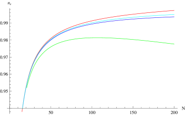
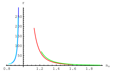
Figure 1: (left) $n_{s}$ versus $N$, (right) tensor-scalar ratio versus $n_{s}$ for $A=8.225\times 10^{2},~{}\alpha=0.775,~{}\omega=-0.8,~{}g=\frac{1}{2},~{}k=1$ (red); $A=2.635\times 10^{2},~{}\alpha=0.81,~{}\omega=-1.5$ (green); $A=8.407\times 10^{2},~{}\alpha=0.85,~{}\omega=-1.7$ (blue) and $A=8.407\times 10^{2},~{}\alpha=0,~{}\omega=0$ (zinc) in intermediate scenario.

Using Eqs.(21) and (22), the tensor-scalar ratio has the form

$$r(N) = 16\left(\frac{1-f}{Af}\right)\mu^{-1}\left[\left(\frac{3}{\kappa}\right)(Af)^{2}\mu^{\frac{2(f-1)}{f}}\right]^{\alpha+(1+\alpha)\psi}\left[1-\frac{A}{1+\omega}\right.$$

$$\times \left.\left(\frac{\kappa}{3(Af)^{2}}\right)^{1+\alpha}\mu^{\frac{2(1-f)(1+\alpha)}{f}}\right]^{\psi}.$$

The left panel of Figure 1 shows an increasing behavior of $n_{s}$ with respect to $N$. The observed value of $n_{s}=0.96$ corresponds to $N\approx 20$ for all values of parameters which indicates physical compatibility of these model parameters with WMAP7 data. The right graph of Figure 1 shows that red and green $r-n_{s}$ trajectories are decreasing while other two are increasing. We see that none of the case is compatible with WMAP7 data as the observed value $0.96\leq n_{s}\leq 1$ does not lie in the region $r\leq 0.36$ during intermediate scenario.

3.1.2 Logamediate Inflation

Logamediate inflationary era is motivated by imposing weak general conditions on the indefinite expanding cosmological models. It has been proved that the power spectrum is either red or blue tilted for this type of inflation. The scale factor satisfies [31]

$$a(t)=a_{0}\exp[A(\ln t)^{\lambda}],\quad\lambda>1.$$ (23)

For $\lambda=1$, it is converted to power-law inflation. During logamediate inflation, Eq.(6) has the following solution

$$\phi(t)-\phi(t_{0}) = -\Xi(t)\left[\left(\frac{2}{\kappa}\right)\left(\frac{3}{\kappa}\right)^{\alpha+(1+\alpha)\psi}(A\lambda)^{1+2(\alpha+(1+\alpha)\psi)}\right]^{\frac{1}{2}}$$ (24)

$$\times \left[\frac{A}{1+\omega}\left(\frac{\kappa}{3}\right)^{1+\alpha}(A\lambda)^{-2(1+\alpha)}\right]^{\frac{\psi}{2}},$$

where $\Xi(t)=\gamma[\frac{\lambda+2\alpha(\lambda-1)}{2},\alpha\ln t]$ ($\gamma$ is incomplete gamma function). From the above equation, $t$ is calculated in terms of $\phi$ as

$$t = \Xi^{-1}\left[-\phi\left[\left(\frac{2}{\kappa}\right)\left(\frac{3}{\kappa}\right)^{\alpha+(1+\alpha)\psi}(A\lambda)^{1+2(\alpha+(1+\alpha)\psi)}\right]^{-\frac{1}{2}}\right.$$ (25)

$$\times \left.\left[\frac{A}{1+\omega}\left(\frac{\kappa}{3}\right)^{1+\alpha}(A\lambda)^{-2(1+\alpha)}\right]^{-\frac{\psi}{2}}\right].$$

The corresponding Hubble parameter, standard scalar potential, slow-roll as well as number of e-folds can be calculated as in the intermediate case.

The scalar and tensor perturbed parameters in terms of $N$ can be written as

$$\mathcal{P_{R}} = \left(\frac{\kappa}{8\pi^{2}}\right)\left(\frac{\kappa}{3}\right)^{\alpha+(1+\alpha)\psi}\frac{(A\lambda)^{3-2(\alpha+(1+\alpha)\psi)}}{(1-\lambda)}\varepsilon^{\frac{3\lambda-2(\lambda-1)(\alpha+(1+\alpha)\psi)-2}{\lambda}}$$

$$\times \exp\left[\left(\frac{2(\alpha+(1+\alpha)\psi)-1}{\lambda}\right)\varepsilon\right]\left[1-\frac{A}{1+\omega}\left(\frac{\kappa}{3(A\lambda)^{2}}\right)^{1+\alpha}\right.$$

$$\times \left.\varepsilon^{\frac{-2(1+\alpha)}{\lambda}}\exp\left[\frac{2\varepsilon(1+\alpha)}{\lambda}\right]\right]^{-\psi},\quad\mathcal{P}_{g}=\left(\frac{2\kappa}{\pi^{2}}\right)(A\lambda)^{2}\varepsilon^{\frac{\lambda-1}{\lambda}}\exp\left[-\frac{\varepsilon}{\lambda}\right],$$

where $\varepsilon=\left[\frac{N}{A}+(A\lambda)^{\frac{\lambda}{1-\lambda}}\right]$. Using $\mathcal{P_{R}}$, we obtain scalar spectral index

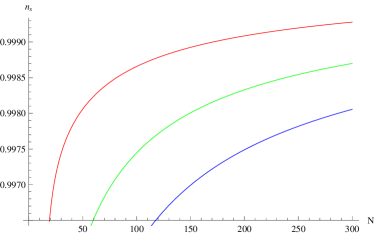
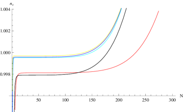
Figure 2: (left) $n_{s}$ versus $N$ for $A=8.225\times 10^{2},~{}\alpha=0.775,~{}\omega=-0.8,~{}\lambda=10$ (red), $50$ (green), $70$ (blue), $k=1$ (right) graph for $A=2.635\times 10^{2},~{}\alpha=0.81,~{}\omega=-1.5,~{}\lambda=10$ (red), $50$ (zinc), $70$ (purple); $A=8.407\times 10^{2},~{}\alpha=0.85,~{}\omega=-1.7,~{}\lambda=10$ (black), $50$ (blue), $70$ (yellow) in logamediate scenario.

$$n_{s}-1 = \left(\frac{3\lambda-2(\lambda-1)(\alpha+(1+\alpha)\psi)-2}{A\lambda}\right)\varepsilon^{\frac{3\lambda-2(\lambda-1)(\alpha+(1+\alpha)\psi)-2}{\lambda}}$$

$$+ \frac{2(\alpha+(1+\alpha)\psi-1)}{A\lambda}-\psi\left[\frac{A}{1+\omega}\left(\frac{\kappa}{3}\right)^{1+\alpha}(A\lambda)^{-2(1+\alpha)}\varepsilon^{\frac{-2(1+\alpha)}{\lambda}}\right.$$

$$\times \left.\exp\left[\frac{2\varepsilon(1+\alpha)}{\lambda}\right]\right]\left[\varepsilon^{-1}-1\right]\left[1-\frac{A}{1+\omega}\left(\frac{\kappa}{3}\right)^{1+\alpha}(A\lambda)^{-2(1+\alpha)}\varepsilon^{\frac{-2(1+\alpha)}{\lambda}}\right.$$

$$\times \left.\exp\left[\frac{2\varepsilon(1+\alpha)}{\lambda}\right]\right]^{-1}.$$

The graphical behavior of $n_{s}$ versus $N$ for different values of the model parameters is shown in Figure 2. The left graph shows that spectral index is an increasing function of $N$ which confirms the compatibility of the model with recent observations. In the right graph, zinc, yellow and blue curves correspond to $N=0$ for $n_{s}\leq 1$. Consequently, for all choices of free parameters, the model remains consistent with WMAP7 data. The tensor-scalar ratio becomes

$$r(N) = \frac{16(1-\lambda)}{A\lambda}\left(\frac{\kappa(A\lambda)^{2}}{3}\right)^{(\alpha+(1+\alpha)\psi)}\varepsilon^{\frac{1-2\lambda+2(\alpha+(1+\alpha)\psi)(\lambda-1)}{\lambda}}\exp\left[\varepsilon\left(\frac{1}{\lambda}-\frac{2}{\lambda}\alpha\right.\right.$$

$$+ \left.\left.(1+\alpha)\psi\right)\right]\left[1-\frac{A}{1+\omega}\left(\frac{\kappa}{3}\right)^{1+\alpha}(A\lambda)^{-2(1+\alpha)}\varepsilon^{\frac{-2(1+\alpha)}{\lambda}}\exp\left[\frac{2(1+\alpha)}{\lambda}\varepsilon\right]\right]^{\psi}.$$

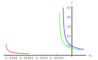
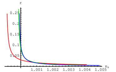
Figure 3: Tensor-scalar ratio versus $n_{s}$ in logamediate scenario.

During logamediate scenario, Figures 3 and 4 show similar decreasing behavior for all possible choices of the model parameters. In all cases, we cannot have $n_{s}=0.96$ in the allowed range of $r\leq 0.36$ which is compatible with WMAP7 data.

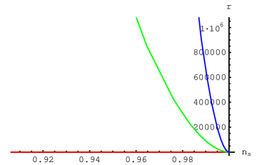
Figure 4: Tensor-scalar ratio versus $n_{s}$ in logamediate scenario.

3.2 Tachyon Scalar Field

In this section, we discuss the intermediate and logamediate inflationary scenarios in the presence of tachyon scalar field.

3.2.1 Intermediate Inflation

The solution of tachyon field during intermediate scenario is given by Eq.(10)

$$\phi(t)=\left[\frac{2(1-f)}{3(Af)(1+\omega)}\right]^{\frac{1}{2}}\left[\frac{A}{(1+\omega)\left(\frac{3(Af)^{2}}{\kappa}\right)^{1+\alpha}\chi}\right]t^{\frac{\chi}{2}},$$

which gives

$$t=\left[\phi\left[\frac{3(Af)(1+\omega)}{2(1-f)}\right]^{\frac{1}{2}}\left[\frac{(1+\omega)\left(\frac{3(Af)^{2}}{\kappa}\right)^{1+\alpha}\chi}{A}\right]\right]^{\frac{2}{\chi}},$$ (26)

where $\chi=f+2\alpha(f-1)-4(1+\alpha)(f-1)$. The scalar and tensor perturbed parameters in terms of $N$ are

$$\mathcal{P_{R}} = \left(\frac{\kappa}{3}\right)^{\alpha}\left(\frac{\kappa}{8\pi^{2}}\right)\frac{(Af)^{3-2\alpha}}{(1-f)}(1+\omega)^{\frac{1}{2}}\mu^{\frac{(f-1)(3-2\alpha)}{f}}\left[\left(\frac{3(Af)^{2}}{\kappa}\right)^{(1+\alpha)}\mu^{\frac{(f-1)(1+\alpha)}{f}}\right.$$

$$- \left.\frac{A}{1+\omega}\right]^{-\psi}\left[1+\left(\frac{2}{\kappa}\right)\left(\frac{3}{\kappa}\right)^{\alpha}(Af)^{2\alpha+1}(f-1)\mu^{\frac{(f-1)(1+2\alpha)}{f}}\left[\left(\frac{3(Af)^{2}}{\kappa}\right)^{1+\alpha}\right.\right.$$

$$\times \left.\left.\mu^{\frac{(f-1)(1+\alpha)}{f}}-\frac{A}{1+\omega}\right]^{-1}\right]^{-\frac{1}{2}},\quad\mathcal{P}_{g}=\left(\frac{2\kappa}{\pi^{2}}\right)(Af)^{2}\mu^{\frac{2(f-1)}{f}}.$$

The corresponding scalar spectral index is

$$n_{s}-1 = \frac{(1-f)(3-2\alpha)}{Af}\mu^{-1}-\left(\frac{3}{\kappa}\right)^{1+\alpha}(1+\alpha)(f-1)(Af)^{1+2\alpha}\mu^{\frac{(f-1)(1+\alpha)}{f}-1}$$

$$\times \left[\mu^{\frac{(f-1)(1+\alpha)}{f}}\left(\frac{3(Af)^{2}}{\kappa}\right)^{1+\alpha}-\frac{A}{1+\omega}\right]^{-1}-\frac{1}{2}\left[1+\left(\frac{2}{\kappa}\right)\left(\frac{3}{\kappa}\right)^{\alpha}(f-1)\right.$$

$$\times \left.(Af)^{1+2\alpha}\mu^{\frac{(f-1)(1+2\alpha)}{f}}\left[\left(\frac{3(Af)^{2}}{\kappa}\right)^{1+\alpha}\mu^{\frac{(f-1)(1+\alpha)}{f}}\frac{A}{1+\omega}\right]^{-1}\right]^{-1}$$

$$- \left[\left(\frac{2}{\kappa}\right)\left(\frac{3(Af)^{2}}{\kappa}\right)^{\alpha}(f-1)^{2}(1+2\alpha)\mu^{\frac{2\alpha(f-1)-1}{f}}\left[\left(\frac{3}{\kappa}\right)^{1+\alpha}(Af)^{2(1+\alpha)}\mu^{\frac{(f-1)(1+\alpha)}{f}}\right.\right.$$ (27)

$$- \left.\left.\frac{A}{1+\omega}\right]^{-1}\left(\frac{2}{\kappa}\right)\left(\frac{3}{\kappa}\right)^{1+2\alpha}(Af)^{2(1+2\alpha)}(1-f)^{2}(1+\alpha)\mu^{\frac{(f-1)(2+3\alpha)-f}{f}}\right.$$

$$\times \left.\left[\left(\frac{3}{\kappa}\right)^{1+\alpha}(Af)^{2(1+\alpha)}\mu^{\frac{(f-1)(1+\alpha)}{f}}-\frac{A}{1+\omega}\right]^{-2}\right].$$

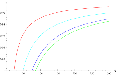
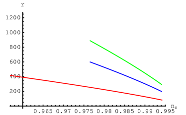
Figure 5: (left) $n_{s}$ versus $N$ (right) tensor-scalar ratio versus $n_{s}$ in intermediate scenario.

From $\mathcal{P_{R}}$ and $\mathcal{P}_{g}$, we find tensor-scalar ratio as

$$r(N) = 16\left(\frac{3}{\kappa}\right)^{\alpha}(1+\omega)^{-\frac{1}{2}}(1-f)(Af)^{2\alpha-1}\mu^{\frac{(f-1)(2\alpha-1)}{f}}\left[\left(\frac{3}{\kappa}\right)^{1+\alpha}(Af)^{2(1+\alpha)}\right.$$

$$\times \left.\mu^{\frac{(f-1)(1+\alpha)}{f}}-\frac{A}{1+\omega}\right]^{\psi}\left[1+\left(\frac{2}{\kappa}\right)\left(\frac{3}{\kappa}\right)^{\alpha}(f-1)(Af)^{1+2\alpha}\mu^{\frac{(f-1)(1+2\alpha)}{f}}\right.$$

$$\times \left.\left[\left(\frac{3}{\kappa}\right)^{1+\alpha}(Af)^{2(1+\alpha)}\mu^{\frac{(f-1)(1+\alpha)}{f}}-\frac{A}{1+\omega}\right]^{-1}\right]^{\frac{1}{2}}.$$

The left graph of Figure 5 represents increasing behavior for all four choices of the parameters. In this case, the value of $n_{s}=0.96$ corresponds to $N\approx 20$ (red), $50$ (zinc), $70$ (blue), $90$ (green). Thus the GCCG inflationary intermediate model with tachyon field is compatible with WMAP7 data. While the right graph of Figure 5 shows that the curves in $r-n_{s}$ plane are decreasing which indicate incompatibility of this model with recent observations. The physically acceptable range of the tensor-scalar ratio is not attained at $n_{s}=0.96$ during intermediate scenario using tachyon field.

3.2.2 Logamediate Inflation

Using logamediate scale factor in Eq.(10), we have

$$\phi(t)-\phi(t_{0})=\left[\left(\frac{2}{\kappa}\right)\left(\frac{3}{\kappa}\right)^{\alpha}\frac{\lambda-1}{1+\omega}(A\lambda)^{1+2\alpha}\right]^{\frac{1}{2}}\Xi(t),$$ (28)

which provides $t$ in terms of $\phi$ (by assuming $\phi(t_{0})=0$) as

$$t=\Xi^{-1}\left[\left[\left(\frac{2}{\kappa}\right)\left(\frac{3}{\kappa}\right)^{\alpha}\frac{\lambda-1}{1+\omega}(A\lambda)^{1+2\alpha}\right]^{-\frac{1}{2}}\phi\right].$$

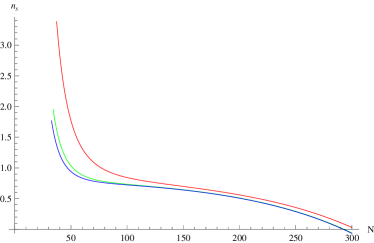
Figure 6: $n_{s}$ versus $N$ in logamediate scenario.

The scalar as well as tensor power spectra can be expressed as

$$\mathcal{P_{R}} = \left(\frac{\kappa}{3}\right)^{\alpha}\left(\frac{\kappa}{8\pi^{2}}\right)\frac{(1+\omega)^{\frac{1}{2}}}{1-\lambda}(A\lambda)^{3-2\alpha}\varepsilon^{\frac{3\lambda-2\alpha(\lambda-1)-2}{\lambda}}\exp\left[\frac{2\varepsilon(\alpha-1)}{\lambda}\right]\left[\left(\frac{3}{\kappa}\right)^{1+\alpha}\right.$$

$$\times \left.(A\lambda)^{2(1+\alpha)}\varepsilon^{\frac{2(1+\alpha)(\lambda-1)}{\lambda}}\exp\left[\frac{-2\varepsilon(1+\alpha)}{\lambda}\right]-\frac{A}{1+\omega}\right]^{1-\psi},$$

$$\mathcal{P}_{g} = \left(\frac{2\kappa}{\pi^{2}}\right)(A\lambda)^{2}\varepsilon^{\frac{2(\lambda-1)}{\lambda}}\exp\left[-\frac{2\varepsilon}{\lambda}\right].$$

The scalar spectral index has the form

$$n_{s}-1 = \left(\frac{3\lambda-2\alpha(\lambda-1)-2}{A\lambda}\right)\varepsilon^{-1}+\frac{2(\alpha-1)}{A\lambda}+2(1-\psi)(1+\alpha)(\lambda-1)\left(\frac{3}{\kappa}\right)^{1+\alpha}$$

$$\times (A\lambda)^{2\alpha-1}\left[\left(\frac{3}{\kappa}\right)^{1+\alpha}(A\lambda)^{2(1+\alpha)}\varepsilon^{\frac{2(1+\alpha)(\lambda-1)}{\lambda}}\exp\left[\frac{-2(1+\alpha)}{\lambda}\varepsilon\right]-\frac{A}{1+\omega}\right]^{-1}$$

$$\times \varepsilon^{\frac{2(1+\alpha)(\lambda-1)}{\lambda}-1}+\frac{1}{1-\lambda}\exp\left[\frac{-2(1+\alpha)}{\lambda}\left[\frac{N}{A}+(A\lambda)^{\frac{\lambda}{1-\lambda}}\right]\right].$$

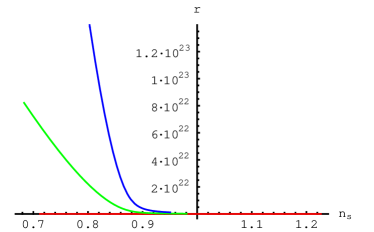
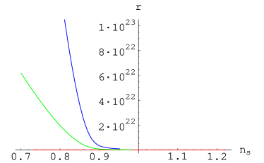
Figure 7: The left graph of tensor-scalar ratio versus $n_{s}$ in logamediate scenario.

The left and right graphs of Figure 6 show opposite behavior to each other for different values of $\lambda$. In the left graph, when $\lambda$ increases, $n_{s}$ decreases as $N$ increases for all three curves and the constrained $n_{s}=0.96$ corresponds to $N\approx 50$ for green and blue curves while $N\approx 100$ for red one. The right graph shows increasing trajectories and $n_{s}=0.96$ lies in the region $N<50$ for all choices of the model parameters. The tensor-scalar ratio is

$$r(N) = -16\left(\frac{3}{\kappa}\right)^{1+\alpha}\frac{(\lambda-1)}{(\omega+1)^{\frac{1}{2}}}(A\lambda)^{2\alpha-1}\varepsilon^{\frac{2\alpha(\lambda-1)-\lambda}{\lambda}}\exp\left[\frac{-2\varepsilon(\alpha+4)}{\lambda}\right]$$

$$\times \left[\left(\frac{3(A\lambda)^{2}}{\kappa}\right)^{1+\alpha}\varepsilon^{\frac{2(1+\alpha)(\lambda-1)}{\lambda}}\exp\left[\frac{-2\varepsilon(1+\alpha)}{\lambda}\right]-\frac{A}{1+\omega}\right]^{\psi+1}.$$

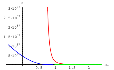
Figure 8: Tensor-scalar ratio versus $n_{s}$ in logamediate scenario.

Both graphs of Figure 7 show similar behavior as increasing $\lambda$ leads to increasing $r-n_{s}$ trajectories. The red curve in both graphs indicates that $r=0$ for $n_{s}=0.96$ which is incompatible according to WMAP7 data. Figure 8 shows decreasing behavior with increasing $\lambda$. In this case, $n_{s}=0.96$ corresponds to $r=0$ for $\lambda=50,~{}70$ while red curve $(\lambda=10)$ does not lie in the region $r<0.36$.

4 Concluding Remarks

In this paper, we have discussed GCCG inflationary universe model for flat FRW geometry during intermediate as well as logamediate scenarios. The standard and tachyon scalar fields are considered as matter content of this universe. In order to study Chaplygin inspired inflation, we have modified the first Friedmann equation by applying slow-roll approximation and found solutions of scalar fields as well as their corresponding potentials. We have also evaluated slow-roll parameters, number of e-folds, scalar and tensor power spectra, scalar index and finally the important parameter tensor-scalar ratio which is constrained by WMAP7 data. We have checked the physical compatibility of our model with WMAP7 results, i.e., the standard value $n_{S}=0.96$ must be found in the region $r<0.36$. The trajectories $N-n_{S}$ and $r-n_{S}$ are plotted to explore the behavior of these parameters in each case.

By constraining $0.96\leq n_{s}\leq 1.002$ and $\mathcal{P_{R}}(k_{0}=0.002Mpc^{-1})=(2.445\pm 0.096)\times 10^{-9}$, according to the observations of WMAP7, we obtain values of the model parameter as $A=8.225\times 10^{2},~{}2.635\times 10^{2},~{}8.407\times 10^{2}$ for $\alpha=0.775,~{}0.81,~{}0.85,~{}\omega=-0.8,-1.5,-1.7,~{}g=\frac{1}{2},~{}\kappa=1$ from Eq.(21). Using these values, we plot the graph of $N$ and $r$ versus $n_{s}$ in intermediate and logamediate scenarios. The left graph of Figure 1 shows that $n_{s}=0.96$ corresponds to $N=20$ for all possible choices of the model parameters during intermediate era. While right panel of Figure 1 shows that none of the case is compatible with WMAP7 data as the observed value $0.96\leq n_{s}\leq 1$ does not lie in the region $r\leq 0.36$. The graphical analysis of intermediate era represents incompatibility of the considered inflationary universe model for standard scalar field with WMAP7 data. During logamediate era, the left and right panels of Figure 2 represent similar increasing trajectories of $N-n_{s}$ with the increase and decrease of model parameters $\lambda=10,~{}50,~{}70$, respectively. Thus the number of e-folds remains consistent with observational value of $n_{s}$ according to WMAP7 data. On the other hand, Figures 3 and 4 show similar decreasing behavior for all possible choices of the model parameters. The graphical analysis of this observational parameter of interest $r$ versus $n_{s}$ shows violation of the observed value of WMAP7 (as $n_{s}=0.96$ does not correspond to $r\leq 0.36$). Thus we conclude that the GCCG inflationary universe model with a standard scalar field remains incompatible with observational data of WMAP7.

For tachyon field of the inflationary universe, left plot of Figure 5 represents increasing behavior of $N$ with respect to $n_{s}$ for all four choices of the parameters. In this case, $N$ remains consistent with observational value of $n_{s}$ as for standard scalar field. While right graph of Figure 5 shows incompatibility of this inflationary model with recent observations of WMAP7 by decreasing $r-n_{s}$ trajectories. In logamediate era, the left and right graphs of Figure 6 are opposite in nature for different values of $\lambda$. In the left panel, $n_{s}-N$ decreases with the increase of $\lambda$ while right panel shows increasing trajectories and $n_{s}=0.96$ lies in the region $N<50$ for all choices of the model parameters. Figures 7 and 8 show similar behavior as obtained for standard scalar field during logamediate era, i.e., increasing $\lambda$ leads to decreasing $r-n_{s}$ trajectories. In this case, the red curve in both graphs matches (i.e., for $n_{s}=0.96,~{}r=0$) which is not physical value of $r$ according to WMAP7 data. We conclude that the inflationary universe model remains incompatible with WMAP7 data for standard and tachyon scalar fields both in intermediate and logamediate scenarios. Thus accelerating expansion of the universe cannot be achieved by using GCCG inflationary universe model in both intermediate and logamediate regimes.

It is worth mentioning here that all the results for intermediate regime with standard and tachyon scalar fields reduce to [24]. Our results for this model support the results of [32] that this model is less effective as compared to MCG and other DE models.

Acknowledgment

We would like to thank the Higher Education Commission, Islamabad, Pakistan for its financial support through the Indigenous Ph.D. Fellowship for 5K Scholars, Phase-II, Batch-I.

References

- [1] Perlmutter, S. et al.: Nature 391(1998)51; Riess, A.G. et al.: Astron. J. 116(1998)1009.
- [2] Ratra, B. and Peebles, P.J.E.: Phys. Rev. D 37(1998)3406; Chiba, T., Okabe, T. and Yamaguchi, M.: Phys. Rev. D 62(2000)023511; Padmanabhan, T.: Phys. Rev. D 66(2002)021301; Guo, Z.K. et al.: Phys. Lett. B 608(2005)177.
- [3] Gorini, V., Kamenshchik, A. and Moschella, U.: Phys. Rev. D 67(2003)063509; Hu, B. and Ling, Y.: Phys. Rev. D 73(2006)123510; Setare, M.R.: J. Cosmol. Astropart. Phys. 0701(2007)023.
- [4] Zimdahl, W. and Fabris, J.C.: Class. Quantum Grav. 22(2005)4311.
- [5] Bazeia, D.: Phys. Rev. D 59(1999)085007.
- [6] Debnath, U., Banerjee, A. and Chakraborty, S.: Class. Quantum Grav. 21(2004)5609.
- [7] González-Diaz, P.F.: Phys. Rev. D 68(2003)021303.
- [8] Kamenshchik, A., Moschella, U. and Pasquier, V.: Phys. Lett. B 511(2001)265.
- [9] Sen, A.: Mod. Phys. Lett. A 17(2002)1797.
- [10] Sami, M., Chingangbam, P. and Qureshi, T.: Phys. Rev. D 66(2002)043530.
- [11] Gibbons, G.W.: Phys. Lett. B 537(2002)1.
- [12] Bento, M.C., Bertolami, O. and Sen, A.: Phys. Rev. D 66(2002)043507.
- [13] Dev, A., Alcaniz, J.S. and Jain, D.: Phys. Rev. D 67(2003)023515; González-Diaz, P.F.: Phys. Lett. B 562(2003)1; Kremer, G.M.: Gen. Relativ. Gravit. 35(2003)1459; Bean, R. and Dore, O.: Phys. Rev. D 68(2003)023515; Chimento, L.P.: Phys. Rev. D 69 (2004)123517.
- [14] Bertolami, O. and Duvvuri, V.: Phys. Lett. B 640(2006)121.
- [15] del Campo, S. and Herrera, R.: Phys. Lett. B 660(2008)282; ibid. 665(2008)100.
- [16] Monerat, G.A. et al.: Phys. Rev. D 76(2007)024017.
- [17] Starobinsky, A.A.: Phys. Lett. B 91(1980)99; Guth, A.: Phys. Rev. D 23(1981)347.
- [18] Gold, B. et al.: Astrophys. J. Suppl. 192(2011)15.
- [19] Yokoyama, J. and Maeda, K.: Phys. Lett. B 207(1988)31.
- [20] Setare, M.R. and Kamali, V.: Gen. Relativ. Gravit. 46(2014)1642.
- [21] Ferreira, P.G. and Joyce, M.: Phys. Rev. D 58(1998)023503; Barrow, J.D. and Nunes, N.J.: Phys. Rev. D 76(2007)043501.
- [22] Setare, M.R. and Kamali, V.: arXiv:1309.2452.
- [23] Sharif, M. and Saleem, R.: Eur. Phys. J. C 74(2014)2738.
- [24] Herrera, R., Olivares, M. and Videla, N.: Eur. Phys. J. C 73(2013)2295.
- [25] Barrow, J.D. and Liddle, A.R.: Phys. Rev. D 47(1993)5219; Starobin- sky, A.A.: J. Exp. Theor. Phys. Lett. 82(2005)169; del Campo, S., Her- rera, R., Saavedra, J., Campuzano, C. and Rojas, E.: Phys. Rev. D 80(2009)123531; Herrera, R. and Videla, N.: Eur. Phys. J. C 67(2010)499.
- [26] Martin, J. and Schwarz, D.J.: Phys. Rev. D 57(1998)3302.
- [27] Zarrouki, R. and Bennai, M.: Phys. Rev. D 82(2010)123506.
- [28] Liddle, A. and Lyth, D.: Cosmological Inflation and Large-Scale Structure, (Cambridge University Press, 2000).
- [29] Garousi, M.R., Sami, M., Tsujikawa, S.: Phys. Rev. D 70(2004)043536.
- [30] Sanyal, A.K.: Phys. Lett. B 645(2007)1.
- [31] Barrow, J.D.: Class. Quantum Grav. 13(1996)2965.
- [32] Rudra, P.: Astrophys. Space Sci. 342(2012)579.