Depinning of stiff directed lines in random media

Abstract

Driven elastic manifolds in random media exhibit a depinning transition to a state with non-vanishing velocity at a critical driving force. We study the depinning of stiff directed lines, which are governed by a bending rigidity rather than line tension. Their equation of motion is the (quenched) Herring-Mullins equation, which also describes surface growth governed by surface diffusion. Stiff directed lines are particularly interesting as there is a localization transition in the static problem at a finite temperature and the commonly exploited time ordering of states by means of Middleton’s theorems (A. Middleton, Phys. Rev. Lett. 68, 670 (1992)) is not applicable. We employ analytical arguments and numerical simulations to determine the critical exponents and compare our findings with previous works and functional renormalization group results, which we extend to the different line elasticity. We see evidence for two distinct correlation length exponents.

I Introduction

Elastic manifolds in random media are one of the most important model systems in the statistical physics of disordered systems, which exhibit disorder-dominated pinned phases with many features common to glassy systems Halpin-Healy and Zhang (1995); Blatter et al. (1994). Likewise, the depinning of an elastic manifold from a disorder potential under the action of a driving force is a paradigm for the non-equilibrium dynamical behavior of disordered systems capturing the avalanche dynamics of many complex systems if they are driven through a complex energy landscape Paczuski et al. (1996).

In particular, the problem of a directed line (DL) or directed polymer (i.e., an elastic manifold in $1+1$ dimensions) in a random potential and driven by a force has been subject of extensive study Feigel’man (1983); Sneddon et al. (1982); Middleton (1992); Chauve et al. (2000); Le Doussal et al. (2002); Duemmer and Krauth (2005); Le Doussal and Wiese (2007); Middleton et al. (2007); Rosso et al. (2007); Ferrero et al. (2013a). At zero temperature, there is a threshold force, at which the manifold changes from a localized state with vanishing mean velocity to a moving state with a non-zero mean velocity.

The depinning transition has been treated within the framework of classical critical phenomena by functional renormalization group techniques starting from the more general problem of depinning of $D$-dimensional elastic interfaces (with $D=1$ corresponding to lines). In $D=4-\epsilon$ dimensions, “critical” exponents at depinning can be calculated by functional renormalization using dimensional regularization in an $\epsilon$-expansion Narayan and Fisher (1992a, b); Nattermann et al. (1992).

At finite temperature, there is experimental evidence for a creep motion at any non-vanishing driving forces which can be understood qualitatively as thermally activated crossing of energy barriers which result from an interplay of both elastic energies of the line and the disorder potential.

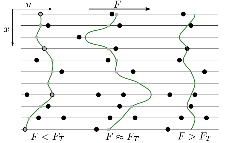
Figure 1: Schematic figure of typical SDL configurations below, at, and above the depinning transition (from left to right) in random-potential (RB) disorder. The black circles represent especially favorable locations within the random potential. Segments of the line that are currently not moving are marked with gray squares.

The energy of DLs such as flux lines, domain walls, wetting fronts is proportional to their length; therefore, the elastic properties of directed lines are governed by their line tension, which favors the straight configuration of shortest length. Here, we concentrate on stiff directed lines (SDLs), whose elastic energy is given by the curvature of the line and, thus, represents a bending energy. This gives rise to configurations which are locally curvature-free and straight but, in contrast to the DL, the straight segments of SDLs can assume any orientation even if this increases the total length of the line.

There are a number of applications and interesting general theoretical issues concerning SDLs in random media. The overdamped equation of motion of a SDL is the (fourth-order) Herring-Mullins linear diffusion equation Herring (1951); Mullins (1957), which also describes surface growth governed by surface diffusion. The depinning dynamics of the Herring-Mullins equation in quenched disorder has been subject of a number of prior studies Park and Kim (2000); Lee and Kim (2006); Liu et al. (2008); Song and Kim (2006), whose findings (e.g., an unphysically small roughness exponent) differ in part significantly from ours as we will point out below (see Sec. II.2). SDLs also describe semiflexible polymers with contour lengths smaller than their persistence length for bending fluctuations, such that the assumption of a directed line is not violated Kierfeld et al. (2006a). Our results can be applied to the depinning dynamics of semiflexible polymers such as DNA or cytoskeletal filaments like F-actin in a random environment, such as a porous medium, as long as the correlation length of the depinning transition is smaller than the persistence length. As in other semiflexible polymer phase transitions (such as adsorption) non-universal quantities such as the value of the depinning threshold itself will be governed by the bending elasticity. At the depinning transition, where the correlation length diverges, semiflexible polymers will exhibit a crossover to critical properties of effectively flexible lines (DLs) with a segment length set by the persistence length.

Moreover, static SDLs in a random potential feature a disorder-driven localization transition at finite temperatures already in $1+1$ dimensions Bundschuh and Lässig (2002); Boltz and Kierfeld (2012, 2013). Due to an interesting dimensional shift in the problem, an analogous transition occurs for DLs only in higher dimensions. In principle, this offers an opportunity to observe new phenomena arising from an interplay of depinning and delocalization for SDLs (the disorder used in Refs. Park and Kim (2000); Lee and Kim (2006); Liu et al. (2008); Song and Kim (2006) does not feature such a transition in the static problem). The localization transition at a finite temperature also offers the opportunity to test the usage of static quantities in the treatment of creep motion, because the SDL is not pinned by disorder above the critical temperature.

A lot of the progress for the depinning theory of DLs has been based on two basic theorems due to Middleton Middleton (1992), which essentially state that a forward moving DL can only move forward and will stop in a localized configuration, if such exists. This allows for an unambiguous time-ordering of a sequence of states. We will show that these theorems do not hold for the SDL, which can be seen as a consequence of the next-to-neighbor terms that are introduced by the bending elasticity.

The paper is organized as follows. We present the model and the relevant equations of motion in Sec. II, where we also comment on some equilibrium properties and previous work on the SDL. In Sec. III we present analytical results based on scaling arguments and functional renormalization group calculations. In Sec. IV we present numerical methods and results and, in Sec. V, we comment on the non-applicability of Middleton’s theorems for SDLs. We conclude with a summary of our results in Sec. VI.

II Model

A general approach to driven elastic manifolds starts from $1+D$ dimensional manifolds with an elastic energy

$$\mathcal{H}_{\text{el}} =\frac{1}{2}\int\mathrm{d}^{D}x\left(\partial^{a}_{x}u\right)^{2}\text{.}$$ (1)

As an external pulling force $F$ intrinsically couples to only one transversal displacement component $u$, there is no substantial gain in treating more than one transverse dimension, and we will restrict our analysis to this case. We assume that the manifold’s internal coordinates $x$ are bounded to the $D$-dimensional hypercube $[0,L]^{D}$ and call $L$ the system size (or length in $D=1$). We are mostly interested in the simplest case of lines with $D=1$. The order of the derivative $a$ distinguishes different kind of elasticities, $a=1$ is the directed line (DL) with tensional elasticity, and $a=2$ is the stiff directed line Boltz and Kierfeld (2012, 2013) (SDL) with bending elasticity.

The equilibrium statistics of the SDL and DL model are related as there is a mapping of the SDL to the DL model in higher transverse dimensions in problems with short-ranged potentials Bundschuh et al. (2000); Kierfeld and Lipowsky (2005). In an earlier work we extended this mapping between SDL and DL in short-ranged random potentials Boltz and Kierfeld (2012, 2013). In the context of polymers, the SDL model is often used as a weak-bending approximation to the so-called worm-like chain or Kratky-Porod model Harris and Hearst (1966); Kratky and Porod (1949), which is the basic model for inextensible semiflexible polymers, such as DNA, cytoskeletal filaments like F-actin, or polyelectrolytes. The weak-bending approximation is only applicable on length scales below the persistence length $L_{p}$, where tangent fluctuations $\overline{\langle(\partial_{x}u)^{2}\rangle}<1$ remain small. The persistence length contains thermal and disorder contributions as discussed in Refs. Boltz and Kierfeld (2012, 2013). Additionally, there is a relation of the SDL model to surface growth models, on which we will comment below.

In suitable units, the overdamped equation of an elastic line with an elastic energy $\mathcal{H}_{\text{el}}$ as in (1) can be written as

$$\frac{\partial u(x)}{\partial t} =-\frac{\delta\mathcal{H}_{\text{el}}}{\delta u(x)}+\eta(x,u)+F$$ (2)

at zero temperature. The first term on the right hand side represents the elastic forces as obtained from variation of the elastic energy (1). The force $F$ denotes a static, uniform pulling force, which tends to depin the line from the disordered medium, and $\eta(x,u)$ is a quenched force due to the disordered medium. For this quenched force we distinguish two cases in the following, random-field and random-potential disorder. For random-field (RF) disorder, $\eta(x,u)$ is a random variable with zero mean and short-ranged correlations

$$\overline{\eta(x,u)\eta(x^{\prime},u^{\prime})} \propto\delta(x-x^{\prime})\delta(u-u^{\prime})\quad\text{(RF),}$$ (3)

whereas for random-potential or random-bond (RB) disorder the force $\eta(x,u)=-\partial_{u}V(x,u)$ stems from a random potential $V(x,u)$, which features zero mean and short-ranged correlations. Hence, after a Fourier transformation in the transverse dimension, we can write

$$\overline{\eta(x,q)\eta(x^{\prime},q^{\prime})} \propto q^{2}\delta(x-x^{\prime})\delta(q+q^{\prime})\quad\text{(RB).}$$ (4)

Within this work we will mostly focus on random-potential (RB) disorder; in particular, all our numerical results in Sec. IV are for RB disorder. The analytical arguments in Sec. III, i.e., scaling relations and functional renormalization group results will be applied to both types of disorder.

If thermal fluctuations at temperature $T$ are included, an additional time-dependent white noise $\tau(x,t)$ with zero mean and correlations

$$\langle\tau(x,t)\tau(x^{\prime},t^{\prime})\rangle_{T} =2T\delta(x-x^{\prime})\delta(t-t^{\prime})$$ (5)

is added on the right hand side of eq. (2). We use $\langle X\rangle$ to denote averages over time, $[X]$ for spatial averages at a given time, $\overline{X}$ for the average over realizations of the quenched disorder and $\langle X\rangle_{T}$ for the average over realizations of the thermal noise. A subscript $c$ at an average denotes a cumulant.

At zero temperature, there is a finite threshold value $F_{T}$ at which the velocity

$$v(t) =\overline{[\dot{u}(x,t)]}$$ (6)

of a driven elastic manifold in a pinning potential becomes nonzero in the limit of very large times $t$

$$\langle v(t)\rangle \begin{cases}=0&F\leq F_{T}\\ >0&F>F_{T}\end{cases}\text{.}$$ (7)

The shape of the driven line and its dynamics are usually characterized by the roughness exponent $\zeta$ and the dynamical exponent $z$, which describe how the roughness or width of the line,

$$w^{2}(t) =\overline{[u(x,t)^{2}-[u(x,t)]^{2}]}=\overline{[u(x,t)^{2}]_{c}},$$ (8)

scales with the system size $L$ and the time $t$:

$$w^{2}(t)\sim\begin{cases}t^{2\zeta/z}&t\ll t_{L}\\ L^{2\zeta}&t\gg t_{L}\end{cases}$$ (9)

with the typical time scale

$$t_{L}\sim L^{z}.$$ (10)

SDLs with $a=2$ are closely related to surface growth models for molecular beam epitaxy (MBE) Barabási and Stanley (1995). In the presence of surface diffusion, MBE has been described by a (quenched) Herring-Mullins linear diffusion equation Herring (1951); Mullins (1957); Das Sarma et al. (1994); Racz and Plischke (1994) for a surface described by a height profile $u(x,t)$,

$$\frac{\partial u(x)}{\partial t} =-\nabla^{4}u(x)+\eta(x,u)+F\text{.}$$ (11)

In the Herring-Mullins limit, it is assumed that effects from a surface tension can be neglected as compared to surface diffusion effects. Surface tension would give rise to additional $\nabla^{2}u$-terms. In this context, the quantity $F$ describes the constant flux of particles onto the surface and $\eta(x,u)$ random fluctuations in the deposition process.

In suitable units, the Herring-Mullins equation (11) is equivalent to the overdamped equation of motion (2) of the SDL. Without external forces ($\eta=0$, $F=0$) the exponent $\zeta$ and $z$ take their thermal values $\zeta_{th}=3/2$ and $z_{th}=4$ Barabási and Stanley (1995). The observation of the “super-rough” $\zeta=3/2>1$ in tumor cells Brú et al. (1998) hints towards further experimental relevance of the Herring-Mullins equation.

For the DL with $a=1$, the equation of motion is the quenched Edwards-Wilkinson equation Edwards and Wilkinson (1982)

$$\frac{\partial u(x)}{\partial t} =\nabla^{2}u(x)+\eta(x,u)+F\text{,}$$ (12)

and the thermal exponents are $\zeta_{th}=1/2$ and $z_{th}=2$. Generally, the thermal exponents are given by $\zeta_{th}=a-\frac{D}{2}$ and $z_{th}=2a$.

II.1 Equilibrium properties

The equilibrium ($F=0$) problem of a SDL in a $1+1$-dimensional medium with RB disorder features a localization transition at a finite temperature $T_{c}$ as we pointed out in Refs. Boltz and Kierfeld (2012, 2013). The roughness exponent is $\zeta_{\text{eq,RB}}\approx 1.59>3/2$ in the disorder-dominated phase for $T<T_{c}$ and assumes the thermal value $\zeta=3/2$ for $T>T_{c}$. In contrast to the SDL, the DL with one transverse dimension is localized for all temperatures with a roughness exponent $\zeta_{\text{eq,RB}}=2/3$ Kardar (1987). This implies that the SDL in RB disorder offers the opportunity to study the dynamics of an unlocalized elastic manifold in disorder for $T>T_{c}$ and the interplay of the delocalization transition at $T=T_{c}$ and a depinning transition at $F=F_{T}$.

For RF disorder, functional renormalization group approaches Chauve et al. (2001); Le Doussal et al. (2004) using an expansion in $\varepsilon=4a-D$ around the upper critical dimension $D_{c}=4a$ give a static roughness exponent $\zeta_{\text{eq,RF}}=\varepsilon/3$ to at least two (and possibly all) orders in an expansion in $\varepsilon$ and in good agreement with numerical results both for the DL Belanger and Young (1991); Seppälä et al. (1998) and the SDL Lee et al. (2000). In a discrete model that directly implemented surface diffusion and was proposed to correspond to the undriven quenched Herring-Mullins equation a differing exponent $\zeta_{\text{eq,RF}}\approx 1.93$ was found for the SDL Park and Kim (2000).

The result $\zeta_{\text{eq,RF}}=\varepsilon/3$ is the simple scaling or “Flory” result, that follows from balancing the typical elastic energy of a line with displacement $u$, which scales as $E_{\text{el}}\sim L^{D}(u/L^{a})^{2}$, with the typical disorder energy $E_{\text{dis}}\sim\sqrt{L^{D}u}$ as the disorder energy is picked up at $L^{D}$ independent sites and its correlator decreases linearly in $u$ for large enough $u$ Fisher (1986). Similar arguments fail to reproduce the non-trivial RB roughness exponent, but can provide bounds to it as discussed in Refs. Boltz and Kierfeld (2012, 2013).

II.2 Previous work on the depinning of the quenched Herring-Mullins equation

There has been some previous work on the depinning of SDLs with RF disorder. From renormalization group analysis it is expected that the critical exponents of the depinning transition are universal for all disorders with shorter ranged correlations than RF (including RB), although a different scenario is possible in principle Le Doussal et al. (2002). For the DL the exponents do coincide for RF and RB disorder Ferrero et al. (2013a).

The roughness exponents previously found at the depinning of a SDL in RF disorder are $\zeta\approx 1.48-1.50$ and $\zeta=1.48$ and a dynamical exponent $z\approx 1.77-1.78$ Lee and Kim (2006); Liu et al. (2008). Furthermore, in a discrete model Song and Kim (2006) based on the quenched Herring-Mullins equation $\zeta=1.35$ and $z=1.60$ have been found at depinning. One obvious problem with these values for the roughness exponent $\zeta$ is that they are smaller than the thermal value $\zeta_{th}=3/2$, i.e., that disorder decreases the roughness of the line. We will comment below in more detail on similarities and differences in the findings of these studies to ours.

III Analytical results

III.1 Critical exponents and scaling relations

In order to describe the depinning of driven elastic lines in a random medium within the framework of classic critical phenomena Narayan and Fisher (1992a, b); Nattermann et al. (1992); Narayan and Fisher (1993), the roughness exponent $\zeta$ and dynamical exponent $z$ introduced in eq. (9) are not sufficient but one additional exponent related to the control parameter, the driving force $F$, is needed. In the vicinity of the depinning threshold $F_{T}$ we can introduce two exponents describing the “order parameter”, which is the velocity $v$ of the center of mass, and the correlation length $\xi$:

$$v \sim(F-F_{T})^{\beta}$$ (13)

$$\xi \sim(F-F_{T})^{-\nu}.$$ (14)

The correlation length $\xi$ gives the typical length of segments that rearrange during the avalanche-like motion close to the threshold; the typical time scale for this segment motion is $t_{\xi}\sim\xi^{z}$.

We can use one of these exponents, e.g. the correlation length exponent $\nu$, to obtain from the equilibrium scaling relation

$$w(t,L)=t^{\zeta/z}g(t/t_{L}^{z})$$ (15)

with a scaling function $g(x)$ (with $g(0)\approx 1$ and $g(x)\sim x^{-\zeta/z}$ for $x\gg 1$), which underlies eq. (9), a corresponding scaling relation close to depinning,

$$w(t,F)=t^{\zeta/z}g(t/t_{\xi}^{z})=t^{\zeta/z}f_{\pm}(t^{1/\nu z}(F-F_{T})),$$ (16)

with scaling functions $f_{\pm}(x)$ (for forces above (+) and below (-) the threshold and with $f_{\pm}(0)\approx 1$ and $f_{\pm}(x)\sim|x|^{-\zeta\nu}$ for $|x|\gg 1$).

There are two scaling laws relating the exponents $\beta$ and $\nu$ to the roughness exponent $\zeta$ and the dynamical exponent $z$ at the depinning transition. The first scaling law simply establishes a relation between $\beta$ and $\nu$ using that $v\sim w(t_{\xi})/t_{\xi}\sim\xi^{\zeta-z}$ (for $t\gg t_{\xi}$), which results in

$$\nu=\frac{\beta}{z-\zeta}.$$ (17)

This relation is valid independently of the form of the elastic energy, i.e., independent of $a$. As all exponents should be positive this also implies $z>\zeta$. The other relation comes from an additional tilt symmetry of the equation of motion Nattermann et al. (1992); Narayan and Fisher (1993), which leads to

$$\nu =\frac{1}{4-\zeta}$$ (18)

for the SDL ($a=2$) or, for general elasticity, to $\nu=(2a-\zeta)^{-1}$. The relations (17) and (18) should hold both for RF and RB disorder at depinning.

For the analysis of simulation data it is convenient to infer exponents from the short time scaling properties of the velocity, which follows from the scaling (16) and $v\sim w/t$:

$$v(t,F) \sim t^{\zeta/z-1}f_{\pm}(t^{1/\nu z}(F-F_{T}))$$

$$\sim t^{-\delta}f_{\pm}(t^{\gamma}(F-F_{T}))$$ (19)

where we introduce two auxiliary exponents

$$\gamma =1/\nu z$$ (20)

$$\delta =1-\zeta/z=\beta/\nu z=\beta\gamma,$$ (21)

for convenient data analysis [using the scaling relation (17) in eq. (21)].

The exponent values obtained previously in Ref. Lee and Kim (2006) are $\zeta\approx 1.50$ and $\nu\approx 1.01$ at the SDL depinning transition (for RF disorder). These values are problematic as they violate the scaling relation (18). One reason for this problem might be that the exponent $\zeta$ has been determined by direct measurement of the roughness $w(L)$ and its scaling for different system sizes $L$. However, such an approach is strongly influenced by the choice of the transverse system size (which should be $M\sim L^{\zeta}$) because the value for the critical force $F_{T}$ depends also on the transverse system size. As Ref. Lee and Kim (2006) contains two other independently measured exponents, namely $\delta$ and $\beta$ in our nomenclature, and scaling relations (17) and (18) imply $\zeta=4\beta(1-\delta)/(\delta+\beta(1-\delta))$. we can give a resulting “scaling” roughness exponent $\zeta_{\text{scaling}}\approx 2.4$, which strongly differs.

There is a another exponent that is often referred to as $\nu$ or $\nu_{\text{FS}}$ describing the scaling of the sample-to-sample fluctuations of the threshold force

$$\Delta F_{T}\sim L^{-1/\nu_{\text{FS}}}$$ (22)

in a system of finite size $L$. In general, $\nu$ and $\nu_{\text{FS}}$ do not have to coincide. For the DL, $\nu=\nu_{\text{FS}}\approx 4/3$ has been confirmed Duemmer and Krauth (2005); Bolech and Rosso (2004), whereas for the charge density wave problem (periodic potential), $\nu$ and $\nu_{\text{FS}}$ are distinct Middleton and Fisher (1991).

This might affect the scaling relations (17) and the auxiliary exponents $\gamma$ and $\delta$, see eqs. (20) and (21), which could read $\nu_{\text{FS}}=\beta/(z-\zeta)$, $\gamma=1/\nu_{\text{FS}}z$, and $\delta=\beta/\nu_{\text{FS}}z$. This happens if threshold force fluctuations by sample-to-sample disorder fluctuations on a scale $L$, $\Delta F_{T}\sim L^{-1/\nu_{\text{FS}}}$, are larger than the excess to the threshold force necessary to depin a segment of length $L$, $F-F_{T}\sim L^{-1/\nu}$, see eq. (14). Therefore, we expect $\nu<\nu_{\text{FS}}$ if $\nu$ and $\nu_{\text{FS}}$ are distinct.

Fluctuations in the depinning force $F_{T}$ origin from the fluctuations in the disorder. A finite manifold of size $L$ and width $w\sim L^{\zeta}$ occupying a volume $L^{D}w\sim L^{\zeta+D}$ should at least pick up the same free energy fluctuations as a summation of i.i.d. random numbers which are $\sim(\text{Vol.})^{\frac{1}{2}}$. This results in a general lower limit for the depinning force fluctuations Chayes et al. (1986)

$$\Delta F_{T}\geq c(\text{Vol.})^{-\frac{1}{2}}=\tilde{c}L^{-\frac{\zeta+D}{2}}$$ (23)

thus giving

$$\nu_{\text{FS}}\geq\frac{2}{\zeta+D}.$$ (24)

It has been argued that $\nu=\nu_{\text{FS}}$ for an elastic line as long as the line continuously “explores” new regions of the disorder Narayan and Fisher (1993). In this interpretation, distinct correlation length exponents $\nu$ and $\nu_{\text{FS}}$ for the charge density wave are a manifestation of the fact that the line “knows” the total potential at each point due to its periodicity. If $\nu=\nu_{\text{FS}}$ holds, the bound (24) is equivalent to a lower bound to the roughness exponent $\zeta$ at depinning,

$$\zeta\geq\varepsilon/3\quad\text{ if }\nu=\nu_{\text{FS}},$$ (25)

which is valid for all elastic energies of the form (1), i.e., for all $a$. The contraposition is equally important: if the roughness is less than $\varepsilon/3$, this implies that $\nu$ and $\nu_{\text{FS}}$ are distinct.

An upper bound to the roughness exponent comes from studying the line in the Larkin approximation with a constant ($u$-independent) random force acting on every segment of the line Larkin (1970); Blatter et al. (1994). The resulting Larkin roughness exponent is $\zeta_{\text{Larkin}}=\varepsilon/2$. As the line can gather unbound energy via large undulations in accordance with the force this represents an upper bound to the problem with finite potential range and, therefore,

$$\zeta\leq\varepsilon/2\text{,}$$ (26)

which holds for the roughness exponents $\zeta$ below, at, and above depinning.

III.2 Functional renormalization group

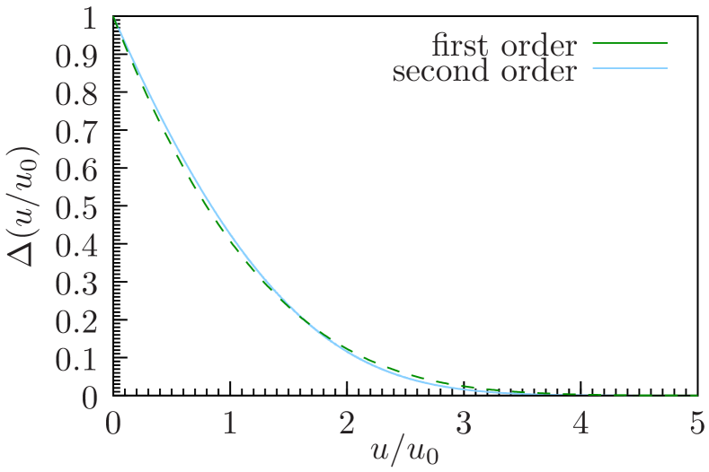
Figure 2: The fixed point solution to the functional renormalization group flow equation of Ref. Le Doussal et al. (2002) for the disorder correlator $\Delta(u)$. The length scale $u_{0}$ is determined via $\int\mathrm{d}u\Delta{(u/u_{0})}=1$. The two-loop solution corresponds to a roughness exponent given by eq. (27). The small deviations between first and second order give rise to distinct roughness exponents (29).

It has originally been suggested that the roughness exponent $\zeta$ at the threshold force $F=F_{T}$ is independent of the type of disorder (RB or RF) and coincides with the static roughness of the line in a medium with RF disorder $\zeta_{\text{eq,RF}}=\varepsilon/3$ to all orders of $\varepsilon$ Narayan and Fisher (1993). The discrepancy to numerical simulations Leschhorn (1993) has been solved by means of the two-loop functional renormalization group (FRG) Le Doussal et al. (2002), which gives for the roughness exponent at depinning both for RB and RF disorder

$$\zeta^{(2a)} =\frac{\varepsilon}{3}+\frac{X^{(2a)}\varepsilon^{2}}{27\sqrt{2}\gamma}+\mathcal{O}(\varepsilon^{3})$$ (27)

with the Euler-Mascheroni constant $\gamma$ and a constant $X^{(2a)}$ that depends on the form of the elastic energy, especially $X^{(2)}=1$ and $X^{(4)}=-1/6$. The FRG approach is based on a flow equation for the disorder force correlator $\Delta(u)$ defined by

$$\overline{\eta(x,u)\eta(x^{\prime},u^{\prime})} =\delta(x-x^{\prime})\Delta(u-u^{\prime})\text{.}$$ (28)

At two-loop order the FRG flow converges to the same fixed point disorder correlator (shown in Fig. 2) both for RB and RF disorder. Therefore, two-loop FRG predicts identical roughness exponents at depinning.

As $\varepsilon=4a-d$ is rather large for the SDL, the two-loop contribution is important. This can be seen in the significant deviation of the two naive results

$$\zeta_{\text{1-loop}}\approx 2.33~{}~{}\mbox{and}~{}~{}\zeta_{\text{2-loop}}\approx 1.94$$ (29)

using a direct evaluation of (27) (Padé approximants give values $\zeta_{\text{2-loop}}\approx 1.9432$ to $\zeta_{\text{2-loop}}\approx 1.999$). Thus the SDL roughness at depinning is expected to be above the static value for zero external force Boltz and Kierfeld (2012, 2013) $\zeta_{eq,RB}\approx 1.59$ for RB disorder, but below the static result $\zeta_{eq,RF}=7/3$ for RF disorder. We note that any extrapolation of the results in eq. (27) necessarily violates the bound (25), which holds if $\nu=\nu_{\text{FS}}$, as the negative two-loop contribution leads to $\zeta^{(4)}<\frac{\varepsilon}{3}$ for some finite $\varepsilon$. This is an indication for two distinct exponents $\nu$ and $\nu_{\text{FS}}$.

In Fig. 2 we show the numeric solution of the FRG fixed point for the disorder correlator $\Delta(u)$ verifying that eq. (27) does indeed correspond to the unique non-negative faster than algebraically decaying (convex in double logarithmic plot) solution. We followed the numerical procedure outlined in Refs. Le Doussal et al. (2002, 2004). The new second order contribution $y_{2}$ giving the two-loop contribution in the Ansatz $\Delta(u)=\varepsilon/3y_{1}(x)+\varepsilon^{2}/18y_{2}(x)+O(\varepsilon^{3})$ can be approximated by the Taylor series

$$y_{2}(x) \approx 0.190021u-0.1613u^{2}+3.37491\times 10^{-2}u^{3}$$

$$+3.21649\times 10^{-3}u^{4}-4.32055\times 10^{-4}u^{5}$$

$$-2.55032\times 10^{-4}u^{6}-4.7737\times 10^{-5}u^{7}$$

$$+1.0426\times 10^{-6}u^{8}+3.44412\times 10^{-6}u^{9}+O(u^{10})\text{.}$$ (30)

The FRG calculation presented in Ref. Le Doussal et al. (2002) is in principle also capable of determining the dynamical exponent $z$ and, thus, all exponents. However, to two loops this involves the evaluation (to leading order in $\varepsilon$) of the “correction to friction” which remains an open task. It is possible (details are given in appendix A) to find bounds for the value of the dynamical exponent $z$ in two-loop order

$$1.86\leq z_{\text{2-loop}}\leq 2.31\quad\text{.}$$ (31)

The exponents at one-loop order for the SDL are given in Table 1 together with the previous numerical findings.

exponent	$\zeta$	$z$	$\nu$	$\beta$	$\delta$
FRG	$7/3$	$22/9$	$3/5$	$1/15$	$1/22$
simulation Ref. Lee and Kim (2006)	$1.50$	$1.78$	$1.01$	$0.289(8)$	$0.160(5)$
simulation this paper	$2.00$	$2.15$	$0.50$	$0.29$	$0.07$

Table 1: Critical exponents at the SDL depinning transition determined via one-loop functional renormalization group (FRG) Le Doussal et al. (2002) and numerical simulation results from Ref. Lee and Kim (2006) and this work. The last line uses the numerical values for $\beta$ and $\delta$ and the scaling relations of Sec. III.1.

An interesting question in the FRG analysis is the stability of the fixed point solution. It has been argued Le Doussal et al. (2002); Narayan and Fisher (1993) that the two previously defined correlation length exponents coincide, that is $\nu=\nu_{\text{FS}}$, if the fixed point solution for the disorder correlator is stable. This is in agreement with the results for charge density waves (fixed point unstable Narayan and Fisher (1992a, b), $\nu\neq\nu_{\text{FS}}$ Middleton and Fisher (1991)) and the DL (fixed point presumably stable Le Doussal et al. (2002), $\nu\approx\nu_{\text{FS}}$ Duemmer and Krauth (2005)). We did not try to perform a full stability analysis, but we note that the simple argument of Ref. Le Doussal et al. (2002) for the instability of the fixed point for charge density waves might also hold for SDLs: after integrating the FRG flow equation from $u=0^{+}$ to $u=\infty$ it reads

$$-m\partial_{m}\int_{0}^{\infty}\!\Delta(u)\mathrm{d}u =(\varepsilon-3\zeta)\int_{0}^{\infty}\!\Delta(u)\mathrm{d}u-X^{(4)}\Delta^{\prime}(0^{+})^{3}\text{.}$$ (32)

The second contribution on the right hand side is negative because (to two loops)

$$\zeta^{(2a)} =\frac{1}{3}\varepsilon-\frac{X^{(2a)}\Delta^{\prime}(0^{+})^{3}}{3\int\Delta}=\frac{\varepsilon}{3}+\zeta^{(2a)}_{2}\varepsilon^{2}$$ (33)

and $\zeta^{(4)}_{2}<0$ (with the shorter notation $\int\Delta\equiv\int_{0}^{\infty}\mathrm{d}u\Delta(u)$). More importantly, this implies that $\zeta<\varepsilon/3$ and, thus, the FRG fixed point of $\int\Delta$ is unstable. The instability of the fixed point of eq. (32) leads to a flow of the form

$$\Delta_{m}(u)=\Delta^{*}(u)+cm^{-(\varepsilon-3\zeta)}$$ (34)

with $c=m_{0}^{\varepsilon-3\zeta}\int_{0}^{\infty}(\Delta_{m_{0}}(u)-\Delta^{*}(u))\mathrm{d}u$. Thus an additional constant ($u$-independent) contribution to the fixed point $\Delta^{*}(u)$ is generated, that grows as $m$ goes to zero if $\zeta<\varepsilon/3$. This means that to two-loop order a random force of the Larkin-type is generated. This random force generates the Larkin-like roughness

$$\zeta_{\text{Larkin}} =\varepsilon/2$$ (35)

which for the SDL with $\varepsilon=7$ implies a separate correlation length exponent

$$\nu_{\text{FS}} =\frac{1}{4-7/2}=2$$ (36)

according to the tilt-symmetry scaling relation (18).

III.3 Large force limit, crossover to single particle limit

For sufficiently large external forces we can generalize the perturbative arguments for DLs from Refs. Feigel’man (1983); Sneddon et al. (1982) to general elastic manifolds in $1+D$ Dimensions with an elastic energy of the form (1). Then, to second order in perturbation theory, the velocity of the center of mass of the line is

$$v \approx F-\text{const}\times F^{\frac{{D}-2a}{2a}}$$ (37)

Here we assumed a short-ranged random potential that is completely uncorrelated along the internal dimensions. For the problem at hand ($D=1$, $a=2$) this implies that the first correction at large forces should scale as

$$1-\frac{v}{F} \sim F^{-7/4}\text{.}$$ (38)

This is in agreement with our numerical results (see Sec. IV.4) for not too large forces. The asymptotic behavior for very large forces can be understood with the same perturbative reasoning that led to eq. (38), but neglecting the elastic forces and considering the effective single-particle (sp) equation $\frac{\partial u}{\partial t}=\eta(u)+F$. This leads to

$$v_{\text{sp}} =F-\text{const}\times F^{-1}R_{u}^{-3}$$ (39)

$$1-\frac{v_{\text{sp}}}{F} \sim F^{-2}\quad\text{.}$$ (40)

The crossover should happen, when the length scale $(\Delta_{u}/F)^{1/4}$ on which the elastic adjustments to the forced induced motion are relevant becomes significantly smaller than the lattice spacing $\Delta_{x}$. This is the length scale that corresponds to the time scale $\Delta_{u}/F$ for a moving line to get to the next “disorder site” for the free dynamic exponent $z_{0}=4$.

III.4 Finite Temperature

At finite temperatures $T>0$ there is a thermally activated motion, $\langle v\rangle>0$, for any driving force $F$. For the DL this dynamical phenomenon has successfully been described via the thermal activation over barriers that are determined from a static consideration as the motion is expected to be very slow for low temperatures and forces Chauve et al. (2000); Ioffe and Vinokur (1987); Nattermann et al. (1990). For forces $F<F_{T}$ below depinning this involves activation over large energy barriers (diverging in the limit $F\approx 0$) and results in so-called creep motion. As a result of thermal activation, the sharp depinning transition at $F=F_{T}$ is rounded. For forces $F>F_{T}$ above depinning the line moves with finite velocity and additional thermal activation has only little effect.

For the SDL, there is an additional complication because of the disorder-induced localization transition at a finite temperature $T_{c}$ Boltz and Kierfeld (2012, 2013). For temperatures $T<T_{c}$, we expect the SDL to behave qualitatively similar to a DL, i.e., to exhibit creep for $F<F_{T}$, thermal rounding of the depinning transition at $F=F_{T}$, and only minor modifications of the flow behavior for $F>F_{T}$. In order to derive the SDL creep law via a scaling argument, we consider the static equilibrium energy fluctuations, which scale as $E_{eq}\sim L^{\omega}$ with the (equilibrium) energy fluctuation exponent $\omega=D-2a+2\zeta_{eq}$. In a static framework, a depinning force $F$ simply tilts the energy landscape $U_{F}\sim FL^{D}w\sim FL^{D+\zeta_{eq}}\text{.}$ Balancing these two contributions to optimize the total barrier energy $E_{\text{barrier}}=E_{\text{eq}}-U_{F}$, one gets the energy of the effective barriers scaling as

$$E_{\text{barrier}} \sim F^{-\mu}$$ (41)

with the barrier exponent

$$\mu =\frac{D-2a+2\zeta_{eq}}{2a-\zeta_{eq}}=\frac{\omega}{2a-\zeta_{eq}}.$$ (42)

For lines with $D=1$, this gives $\mu=1/4$ for the DL and $\mu\approx 0.07$ for the SDL. The velocity follows from the Arrhenius law to be

$$v \sim\exp{\left[-\text{const}\times F^{-\mu}/T\right]}\text{.}$$ (43)

For the DL this has been confirmed experimentally Lemerle et al. (1998).

For temperatures $T>T_{c}$, on the other hand, the scenario is less clear. In the static problem, the SDL then depins already by thermal fluctuations. The roughness in the static problem is only larger than the thermal roughness, $\zeta_{eq}>\zeta_{th}$, for temperatures $T<T_{c}$ below the critical temperature Boltz and Kierfeld (2012, 2013). For $T>T_{c}$, the static SDL is thermally rough $\zeta_{th}=(4-D)/2$, and there are no macroscopic energy fluctuations. Assuming that the static equilibrium physics is indeed relevant for low driving forces (as in the derivation of the creep law), the conclusion could be that there are only finite energy barriers of characteristic size $E_{\text{barrier}}=C$, and the velocity is given by the so called thermally assisted flux flow (TAFF) Anderson and Kim (1964); Kes et al. (1989)

$$v_{\text{TAFF}} \propto F/T\exp{\left[-C/T\right]}\text{.}$$ (44)

The treatment within the FRG Chauve et al. (2000) suggests that (at least to one-loop order) the force-force correlator $\Delta$ is only affected by a finite temperature within the “thermal boundary layer” of width $\sim T$ (especially, there is only a “cusp” for $T=0$). Within this layer the line assumes the static roughness $\zeta_{eq}$, whereas on larger scales the dynamic roughness $\zeta>\zeta_{eq}$ becomes apparent (for finite $v>0$). Thus, the FRG seems to be in line with our previous reasoning, that is $\mu=0$ for $T>T_{c}$ and a TAFF-like velocity-force curve.

However, this comes with the substantial caveat that, to our knowledge, the FRG theory in its present form is not apt to describe the full temperature dependence and, in particular, the existence of a transition to thermal roughness (which should manifest itself in the emergence of a fixed point solution with roughness $\zeta_{th}$) at finite temperature. One basic difficulty is that a disorder-induced localization transition at a finite temperature $T_{c}$ does only occur for low dimensions $D<2a$, whereas the FRG uses an expansion around an upper critical dimension $D=4a$. In section IV.6, we will present numerical evidence that the thermal rounding of the depinning transition at the threshold force $F_{T}$ is very similar for DLs and SDLs. This surprising result suggests that the thermal depinning transition of the SDL in the absence of a driving force does not change the depinning by a driving force qualitatively.

The numerical determination of the barrier exponent $\mu$ is an unsolved problem even with algorithms specifically designed to capture the creep dynamics Kolton et al. (2009). The thermal rounding of the transition leads to a temperature dependent velocity at the (zero-temperature) threshold force, which, for the DL, has been found to follow a power-law

$$v_{F_{T}} =T^{\psi}.$$ (45)

It has been suggested that $\psi=\beta/(1+2\beta)$ Chauve et al. (2000); Tang and Stepanow (the perturbative argument in Ref. Chauve et al. (2000) is equally valid for the SDL). Numerically and experimentally a value $\psi\approx 0.15\approx\beta/(1+2\beta)$ ($\beta\approx 0.245$ Kolton et al. (2009)) has been found for the DL with RB disorder Bustingorry et al. (2008, 2012).

IV Numerical results

IV.1 Direct integration of the equation of motion

We make use of a recently presented implementation Ferrero et al. (2013a) for graphics processing units (GPUs). The high number of parallelly executed computations becomes very advantageous for large lengths, with an effective speedup of two orders of magnitude for the DL Ferrero et al. (2013a). As the different elastic force generates only little additional branching (the determination of the next-nearest neighbors with periodic boundaries), the GPU implementation is also favorable for SDLs.

Additionally, we implemented an equivalent simulation for CPUs. An Euler integration scheme is used for the benefit of computational simplicity.

In the numerical simulations we focus on random potential (RB) disorder (as opposed to Ref. Lee and Kim (2006)). The random potential is implemented by drawing random numbers from a normal distribution on a $L\times M$ lattice where $M$ is the transverse size of the system Rosso and Krauth (2002). Between the lattice points the potential is interpolated by periodic, cubic splines in $u$-direction. Disorder averages were performed over 1000 samples. Our system is periodic in $x$- and $u$-direction and the simulation starts with a flat line $u(x)\equiv 0$.

We set the lattice spacing in both directions equal to one, $\Delta_{x}=\Delta_{u}=1$, and approximate the fourth derivative by the central finite difference $\nabla^{(4)}u(x)\approx u(x-2)-4u(x-1)+6u(x)-4u(x+1)+u(x+2)$, which is of second order in space. A von-Neumann stability analysis shows that (without external forces) the Euler integration scheme becomes unstable for $\Delta t/\Delta_{x}^{2}>2^{-3}$. Throughout this work we used time steps $\Delta t\leq 2^{-6}$, unless stated differently.

As the width of the line can be influenced by various effects on different length scales, it can be difficult and error-prone to infer $\zeta$ directly from the line width $w$. Therefore, it is helpful to study the structure factor

$$S(q,t) =\overline{\lvert u(q,t)\rvert^{2}}\sim q^{-(2\zeta+1)}$$ (46)

where $u(q,t)$ is the Fourier transformation of $u(x,t)$. This assumes self-affinity of the line.

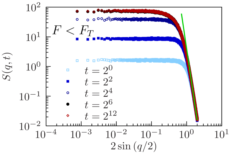
Figure 3: Disorder averaged structure factor $S(q,t)$ for a SDL with $F=1.00<F_{T}$ ($L=8192$, $M=16384$). The initial conditions (flat line) persist on long length scales and cross over to a regime with Larkin roughness ($\zeta_{\text{Larkin}}=7/2$, solid line) on short length scales. After adjustment to the disorder till about $t=2^{6}$ the conformation of the line does not change.

For sufficiently large $M$ the system is ergodic only above the threshold, when the line moves. Thus, for forces smaller than the threshold force (cp. Fig. 3) the line does not show the static roughness, but adjusts itself to the potential on short length scales (large wavenumbers) leading to Larkin roughness $\zeta_{\text{Larkin}}=7/2$, whereas the conformation on longer length scales (small wavenumbers) depends on the initial conditions. Here and in the following we plot the structure factor as a function of $2\sin{(q/2)}$ to correct for lattice artifacts.

IV.2 Short-time dynamics scaling

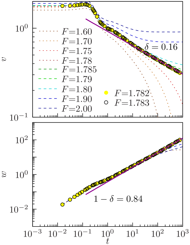
Figure 4: The disorder-averaged center-of-mass velocity $v(t)$ (top) and roughness $w(t)$ (bottom) in a system with $L=8192$, $M=16384$ for various forces and short times. Both quantities exhibit power-law regime consistent with $\delta=0.16$ at $F\approx 1.782-1.783$. For clarity we plotted the data for these data as full ($F=1.782$) and hollow ($F=1.783$) circles and used dashed ($F>1.783$) and dotted ($F<1.782$) lines for the rest (the key given in the upper figure holds for both). We note that the time-averaged roughness $\langle w(t)\rangle$ becomes maximal around $F\approx 1.782-1.783$.

Alike previous studies Kolton et al. (2006a); Ferrero et al. (2013a); Lee and Kim (2006) we employ short-time dynamics scaling to determine the critical exponents of the SDL at depinning. From eqs. (16) and (19) we know that, at $F=F_{T}$, velocity and line width scale as

$$v \sim t^{-\delta}\sim t^{-\beta/\nu z}$$ (47)

$$w \sim t^{1-\delta}\sim t^{\zeta/z}\quad\text{.}$$ (48)

These two observables contain the same information regarding the critical exponents. The behavior for forces near the threshold can be used to extract the exponent $\gamma=1/\nu z$ from rescaling the velocity according to eq. (19),

$$v(t,F)t^{\beta/\nu z}\sim f_{\pm}(t^{1/(\nu z)}(F-F_{T})).$$ (49)

However, with actual data it turns out to be difficult to extract precise and unambiguous exponents from this finite-size scaling like procedure. Additionally, the roughness exponent $\zeta$ becomes apparent in the structure factor $S(q,t)$ for wavenumbers below some $q_{t}\sim L_{t}^{-1}\sim t^{-1/z}$, see eq. (46).

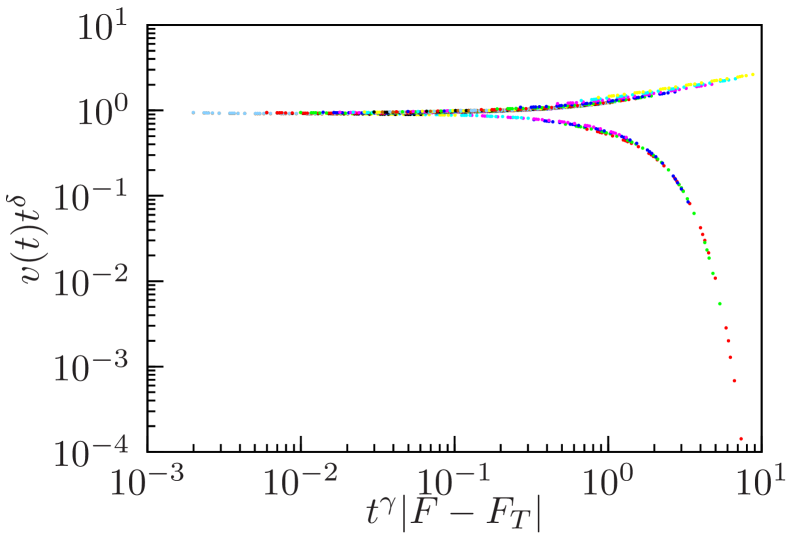
Figure 5: Scaling plot of the velocity for different forces and times using eq. (49). The upper branch contains forces $F>F_{T}$ and the lower one forces $F<F_{T}$. Parameters are as for Fig. 4, but we used more force values ($1<F<2$). As scaling is not expected to hold for small times, we only considered $t>10$. In agreement with Fig. 4, we used $F_{T}=1.7825$ and $\delta=0.16$. We see satisfying scaling for $\gamma\approx 0.55$, which coincides with the findings of Ref. Lee and Kim (2006).

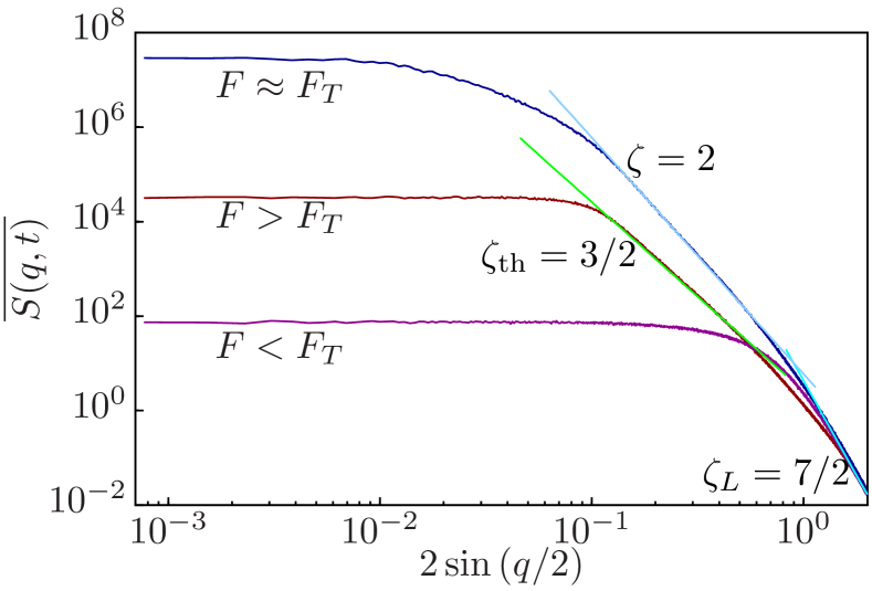
Figure 6: The disorder-averaged structure factor for a system with $L=8192$, $M=16384$ at time $t=4096$ at three different forces representing the three regimes: under-critical, critical and over-critical. Although configurations are not strictly self-affine (pure power-law behavior in the structure factor) there is a clear emergence of an exponent $\zeta=2$ around the threshold force. We identify this as the “critical” roughness exponent. As in Fig. 4, the system shows maximal roughness at the threshold.

In Ref. Lee and Kim (2006), $\delta\approx 0.16$ has been found from studying $v(t)$ and $w(t)$ for RF disorder. In Fig. 4 we obtain the same result for RB disorder. Additionally, we show in Fig. 5 that the data can be nicely matched using the scaling of eq. (49) and $\gamma\approx 0.56$ in agreement with Ref. Lee and Kim (2006). By definition of $\delta$ and $\gamma$, this implies $\beta=\delta/\gamma\approx 0.29$ and by means of scaling relations $\zeta\approx 2.4-2.5$ as we already pointed out in Sec. III.1. We do not find any evidence (at any force) in the structure factor supporting this roughness. We do observe the emergence of a new roughness exponent $\zeta\approx 2$ at higher forces as can be seen from Fig. 6. We consequently conclude that this is a more plausible location of the threshold force and that $\zeta\approx 2$ is indeed the threshold roughness exponent.

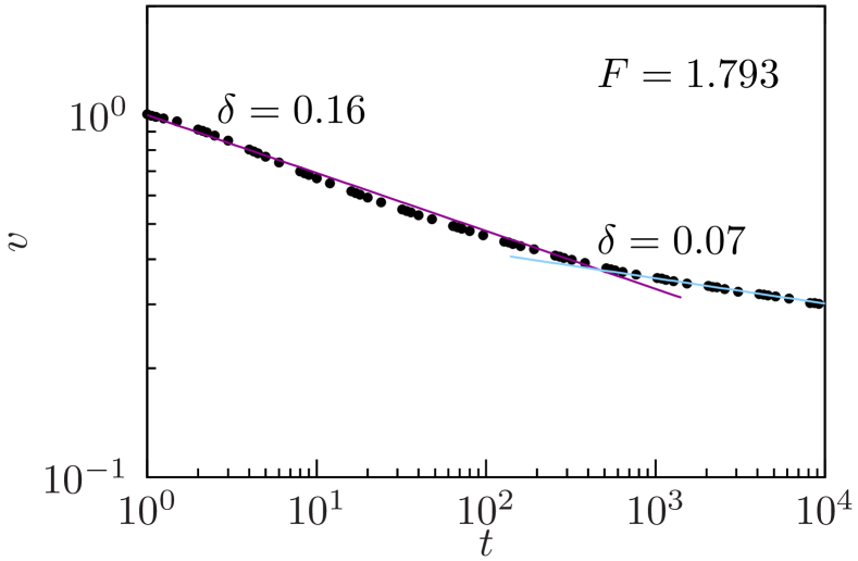
Figure 7: The disorder averaged center-of-mass velocity for $F=1.793$. The system parameters are as for Fig. 4, which suggested $F_{T}\approx 1.782-1.783$. The description by a power-law fits better in the “macroscopic” large time regime. Although we rather determined $F_{T}$ by demanding a consistent $\delta$ as in Figs. 4 and 5, we note that, for $F=1.793$, the second-power law fits particularly well.

The examination of $v(t)$ at higher forces and larger times reveals that the curves that do not saturate to a finite $v$ for large times ($F>F_{T}$) or go to zero ($F<F_{T}$) seem to consist of two power-law segments, where only the first one for smaller times is consistent with $\delta\approx 0.16$, see Fig. 7. This is analogous to the most recent findings for the DL in Ref. Ferrero et al. (2013a). In Fig. 7 we show $v(t)$ for $F=1.793$, which we believe to be close to the threshold force $F_{T}$ for the system size we use. As the exponent $\delta$ in the second power-law segment is rather close to zero and we have no independent method to determine $F_{T}$ (see also below in Sec. V) giving a precise value for $\delta$ is difficult. As the threshold roughness does not only influence the structure factor exactly at $F_{T}$, but also for deviating forces (given that the correlation length is still noticeable large), we think that we can rely on our value of $\zeta\approx 2$ even though we do not know $F_{T}$ precisely. Additionally, we will support the claim of a roughness exponent $\zeta\approx 2$ with an independent method below in Sec. IV.5. In Fig. 7 we show that $F_{T}=1.793$ is consistent with an exponent value $\delta\approx 0.07$ for larger times $t$, whereas $\delta\approx 0.16$ only at smaller times.

For $F_{T}=1.793$ we obtain, based on the numerical results $\delta\approx 0.07$ and $\zeta\approx 2.0$, the following set of exponents:

$$F_{T} \approx 1.793~{},~{}~{} \delta \approx 0.07~{},$$

$$\zeta \approx 2.0~{},~{}~{} z =\zeta/(1-\delta)\approx 2.15~{},$$

$$\nu =\frac{1}{4-\zeta}\approx 0.5~{},~{}~{} \beta =\nu(z-\zeta)\approx 0.08~{},$$

To determine $z$ we used the scaling relation (21). The value for $\nu$ then follows from the scaling relation (18) based on the tilt symmetry, the value for $\beta$ from the scaling relation (21).

We note, however, that the value for $\beta$ is inconsistent with the value of $\beta\approx 0.29$ that we obtain numerically as explained in the next subsection. A value $\beta\approx 0.29$ implies $\nu=\beta/(z-\zeta)\approx 1.92$ with errorbars that are consistent with the exponent $\nu_{\text{FS}}=2$ introduced above to characterize sample-to-sample fluctuations of the free energy, see eqs. (22) and (36). Moreover, $\beta\approx 0.29$ is only consistent with the scaling relation $\delta=\beta/\nu_{\text{FS}}z\approx 0.07$, see eq.  (21), if we use $\nu_{\text{FS}}=2$. This suggests that the SDL in disorder is indeed characterized by two different exponents $\nu\neq\nu_{\text{FS}}$ similar to charge density waves Middleton and Fisher (1991). Therefore, we conclude that all our data are best represented by the following extended set of exponents (cp. Table 1):

$$F_{T} \approx 1.793~{},~{}~{} \delta \approx 0.07~{},$$

$$\zeta \approx 2.0~{},~{}~{} z =\zeta/(1-\delta)\approx 2.15~{},$$

$$\nu =\frac{1}{4-\zeta}\approx 0.5~{},~{}~{} \nu_{\text{FS}} \approx 2~{},$$

$$\beta \approx 0.29\approx\nu_{\text{FS}}(z-\zeta).$$ (50)

We are not able to give sensible margins of errors and simulations of much larger systems (such that the ratio $w/vt$ becomes constant) might be needed.

IV.3 Velocity force relation

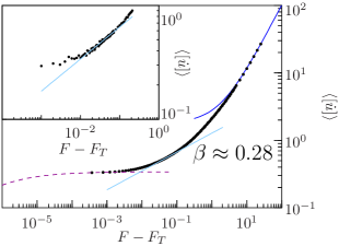
Figure 8: Velocity force relation for a sample with of longitudinal size $L=2048$ and transverse size $M=8192$. The time average was computed over $10^{10}$ time steps $\Delta t=2\cdot 10^{-2}$. We interpret the smaller slope at very low force differences as the beginning of the “single particle”-behavior $v^{-1}\propto\text{const}+(F-F_{T})^{-1/2}$ that has been derived in Ref. Duemmer and Krauth (2005), whereas at higher force difference the moving line with $v\sim F$ becomes apparent. The best value of $\beta$ depends on the threshold force used (here and in the inset we used $F_{T}\approx 1.79$), but we found consistent values of $\beta\approx 0.28$ for various sizes and samples. Inset: velocity force relation for one larger sample with $L=8192$ and $M=16384$. The time average was computed over $2^{20}$ time steps $\Delta t=2^{-6}$. There is a larger window with visible scaling.

We also tried to determine the velocity exponent $\beta$ directly. In the treatment of DLs, there is a significant discrepancy in the reported values of $\beta$, with either $\beta\approx 0.33$ Duemmer and Krauth (2005) or $\beta\approx 0.25$ Ferrero et al. (2013a). These were determined by means of two slightly different approaches: one can either determine (as in Duemmer and Krauth (2005)) the threshold force $F_{T,\text{sample}}$ for each sample and average $\overline{\langle[\dot{u}]\rangle(F-F_{T,\text{sample}})}$ or use $\langle v\rangle(F-\overline{F_{T,\text{sample}}})$ (as in Ferrero et al. (2013a)). We chose the first approach because $\overline{F_{T,\text{sample}}}$ cannot be clearly extracted from short-time dynamics scaling and, thus, the sample specific threshold force has to be determined anyway.

In Fig. 8 we show data for two single samples of sizes $L=2048$ and $L=8192$. We infer from our data

$$\beta\approx 0.28\text{.}$$ (51)

This agrees with the value $\beta\approx 0.29$ found in Ref. Lee and Kim (2006).

IV.4 Large forces

We have successfully confirmed the perturbative results of Sec. III.3, cp. Fig. 9, for large driving forces. Additionally, we checked that the roughness exponent $\zeta$ of the SDL takes its thermal value $\zeta_{th}=3/2$ for sufficiently large driving forces.

An interesting (and maybe counterintuitive) result is that increasing the force leads to a decrease in the “effective” temperature. We show this in Fig. 10 using the time averaged width (cp. eq. (8)) of the line as function of the force. We expect the width $w$ to scale as $w^{2}\sim L_{p}^{2}(L/L_{p})^{2\zeta}$ with an effective persistence length $L_{p}$ of the SDL. For purely thermal fluctuations we have $\zeta=\zeta_{th}=3/2$ and $L_{p}\sim 1/T$ Kleinert (2006); Kierfeld et al. (2006b). For the static SDL in disorder, on the other hand, we found a disorder-induced persistence length which is independent of temperature in the low-temperature phase of the SDL and which is minimal at the delocalization threshold Boltz and Kierfeld (2012, 2013). For the dynamic depinning, on the other hand, the simulation results in Fig. 10 show an increase of the SDL width at depinning, followed by a decrease $w\sim F^{-1}$ at high forces, where the roughness exponent assumes its thermal value $\zeta=\zeta_{th}=3/2$ again. This is consistent with a behavior $w^{2}\sim L^{3}/L_{p}$ with $L_{p}\sim F$ and, thus, an “effective” temperature $T_{\rm eff}\sim F^{-1}$ that decreases with driving force $F$. This can be rationalized from the FRG approach by noting that for high velocities the disorder contributes in form of an additional thermal noise corresponding to a temperature $T_{\text{eff}}\sim v\int\Delta$ Chauve et al. (2000). At high forces the line is far from the threshold and, thus, $\int\Delta$ should be close to the RB-disorder value of $\int\Delta=0$. The observed behavior $T_{\rm eff}\sim F^{-1}$ implies $\int\Delta\sim F^{-2}$ because $v\sim F$.

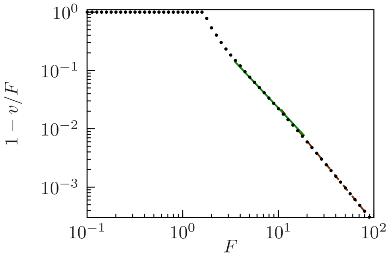
Figure 9: The deviation from the asymptotic $v\sim F$ for large forces in one sample. The green solid line is the perturbative result as given by eq. (38), the brown dashed line is given by $1-v/F\sim F^{-2}$. A similar cross-over to the single-particle behavior has been observed for the DL Dong et al. (1993). We used an Euler integration scheme with $2^{20}$ small time steps $\Delta t=2^{-10}$ to accurately simulate the system even for large forces. For steady state results the time average was performed only over the last $2^{19}$ time steps. The system has lateral size $L=64$ and transverse size $M=512$.

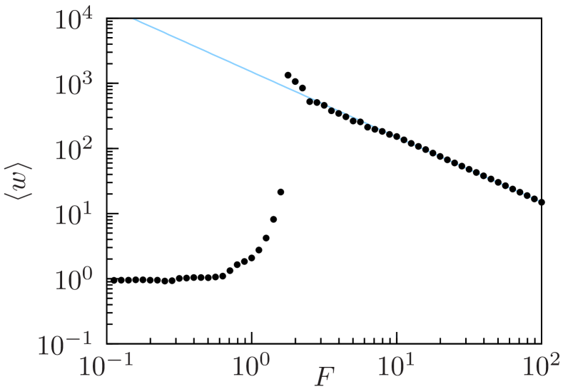
Figure 10: Time averaged width for a sample with $L=M=512$. The time average was performed over $2^{30}$ time steps. The line is maximally rough at the threshold, which is consistent with a “shockwave” motion, where small segments of the line move whilst the rest is blocked. At higher forces the width reduces with the force, which could be interpreted as a decrease of the effective temperature or, analogously, an increase in the effective persistence length. The solid line is a guide to the eye showing the $F^{-1}$ trend of the width.

IV.5 Confinement in a moving parabolic potential

A different approach Le Doussal (2006); Le Doussal and Wiese (2007); Middleton et al. (2007); Rosso et al. (2007) to compute the threshold force and, additionally, the effective disorder correlation functions is to pull the line very slowly with a spring. This means to introduce a parabolic potential acting on each line segment according to

$$V_{\text{par}}(u,t) =m^{2}(u-w(t))^{2}$$ (52)

and move the center $w(t)$ of the parabolic potential moves with a (small) constant velocity $\dot{w}=\text{const}>0$. We call $m^{2}$ the strength of the potential. The underlying idea is essentially that the force $F(\dot{w})$ exerted by the parabolic potential on the line as it moves forward becomes the threshold force for $m\rightarrow 0$, $\dot{w}\rightarrow 0$. More precisely, it was found for the DL that

$$\langle w-[u(w)]\rangle m^{2}=F_{T}+Cm^{2-\zeta}$$

with some constant $C$ (from now on, we assume that $\dot{w}$ is sufficiently small). For general $a$, the expected corrections due to finite values of $m$ have to be adjusted to account for the different elasticity. The length scale $L_{m}$ at which the confinement through the parabolic potential becomes relevant follows from balancing the elastic and the potential energy per length

$$u^{2}/L^{2a}\sim m^{2}u^{2}$$

$$L_{m}^{a}\sim m^{-1}$$

$L_{m}$ is the length of independently adjusting line-segments. Averaging over all $w$, i.e., averaging over disorder, typical displacements scale as $u_{m}\sim L_{m}^{\zeta}$. This leads to effective forces scaling as

$$F_{m} \sim m^{2}u_{m}\sim m^{2}L_{m}^{\zeta}$$ (53)

$$\sim m^{2-\zeta/a},$$ (54)

which includes the aforementioned DL result ($a=1$). A different approach Ferrero et al. (2013a) leading to the same result would be to use the known scaling of the finite-size corrections to the threshold force in one sample $F_{T}(L)-F_{T}\sim L^{-1/\nu}$ together with the notion that the relevant length scale is imposed by the parabolic potential and therefore given by $L_{m}\sim m^{-1/a}$. The confinement splits the line into independent segments of length $L_{m}$ and, therefore, one gets $F_{m}=F_{T}(L_{M})-F_{m}m^{1/\nu a}$. Using eq. (18) one finds $1/(\nu a)=2-\zeta/a$ and, thus, these two approaches are equivalent. In this derivation it is also clear that there will be deviations for very small $a$ when $L_{m}$ exceeds $L$.

As the line is constantly moved forward we chose to change the implementation of the potential. We still have a fixed amount $M$ of potential values (knots for the cubic spline), but we update the potential “on-the-fly” as the line is moved forward. Every time a segment of the line reaches a new quarter of $M$, we update the quarter that has the greatest distance to the current location and compute the splines [in principle, this changes the spline at the current location of the line, but the change is negligibly small if $M$ is large enough (we used $M=1024$)]. Our motivation for this scheme was to avoid finite-size-effects in the transverse direction and to be able to compute the disorder average as a time average. In Fig. 11 we show that our data are consistent with $\zeta\approx 2.0$.

Furthermore, this setup allows for a direct measurement of the effective force correlation function and hence a validation of the renormalization group solution. This is achieved via the second cumulant of $u(t)-w(t)$ as

$$\langle(u(t)-w(t))(u(t^{\prime})-w^{\prime}(t^{\prime}))\rangle_{c}m^{4}\propto\Delta(w-w^{\prime})\text{.}$$ (55)

This contribution is closely related to the shape of the force correlation function Le Doussal et al. (2002), see eq. (33). The existence of a non-vanishing $\Delta^{\prime}(0^{+})$, often referred to as “cusp”, is a sign of the non-analyticity of the correlation function. We show our results in Fig. 12, which demonstrate promising agreement with the functional renormalization group fixed point function.

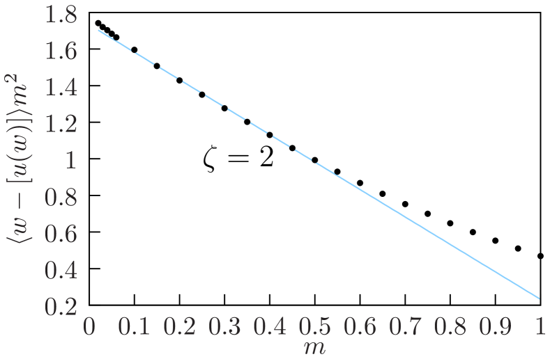
Figure 11: Time average of the net force that the parabolic potential exerts on the center of motion of the line ($L=256$, $M=1024$). The solid line is a fit for $m\in[0.1,0.5]$ with $\zeta=2$ yielding $F_{T}=1.733\pm 0.007$. The velocity of the parabolic potential was $\dot{w}=10^{-6}$. The shape of the numerical results and their deviations from the analytical expectation resemble the findings for the DL in Ref. Middleton et al. (2007). The value $F_{T}=1.733$ deviates from the value found above because of the differing system size.

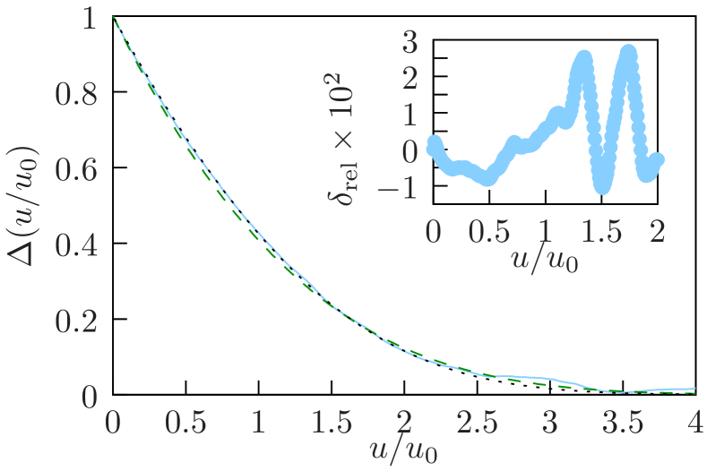
Figure 12: Numerical determination of the disorder correlator $\Delta(u)$ according to (55) with $m^{2}=10^{-2}$. The data are taken from the same simulation as for Fig. 11. The dashed (green) line is the one-loop solution and the dotted (black) line is the two-loop solution, see Sec. III.2 and Ref. Le Doussal et al. (2002). The length scale $u_{0}$ is determined via $\int\mathrm{d}u\Delta{(u/u_{0})}=1$. The inset shows the relative difference between the two-loop solution $\Delta_{2L}$ and the numerically determined values $\Delta$, i.e., $\delta_{\text{rel}}=(\Delta-\Delta_{2L})/\Delta_{2L}$ for small $u/u_{0}$.

IV.6 Finite temperatures – thermal rounding

The finite mean velocity at arbitrarily small non-zero temperatures is only visible for very long simulation times, Thus, the regime in which creep/TAFF behavior should occur is not accessible for us.

The thermal rounding exponent $\psi$, as defined in eq. (45), can be interpreted in a slightly different way, that we feel is more apt for the interpretation of numerical data. Moving away from the threshold at $F=F_{T}$ and $T=0$ the velocity scales as $(F-F_{T})^{\beta}$ or $T^{\psi}$, respectively. Thus, a finite temperature at $F_{T}$ can effectively be seen as a contribution to the pulling force with

$$F-F_{T}\sim T^{\eta}$$ (56)

and $\eta=\psi/\beta$. Adapting our previous statements the perturbative conjecture would be $\eta=1/(1+2\beta)$. In Fig. 13 we show that using this rescaling we can collapse data for the velocity as a function of $F-F_{T}$ at $T=0$ and for the velocity at the threshold $F=F_{T}$ as a function fo temperature. The data collapse is consistent with $\eta=1/(1+2\beta)$ and $\beta\approx 0.28$.

We compare our numerical results for the thermal rounding of the depinning transition for the DL and the SDL in Fig. 14. Surprisingly, we find no evidence for a qualitative change at a finite temperature that could be associated with the localization transition in the static problem. This could either mean that the change is too subtle to be apparent within our numerics or that, in terms of the FRG, a finite velocity $v>0$ implies that the relevant fixed point is one featuring $v>0$ and $T=0$, which would make the transition at finite temperature irrelevant for a moving line.

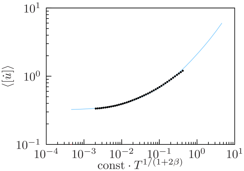
Figure 13: Time average of the velocity at the threshold force for finite temperatures. We used $\beta=0.28$ or $\eta=0.64$ in the rescaling of the temperature (black points). The data collapse with data for the velocity as a function of $F-F_{T}$ at $T=0$ (blue line) after rescaling using eq. (56). The data for the velocity as a function of $F-F_{T}$ at $T=0$ and, thus, all system parameters but the temperature are the same as for Fig. 8.

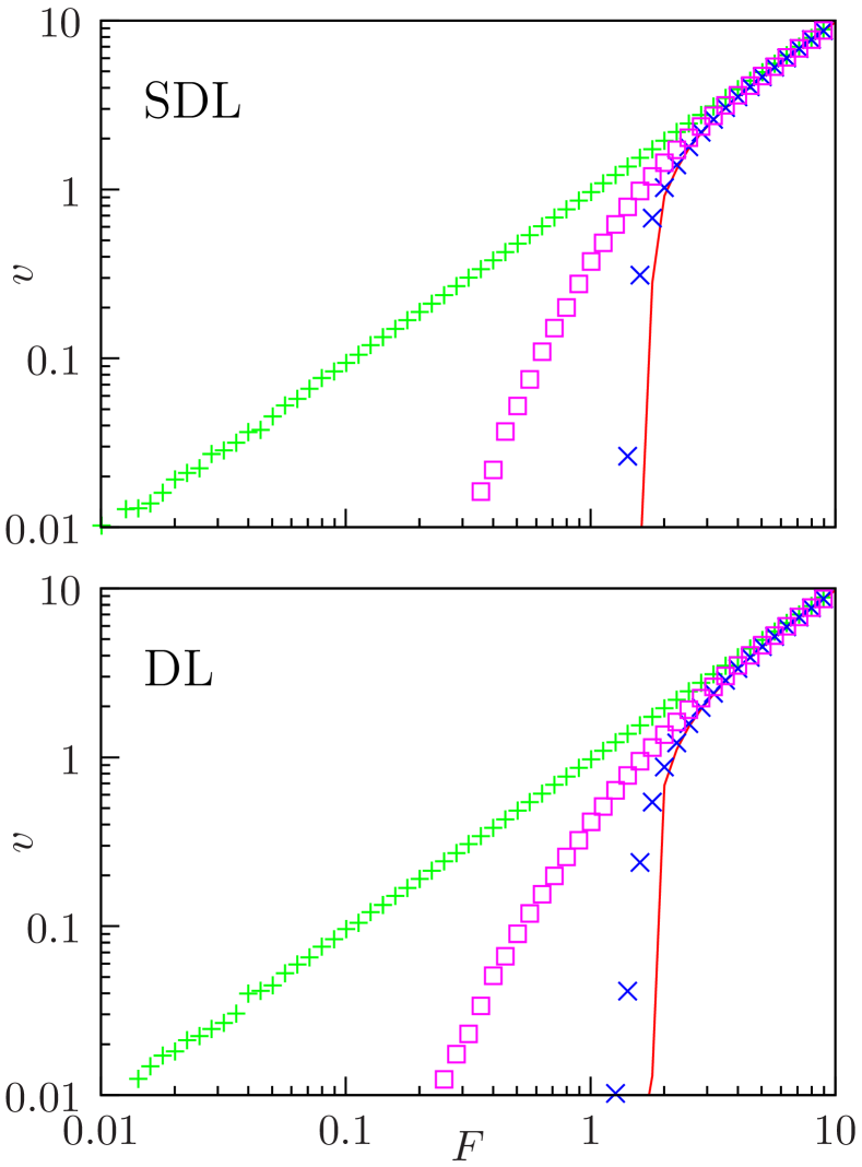
Figure 14: Velocity of the line as a function of the driving force at four different temperatures (solid line: $T=0$). For a better comparison we show data for a SDL and a DL in the same disorder. Note that as the same disorder was used the velocities are very similar, but not identical. All system parameters but the temperature are the same as for Fig. 8.

V Direct computation of threshold force – Middleton’s theorems

In the study of the depinning of directed lines two important properties have been found Middleton (1992): a) the “no-passing” theorem, which states that two lines in the same disorder realization that do not cross each other at a given time will never cross each other; b) if each segment of the line has at some point in time a non-negative velocity the velocity will remain non-negative for all times; this has been referred to as “no-return” property Kolton et al. (2006b). The no-passing theorem is believed to hold for every convex next-neighbor elastic energy. The combination of these properties allows for a fast and precise algorithm to determine the threshold force directly Rosso and Krauth (2002).

With regard to the no-passing theorem we consider the following situation: two lines $z_{1}$, $z_{2}$ in the same medium that touch each other at exactly one point, that is there is one $x$ with $z_{1}(x)=z_{2}(x)$ and $z_{1}(x^{\prime})>z_{2}(x^{\prime})$ for $x\neq x^{\prime}$. For the DL, it follows that $v_{1}(x)>v_{2}(x)$. As both lines touch each other in $x$ a possibly differing velocity of the two lines is due to the elastic forces. In the discrete version we then have $v_{1}(x)>v_{2}(x)$, because $(z_{1}(x-1)-z_{2}(x-1))+(z_{1}(x+1)-z_{2}(x+1))>0$. This does not work for the SDL, because the difference in velocity

$$v_{1}(x)-v_{2}(x)=- (z_{1}(x-2)-z_{2}(x-2))$$

$$- (z_{1}(x+2)-z_{2}(x+2))$$

$$+4 (z_{1}(x-1)-z_{2}(x-1))$$

$$+4 (z_{1}(x+1)-z_{2}(x+1))$$ (57)

can take any value. We visualize this in Fig. 15.

Therefore, the SDL does not necessarily explore “new” regions of the disorder potential. A line that moves back and forth “knows” essentially the whole potential at any point. This could be an explanation for the two distinct correlation length exponents $\nu$ and $\nu_{\text{FS}}$ that we found for the SDL, see eq. (50). The fact that Middleton’s theorems guarantee that $u(x)$ is a monotonic function of time is also used in the evaluation of ambiguous vertices within the FRG treatment in Ref. Le Doussal et al. (2002). However, we feel that coming from a moving line with $v>0$ the quasistatic depinning limit is still well defined for the SDL, because the long time limit of the roughness is (for finite $L$) finite and, therefore, all segments will eventually move on average with the same velocity. The agreement of the FRG with our numerical results supports that there is no fundamental problem with the applicability of the FRG for the SDL. Still, there is definitely room and need for a more rigorous analysis.

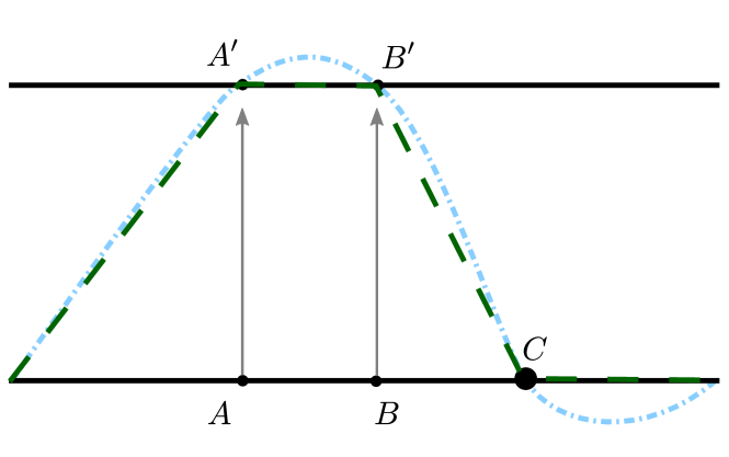
Figure 15: Cartoon exemplifying the difference in the evolution of a DL and a SDL starting from the lower horizontal conformation. Let the potential be such, that the line points at $A$ and $B$ are forced to move to $A^{\prime}$ and $B^{\prime}$, whereas the ends and the line point at $C$ cannot move. The DL (green dashed line) does not pass the blocked upper line and also does not cross the lower line. The SDL (blue dash-dotted line) seeks to reduce the curvature and, consequently, does cross both lines.

VI Conclusion

We studied the depinning of SDLs from disorder (RF or RB) in $1+1$ dimensions due to a driving force. Using scaling arguments, analytical FRG calculations, and extensive numerical simulations, we characterized the critical behavior at and around the depinning transition. Our study revealed some characteristic differences in depinning behavior between SDLs and DLs governed by tension.

The resulting equation of motion for the SDL in disorder is equivalent to the Herring-Mullins equation for surface growth, which is governed by surface diffusion rather than surface tension, in quenched disorder. Our results also apply to semiflexible polymers with contour lengths smaller than their persistence length, which are pulled over a disordered surfaces or driven through a random medium.

We show that Middleton’s theorems do not apply to SDLs. Nevertheless we find a well-defined threshold force $F_{T}$ for depinning. Likewise, critical exponents characterizing roughness and the dynamics of depinning can be defined and numerically determined for the SDL as for the DL. The SDL represents an own dynamical universality class with a different set of exponents. Our extensive numerical data is best described by the set (50) of critical exponents which is also consistent with scaling relations, see section III.1. We also investigated the behavior of the SDL persistence length, which exhibits a characteristic non-monotonous force-dependence through the depinning transition (see Fig. 10).

We transferred functional renormalization group results to the elasticity of stiff interfaces, which allows us to derive analytical results or bounds for critical exponents (see section III.2). We find satisfying agreement of these analytical predictions with our numerical work. Our results indirectly imply that the depinning threshold is associated with two distinct correlation length exponents $\nu$ and $\nu_{\text{FS}}$. To our knowledge this would be the first occurrence of such behavior in a non-periodic system. This result could be linked to the non-validity of Middleton’s no-passing theorem.

Our findings for the critical exponents at the threshold force disagree in parts with previous numerical work, which suggests that further work, especially on much larger systems, might be helpful to settle these exponents.

For finite temperatures, the depinning of a SDL is an interesting problem because, at equilibrium (no pulling force), the problem features a disorder-driven localization transition at a finite temperature. Such a transition is absent for the DL, which remains in a localized disorder-dominated phase for all temperatures. Surprisingly, the numerical results for a comparison of the thermal rounding of the force-driven depinning transition do not show any qualitative difference between DLs and SDLs, see Fig. 14. In a renormalization group sense, this might imply that the force-driven depinning and the temperature-driven delocalization are not described by the same fixed point.

VII Acknowledgments.

We acknowledge financial support by the Deutsche Forschungsgemeinschaft (KI 662/2-1).

Appendix A Bounds for the dynamical exponent $z$

In Ref. Le Doussal et al. (2002) the dynamical exponent $z$ has been found to be to two-loop order

$$z =4-2/9\varepsilon+\varepsilon^{2}\left(\frac{\zeta_{2}}{3}-\frac{2X^{(2a)}}{27}+\frac{Y^{(2a)}}{54}\right)$$ (58)

with $\zeta_{2}$, $X^{(2a)}$ the same as in the main text and

$$Y^{(2a)} =X^{(2a)}+\varepsilon\left(\frac{2I_{\eta}}{(\varepsilon I_{1})^{2}}-\frac{1}{\varepsilon}\right)\text{,}$$ (59)

where we use $I_{\eta}$ as shorthand notation for the aforementioned correction to friction for the SDL

$$I_{\eta}=I_{\eta}^{(4)} =\int_{q_{1},q_{2}}\frac{1}{\left(q_{1}^{2}+m^{2}\right)^{2}\left(q_{2}^{2}+m^{2}\right)^{4}}\times$$ (60)

$$\frac{1}{\left(\left(q_{2}^{2}+m^{2}\right)^{2}+\left(\left(q_{1}-q_{2}\right)^{2}+m^{2}\right)^{2}\right)}$$ (61)

and $I_{1}$ is the one-loop integral given by

$$I_{1} =m^{-\varepsilon}\frac{\Gamma(\varepsilon/2)}{\Gamma(4)}\left(\int_{q}\mathrm{e}^{-q^{2}}\right)\text{.}$$ (62)

Using $I_{\eta}\geq 0$ we find the lower bound

$$z\geq 1.8607\text{.}$$ (63)

For an upper bound we note that in any dimension (any value of $\epsilon$) the following inequality holds

$$I_{\eta}\leq J_{\eta} =\int_{q_{1},q_{2}}\frac{1}{(q_{1}^{2}+m^{2})^{2}(q_{2}^{2}+m^{2})^{4}(q_{3}^{2}+m^{2})^{2}}$$

and $J_{\eta}$ can be evaluated to leading order in $\epsilon$ via Laplace transforms

$$J_{\eta} =\frac{1}{\Gamma(4)}\int\limits_{\begin{subarray}{c}s_{1},s_{2},s_{3}>0\\ q_{1},q_{2}\end{subarray}}s_{1}s_{2}^{3}s_{3}\times$$

$$~{}~{}\times\mathrm{e}^{-s_{1}(q_{1}^{2}+m^{2})-s_{2}(q_{2}^{2}+m^{2})-s_{3}(q_{3}^{2}+m^{2})}$$

$$=\frac{\left(\int_{q}\mathrm{e}^{-q^{2}}\right)^{2}}{\Gamma(4)}\int\limits_{s_{1},s_{2},s_{3}>0}\frac{s_{1}s_{2}^{3}s_{3}\mathrm{e}^{-m^{2}(s_{1}+s_{2}+s_{3})}}{(s_{1}s_{2}+s_{2}s_{3}+s_{2}s_{3})^{d/2}}$$

Substituting $s_{2}\rightarrow s_{1}s_{2}$, $s_{3}\rightarrow s_{1}s_{3}$ gives

$$J_{\eta} =\frac{\left(\int_{q}\mathrm{e}^{-q^{2}}\right)^{2}}{\Gamma(4)}\int\limits_{s_{1},s_{2},s_{3}>0}\frac{s_{1}^{7-d}s_{2}^{3}s_{3}\mathrm{e}^{-m^{2}s_{1}(1+s_{2}+s_{3})}}{(s_{2}+s_{3}+s_{2}s_{3})^{d/2}}$$

$$=\frac{\left(\int_{q}\mathrm{e}^{-q^{2}}\right)^{2}}{\Gamma(4)}\Gamma(\varepsilon)m^{-2\varepsilon}\times$$

$$~{}~{}\times\int\limits_{s_{2},s_{3}>0}\frac{s_{2}^{3}s_{3}}{(s_{2}+s_{3}+s_{2}s_{3})^{d/2}}\frac{1}{(1+s_{2}+s_{3})^{\varepsilon}}$$

$$=\frac{\left(\int_{q}\mathrm{e}^{-q^{2}}\right)^{2}}{\Gamma(4)}\Gamma(\varepsilon)m^{-2\varepsilon}J$$

$$J =\int\limits_{s_{2},s_{3}>0}\frac{s_{2}^{3}s_{3}}{(s_{2}+s_{3}+s_{2}s_{3})^{4}}\frac{(s_{2}+s_{3}+s_{2}s_{3})^{\varepsilon/2}}{(1+s_{2}+s_{3})^{\varepsilon}}$$

$$=\int\limits_{s_{2},s_{3}>0}\frac{s_{2}s_{3}}{(1+s_{3}+s_{2}s_{3})^{4}}\frac{s_{2}^{\varepsilon/2}(1+s_{3}+s_{2}s_{3})^{\varepsilon/2}}{(1+s_{2}+s_{2}s_{3})^{\varepsilon}}$$

$$=J_{1}+J_{2}+J_{3}$$

In the second to last step we substituted $s_{3}\rightarrow s_{2}s_{3}$. We have divided the integration in three terms to isolate the (important) divergent part.

$$J_{1} =\int_{1}^{\infty}\mathrm{d}s_{2}\int_{0}^{\infty}\mathrm{d}s_{3}\frac{s_{2}s_{3}}{(1+s_{3}+s_{2}s_{3})^{4}}\times$$

$$~{}~{}\times\frac{s_{2}^{\varepsilon/2}(1+s_{3}+s_{2}s_{3})^{\varepsilon/2}}{(1+s_{2}+s_{2}s_{3})^{\varepsilon}}$$

$$=-\frac{1}{12}+\frac{\ln{2}}{6}+\mathcal{O}(\varepsilon)$$ (64)

$$J_{2} =\int_{0}^{\infty}\mathrm{d}s_{3}\int_{0}^{1}\mathrm{d}s_{2}\left[\frac{s_{2}s_{3}}{(1+s_{3}+s_{2}s_{3})^{4}}\times\right.$$

$$\left.~{}~{}\times\frac{s_{2}^{\varepsilon/2}(1+s_{3}+s_{2}s_{3})^{\varepsilon/2}}{(1+s_{2}+s_{2}s_{3})^{\varepsilon}}-\frac{s_{2}^{1+\varepsilon/2}s_{3}}{(1+s_{2}s_{3})^{4+\varepsilon/2}}\right]$$

$$=-\frac{1}{12}-\frac{\ln{4}}{6}+\mathcal{O}(\varepsilon)$$ (65)

$$J_{3} =\int_{0}^{\infty}\mathrm{d}s_{3}\int_{0}^{1}\mathrm{d}s_{2}\frac{s_{2}^{1+\varepsilon/2}s_{3}}{(1+s_{2}s_{3})^{4+\varepsilon/2}}$$

$$=\frac{1}{3\varepsilon}-\frac{5}{18}$$ (66)

Thus collecting all terms we find

$$J_{\eta} =\frac{\left(\int_{q}\mathrm{e}^{-q^{2}}\right)^{2}}{\Gamma(4)}\Gamma(\varepsilon)m^{-2\varepsilon}(J_{1}+J_{2}+J_{3})$$

$$=\frac{6}{4}(J_{1}+J_{2}+J_{3})(\varepsilon I_{1})^{2}$$ (67)

and

$$Y^{(4)} \leq X^{(4)}+\varepsilon\left(\frac{2J_{\eta}}{(\varepsilon I_{1})^{2}}-\frac{1}{\varepsilon}\right)$$

$$\leq-\frac{2}{3}+\mathcal{O}(\varepsilon)\text{,}$$ (68)

which ultimately yields

$$z \leq 2.3144,$$ (69)

i.e., eq. (31) in the main text.

References

- Halpin-Healy and Zhang (1995) T. Halpin-Healy and Y.-C. Zhang, Phys. Rep. 254 (1995).
- Blatter et al. (1994) G. Blatter, M. V. Feigelman, V. B. Geshkenbein, A. I. Larkin, and V. M. Vinokur, Rev. Mod. Phys. 66, 1125 (1994).
- Paczuski et al. (1996) M. Paczuski, S. Maslov, and P. Bak, Phys. Rev. E 53, 414 (1996).
- Feigel’man (1983) M. Feigel’man, Sov. Phys. JETP 58, 1076 (1983).
- Sneddon et al. (1982) L. Sneddon, M. C. Cross, and D. S. Fisher, Phys. Rev. Lett. 49, 292 (1982).
- Middleton (1992) A. A. Middleton, Phys. Rev. Lett. 68, 670 (1992).
- Chauve et al. (2000) P. Chauve, T. Giamarchi, and P. Le Doussal, Phys. Rev. B 62, 6241 (2000).
- Le Doussal et al. (2002) P. Le Doussal, K. J. Wiese, and P. Chauve, Phys. Rev. B 66, 174201 (2002).
- Duemmer and Krauth (2005) O. Duemmer and W. Krauth, Phys. Rev. E 71, 061601 (2005).
- Le Doussal and Wiese (2007) P. Le Doussal and K. J. Wiese, EPL 77, 66001 (2007).
- Middleton et al. (2007) A. A. Middleton, P. Le Doussal, and K. J. Wiese, Phys. Rev. Lett. 98, 155701 (2007).
- Rosso et al. (2007) A. Rosso, P. Le Doussal, and K. J. Wiese, Phys. Rev. B 75, 220201 (2007).
- Ferrero et al. (2013a) E. E. Ferrero, S. Bustingorry, and A. B. Kolton, Phys. Rev. E 87, 032122 (2013a), a detailed description of the numerical implementation can be found in the supplemental material at http://link.aps.org/supplemental/10.1103/PhysRevE.87.032122. See also Ferrero et al. (2013b).
- Narayan and Fisher (1992a) O. Narayan and D. S. Fisher, Phys. Rev. B 46, 11520 (1992a).
- Narayan and Fisher (1992b) O. Narayan and D. S. Fisher, Phys. Rev. Lett. 68, 3615 (1992b).
- Nattermann et al. (1992) T. Nattermann, S. Stepanow, L.-H. Tang, and H. Leschhorn, J. Phys. II France 2, 1483 (1992).
- Herring (1951) C. Herring, in The Physics of Powder Metallurgy, edited by W. E. Kingston (McGraw-Hill, New York, 1951) p. 143.
- Mullins (1957) W. W. Mullins, J. Appl. Phys. 28, 333 (1957).
- Park and Kim (2000) K. Park and I.-M. Kim, Phys. Rev. E 61, 4606 (2000).
- Lee and Kim (2006) C. Lee and J. M. Kim, Phys. Rev. E 73, 016140 (2006).
- Liu et al. (2008) H. Liu, W. Zhou, Q.-M. Nie, and Q.-H. Chen, Phys. Lett. A 372, 7077 (2008).
- Song and Kim (2006) H. S. Song and J. M. Kim, J. Korean Phys. Soc. 49, 1520 (2006).
- Kierfeld et al. (2006a) J. Kierfeld, P. Gutjahr, T. Kühne, P. Kraikivski, and R. Lipowsky, J. Comput. Theor. Nanosci. 3, 898 (2006a).
- Bundschuh and Lässig (2002) R. Bundschuh and M. Lässig, Phys. Rev. E 65, 061502 (2002).
- Boltz and Kierfeld (2012) H.-H. Boltz and J. Kierfeld, Phys. Rev. E 86, 060102(R) (2012).
- Boltz and Kierfeld (2013) H.-H. Boltz and J. Kierfeld, Phys. Rev. E 88, 012103 (2013).
- Bundschuh et al. (2000) R. Bundschuh, M. Lässig, and R. Lipowsky, Eur. Phys. J. E 3, 295 (2000).
- Kierfeld and Lipowsky (2005) J. Kierfeld and R. Lipowsky, J. Phys. A: Math. Gen. 38, L155 (2005).
- Harris and Hearst (1966) R. Harris and J. Hearst, J. Chem. Phys. 44, 2595 (1966).
- Kratky and Porod (1949) O. Kratky and G. Porod, Recl. Trav. Chim. Pays-Bas 68, 1106 (1949).
- Barabási and Stanley (1995) A.-L. Barabási and H. E. Stanley, Fractal concepts in surface growth (Cambridge University Press, 1995).
- Das Sarma et al. (1994) S. Das Sarma, S. V. Ghaisas, and J. M. Kim, Phys. Rev. E 49, 122 (1994).
- Racz and Plischke (1994) Z. Racz and M. Plischke, Phys. Rev. E 50, 3530 (1994).
- Note (1) With a full set of parameters the equation would read , which reduces to the given form by rescaling , and with given by the discretization, and .
- Brú et al. (1998) A. Brú, J. M. Pastor, I. Fernaud, I. Brú, S. Melle, and C. Berenguer, Phys. Rev. Lett. 81, 4008 (1998).
- Edwards and Wilkinson (1982) S. F. Edwards and D. R. Wilkinson, Proc. Roy. Soc. London, Ser. A 381, 17 (1982).
- Kardar (1987) M. Kardar, Nucl. Phys. B 290, 582 (1987).
- Chauve et al. (2001) P. Chauve, P. Le Doussal, and K. J. Wiese, Phys. Rev. Lett. 86, 1785 (2001).
- Le Doussal et al. (2004) P. Le Doussal, K. J. Wiese, and P. Chauve, Phys. Rev. E 69, 026112 (2004).
- Belanger and Young (1991) D. Belanger and A. Young, J. Magn. Magn. Mater. 100, 272 (1991).
- Seppälä et al. (1998) E. T. Seppälä, V. Petäjä, and M. J. Alava, Phys. Rev. E 58, R5217 (1998).
- Lee et al. (2000) J. H. Lee, S. K. Kim, and J. M. Kim, Phys. Rev. E 62, 3299 (2000).
- Fisher (1986) D. S. Fisher, Phys. Rev. Lett. 56, 1964 (1986).
- Narayan and Fisher (1993) O. Narayan and D. S. Fisher, Phys. Rev. B 48, 7030 (1993).
- Bolech and Rosso (2004) C. J. Bolech and A. Rosso, Phys. Rev. Lett. 93, 125701 (2004).
- Middleton and Fisher (1991) A. A. Middleton and D. S. Fisher, Phys. Rev. Lett. 66, 92 (1991).
- Chayes et al. (1986) J. T. Chayes, L. Chayes, D. S. Fisher, and T. Spencer, Phys. Rev. Lett 57, 2999 (1986).
- Larkin (1970) A. I. Larkin, Sov. Phys. JETP 31 (1970).
- Leschhorn (1993) H. Leschhorn, Physica A 195, 324 (1993).
- Ioffe and Vinokur (1987) L. B. Ioffe and V. M. Vinokur, J. Phys. C 20, 6149 (1987).
- Nattermann et al. (1990) T. Nattermann, Y. Shapir, and I. Vilfan, Phys. Rev. B 42, 8577 (1990).
- Lemerle et al. (1998) S. Lemerle, J. Ferré, C. Chappert, V. Mathet, T. Giamarchi, and P. Le Doussal, Phys. Rev. Lett. 80, 849 (1998).
- Anderson and Kim (1964) P. W. Anderson and Y. B. Kim, Rev. Mod. Phys. 36, 39 (1964).
- Kes et al. (1989) P. Kes, J. Aarts, J. Van den Berg, C. Van der Beek, and J. Mydosh, Supercond. Sci. Tech. 1, 242 (1989).
- Kolton et al. (2009) A. B. Kolton, A. Rosso, T. Giamarchi, and W. Krauth, Phys. Rev. B 79, 184207 (2009).
- (56) L. H. Tang and S. Stepanow, Unpublished, as cited in Chauve et al. (2000).
- Bustingorry et al. (2008) S. Bustingorry, A. B. Kolton, and T. Giamarchi, EPL 81, 26005 (2008).
- Bustingorry et al. (2012) S. Bustingorry, A. B. Kolton, and T. Giamarchi, Phys. Rev. E 85, 021144 (2012).
- Note (2) Our simulations were performed on a Tesla C2070. We used the CUDA Toolkit, version 5.0.NVIDIA Corporation .
- Rosso and Krauth (2002) A. Rosso and W. Krauth, Phys. Rev. E 65, 025101 (2002).
- Kolton et al. (2006a) A. B. Kolton, A. Rosso, E. V. Albano, and T. Giamarchi, Phys. Rev. B 74, 140201 (2006a).
- Kleinert (2006) H. Kleinert, Path Integrals in Quantum Mechanics, Statistics, Polymer Physics, and Financial Markets (World Scientific, Singapore, 2006).
- Kierfeld et al. (2006b) J. Kierfeld, R. Lipowsky, and P. Gutjahr, Europhys. Lett. , 994 (2006b).
- Dong et al. (1993) M. Dong, M. C. Marchetti, A. A. Middleton, and V. Vinokur, Phys. Rev. Lett. 70, 662 (1993).
- Le Doussal (2006) P. Le Doussal, EPL 76, 457 (2006).
- Kolton et al. (2006b) A. B. Kolton, A. Rosso, T. Giamarchi, and W. Krauth, Phys. Rev. Lett. 97, 057001 (2006b).
- Ferrero et al. (2013b) E. E. Ferrero, S. Bustingorry, and A. B. Kolton, Phys. Rev. E 87, 069901(E) (2013b).
- (68) NVIDIA Corporation, “CUDA C Programming Guide,” Available online: http://docs.nvidia.com/cuda/cuda-c-programming-guide/.