Numerical simulations of X-rays Free Electron Lasers (XFEL)

Abstract.

We study a nonlinear Schrödinger equation which arises as an effective single particle model in X-ray Free Electron Lasers (XFEL). This equation appears as a first-principles model for the beam-matter interactions that would take place in an XFEL molecular imaging experiment in [7]. Since XFEL is more powerful by several orders of magnitude than more conventional lasers, the systematic investigation of many of the standard assumptions and approximations has attracted increased attention.

In this model the electrons move under a rapidly oscillating electromagnetic field, and the convergence of the problem to an effective time-averaged one is examined. We use an operator splitting pseudo-spectral method to investigate numerically the behaviour of the model versus its time-averaged version in complex situations, namely the energy subcritical/mass supercritical case, and in the presence of a periodic lattice.

We find the time averaged model to be an effective approximation, even close to blowup, for fast enough oscillations of the external field. This work extends previous analytical results for simpler cases [1].

1. Introduction

In this paper we study a first principles model for beam-matter interaction in X-ray free electron lasers (XFEL) [6, 7]. Recent developments using XFEL include the observation of the motion of atoms [3], measuring the dynamics of atomic vibrations [8], biomolecular imaging [15] etc. The fundamental model for XFEL is the following nonlinear Schrödinger equation

(1.1) $$\left\{\begin{aligned} &i\hbar{\partial}_{t}\psi=\frac{1}{2m}(i\hbar\nabla-e\boldsymbol{\rm{A}})^{2}\psi+Ze\frac{1}{|\boldsymbol{\rm{x}}|}\psi+e^{2}(|\cdot|^{-1}\ast|\psi|^{2})\psi-\lambda|\psi|^{\sigma}\psi,\\ &\psi(t,\boldsymbol{\rm{x}})|_{t=0}=\psi_{0}(\boldsymbol{\rm{x}}),\end{aligned}\right.$$

on $\mathbb{R}^{3}$. Here $m_{e}$ is the electron mass, $e$ the electron charge, $Z$ the atomic number and $\hbar$ is the scaled (by $2\pi$) Planck constant. The constant $\lambda>0$ measures the strenght of the local attractive nonlinearity with power $\sigma>0$, in particular $\sigma=\frac{2}{3}$ and $\lambda=3e^{2}\left(\frac{3}{8\pi}\right)^{1/3}$ for the local Hartree-Fock approximation.

A solution $\psi=\psi(t,\boldsymbol{\rm{x}})$ of this Schrödinger equation can be considered as the wave function of an electron beam, interacting self-consistently through the repulsive Coulomb (Hartree) force, the attractive local Fock-type approximation with strength $\lambda$ and exponent $\sigma$ and interacting repulsively with an atomic nucleus, located at the origin. The vector field ${\boldsymbol{\rm{A}}}={\boldsymbol{\rm{A}}}(t)$ represents an external electromagnetic field, which we shall assume to depend on time $t$ only (not on position $\boldsymbol{\rm{x}}$).

In the experimental setup of interest [6, 7] the magnetic field is rapidly oscillating. This effect of oscillating external magnetic field appears often in the modelling of undulators; here the aim is to justify systematically the use of an effective, time-averaged magnetic field, in the presence of beam-matter interaction.

In [1] it was shown that, under appropriate assumptions, the solution of (1.1) can be approximated, in the asymptotic regime $|\omega|\gg 1$, by the solution of an effective, time-averaged Schrödinger initial value problem. The present work is a continuation of that line of investigation in more general contexts. More specifically, with the help of numerical simulations, we are able to tackle more detailed questions with respect to the role of the fast magnetic field, the mode of convergence, and attack problems with blowup. Moreover, we investigate the effect of a periodic lattice on the model.

1.1. The model

We scale the equation (1.1) by choosing a characteristic time scale $t_{c}$ and a characteristic spatial scale $x_{c}$. Defining the semiclassical parameter $\varepsilon=\frac{\hbar t_{c}}{2m_{e}x_{c}^{2}}$ we obtain after rescaling

$$i\varepsilon{\partial}_{t}\psi=(i\varepsilon\nabla-\boldsymbol{\rm{A}})^{2}\psi+\frac{c}{|x|}\psi+C_{1}(|\cdot|^{-1}\ast|\psi|^{2})\psi-a|\psi|^{\sigma}\psi$$

where $c=eZ\frac{t_{c}^{2}}{2m_{e}x_{c}}$, $C_{1}=e^{2}\frac{t_{c}^{6}}{8m_{e}^{3}x_{c}^{4}}$, $a=\lambda\left(\frac{t_{c}^{2}}{2m_{e}x_{c}^{2}}\right)^{\sigma+1}$. Here also $\psi$ and $\boldsymbol{\rm{A}}$ were scaled appropriately.

A standard transform is used to simplify the original equation, and bring it to a form more amenable to analysis as well as computation. By setting

(1.2) $$u(t,\boldsymbol{\rm{x}})=\psi\left(t,\boldsymbol{\rm{x}}+b(t)\right)\exp\left(\frac{i}{\varepsilon}\displaystyle\int_{0}^{t}{|\boldsymbol{\rm{A}}(s)|^{2}ds}\right),$$

where $b(t)=2\int_{0}^{t}\boldsymbol{\rm{A}}(s)ds$, one readily checks that $u$ satisfies the initial value problem

(1.3) $$\left\{\begin{aligned} &i\varepsilon\partial_{t}u=-\varepsilon^{2}\Delta u+\frac{c}{|\boldsymbol{\rm{x}}-b(t)|}u+C_{1}(|\cdot|^{-1}\ast|u|^{2})u-a|u|^{\sigma}u\\ &u^{\omega}(t,\boldsymbol{\rm{x}})\big{|}_{t=0}=u_{0}(\boldsymbol{\rm{x}}),\end{aligned}\right.$$

where $u_{0}:=\psi_{0}$. Now we choose the scales $x_{c},t_{c}$ such that $\varepsilon=1$ (thus relating $x_{c}$ and $t_{c}$ by $2m_{e}x_{c}^{2}=\hbar t_{c}$), since we are mostly interested in the fully quantum mechanical case, and we fix

$$b(t)=e(t)\sin(2\pi\omega t).$$

where $e:\mathbb{R}\to\mathbb{R}^{3}$ is a smooth vector field, slowly varying in time.We consider the large frequency case

$$|\omega|\gg\frac{{\rm sec}}{t_{c}}=\frac{\hbar}{2m_{e}}\left(\frac{{\rm meter}}{x_{c}}\right)^{2}\approx 5\times 10^{-3}\left(\frac{{\rm meter}}{x_{c}}\right)^{2}.$$

and study the asymptotic regime $|\omega|\to\infty$. In particular we shall investigate the convergence of solutions of

(1.4) $$\left\{\begin{aligned} &i\partial_{t}u^{\omega}=-\Delta u^{\omega}+V^{\omega}u^{\omega}+C_{1}(|\cdot|^{-1}\ast|u^{\omega}|^{2})u^{\omega}-a|u^{\omega}|^{\sigma}u^{\omega}\\ &u^{\omega}(t,\boldsymbol{\rm{x}})\big{|}_{t=0}=u_{0}(\boldsymbol{\rm{x}}),\end{aligned}\right.$$

where the fast oscillatory potential is given by

(1.5) $$V^{\omega}(t,x):=\frac{c}{|\boldsymbol{\rm{x}}-e(t)\sin(2\pi\omega t)|},$$

to solutions of the approximate problem (see [1] and Theorem 1 there)

(1.6) $$\left\{\begin{aligned} &i\partial_{t}u=-\Delta u+\langle V\rangle u+C_{1}(|\cdot|^{-1}\ast|u|^{2})u-a|u|^{\sigma}u\\ &u(t,\boldsymbol{\rm{x}})\big{|}_{t=0}=u_{0}(\boldsymbol{\rm{x}}),\end{aligned}\right.$$

with $\langle V\rangle$ is the time averaged potential given by

(1.7) $$\langle V\rangle(t,\boldsymbol{\rm{x}}):=\int_{0}^{1}\frac{c}{|\boldsymbol{\rm{x}}-e(t)\sin(2\pi s)|}ds.$$

We remark that (1.7) is well defined as the weak limit of $V^{\omega}$ defined in (1.5) in the space $L^{\infty}(\mathbb{R};L^{3-}(\mathbb{R}^{3})+L^{3+}(\mathbb{R}^{3}))$, as $|\omega|\to\infty$ (see [1] for more details). Passing back and forth between $u$ and $\psi$ (models (1.4) and (1.1)) is completely straightforward, by virtue of the transformation (1.2).

Remark 1.1.

In molecular imaging (spatial characteristic scale of the order of magnitude of thousand nanometers, temporal characteristic scale of some femtoseconds), we compute $\omega\gg 10^{15}$. Therefore it makes sense to investigate the asymptotic regime. We shall demonstrate later on that this is reached already for much smaller values of $\omega$.

1.2. Main objectives

The main result of [1] was the following

Theorem 1.1.

Let $0<\sigma<4/3$, $u_{0}\in L^{2}(\mathbb{R}^{3})$, $u^{\omega},u\in C(\mathbb{R};L^{2}(\mathbb{R}^{3}))$ be the unique global solutions of (1.4), (1.6), respectively. Then for each finite time $0<T<\infty$ and for each admissible Strichartz index pair $(q,r)$, we have

$$\|u^{\omega}-u\|_{L^{q}([0,T];L^{r}(\mathbb{R}^{3}))}\to 0\qquad\textrm{as}\;|\omega|\to\infty.$$

We use this averaging result as a benchmark (example 3.1); the energy for the fast problem is observed to converge weakly to the energy for the averaged problem (and not strongly $L^{\infty}$ in time). We proceed to investigate mass supercritical problems in example 3.2, i.e. the exponent $\sigma$ is taken to be larger than $\frac{4}{3}$. The point is to investigate whether the time-averaged model still gives a good description near blowup. We proceed to an example that highlights the interaction with the (rapidly oscillating) external electromagnetic potential in example 3.3, and with a two-time-scale dependent electromagnetic potential in example 3.4. Finally we investigate the interaction with a periodic lattice in example 3.5.

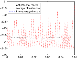
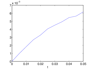
Figure 1. Convergence of the energy for problem (1.4) to that of (1.6) is a good way to keep track of the time-averaging, as well as a diagnostic tool for the computation. Here we show the differences of the energies (left) and the wave functions (right) between the fast potential model and time-averaged model. We take the time local average of $E^{\omega}(t)$ over $[t,t+0.005]$.

2. Numerical methods for nonlinear Schrödinger equations (1.4) and (1.6)

As we have shown in [2, 9, 10, 11] the time-splitting pseudo-spectral/Bloch-decomposition based pseudo-spectral methods works well for (non)linear Schrödinger equation (with periodic potential), thus we shall focus on these two kind of methods in this paper. We have shown that these two methods have spectral convergency in spatial discretization [2, 9, 10, 11].

2.1. Time-splitting spectral algorithm

We solve (1.4) or (1.6) by a classical time-splitting spectral scheme as follows [2, 11]:

Step 1. We solve the equation

(2.1) $$\,\mathrm{i}\partial_{t}u_{1}=-\,\Delta u_{1},$$

on a fixed time interval $\Delta t$, relying on the pseudo-spectral method. Thus we can get the value of $u_{1}$ at new time $t^{n+1}$ by

$$u^{n+1}_{1}=\left(e^{-\mathrm{i}\Delta t|\xi|^{2}}\hat{u}_{1}^{n}(\xi)\right)^{\vee},$$

here ‘$\wedge$’ and ‘$\vee$’ denote the Fourier and inverse Fourier transform respectively.

Let $\rho(t^{n+1},\boldsymbol{\rm{x}})=|u_{1}(t^{n+1},\boldsymbol{\rm{x}})|^{2}$, then we compute the Hartree potential $V_{Hartree}$ by

$$V_{Hartree}(t^{n+1},\boldsymbol{\rm{x}})=\left(\frac{1}{|\xi|^{2}}\hat{\rho}(t^{n+1},\xi)\right)^{\vee}.$$

Step 2. We solve the ordinary differential equation

(2.2) $$\,\mathrm{i}\partial_{t}u_{2}=\left(C_{1}V_{Hartree}+V(t,\boldsymbol{\rm{x}})-a|u_{2}|^{\sigma}\right)u_{2},\quad u_{2}(t^{n},\boldsymbol{\rm{x}})=u_{1}(t^{n+1},\boldsymbol{\rm{x}}),$$

on the same time-interval, here $V(t,\boldsymbol{\rm{x}})$ is given by (1.5) or (1.7). It is easy to check that in this step the density $\rho(t,\boldsymbol{\rm{x}})\equiv|u_{2}|^{2}(t,\boldsymbol{\rm{x}})$ and consequently the Hartree potential do not change in time, hence

$$u_{2}(t+\Delta t,\boldsymbol{\rm{x}})=u_{2}(t,\boldsymbol{\rm{x}})\,\exp\left({\displaystyle-\mathrm{i}\int_{t}^{t+\Delta t}\left(C_{1}V_{Hartree}(\boldsymbol{\rm{x}})+V(s,\boldsymbol{\rm{x}})-a\rho^{\frac{\sigma}{2}}(\boldsymbol{\rm{x}})\right)ds}\right)$$

with $\rho(\boldsymbol{\rm{x}})=|u_{1}(t^{n+1},\boldsymbol{\rm{x}})|^{2}$, $V_{Hartree}(x)=\left(\frac{1}{|\xi|^{2}}\hat{\rho}(\xi)\right)^{\vee}$.

The key is to calculate the oscillatory integral,

(2.3) $$\int_{t}^{t+\Delta t}\frac{1}{\left|\boldsymbol{\rm{x}}-b(s)\right|}ds\equiv\int_{t}^{t+\Delta t}\frac{1}{\left|\boldsymbol{\rm{x}}-e(s)\sin(2\pi\omega s)\right|}ds,$$

where $|\omega|\gg 1$, particularly due to the occurrence of the singularity in the kernel. Therefore, we use a regularization technique. For example, we could take

(2.4) $$\int_{t}^{t+\Delta t}\frac{1}{\left|\boldsymbol{\rm{x}}-b(s)\right|}ds\approx\int_{t}^{t+\Delta t}\Phi^{\eta}\left(\frac{1}{\left|\boldsymbol{\rm{x}}-b(s)\right|}\right)ds,$$

where

$$\Phi^{\eta}\left(\frac{1}{\left|\boldsymbol{\rm{x}}-b(s)\right|}\right)=\left(\frac{2}{\eta}\right)^{\frac{3}{2}}\int_{\mathbb{R}^{3}}e^{-2\pi\frac{|\boldsymbol{\rm{x}}-\boldsymbol{\rm{x}}^{\prime}|^{2}}{\eta}}\frac{1}{\left|\boldsymbol{\rm{x}}^{\prime}-b(s)\right|}d\boldsymbol{\rm{x}}^{\prime}.$$

In Section 4 we will discuss the stability with respect to perturbations of the potential.

The energies for two models are

(2.5) $$E^{\omega}(t):=\int_{\mathbb{R}^{3}}\left(|\nabla u^{\omega}|^{2}+\frac{C_{1}}{2}|\nabla V_{Hartree}^{\omega}|^{2}+cV^{\omega}|u^{\omega}|^{2}-a\frac{2}{\sigma+2}|u^{\omega}|^{\sigma+2}\right)d\boldsymbol{\rm{x}},$$

and

(2.6) $$E(t):=\int_{\mathbb{R}^{3}}\left(|\nabla u|^{2}+\frac{C_{1}}{2}|\nabla V_{Hartree}|^{2}+{c}\langle V\rangle|u|^{2}-a\frac{2}{\sigma+2}|u|^{\sigma+2}\right)d\boldsymbol{\rm{x}},$$

respectively. The total mass

(2.7) $$M(t):=\int_{\mathbb{R}^{3}}|u(t,\boldsymbol{\rm{x}})|^{2}d\boldsymbol{\rm{x}},$$

is conserved in both models.

2.2. Bloch-decomposition based time-splitting spectral algorithm

If we consider an external potential $V_{ext}\left(\boldsymbol{\rm{x}}\right)$ in the equation (1.1) [8, 14], we have

$$i\varepsilon\partial_{t}\psi=(i\varepsilon\nabla-A)^{2}\psi+V_{ext}(\boldsymbol{\rm{x}})\psi+c\frac{1}{|\boldsymbol{\rm{x}}|}\psi+C_{1}(|\cdot|^{-1}\ast|\psi|^{2})\psi-a|\psi|^{\sigma}\psi,$$

by the same transformation (1.2) and by fixing $\varepsilon=1$, we obtain the following equation

(2.8) $$i\partial_{t}u^{\omega}=-\Delta u^{\omega}+V_{ext}\left(\boldsymbol{\rm{x}}-b(t)\right)u^{\omega}+V^{\omega}u+C_{1}(|\cdot|^{-1}\ast|u^{\omega}|^{2})u^{\omega}-a|u^{\omega}|^{\sigma}u^{\omega},$$

and its time-averaged problem is

(2.9) $$i\partial_{t}u=-\Delta u+\langle V_{ext}\rangle u+\langle V\rangle u+C_{1}(|\cdot|^{-1}\ast|u|^{2})u-a|u|^{\sigma}u,$$

with

$$\langle V_{ext}\rangle(t,\boldsymbol{\rm{x}})=\displaystyle\int\limits_{-\frac{1}{2}}^{{\frac{1}{2}}}V_{ext}\left(\boldsymbol{\rm{x}}-e(t)\sin(2\pi s)\right)ds.$$

In particular, if we consider a case with an periodic potential $V_{\Gamma}\left(\boldsymbol{\rm{x}}\right)$ [8, 14], i.e. $V_{\Gamma}(\boldsymbol{\rm{y}})$ is periodic w.r.t to a regular lattice $\Gamma$,

$$V_{\Gamma}(\boldsymbol{\rm{y}}+\gamma)=V_{\Gamma}(\boldsymbol{\rm{y}}),\quad\forall\gamma\in\Gamma,\boldsymbol{\rm{y}}\in\mathbb{R}^{3},$$

the above two equations (2.8)–(2.9) become

(2.10) $$i\partial_{t}u^{\omega}=-\Delta u^{\omega}+V_{\Gamma}\left(\boldsymbol{\rm{x}}-b(t)\right)u^{\omega}+V^{\omega}u+C_{1}(|\cdot|^{-1}\ast|u^{\omega}|^{2})u^{\omega}-a|u^{\omega}|^{\sigma}u^{\omega},$$

and its time-averaged problem is

(2.11) $$i\partial_{t}u=-\Delta u+\langle V_{\Gamma}\rangle\left(t,\boldsymbol{\rm{x}}\right)u+\langle V\rangle u+C_{1}(|\cdot|^{-1}\ast|u|^{2})u-a|u|^{\sigma}u,$$

with

$$\langle V_{\Gamma}\rangle(t,\boldsymbol{\rm{x}})=\displaystyle\int\limits_{-\frac{1}{2}}^{{\frac{1}{2}}}V_{\Gamma}\left(\boldsymbol{\rm{x}}-e(t)\sin(2\pi s)\right)ds.$$

We solve (2.10) or (2.11) by using the Bloch-decomposition based time-splitting method, see [9, 10].

Step 1. We solve the equation

(2.12) $$\,\mathrm{i}\partial_{t}u_{1}=-\,\Delta u_{1}+V_{\Gamma}\left(t,\boldsymbol{\rm{x}}\right)u_{1},$$

on a fixed time interval $\Delta t$, relying on the Bloch-decomposition based pseudo-spectral method.

Let $\rho(t^{n+1},\boldsymbol{\rm{x}})=|u_{1}(t^{n+1},\boldsymbol{\rm{x}})|^{2}$, then we obtain the Hartree potential $V_{Hartree}$ by

$$V_{Hartree}\left(t^{n+1},\boldsymbol{\rm{x}}\right)=\left(\frac{1}{|\xi|^{2}}\hat{\rho}(t^{n+1},\xi)\right)^{\vee}.$$

Step 2. Then, we solve the ordinary differential equation

(2.13) $$\,\mathrm{i}\partial_{t}u_{2}=\left(C_{1}V_{Hartree}+V(t,\boldsymbol{\rm{x}})-a|u_{2}|^{\sigma}\right)u_{2},\quad u_{2}\left(t^{n},\boldsymbol{\rm{x}}\right)=u_{1}\left(t^{n+1},\boldsymbol{\rm{x}}\right),$$

on the same time-interval, here $V(t,\boldsymbol{\rm{x}})$ is given by (1.5) or (1.7). It is easy to check that in this step the density $\rho(t,\boldsymbol{\rm{x}})\equiv|u_{2}|^{2}(t,\boldsymbol{\rm{x}})$ and consequently the Hartree potential do not change in time, hence

$$u_{2}(t+\Delta t,\boldsymbol{\rm{x}})=u_{2}(t,\boldsymbol{\rm{x}})\,\exp\left({\displaystyle-\mathrm{i}\int_{t}^{t+\Delta t}\left(C_{1}V_{Hartree}(\boldsymbol{\rm{x}})+V(s,\boldsymbol{\rm{x}})-a\rho^{\frac{\sigma}{2}}(\boldsymbol{\rm{x}})\right)ds}\right)$$

with $\rho(\boldsymbol{\rm{x}})=\left|u_{1}(t^{n+1},\boldsymbol{\rm{x}})\right|^{2}$, $V_{Hartree}(x)=\left(\frac{1}{|\xi|^{2}}\hat{\rho}(\xi)\right)^{\vee}$.

Remark 2.1.

Certainly, if there is no lattice potential $V_{\Gamma}$, the above two algorithms are coincided with each other. But we must include the lattice potential $V_{\Gamma}$ when the interaction with laser or other lattice potenital are not eligible. We will see that the Bloch-decomposition based method is much more efficient in the case with lattice potential $V_{\Gamma}$ than the traditional pseudo-spectral method (cf. Fig. 16-17), i.e. we could use much larger mesh size than the traditional pseudo-spectral method to get the same accuracy.

3. Numerical results

3.1. Numerical experiments

3.1.1. Convergence to the time-averaged model

Example 3.1.

Here we set the semiclassical parameter $\varepsilon=1$, $e(t)=(0,0,1)^{T}$, $\sigma=\frac{2}{3}$, $a=50$, $C_{1}=20$, $c=1$. We compare the time-averaged model with the fast-potential model for different values of $\omega$. We choose appropriate constants $C_{1}$ and $c$ to make the two potential components in the energy comparable.

Table 1. Example 3.1: errors between two models vs frequency $\omega$.

$\omega$	5	10	20	40
$\|u-u^{\omega}\|_{L^{2}}$	1.1E-1	5.4E-2	2.9E-2	1.8E-2
convergence rate		1.0	0.9	0.7
$\|E-E^{\omega}\|_{L^{1}}$	7.1E-1	4.5E-1	2.9E-1	1.9E-1
convergence rate		0.6	0.6	0.6

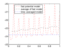
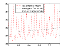
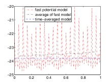
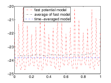
$\omega=5$                            $\omega=10$                           $\omega=20$                          $\omega=40$

Figure 2. Example 3.1: Comparison of the energies of two models with different $\omega$. Here we take the average of $E^{\omega}(t)$ over $[t,t+0.1]$.

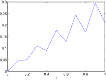
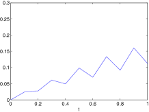
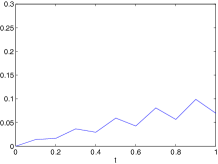
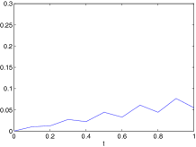
$\omega=5$                            $\omega=10$                           $\omega=20$                          $\omega=40$

Figure 3. Example 3.1: The relative distance between the wavefunctions of two models with different $\omega$: $\frac{\|u^{\omega}-u\|_{L^{2}}}{\|u\|_{L^{2}}}$.

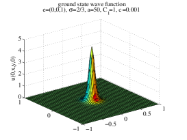
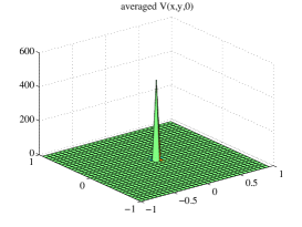
Initial datum $u_{0}(x,y,0)$                   $\overline{V}(x,y,0)$

Figure 4. Example 3.1: Graphs of the time-averaged model, the parameters are: $\varepsilon=1$, $e(t)=(0,0,1)^{T}$, $\sigma=\frac{2}{3}$, $a=50$, $C_{1}=1$, $c=0.001$. Our numerical results show the conservation of the energy $E(t)$ (given by (2.6)) and mass $M(t)$ (given by (2.7)) in both time-averaged model and fast-potential model.

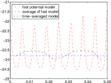
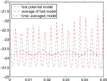
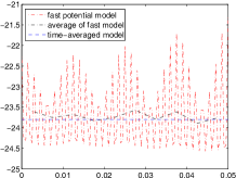
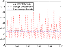
$\omega=80$                         $\omega=160$                         $\omega=320$                         $\omega=640$

Figure 5. Example 3.1: The distance between the energies of two models with larger $\omega$ vs. time. Here we take the average of $E^{\omega}(t)$ over $[t,t+0.005]$.

Remark 3.1.

From Figures 2–4, we can see that as $|\omega|\to\infty$, the average of the energy $E^{\omega}(t)$ converges to the energy $E(t)$ of time-averaged model. The corresponding wave-function $u^{\omega}(t,\boldsymbol{\rm{x}})$ also converges to $u(t,\boldsymbol{\rm{x}})$ at least in $L^{2}$-norm. Figure 4 also shows the conservation of $E(t)$ and $M(t)$.

3.1.2. Blow-up tests

Example 3.2.

Here we consider an example with $\varepsilon=1$, $e(t)=(0,0,1)^{T}$, $a=50$, $C_{1}=100$, $c=0.1$. We start the time-averaged model from a ground state for $\sigma=2/3$ (cf. plot (a) in Fig. 6). Then we consider (1.4) with a mass supercritical power-type nonlinearity, i.e. $\sigma>4/3$, we analyse the blow-up of the norm

(3.1) $$\|\nabla u\|_{L^{2}}=\left(\int_{\mathbb{R}^{3}}|\nabla u(t,\boldsymbol{\rm{x}})|^{2}d\boldsymbol{\rm{x}}\right)^{1/2}.$$

In Fig. 6–7, we can see that the blow-up time decreases as $\sigma$ increases.

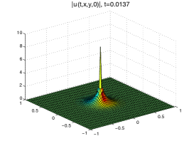
Initial datum $u_{0}(x,y,0)$                   $|u(t,x,y,0)|$

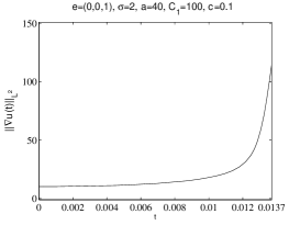
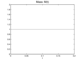
$\|\nabla u\|_{L^{2}}$ (given by (3.1))               $M(t)$ (given by (2.7))

Figure 6. Example 3.2: Graphs of the time-averaged model, the parameters are: $\varepsilon=1$, $e(t)=(0,0,1)^{T}$, $\sigma=2$, $a=50$, $C_{1}=100$, $c=0.1$. Blow-up case.

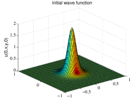
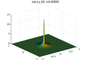
Initial datum $u_{0}(x,y,0)$                   $|u(t,x,y,0)|$

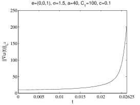
$\|\nabla u\|_{L^{2}}$ (given by (3.1))               $M(t)$ (given by (2.7))

Figure 7. Example 3.2: Graphs of the time-averaged model, the parameters are: $\varepsilon=1$, $e(t)=(0,0,1)^{T}$, $\sigma=1.5$, $a=50$, $C_{1}=100$, $c=0.1$. Blow-up case.

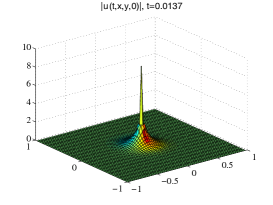
$u(t,x,y,0)$                        $\|\nabla u\|_{L^{2}}$ (given by (3.1))

Figure 8. Example 3.2: Graphs of the fast-potential model, the parameters are: $\varepsilon=1$, $e(t)=(0,0,1)^{T}$, $\sigma=2$, $a=50$, $C_{1}=100$, $c=0.1$, $\omega=10^{4}$. Blow-up case.

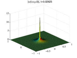
$u(t,x,y,0)$                        $\|\nabla u\|_{L^{2}}$ (given by (3.1))

Figure 9. Example 3.2: Graphs of the fast-potential model, the parameters are: $\varepsilon=1$, $e(t)=(0,0,1)^{T}$, $\sigma=1.5$, $a=50$, $C_{1}=100$, $c=0.1$, $\omega=10^{4}$.

Comparing the $L^{2}$ norms of the gradient of the wave-function for the time averaged model and the fast model in the blow up test we can see that they are very similar in the super-critical case (cf. Figures 8–9 and Figures 6–7). They exhibit more differences in the subcritical case (see Fig. 10–11).

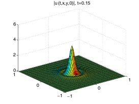
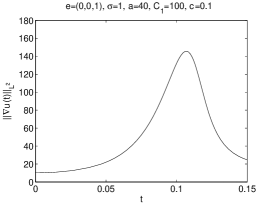
$|u(t,x,y,0)|_{t=0.15}|$                   $|u(t,x,y,0)|_{t=0.11}|$                  $\|\nabla u\|_{L^{2}}$ (given by (3.1))

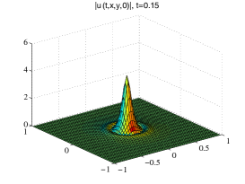
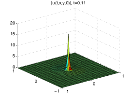
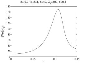
$|u(t,x,y,0)|_{t=0.15}|$                   $|u(t,x,y,0)|_{t=0.11}|$                  $\|\nabla u\|_{L^{2}}$ (given by (3.1))

Figure 10. Example 3.2: Graphs of the fast-potential model (first line) and time-averaged model (second line), the parameters are: $\varepsilon=1$, $e(t)=(0,0,1)^{T}$, $\sigma=1$, $a=50$, $C_{1}=100$, $c=0.1$, $\omega=10^{4}$.

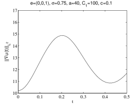
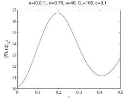
$\|\nabla u^{\omega}\|_{L^{2}}$ (given by (3.1))            $\|\nabla u\|_{L^{2}}$ (given by (3.1))

Figure 11. Example 3.2: Graphs of the fast-potential model (left) and time-averaged model (right), the parameters are: $\varepsilon=1$, $e(t)=(0,0,1)^{T}$, $\sigma=0.75$, $a=50$, $C_{1}=100$, $c=0.1$, $\omega=10^{4}$.

Furthermore, from Figures 12–13, we can see that the Coulomb potential significantly impacts the wave packet at the early stage. This becomes particularly clear with slower blow-up and smaller frequency $\omega$.

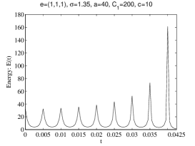
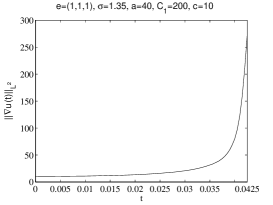
$E(t)$ (given by (2.5))                $\|\nabla u\|_{L^{2}}$ (given by (3.1))                    $|u(t,x,y,0)|_{t=0}|$

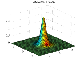
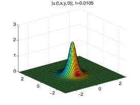
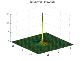
$|u(t,x,y,0)|_{t=0.006}|$                  $|u(t,x,y,0)|_{t=0.0105}|$                  $|u(t,x,y,0)|_{t=0.0425}|$

Figure 12. Example 3.2: Graphs of the fast-potential model, the parameters are: $\varepsilon=1$, $e(t)=(1,1,1)^{T}$, $\sigma=1.35$, $a=40$, $C_{1}=200$, $c=10$, $\omega=10^{2}$.

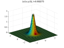
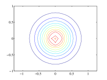
$|u(0,x,y,0)|$             $\|\nabla u\|_{L^{2}}$ (given by (3.1))      $|u(t,x,y,0)|_{t=0.002275}|$            contour plot

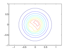
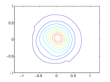
$|u(t,x,y,0)|_{t=0.00819}|$             contour plot             $|u(t,x,y,0)|_{t=0.020475}|$              contour plot

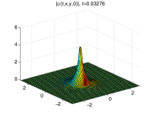
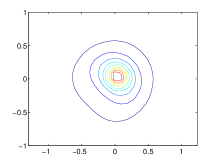
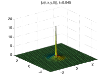
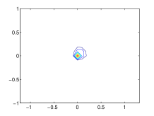
$|u(t,x,y,0)|_{t=0.03276}|$              contour plot              $|u(t,x,y,0)|_{t=0.045}|$                contour plot

Figure 13. Example 3.2: Graphs of the fast-potential model, the parameters are: $\varepsilon=1$, $e(t)=(-1,-1,-1)^{T}$, $\sigma=1.35$, $a=40$, $C_{1}=200$, $c=10$, $\omega=5$.

3.1.3. Interaction of the magnetic field with the particle

Example 3.3.

Here we are interested in the patterns of interaction of the magnetic field with the particle, especially when a particle is shot towards the field, and scattered by it. We set $e=(0,0,1)^{T}$ in eq. (1.5), and choose an initial datum of the form

$$u_{0}(\boldsymbol{\rm{x}})=e^{-4|\boldsymbol{\rm{x}}-(1,1,0)^{T}|^{2}+i(x_{1}-x_{2})},\quad\mbox{ for }\boldsymbol{\rm{x}}=(x_{1},x_{2},x_{3})^{T}.$$

In this example, we add a harmonic trap potential

$$V(\boldsymbol{\rm{x}})=50|\boldsymbol{\rm{x}}|^{2},$$

i.e. the equation in (1.4) becomes

(3.2) $$i{\partial}_{t}u^{\omega}=-\Delta u^{\omega}+V\left(\boldsymbol{\rm{x}}-b(t)\right)u^{\omega}+V^{\omega}u^{\omega}+C_{1}(|\cdot|\ast|u^{\omega}|^{2})u^{\omega}-a|u^{\omega}|^{\sigma}u^{\omega}$$

The results are shown in Figure 14. We can see that the wave packet moves under the interaction with the trap $V(\boldsymbol{\rm{x}})$.

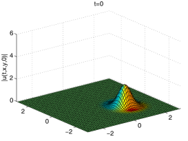
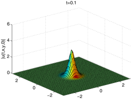
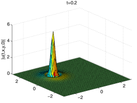
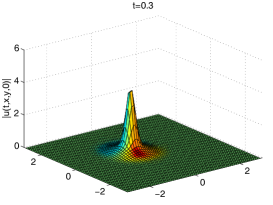
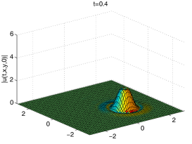
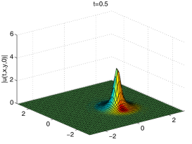
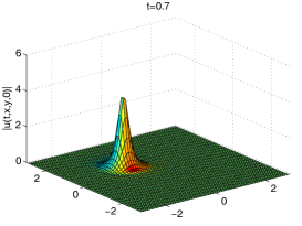
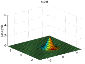
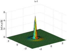
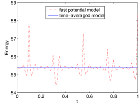
Figure 14. Example 3.3: (fast-potential model), the parameters are: $\varepsilon=1$, $e(t)=(0,0,1)^{T}$, $\sigma=\frac{2}{3}$, $a=50$, $C_{1}=20$, $c=1$, $\omega=10^{2}$.

3.1.4. Time-dependent vectors $e(t)$

Example 3.4.

We consider a time-dependent vector $e(t)=(-1,-1,-1)\sin 2\pi t$ in eq. (1.5), and an initial datum of the form

$$u_{0}(x)=e^{-4|\boldsymbol{\rm{x}}|^{2}}.$$

The results are shown in Figure 15. As $e(t)$ is slowly varying in time, its effects are not very pronounced except when $e(t)$ is close to 0.

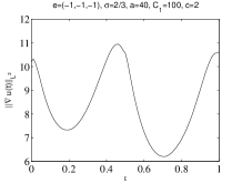
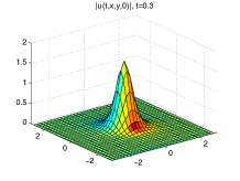
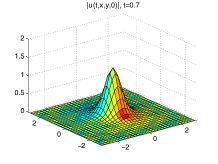
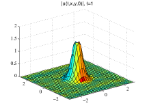
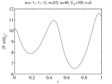
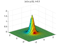
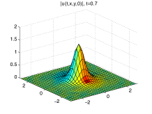
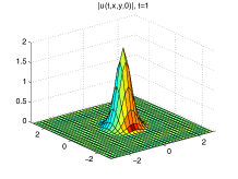
Figure 15. Example 3.4: Graphs of the example 3.4 for fast-potential model (first line) and time-averaged model (second line), the parameters are: $\varepsilon=1$, $e(t)=(-1,-1,-1)^{T}\sin 2\pi t$, $\sigma=\frac{2}{3}$, $a=40$, $C_{1}=100$, $c=2$, $\omega=10^{2}$.

3.1.5. Interaction with periodic lattice

Example 3.5.

Finally, we consider a case with periodic lattice, i.e. the equation in (1.4) becomes

(3.3) $$i{\partial}_{t}u^{\omega}=-\Delta u^{\omega}+V^{\omega}u^{\omega}+V_{\Gamma}\left(\boldsymbol{\rm{x}}-b(t)\right)u^{\omega}+C_{1}(|\cdot|^{-1}\ast|u^{\omega}|^{2})u^{\omega}-a|u^{\omega}|^{\sigma}u^{\omega},$$

and its time-averaged problem is

(3.4) $$i{\partial}_{t}u=-\Delta u+\langle V\rangle u+\langle V_{\Gamma}\rangle u+C_{1}(|\cdot|^{-1}\ast|u|^{2})u-a|u|^{\sigma}u.$$

We also take the initial datum of the form

$$u_{0}(x)=e^{-4|\boldsymbol{\rm{x}}|^{2}}.$$

Here $V_{\Gamma}(\boldsymbol{\rm{y}})$ is periodic w.r.t to a regular lattice $\Gamma$,

$$V_{\Gamma}(\boldsymbol{\rm{y}}+\gamma)=V_{\Gamma}(\boldsymbol{\rm{y}}),\quad\forall\gamma\in\Gamma,\ \boldsymbol{\rm{y}}\in\mathbb{R}^{3}.$$

For sake of simplicity, we choose

$$V_{\Gamma}(\boldsymbol{\rm{y}})=\sum_{l=1}^{3}\sin^{2}(\omega_{l}y_{l}),\quad\mbox{ for }\boldsymbol{\rm{y}}=(y_{1},y_{2},y_{3})^{T}\in\mathbb{R}^{3},$$

with $\omega_{1}=\omega_{2}=\omega_{3}=2\pi$.

The results are shown in Figures 16-17. We can see the interaction between the lattice potential and the wave packet. Certainly, the wave function of the fast model is more peaked than the solution of the time-averaged model. From these figures, we can also find that the Bloch-decomposition based algorithm is more efficient than traditional pseudo-spectral method in this case.

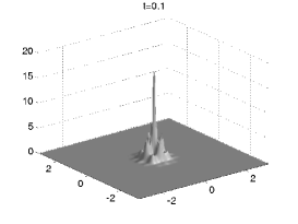
Figure 16. Graphs of $|u^{\omega}(t,x,y,0)|^{2}$ and $|u(t,x,y,0)|^{2}$ of the example 3.5 for fast-potential model (left $\omega=80$, middle $\omega=160$) and time-averaged model (right) by our Bloch-decomposition based algorithm given in section 2.2, the parameters are: $\varepsilon=\frac{1}{8}$, $e(t)=(0,0,1)^{T}$, $\sigma=\frac{2}{3}$, $a=1$, $C_{1}=1$, $c=2$, mesh size $h=\frac{1}{128}$.

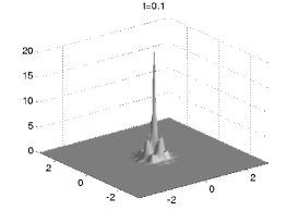
Figure 17. Graphs of $|u(t,x,y,0)|^{2}$ of the example 3.5 for fast-potential model by the typical pseudo-spectral method given in section 2.1 with $\omega=160$, left: mesh size $h=\frac{1}{128}$, right: $h=\frac{1}{1024}$.

4. Stability estimate

In this Section we present the analytical results needed in order to rigorously justify the approximation used in Section 2. Because of the singularities of the Coulomb potential, we use a mollified version in the numerical simulation. Here we discuss the additional errors introduced by the smoothing.

In order to avoid technicalities we only state a Proposition which shows that equation (1.4) is stable under perturbations of the potential. The proof is indeed quite standard, as similar results are well known in the literature, see below for the references. The proof of stability of equation (1.4) with respect to perturbations of the potential is done by adapting in a straightforward way the local well-posedness result. For furhter details we refer the reader to [12], [4] Section 4.

Theorem 4.1.

Let $V,\tilde{V}$ be two potentials such that $V,\tilde{V}\in L^{\infty}(\mathbb{R};L^{\frac{3}{1+3\delta}}(\mathbb{R}^{3})+L^{\frac{3}{1-3\delta}}(\mathbb{R}^{3}))$, $\nabla V,\nabla\tilde{V}\in L^{\infty}(\mathbb{R};L^{\frac{3}{2+3\delta}}(\mathbb{R}^{3})+L^{\frac{3}{2-3\delta}}(\mathbb{R}^{3}))$, for some $\delta>0$ small. Let $u,\tilde{u}$ be the solutions of the Cauchy problems

$$\left\{\begin{aligned} &i\partial_{t}u=-\Delta u+Vu+C_{1}(|\cdot|^{-1}\ast|u|^{2})u-a|u|^{\sigma}u\\ &u(t,\boldsymbol{\rm{x}})\big{|}_{t=0}=u_{0}(\boldsymbol{\rm{x}}),\end{aligned}\right.$$

with the potential $V$ and respectively with $V$ replaced by $\tilde{V}$, and initial data $u_{0}$ and, respectively $\tilde{u}_{0}\in H^{1}(\mathbb{R}^{3})$, respectively. Let $0<T<\min\{T_{max},\tilde{T}_{max}\}$, where $T_{max},\tilde{T}_{max}$ are the maximal existence times for $u,\tilde{u}$, respectively. Then, for any admissible pair $(q,r)$, we have

(4.1) $$\|u-\tilde{u}\|_{L^{q}((0,T);W^{1,r}(\mathbb{R}^{3}))}\leq C\left(\|u_{0}-\tilde{u}_{0}\|_{H^{1}}+\|V-\tilde{V}\|_{L^{\infty}_{t}(L^{\frac{3}{1+3\delta}}_{x}+L^{\frac{3}{1-3\delta}}_{x})}+\|\nabla(V-\tilde{V})\|_{L^{\infty}_{t}(L^{\frac{3}{2+3\delta}}_{x}+L^{\frac{3}{2-3\delta}}_{x})}\right).$$

5. Conclusion

In this paper, we propose the time-splitting (Bloch-decomposition based) pseudo-spectral methods to simulate the XFEL Schrödinger equation (with and without periodic potential). Our simulation results go far beyond known analytical results [1]. In particular we demonstrate numerically that the time-averaging procedure works in mass supercritical/energy subcritical cases, even up to blow-up time. Moreover, we show numerically that the energy of the oscillatory problem converges weakly in time to the energy of the time averaged problem (which is constant when the vector $e(t)$ is not dependent on time). Also, we demonstrate the impact of external trapping potentials and periodic lattice potentials on the electron beam wave function and numerically verify the time average procedure in those cases.

References

- [1] P. Antonelli, A. Athanassoulis, H. Hajaiej, and P. Markowich, On the XFEL Schrödinger equation: highly oscillatory magnetic potentials and time averaging, preprint, arXiv:1209.6089v1.
- [2] W. Z. Bao, S. Jin, and P. Markowich, On time-splitting spectral approximations for the Schrödinger equation in the semiclassical regime, J. Comp. Phys. 175 (2002), 487–524.
- [3] J. D. Brock, Watching Atoms Move, Science 315 (2007), 609 –610.
- [4] T. Cazenave, Semilinear Schrödinger Equations. Courant Lecture Notes in Mathematics vol. 10, New York University, Courant Institute of Mathematical Sciences, AMS, 2003.
- [5] T. Cazenave, M. Scialom, A Schrödinger equation with time-oscillating nonlinearity, Rev. Mat. Univ. Complut. Madrid 23 (2010), 321–339.
- [6] H. N. Chapman et al., Femtosecond time-delay X-ray holography, Nature 448 (2007), 676–679.
- [7] A. Fratalocchi and G. Ruocco, Single-molecule imaging with x-ray free electron lasers: Dream or reality? Phys. Rev. Lett. 106 (2011), 105504.
- [8] D. M. Fritz et al., Ultrafast Bond Softening in Bismuth: Mapping a Solid’s Interatomic Potential with X-rays, Science 315 (2007), 633–636.
- [9] Z. Huang, S. Jin, P. Markowich, and C. Sparber, A Bloch decomposition based split-step pseudo spectral method for quantum dynamics with periodic potentials, SIAM J. Sci. Comput. 29 (2007), 515–538.
- [10] Z. Huang, S. Jin, P. Markowich, and C. Sparber, Numerical simulation of the nonlinear Schrödinger equation with multi-dimensional periodic potentials, Multiscale Model. Simul. 7 (2008), 539–564.
- [11] Z. Huang, S. Jin, P. Markowich, C. Sparber and C. Zheng, A Time-splitting spectral scheme for the Maxwell-Dirac system, J. Comput. Phys. 208 (2005), 761–789.
- [12] T.Kato, On nonlinear Schrödinger equations, Ann. Inst. Henri Poincaré 46, 1 (1987), 113–129.
- [13] M. Keel and T. Tao, Endpoint Strichartz Estimates. Amer. J. Math. 120 (1998), 955–980.
- [14] B. W. J. McNeil and N. R. Thompson, X-ray free-electron lasers, Nature Photonics 4 (2010), 814–821.
- [15] R. Neutze, et al, Potential for biomolecular imaging with femtosecond X-ray pulses, Nature 406 (2000), 752–757.