DESY 14-087 IFJPAN-IV-2014-10 LPN 14-077 Calculation of QCD NLO Splitting Functions in the light-cone gauge: a new regularization prescription

Abstract

We report on the progress in calculating NLO DGLAP splitting functions for $x<1$ using the New Principal Value prescription, which is a modification of the standard Principal Value approach proposed by Curci, Furmanski and Petronzio in 1980. The new prescription reproduces the standard results on the inclusive (integrated) level, but simplifies individual contributions and restricts the cancellations between real and virtual diagrams which makes it useful for Monte Carlo simulations.

12.38.-t, 12.38.Bx, 12.38.Cy

1 Introduction

In QCD in addition to the ultra-violet (UV) singularities also mass singularities appear. Mass singularities can be further divided into infra-red (IR) and collinear ones. By analogy with the UV divergences, which rule the evolution of the strong coupling constant $\alpha_{\mathrm{s}}$, the collinear divergences rule the evolution of parton distribution functions, $f_{i}$. This evolution is governed by the DGLAP equations [1, 2, 3] which read:

$$\frac{\partial}{\partial\ln\mu^{2}}f_{i}\left(x,\mu^{2}\right)=\sum_{j=g,q,\bar{q}}\int_{x}^{1}\frac{\mathrm{d}z}{z}P_{ij}\left(z,\alpha_{\mathrm{s}}(\mu^{2})\right)f_{j}\Bigl{(}\frac{x}{z},\mu^{2}\Bigr{)}\text{,}$$ (1)

where $\mu$ is the factorization scale, $i,j=g,q,\bar{q}$ goes over all types of partons, and $P_{ij}\left(x,\alpha_{\mathrm{s}}\right)$ are the DGLAP splitting functions (evolution kernels).

As opposed to parton distributions, the evolution kernels can be calculated perturbatively and we can write their expansion in powers of $\alpha_{\mathrm{s}}$ as

$$P_{ij}\left(x,\alpha_{\mathrm{s}}(\mu^{2})\right)=\frac{\alpha_{\mathrm{s}}}{2\pi}P_{ij}^{(0)}\left(x\right)+\Bigl{(}\frac{\alpha_{\mathrm{s}}}{2\pi}\Bigr{)}^{2}P_{ij}^{(1)}\left(x\right)+\operatorname{\mathcal{O}}(\alpha_{\mathrm{s}}^{3})\text{.}$$ (2)

The lowest $\operatorname{\mathcal{O}}(\alpha_{\mathrm{s}})$ splitting functions $P_{ij}^{(0)}(x)$ are known for about forty years, e.g. see [1, 4]. Later, the $\operatorname{\mathcal{O}}(\alpha_{\mathrm{s}}^{2})$ splitting functions were calculated with the help of two independent methods: 1) the operator product expansion (OPE) [5, 6] and 2) the method of Curci, Furmanski, and Petronzio (CFP) [4, 7] which is based on factorization properties of mass singularities in the light-cone gauge [8]. The latest, state-of-the-art results for the $\operatorname{\mathcal{O}}(\alpha_{\mathrm{s}}^{3})$ space-like splitting functions were obtained with OPE approach in [9, 10], and approximate results for the $\operatorname{\mathcal{O}}(\alpha_{\mathrm{s}}^{3})$ time-like splitting functions are available in [11, 12].

Such impressive results obtained with the OPE method are caused by its technical simplicity compared to the CFP approach. The latter method operates in the physical momentum space and uses light-cone gauge which introduces additional complications due to the axial-type denominator $1/(ln)$, where $n$ is a light-cone reference vector. Despite of this complication, the CFP method provides a more clear physical picture of the collinear limit, i.e. generalized ladder expansion [8].

This fact is used to build the first fully next-to-leading-order (i.e. $\operatorname{\mathcal{O}}(\alpha_{\mathrm{s}}^{2})$) parton shower Monte Carlo generator [13, 14, 15] (with NLO corrections included in both the hard matrix element and the shower itself). Construction of such a NLO shower, however, requires the knowledge about the $\operatorname{\mathcal{O}}(\alpha_{\mathrm{s}}^{2})$ splitting functions at the exclusive, unintegrated, level. It means that, in addition to the known dependence on the longitudinal momentum fraction $x$, the dependence on the transverse momentum variable should be also known. Because of this, the use of the OPE method becomes more complicated in comparison to the CFP approach.

Moreover, the $\operatorname{\mathcal{O}}(\alpha_{\mathrm{s}}^{2})$ splitting functions calculated in the standard CFP approach, that are available in the literature [4, 18, 19], are also not well suited for the purpose of Monte Carlo simulations of parton cascades. First, the literature provides mostly the inclusive splitting functions (after integration over the final state momenta). Second, in the classic CFP approach there are cancellations between real and virtual contributions that are realized through cancellation of dimensional $\epsilon$ poles. This is incompatible with the Monte Carlo parton shower algorithms, and motivates modification of the CFP prescription [21] and recalculation of the $\operatorname{\mathcal{O}}(\alpha_{\mathrm{s}}^{2})$ evolution kernels.

We already started to calculate the NLO DGLAP kernels in the modified scheme. For the first time the new approach was used to calculate the real contributions to the non-singlet splitting function [20]. After that, we proceed with one-loop virtual contributions [22] and would like to report on these results in this paper.

2 The New Principal Value Prescription

Contributions to the NLO splitting functions for $x<1$ come from two types of topologies, further referred to as real – with two final-state momenta; and virtual – with one virtual and one final-state momentum. At the inclusive level these two cases can be added together since all, real and virtual, momenta are integrated out and only $x$-dependence is left. With more detailed analysis of the standard calculation procedure [19] one can find that $1/\epsilon^{3}$ terms cancel between these two contributions, while, as expected, terms $1/\epsilon^{2}$ and lower survive. Existence of $1/\epsilon^{3}$ poles is a serious problem for Monte-Carlo application of splitting functions, since at the exclusive level the real and virtual contributions are defined in different phase spaces, two- and one-particle ones respectively. Therefore, the contributions can not be easily added in order to cancel higher-order poles in $\epsilon$ and to make splitting functions finite in $\epsilon\to 0$ limit at the exclusive level. Fortunately, this issue can be resolved with a modification to the standard PV regularization prescription for the light-cone singularities, which we proposed in [21, 22].

In the standard approach the PV regularization is applied only to the axial denominator in the gluon propagator at the level of the Feynman rules:

$$g^{\mu\nu}-\frac{l^{\mu}n^{\nu}+l^{\nu}n^{\mu}}{ln}\rightarrow g^{\mu\nu}-\left(l^{\mu}n^{\nu}+l^{\nu}n^{\mu}\right)\frac{ln}{(ln)^{2}+\delta^{2}(pl)},$$ (3)

where $\delta$ is an infinitesimal regulator and $p$ is an external reference momentum. However, there are also singularities in the $l_{+}=(ln)/(pn)$ variable originating from the phase space parametrization or the Feynman part of gluon propagator and in the standard approach these are regularized in a dimensional manner. In the New Principal Value (NPV) prescription [21] the PV regularization is used to regularize all the singularities in the $l^{+}$ variable, regardless of their origin. For instance, we do the following replacement:

$$d^{m}l\,l_{+}^{\epsilon-1}\rightarrow d^{m}l\,\frac{l_{+}}{l_{+}^{2}+\delta^{2}}\left(1+\epsilon\ln l_{+}+\epsilon^{2}\frac{1}{2}\ln^{2}l_{+}+\dots\right)$$ (4)

in the entire integrand.

When the new prescription is used, there is one technical point we would like to underline. As opposed to the standard techniques of calculating loop integrals, where we introduce e.g. the Feynman parameters and integrate over them at the very end of the calculation, in the NPV prescription we perform the integration over the “plus” component ($l_{+}$) as the last one.

In the NPV prescription singularities appearing as double $\epsilon$ poles (before integration over scale, or in the case of virtual graphs before integration over final state momentum) are changed to double logarithms in the regulator $\delta$ or combination of single logarithms and single poles. For example, if we consider a three-point Feynman integral (kinematical set-up: $p^{2}=(p-q)^{2}=0,\;q^{2}<0$) in the standard CFP approach, we have:

$$J_{3}^{\mathrm{F}}=\int\frac{\mathrm{d}^{m}l}{(2\pi)^{m}}\frac{1}{l^{2}(q-l)^{2}(p-l)^{2}}=\frac{i}{(4\pi)^{2}\lvert q^{2}\rvert}\left(\frac{4\pi}{\lvert q^{2}\rvert}\right)^{-\epsilon}\Gamma(1-\epsilon)\left(-\frac{1}{\epsilon^{2}}+\frac{\pi^{2}}{6}\right),$$ (5)

and in the NPV prescription it is given by:

$$\begin{split}J_{3}^{\mathrm{F}}=&\frac{i}{(4\pi)^{2}\lvert q^{2}\rvert}\left(\frac{4\pi}{\lvert q^{2}\rvert}\right)^{-\epsilon}\Gamma(1-\epsilon)\bigg{(}-\frac{2I_{0}+\ln(1-x)}{\epsilon}-4I_{1}+2I_{0}\ln(1-x)+\frac{\ln^{2}(1-x)}{2}\bigg{)}.\end{split}$$ (6)

In this example we can explicitly see how the $\epsilon$ pole is replaced by the geometrical regulator which can be actually implemented in a Monte Carlo program. It is also important that in most cases the singularities regularized by $I_{0}$ and $I_{1}$ cancel separately between the real and virtual contributions.

3 NLO Splitting Functions

In this section, we present a few selected results obtained in the NPV scheme. Namely, we show all contributions to the inclusive splitting function $P_{qq}$ and selected contributions to the $P_{gg}$ one. This is enough to demonstrate explicitly that the NPV prescription leads to the same inclusive splitting functions as the standard PV scheme, but at the same time can be used at the exclusive level for Monte Carlo simulations in four dimensions. All the contributing graphs are shown in Fig. 1.

(c): $C_{f}^{2}-\frac{1}{2}C_{f}C_{a}$

(a) *

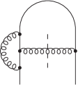
(d-qq): $\frac{1}{2}C_{f}C_{a}$

(b) *

(d-gg): $C_{a}^{2}$

(c) *

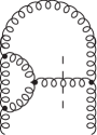
      (e): $C_{f}^{2}$

(d) *

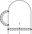
(f): $C_{f}C_{a}$

(e) *

(g): $C_{f}T_{f}$

(f) *

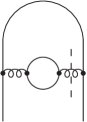
Figure 1: Virtual graphs contributing to the NLO splitting function $P_{qq}$ and one contribution to the $P_{gg}$ kernel.

Inclusive splitting functions are presented in Tables 1–2, where in the ‘virt’ column we provide contributions with one cut line, in the ‘real’ column – with two cut lines, and in ‘sum’ column – their sum. This allows for comparison of the results in NPV prescription with already known results in the PV prescription [4, 18, 19] and demonstrates the correctness of the proposed approach. The results in the ‘virt’ columns can be calculated with the help of the Axiloop package [23] and are available in [22, 21], the real contributions were calculated in [20]. The column ‘sum’ equals to the sum of the corresponding ‘virt’ and ‘real’ columns and is in full agreement with the known results, e.g. [18, 19].

	(d-qq)			(d-gg)			(c)
	virt	real	sum	virt	real	sum	virt	real	sum
Double Poles
$p_{qq}$	$-6$	$0$	$-6$	$-22/3$	$0$	$-22/3$	$-6$	$0$	$-6$
$p_{qq}\;\ln{x}$	$4$	$0$	$4$	$4$	$0$	$4$	$4$	$0$	$4$
$p_{qq}\;\ln(1-x)$	$8$	$0$	$8$	$4$	$0$	$4$	$0$	$0$	$0$
$p_{qq}\;I_{0}$	$16$	$0$	$16$	$12$	$0$	$12$	$8$	$0$	$8$
Single Poles
$p_{qq}$	$-7$	$-4$	$-11$	$-134/9$	$-4$	$-170/9$	$-7$	$0$	$-7$
$p_{qq}\;\ln{x}$	$0$	$-3/2$	$-3/2$	$0$	$-11/3$	$-11/3$	$0$	$-3/2$	$-3/2$
$p_{qq}\;\ln(1-x)$	$-3$	$8$	$5$	$-22/3$	$8$	$2/3$	$-3$	$0$	$-3$
$p_{qq}\;\ln^{2}{x}$	$2$	$-1$	$1$	$4$	$-2$	$2$	$2$	$-1$	$1$
$p_{qq}\;\ln{x}\ln(1-x)$	$2$	$4$	$6$	$4$	$4$	$8$	$2$	$0$	$2$
$p_{qq}\;\ln^{2}(1-x)$	$4$	$-2$	$2$	$4$	$-2$	$2$	$0$	$0$	$0$
$p_{qq}\;\>\mathrm{Li_{2}}(1)$	$8$	$-2$	$6$	$12$	$-2$	$10$	$4$	$0$	$4$
$p_{qq}\;\>\mathrm{Li_{2}}(1-x)$	$-2$	$2$	$0$	$0$	$0$	$0$	$2$	$-2$	$0$
$1/x$	$0$	$0$	$0$	$0$	$-22/3$	$-22/3$	$0$	$0$	$0$
$1$	$-3$	$2$	$-1$	$0$	$25/3$	$25/3$	$-3$	$-8$	$-11$
$x$	$2$	$-1$	$1$	$-1/3$	$-24/3$	$-25/3$	$4$	$7$	$11$
$x^{2}$	$0$	$0$	$0$	$0$	$22/3$	$22/3$	$0$	$0$	$0$
$1/x\ln{x}$	$0$	$0$	$0$	$0$	$-11/3$	$-11/3$	$0$	$0$	$0$
$\ln{x}$	$2$	$1/2$	$5/2$	$0$	$-23/6$	$-23/6$	$2$	$-7/2$	$-3/2$
$x\ln{x}$	$-2$	$1/2$	$-3/2$	$0$	$-23/6$	$-23/6$	$-2$	$-7/2$	$-11/2$
$x^{2}\ln{x}$	$0$	$0$	$0$	$0$	$-11/3$	$-11/3$	$0$	$0$	$0$
$(1-x)\;\ln(1-x)$	$4$	$0$	$4$	$0$	$0$	$0$	$0$	$0$	$0$
Single Spurious Poles
$p_{qq}\;I_{0}$	$0$	$8$	$8$	$0$	$8$	$8$	$0$	$0$	$0$
$p_{qq}\;I_{0}\ln{x}$	$4$	$4$	$8$	$8$	$4$	$12$	$4$	$0$	$4$
$p_{qq}\;I_{0}\ln(1-x)$	$12$	$-4$	$8$	$16$	$-4$	$12$	$4$	$0$	$4$
$p_{qq}\;I_{1}$	$-12$	$4$	$-8$	$-16$	$4$	$-12$	$-4$	$0$	$-4$
$(1-x)\;I_{0}$	$8$	$0$	$8$	$0$	$0$	$0$	$4$	$0$	$4$

Table 1: Contributions to the inclusive splitting functions $P_{qq}$ and $P_{gg}$ from the graphs (d-qq), (d-gg), and (c) in the NPV prescription.

	(e)	(f)			(g)
	virt	virt	real	sum	virt	real	sum
Double Poles
$p_{qq}$	$6$	$44/3$	$-22/3$	$22/3$	$-8/3$	$4/3$	$-4/3$
$p_{qq}\;\ln{x}$	$-8$	$0$	$0$	$0$	$0$	$0$	$0$
$p_{qq}\;\ln(1-x)$	$0$	$-16$	$8$	$-8$	$0$	$0$	$0$
$p_{qq}\;I_{0}$	$-8$	$-16$	$8$	$-8$	$0$	$0$	$0$
Single Poles
$p_{qq}$	$7$	$0$	$103/9$	$103/9$	$0$	$-10/9$	$-10/9$
$p_{qq}\;\ln{x}$	$0$	$0$	$11/3$	$11/3$	$0$	$-2/3$	$-2/3$
$p_{qq}\;\ln(1-x)$	$3$	$22/3$	$-34/3$	$-4$	$-4/3$	$4/3$	$0$
$p_{qq}\;\ln^{2}{x}$	$-2$	$0$	$0$	$0$	$0$	$0$	$0$
$p_{qq}\;\ln{x}\ln(1-x)$	$-4$	$0$	$-4$	$-4$	$0$	$0$	$0$
$p_{qq}\;\ln^{2}(1-x)$	$0$	$-8$	$6$	$-2$	$0$	$0$	$0$
$p_{qq}\;\>\mathrm{Li_{2}}(1)$	$-4$	$0$	$-4$	$-4$	$0$	$0$	$0$
$p_{qq}\;\>\mathrm{Li_{2}}(1-x)$	$0$	$0$	$0$	$0$	$0$	$0$	$0$
$\phantom{(}1-x$	$3$	$22/3$	$-4$	$10/3$	$-4/3$	$0$	$-4/3$
$(1-x)\;\ln{x}$	$-4$	$0$	$0$	$0$	$0$	$0$	$0$
$(1-x)\;\ln(1-x)$	$0$	$-8$	$4$	$-4$	$0$	$0$	$0$
$\phantom{(}1+x$	$0$	$0$	$0$	$0$	$0$	$0$	$0$
$(1+x)\;\ln{x}$	$0$	$0$	$0$	$0$	$0$	$0$	$0$
Single Spurious Poles
$p_{qq}\;I_{0}$	$0$	$0$	$-4$	$-4$	$0$	$0$	$0$
$p_{qq}\;I_{0}\ln{x}$	$-4$	$0$	$-4$	$-4$	$0$	$0$	$0$
$p_{qq}\;I_{0}\ln(1-x)$	$-4$	$-8$	$4$	$-4$	$0$	$0$	$0$
$p_{qq}\;I_{1}$	$4$	$0$	$4$	$4$	$0$	$0$	$0$
$(1-x)\;I_{0}$	$-4$	$-8$	$4$	$-4$	$0$	$0$	$0$

Table 2: Contributions to the inclusive splitting function $P_{qq}$ from the graphs (e), (f), and (g) in the NPV prescription.

In addition we present also contributions from diagrams of topologies (d-qq) and (d-gg) to the exclusive splitting functions in which dependence on the final-state momenta is kept unintegrated, see Fig. 1:

$$W_{R}^{(\text{d-qq})}=\alpha_{\mathrm{s}}^{2}\>\frac{\Gamma(1-\epsilon)}{(4\pi)^{\epsilon}}\>\frac{1}{\lvert k^{2}\rvert}\>\biggl{\{}\frac{1}{\epsilon}(6-4\ln{x}-8\ln(1-x)-16I_{0})\left(\left(\frac{\lvert k^{2}\rvert}{\mu_{r}^{2}}\right)^{\epsilon}-1\right)P_{qq}$$

$$\qquad+\biggl{(}p_{qq}\left(-14+16\mathrm{Li_{2}}(1)+4\ln^{2}{x}-4\mathrm{Li_{2}}(1-x)+8I_{0}\ln{x}+8I_{0}\ln(1-x)-24I_{1}\right)$$

$$\hskip 170.71652pt+(1-x)-(1+x)\biggr{)}\left(\frac{\lvert k^{2}\rvert}{\mu_{r}^{2}}\right)^{\epsilon}\biggr{\}}\text{,}$$ (7)

$$W_{R}^{(\text{d-gg})}=\alpha_{\mathrm{s}}^{2}\>\frac{\Gamma(1-\epsilon)}{(4\pi)^{\epsilon}}\>\frac{8}{\lvert k^{2}\rvert}\>\biggl{\{}\frac{1}{\epsilon}\left(-\frac{11}{3}+2\ln{x}+2\ln(1-x)+6I_{0}\right)\left(1-\left(\frac{\lvert k^{2}\rvert}{\mu_{r}^{2}}\right)^{\epsilon}\right)P_{gg}$$

$$\qquad-\left(P_{gg}\left(\frac{67}{9}-6\mathrm{Li_{2}}(1)-2\ln^{2}{x}-4I_{0}\ln{x}-2I_{0}\ln(1-x)+8I_{1}\right)+\frac{x}{6}\right)\left(\frac{\lvert k^{2}\rvert}{\mu_{r}^{2}}\right)^{\epsilon}\biggr{\}}\text{,}$$ (8)

where the leading-order splitting functions are given as

$$p_{qq}=\frac{1+x^{2}}{1-x}\text{,} P_{qq}=\frac{1+x^{2}}{1-x}+\epsilon(1-x)\text{,} P_{gg}=\frac{(1-x+x^{2})^{2}}{x(1-x)}\text{.}$$ (9)

Note that contributions to the exclusive splitting functions in eqs. (3–3) contain $1/\epsilon$ poles in $m=4+2\epsilon$ dimensions, but they are finite in $\epsilon\to 0$ limit. This is not true for the same contributions in the standard PV prescription where finiteness for $\epsilon\to 0$ occurs only after adding the real contributions.

4 Summary

In this work we have presented all contributions to the non-singlet space-like NLO splitting function $P_{qq}$ calculated in the NPV prescription, which is a modification of the standard approach proposed by Curci, Furmanski and Petronzio [4]. The main reason for such a modification is the need to have the exclusive NLO splitting functions. These objects serve as building blocks for the NLO parton shower Monte Carlo generator, KRKMC, currently developed by the theory group at IFJ PAN [14].

The key modification was made to the regularization prescription for spurious singularities which arise from axial-type denominators [21]. The obtained exclusive results [21, 22] have simpler pole structure (compared with [19]), and apart from known exceptions they satisfy the requirement for being finite in $\epsilon\to 0$ limit, and thus are suitable for Monte Carlo parton shower simulations in four dimensions. We also presented the inclusive results separately for real and virtual contributions. These results are in full agreement with the literature [4, 18, 19].

5 Acknowledgments

This work is partly supported by the Polish National Science Center grants DEC-2011/03/B/ST2/02632 and UMO-2012/04/M/ST2/00240, the U.S. Department of Energy under grant DE-FG02-13ER41996, the Lightner-Sams Foundation, and the European Commission through contract PITN-GA-2010-264564 (LHCPhenoNet).

References

- [1] G. Altarelli and G. Parisi. Asymptotic Freedom in Parton Language. Nucl.Phys., B126:298, 1977.
- [2] V.N. Gribov and L.N. Lipatov. Deep inelastic e p scattering in perturbation theory. Sov. J. Nucl. Phys. 15 (1972) 438.
- [3] Y.L. Dokshitzer. Calculation of the Structure Functions for Deep Inelastic Scattering and e+ e- Annihilation by Perturbation Theory in Quantum Chromodynamics. Sov.Phys.JETP, 46:641–653, 1977.
- [4] G. Curci, W. Furmanski, and R. Petronzio. Evolution of parton densities beyond leading order: the nonsinglet case. Nucl.Phys., B175:27, 1980.
- [5] E.G. Floratos, D.A. Ross, and C.T. Sachrajda. Higher order effects in asymptotically free gauge theories: the anomalous dimensions of Wilson operators. Nucl.Phys., B129:66, 1977.
- [6] E.G. Floratos, D.A. Ross, and C.T. Sachrajda. Higher order effects in asymptotically free gauge theories. 2. flavor singlet Wilson operators and coefficient functions. Nucl.Phys., B152:493, 1979.
- [7] W. Furmanski and R. Petronzio. Singlet Parton Densities Beyond Leading Order. Phys.Lett., B97:437, 1980.
- [8] R.K. Ellis, Howard Georgi, M. Machacek, H.D. Politzer, and G.G. Ross. Perturbation Theory and the Parton Model in QCD. Nucl.Phys., B152:285, 1979.
- [9] S. Moch, J.A.M. Vermaseren, and A. Vogt. The Three loop splitting functions in QCD: The Nonsinglet case. Nucl.Phys., B688:101–134, 2004.
- [10] A. Vogt, S. Moch, and J.A.M. Vermaseren. The Three-loop splitting functions in QCD: The Singlet case. Nucl.Phys., B691:129–181, 2004.
- [11] A.A. Almasy, S. Moch, and A. Vogt. On the Next-to-Next-to-Leading Order Evolution of Flavour-Singlet Fragmentation Functions. Nucl.Phys., B854:133–152, 2012.
- [12] A. Mitov, S. Moch, and A. Vogt. Next-to-Next-to-Leading Order Evolution of Non-Singlet Fragmentation Functions. Phys.Lett., B638:61–67, 2006.
- [13] M. Skrzypek, S. Jadach, A. Kusina, W. Placzek, M. Slawinska, and O. Gituliar. Fully NLO Parton Shower in QCD. Acta Phys.Polon., B42:2433–2443, 2011.
- [14] S. Jadach, A. Kusina, W. Placzek, M. Skrzypek, and M. Slawinska. Inclusion of the QCD next-to-leading order corrections in the quark-gluon Monte Carlo shower. Phys.Rev., D87:034029, 2013.
- [15] S. Jadach, M. Skrzypek, A. Kusina, and M. Slawinska. Exclusive Monte Carlo modelling of NLO DGLAP evolution. PoS, RADCOR2009, 069, 2010.
- [16] E.G. Oliveira, A.D. Martin, and M.G. Ryskin. Treatment of the infrared contribution: NLO QED evolution as a pedagogic example. Eur.Phys.J., C73, 2534, 2013.
- [17] E.G. Oliveira, A.D. Martin, and M.G. Ryskin. Physical factorisation scheme for PDFs for non-inclusive applications. JHEP, 1311, 156, 2013.
- [18] R.K. Ellis and W. Vogelsang. The evolution of parton distributions beyond leading order: the singlet case. 1996.
- [19] G. Heinrich. Improved techniques to calculate two-loop anomalous dimensions in QCD. PhD thesis, Swiss Federal Institute of Technology, Zurich, 1998.
- [20] S. Jadach, A. Kusina, M. Skrzypek, and M. Slawinska. Two real parton contributions to non-singlet kernels for exclusive QCD DGLAP evolution. JHEP, 1108:012, 2011.
- [21] O. Gituliar, S. Jadach, A. Kusina, and M. Skrzypek. On regularizing the infrared singularities in QCD NLO splitting functions with the new Principal Value prescription. Phys.Lett., B732:218, 2014.
- [22] O. Gituliar. Higher-Order Corrections in QCD Evolution Equations and Tools for Their Calculation. PhD thesis, Institute of Nuclear Physics, Polish Academy of Sciences, Cracow, 2014.
- [23] O. Gituliar et al., Axiloop package, http://gituliar.org/axiloop/.