Self-Learning Camera: Autonomous Adaptation of Object Detectors to Unlabeled Video Streams

Abstract

Learning object detectors requires massive amounts of labeled training samples from the specific data source of interest. This is impractical when dealing with many different sources (e.g., in camera networks), or constantly changing ones such as mobile cameras (e.g., in robotics or driving assistant systems). In this paper, we address the problem of self-learning detectors in an autonomous manner, i.e. (i) detectors continuously updating themselves to efficiently adapt to streaming data sources (contrary to transductive algorithms), (ii) without any labeled data strongly related to the target data stream (contrary to self-paced learning), and (iii) without manual intervention to set and update hyper-parameters. To that end, we propose an unsupervised, on-line, and self-tuning learning algorithm to optimize a multi-task learning convex objective. Our method uses confident but laconic oracles (high-precision but low-recall off-the-shelf generic detectors), and exploits the structure of the problem to jointly learn on-line an ensemble of instance-level trackers, from which we derive an adapted category-level object detector. Our approach is validated on real-world publicly available video object datasets.

1 Introduction

The theoretical and practical success of many machine learning algorithms often rests on two fundamental assumptions: (i) access to many independent and identically distributed (i.i.d. ) samples, (ii) stationarity of the underlying data distribution (and in particular, that it does not change from the observed samples to the unobserved ones). This explains why data collection and labeling are crucial tasks for most supervised learning algorithms. In practice, these tasks are particularly challenging in videos, due in part to the large volume and variability typically observed in video collections.

In this paper, we focus on the problem of on-line unsupervised learning of classifiers, where the data source is a stream of unlabeled and non-i.i.d. samples drawn from a non-stationary distribution. In particular, we propose an unsupervised adaptation method to learn models (video object detectors) that automatically and continuously adapt over time, which we refer to as self-learning and autonomous adaptation.

Instead of relying on labeled data strongly related to the target distribution, we assume only the availability of confident but laconic oracles: black-box classifiers pre-trained on standard general-purpose datasets in a high-precision but low-recall regime, so that they can automatically label a few of the easiest target samples. We propose to learn a classifier from the underlying latent commonalities between these samples using an on-line multi-task learning formulation allowing to automatically label and incorporate more difficult target samples (in particular negative ones) along a data stream. Consequently, our approach differs from most unsupervised domain adaptation methods, as we do not rely only on easy target samples (in contrast to works inspired by the self-paced learning of Kumar et al.  [1]), and we are not limited to the stationary and transductive learning settings (see Section 2 for a more detailed discussion). Figure 1 presents an overview of our approach.

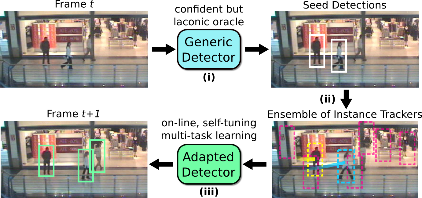
Figure 1: Overview of our approach. (i) A confident but laconic oracle is periodically run along an unseen video stream to generate a few seed detections (candidate bounding boxes with top confidence scores). (ii) The seed objects are tracked along the video with an Ensemble of Instance Trackers (EIT). Our main contribution is that we jointly learn the detectors used by each tracker using an on-line self-tuning multi-task learning algorithm able to leverage difficult samples (in purple). (iii) An adapted model is available anytime from the EIT, and allows to detect objects — beyond just the few seed objects — in the rest of the stream or other videos.

Self-adapting a classifier might suffer from negative transfer, either because of over-fitting to only a few positive samples, or because of drifting due to the inclusion of false positives. Another challenge is that there is in general no way to tune hyper-parameters due to the lack of labeled target validation data. In this work, we address these issues by leveraging the spatio-temporal structure of video data. First, in Section 3, we propose to use multi-task learning in conjunction with tracking as a way to automatically elicit a useful set of target positives and negatives, especially “hard negatives”, which are crucial for high detection performance [2, 3]. Our multi-task learning objective yields an adapted shared latent model of the category, which bridges the gap between instance-level models used for tracking and category-level models used for detection. Second, in Section 4, we detail how to learn this model. We propose a novel efficient on-line algorithm applicable to non-stationary streaming scenarios. Our method rests on the combination of recent stochastic optimization techniques with a novel hyper-parameter self-tuning method exploiting a “no-teleportation and no-cloning” assumption. Experiments, in Section 5, on two challenging real-world datasets illustrate that we are able to learn and adapt detectors from scratch on different scenes with no labeled data.

2 Related work

Unsupervised domain adaptation approaches use annotated data from a fixed dataset (the source set) and only unlabeled data from the target dataset. They often require one or more passes over a large pool of annotated samples in order to adapt the model to each new target dataset, which makes them impractical for continuous adaptation to streaming data. For instance, Taskar et al.  [4] leverage “unseen” features from instances classified with high confidence, learning which features are useful for classification, and Gong et al.  [5] “reshape” datasets to minimize their distribution mismatch. These methods assume that the target domain is stationary, with many unlabeled target samples readily available at each update (transductive setting [6]). Consequently, these approaches are not suited to non-stationary streaming scenarios, such as when using on-board cameras (e.g., for autonomous driving or robotics).

Most related to our work are methods exploiting the spatio-temporal structure of videos in order to collect target data samples. Prest et al.  [7] learn object detectors by relying on joint motion segmentation of a set of videos containing the object of interest moving differently from the background. Their goal is to learn generic detectors that adapt well from video to image data. Tang et al.  [8] are inspired by the self-paced learning approach of Kumar et al.  [1], i.e. “learn easy things first”, which is designed for fine-tuning on target domains related to a labeled source one. The transductive approach of Tang et al.  [8] iteratively re-weights labeled source samples by using the tracks of the closest target samples. Sharma et al.  [9] propose a similarly inspired multiple instance learning algorithm, also relying on self-paced learning and off-line iterative re-training of a generic detector. These approaches can only be applied in stationary transductive settings, and do not allow for efficient model adaptation along a particular video stream.

Several tracking-by-detection methods are also related to our work, in particular the tracking-learning-detection approach of Kalal et al.  [10] and the multi-task learning approach of Zhang et al.  [11]. However, they are designed to work on short sequences, and their goal is to learn only instance-specific models, whereas our aim is to learn and adapt category-level ones. Note that we also differ from the family of multi-class transfer learning methods aiming to share features across categories, such as the “learning to borrow” approach of Lim et al.  [12]. These approaches are different in intent from our continuous category-level adaptation to a new data stream. Furthermore, they are not straightforwardly applicable for object detection with one or few categories of interest (e.g., cars and pedestrians).

3 Multi-task learning of an ensemble of trackers

3.1 Tracking-by-detection

In this work, the term “object detector” denotes a binary classifier parametrized by a (learned) vector ${\bf w}\in\mathbb{R}^{d}$. This classifier computes the probability that a window — an image sub-region ${\bf x}$ represented by a feature vector $\phi({\bf x})\in\mathbb{R}^{d}$ — contains an object of the category of interest by:

$$P({\bf x})=\left(1+e^{-\left({\bf w}^{T}\phi({\bf x})+b\right)}\right)^{-1}.$$ (1)

When a new frame is available, the first step of our method consists in calling a confident but laconic oracle returning a few (or no) automatically labeled samples (image regions with object category labels in our case). We assume that the automatic labels of these seed target samples are mostly correct, which means that they correspond only to the “easiest” target samples (high-precision but low-recall regime). We track each of these seeds in subsequent frames using a simple but efficient tracking-by-detection algorithm inspired by the P-N learning algorithm of Kalal et al.  [10]. The tracker associated to each seed $i$ maintains its own personal detector ${\bf w}_{i}^{(t)}$. This detector is run on a new frame $t+1$ to return a pool of candidate locations. The new location of object $i$ is then simply the candidate region that yields the closest match with the location in the previous frame (after simple motion interpolation based on sparse optical flow). If there is no match, then the object $i$ is considered lost, and it is not tracked further. If a new location is found, then the corresponding region is considered as positive and the other detections as negatives in order to update the model ${\bf w}_{i}^{(t)}$ of object $i$. This relies on both a spatio-temporal smoothness assumption (based on the observed motion of each object instance), and the uniqueness of each object being tracked. In other words, we assume there is neither teleportation, nor cloning of the individual instances.

Note that these negatives are in fact false positives, i.e. “difficult” target samples, also called hard negatives [2]. Contrary to the easier samples used in self-paced learning (e.g., in Tang et al.  [8]), they are key to the successful update of the model. This is, indeed, well established in the object detection community (cf. Felzenszwalb et al.  [3] for instance). Furthermore, we conducted preliminary experiments where directly learning a video-specific detector on seed samples as positives and random negatives consistently resulted in negative transfer (i.e. worse performance than the generic detector oracle alone). We also observed this negative transfer when replacing the automatic seed positives by the ground truth bounding boxes of the moving objects only. Note that our tracking approach does not rely on background subtraction or motion segmentation, and is therefore applicable to stationary objects and moving cameras.

This negative transfer illustrates the difficulty of bridging the gap between instance-level models and category-level ones, and the importance of difficult target samples. Note that there is also a risk of negative transfer when using difficult samples (as they might be wrongly labeled). In the following, we describe how we address these challenges via our novel multi-task tracking formulation to exploit the commonalities between seeds.

3.2 The Ensemble of Instance Trackers (EIT) model

Let $N_{t+1}$ be the number of object instances currently being tracked, each one associated with its own detector ${\bf w}_{i}^{(t)}$. Updating each detector amounts to minimizing the regularized empirical risk:

$${\bf w}_{i}^{(t+1)}=\arg\min_{{\bf w}_{i}}\sum_{k=1}^{n_{i}}\ell({\bf x}_{k}^{(i)},y_{k}^{(i)},{\bf w}_{i})+\lambda\Omega({\bf w}_{i}),\quad i=1,\cdots,N_{t+1}$$ (2)

where ${\bf x}_{k}^{(i)}$ is one of the $n_{i}$ training samples of object $i$ in frame $t+1$ — either a random window (to get negatives during initialization), a seed from the generic detector, or a candidate detection obtained by running the current version of the model ${\bf w}_{i}^{(t)}$ — and $y_{k}^{(i)}$ is a binary label. The labels are obtained using the aforementioned “no teleportation and no cloning” assumption, with the addition that negative samples overlapping any other object currently tracked are not used (a region that is not Ann’s car does not mean it is not a car). Here, $\ell({\bf x},y,{\bf w})$ is the loss incurred by classifying ${\bf x}$ as $y$ using parameters ${\bf w}$, and $\Omega({\bf w})$ is a regularizer. In our experiments, we use the logistic loss:

$$\ell({\bf x},y,{\bf w})=\log\left(1+\exp\left(-y\left({\bf w}^{T}\phi({\bf x})+b\right)\right)\right)\ ,$$ (3)

as this gives calibrated probabilities with Eq. (1), and enjoys useful theoretical properties for on-line optimization [13]. The set of $N_{t+1}$ trackers, with joint detector parameters ${\bf W}^{(t)}=\{{\bf w}_{1}^{(t)},\ldots,{\bf w}_{N_{t+1}}^{(t)}\}$ is denoted as Ensemble of Instance Trackers (EIT). With this notation, we can express the $N_{t+1}$ equations in Eq. (2) as a joint minimization over the ensemble parameters:

$${\bf W}^{(t+1)}=\arg\min_{{\bf W}}L({\bf X}^{(t+1)},{\bf y}^{(t+1)},{\bf W})+\lambda\Omega_{t}({\bf W}),$$ (4)

Clearly, if $L({\bf X}^{(t+1)},{\bf y}^{(t+1)},{\bf W})=\sum_{i}\sum_{k}\ell({\bf x}_{k}^{(i)},y_{k}^{(i)},{\bf w}_{i})$ and $\Omega_{t}({\bf W})=\sum_{i}\Omega({\bf w}_{i})$, we recover exactly Eq. (2) where each classifier is learned independently. In order to jointly learn all the classifiers, we impose the following multi-task regularization term instead:

$$\Omega_{t}({\bf W})=\frac{1}{2N_{t+1}}\sum_{i=1}^{N_{t+1}}\|{\bf w}_{i}-\bar{{\bf w}}^{(t)}\|_{2}^{2}.$$ (5)

where $\|{\bf w}_{i}\|_{2}$ denotes the $l_{2}$ norm of ${\bf w}_{i}$, and $\bar{{\bf w}}^{(t)}$ is the (running) mean of all previous instance models, which comprises all past values of the models of currently tracked or now lost seed-specific detectors. Note that this formulation is closely related to the mean-regularized multi-task learning formulation of Evgeniou and Pontil [14], with the difference that it is designed for on-line learning in streaming scenarios. This regularization promotes solutions where classifiers (past and present) are similar to each other (in the Euclidean sense). Therefore, this regularization prevents each detector from over-fitting to the appearance of the individual object appearances, and allows them to generalize across tasks (object instances) by modeling the latent commonalities (the appearance of the category) with the mean of the trackers.

Importantly, this provides a theoretical justification to using the running average $\bar{{\bf w}}^{(t)}$ as a single category-level detector. Consequently, once the detectors ${\bf w}_{i}$ are updated in frame $t+1$, a new scene-adapted detector is readily available as:

$$\bar{{\bf w}}^{(t+1)}=\frac{1}{\bar{N}_{t}+N_{t+1}}\left(\bar{N}_{t}\bar{{\bf w}}^{(t)}+\sum_{i=1}^{N_{t+1}}{\bf w}_{i}^{(t+1)}\right)\ ,$$ (6)

where $\bar{N}_{t}=\sum_{\tau=1}^{t}N_{\tau}$. In our object detection case, this approach can be interpreted as learning a category-level model from the average of instance-specialized models. As we use linear classifiers, this multi-task learning could be seen as an improvement of “late fusion” of exemplar-based models, such as the Exemplar-SVM of Malisiewicz et al.  [15]. A major difference is that our models are learned jointly and adapt continuously to both the data stream and other exemplars.

Another benefit of this regularization is that it learns a model that is more robust to erroneous seeds (initial false detections of the generic detector), as they are likely to significantly differ from the mean, and, therefore, the corresponding trackers will be quickly under-fitting and lose the object. In contrast, the correct seeds will be tracked for longer, as they share common appearance factors, thus contributing more to the category model. Note, however, that the $l_{2}$-norm used in Eq. (5) is not robust to outliers. Therefore, the handling of incorrect seeds could be improved by using more robust alternatives — e.g., sparsity-inducing or trace-norm regularizers, replacing the mean by the median, or outlier detection methods — at the cost of a more computationally demanding solution, which is also more complex to update on-line than our running average. Our approach is compatible with these improved regularizers, but we focus on the simple regularization of Eq. (5) in order to directly show the potential of our self-tuning on-line multi-task learning algorithm described next.

4 Continuous self-tuning on-line adaptation

4.1 Streaming asynchronous optimization

We solve the optimization problem in Eq. (4) using Averaged Stochastic Gradient Descent (ASGD), also called Polyak-Rupert averaging [16]. This on-line first order method achieves optimal convergence rate with only one pass over the data and a constant learning rate with a logistic regression model [13]. The update rule for each model ${\bf w}_{i}$ is:

$${\bf w}_{i}^{(t+1,k)}={\bf w}_{i}^{(t+1,k-1)}-\eta\left(\frac{\partial\ell}{\partial{\bf w}}({\bf x}_{k}^{(i)},y_{k}^{(i)},{\bf w}_{i}^{(t+1,k-1)})+\frac{\lambda}{N_{t+1}}\left({\bf w}_{i}-\bar{{\bf w}}^{(t)}\right)\right),$$ (7)

where $\eta$ is the learning rate, $({\bf x}_{k}^{(i)},y_{k}^{(i)})$ a training sample, $k=1,\cdots,n_{i}$, and ${\bf w}_{i}^{(t+1,0)}={\bf w}_{i}^{(t)}$. The actual model used is then the average of all previous updates, which is simply obtained by maintaining a running mean of the updates to compute:

$${\bf w}_{i}^{(t+1)}=\frac{1}{n_{i}}\sum_{k=1}^{n_{i}}{\bf w}_{i}^{(t+1,k)}$$ (8)

Equations (4),(5), (6) and (7) show that the learning process is a joint one: the update of the detector ${\bf w}_{i}$ includes a contribution of all the other detectors (both current and past ones). Another advantage is that our approach is well suited to a streaming and asynchronous scenario, as the update of each specific model ${\bf w}_{i}$ only relies on the current frame and the current running average of all models. In practice, we use a mini-batch variant of ASGD with potentially multiple passes over the data available at time $t+1$. This allows to share window preprocessing operations at the frame level, and reduces the variance of the gradients. We also maintain the running average of the parameters not only across gradient descent steps, but also across frames (not depicted in Eq. (8) for simplicity).

4.2 Self-tuning of hyper-parameters

A key issue in our unsupervised on-line learning setting is how to select the values of the different hyper-parameters involved, amongst which are the learning rate $\eta$ in Eq. (7), the regularization parameter $\lambda$ in Eq. (4), and the number of iterations per mini-batch. This is particularly important, as we have to continuously update appearance models in a streaming fashion, where data samples are likely to be non-i.i.d. , and the video stream to be non-stationary (e.g., in long-term surveillance scenarios). The learning rate, in particular, is a crucial parameter of ASGD, and should be set on a per-update basis in this non-stationary case.

Cross-validation, typically used to tune hyper-parameters, is not applicable in our setting, as we have only one positive example at a time. Furthermore, optimizing the window classification performance is not guaranteed to result in optimal detection performance due to the additional post-processing steps applied in most detection methods [17].

Instead, we use a strategy consisting in greedily searching for the least-over-fitting parameters — e.g., smallest $\eta$ and number of iterations, largest $\lambda$ — that optimize the rank of the correct detection in the current frame. This only involves running the detector after each tentative update in order to assess whether it yields a top ranked detection strongly overlapping with the tracker’s prediction, and is efficient in practice, as it re-uses the already extracted frame-level computations (in particular the feature extraction). See Figure 2 for a high-level pseudo-code description of our method.

(a) Self-learning camera algorithm

1:  Input: generic detector, video stream

2:  Output: adapted detector $\bar{{\bf w}}^{(t+1)}$

3:  Initialization: $\bar{{\bf w}}^{(0)}=\mathbf{0}$, $\mathcal{W}=\emptyset$

4:  while video stream is not finished do

5:     Get seeds not in $\mathcal{W}$ from the generic detector on current frame $t+1$

6:     for each new seed do

7:        Learn initial detector warm-started from $\bar{{\bf w}}^{(t)}$ with random negatives

8:        Add to pool of instances $\mathcal{W}$

9:     end for

10:     for each instance $i$ in $\mathcal{W}$ do

11:        Run the detector ${\bf w}_{i}^{(t)}$

12:        if object $i$ is lost then

13:           Remove $i$ from $\mathcal{W}$

14:        else

15:           Get $\{({\bf x}_{k}^{(i)},y_{k}^{(i)}),\ k=1:n_{i}\}$ from the detections (cf. Sec. 3)

16:           Compute ${\bf w}_{i}^{(t+1)}$ (cf. Alg. 2(b))

17:        end if

18:     end for

19:     Compute $\bar{{\bf w}}^{(t+1)}$ (Eq. 6)

20:  end while

(b) Autonomous self-tuning adaptation

1:  Input: ${\bf w}_{i}^{(t)}$, $\{({\bf x}_{k}^{(i)},y_{k}^{(i)}),\ k=1:n_{i}\}$ with ${\bf x}_{p}^{(i)}$ the current location estimate of $i$

2:  Output: ${\bf w}_{i}^{(t+1)}$

3:  for $n_{\text{steps}}\in\{1,10,100\}$ do

4:     for $\lambda\in\{1.0,0.9,0.5,0.1\}$ do

5:        for $\eta\in\{10^{-5},10^{-4},\cdots,10^{-1}\}$ do

6:           Compute tentative ${\bf w}_{i}^{(t+1)}$ (Eq. 8)

7:           Run detector ${\bf w}_{i}^{(t+1)}$

8:           Compute rank of detection matching ${\bf x}_{p}^{(i)}$ (if any)

9:           if rank is $1$ then

10:              return  ${\bf w}_{i}^{(t+1)}$

11:           end if

12:        end for

13:     end for

14:  end for # In case no update yielded rank $1$

15:  return  ${\bf w}_{i}^{(t+1)}$ with best ranked prediction

Figure 2: Pseudo-code overview of our approach (book-keeping operations like maintaining counters and running averages are not described for simplicity, refer to the main text for more details)

5 Experiments

5.1 Datasets

In order to validate our approach, we use publicly available benchmarks: five video sequences from CAVIAR, and a long HD video sequence from VIRAT. Objects of interest in CAVIAR are persons, while VIRAT objects of interest are cars. Sample images from the two scenarios are shown in Figure 3. Some dataset details are reported in Table 1.

On CAVIAR, we use the same sequences as Wang et al.  [18] — Ols1, Ols2, Osow1, Olsr2, and Ose — and also upscale the image size by a factor of 2.0. We run independent experiments on each of the five sequences. Each sequence is used both for unsupervised learning and evaluation (i.e. the same setting as in [18]). In our case, this corresponds to a scenario where the object detector is continuously adapted along a finite video stream, to later be applied to the entirety of this video. Note that we compare to Wang et al.  [18], a state-of-the-art unsupervised video adaptation method also relying only on a pre-trained generic detector, and assuming the most confident detections are true positives. In contrast to our approach however, Wang et al.  [18] propose a “lazy learning” method consisting in re-ranking the low scoring detections using the similarity to high scoring ones. While this re-ranking process improves the detection performance, the method does not produce an adapted detector, and can, therefore, only be applied in a batch setting, as on the CAVIAR dataset.

For VIRAT, we use sequence 0401, because it is fully annotated with both static and moving objects, and corresponds to a typical parking scene. The size (375K objects) and duration of VIRAT-0401 (58K frames) allows splitting the sequence in two parts (of equal length). Our self-learning algorithm is run on the first part of the video to self-learn and autonomously adapt the specific detector, whose generalization performance (on different scenes from the same target domain) is then evaluated on the second part of the video stream.

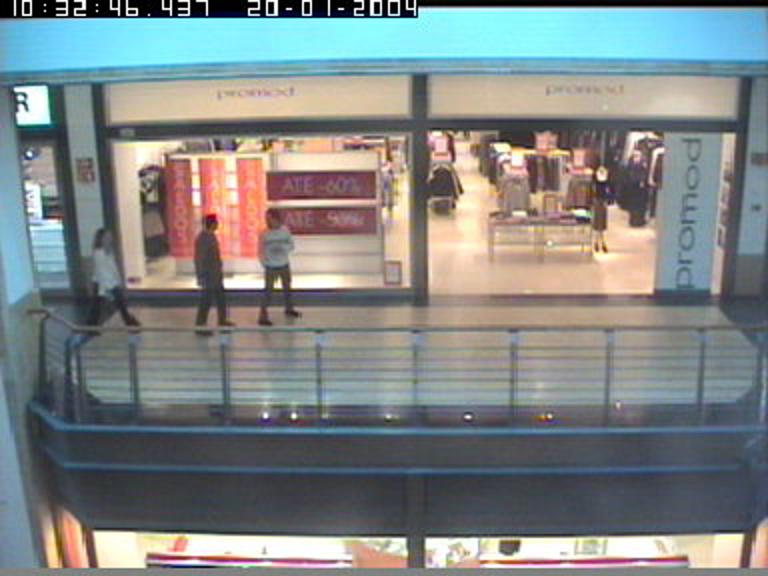
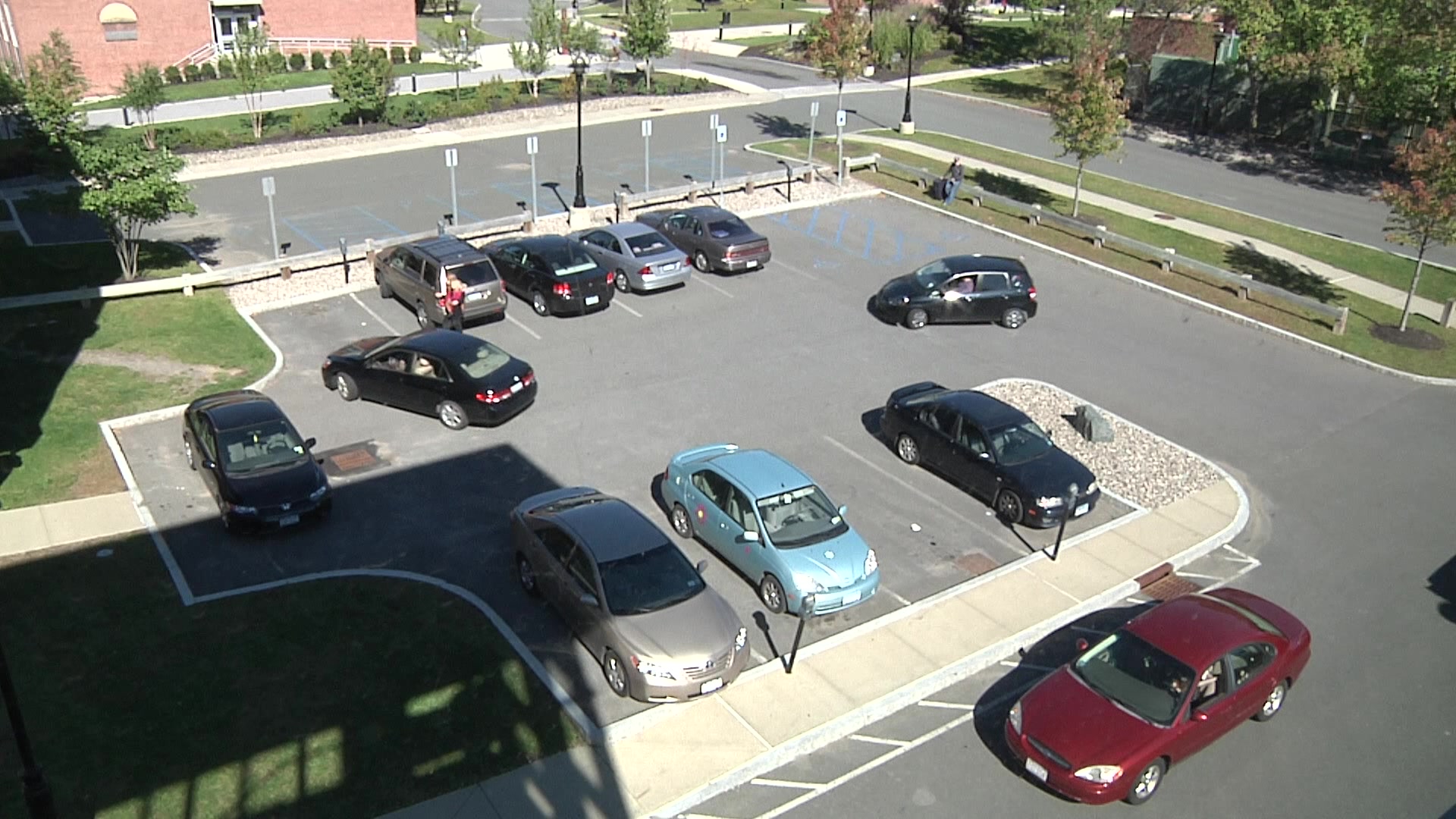
Figure 3: Frames from the CAVIAR (left) and VIRAT-0401 (right) datasets.

	frame size	fps	#frames	class	#objects
CAVIAR (Ols1)	576 $\times$ 768	25	295	pedestrian	438
CAVIAR (Ols2)	576 $\times$ 768	25	1119	pedestrian	290
CAVIAR (Osow1)	576 $\times$ 768	25	1377	pedestrian	2402
CAVIAR (Olsr2)	576 $\times$ 768	25	560	pedestrian	811
CAVIAR (Ose2)	576 $\times$ 768	25	2725	pedestrian	1737
VIRAT-0401	1080 $\times$ 1920	30	58$K$	car	375$K$

Table 1: Video object detection datasets used in our experiments

5.2 Implementation details

Generic detector oracle

Like in [18], we use the state-of-the-art Deformable Part Model (DPM) [3] as our black box generic object detector. This generic detector is pre-trained on Pascal VOC 2007, and is publicly available online. The performance obtained by DPM is reported in Table 2. In order to use DPM as a confident but laconic oracle, we use only its top $5\%$ detections.

Tracking-by-detection object detector

Our formulation is applicable to any detector based on a linear classifier, and is, therefore, usable with most state-of-the-art object detection and window representation methods [3, 17, 19]. In our experiments, we use Fisher Vectors (FV) [20], as this representation is particularly suited to our problem for the following reasons. First, FV are among state-of-the-art representations for object detection [17]. Second, they proved to be efficient for both category-level image classification [21] and instance-level retrieval problems [22]. This highlights their potential for both category-level and instance-level appearance modeling. Third, FV are high-dimensional representations, which allows our mean-regularized multi-task learning to, in principle, be able to model complex distributions using a single linear representation. To the best of our knowledge, our method is the first application of FV to tracking.

In our experiments, we followed the implementation of Cinbis et al.  [17], which yields competitive detection results on Pascal VOC, with the difference that we use a more efficient but approximate sliding window approach similar to the one described in Oneata et al.  [23].

5.3 Results

	Ols1	Ols2	Olsr2	Osow1	Ose2	VIRAT-0401
DPM [3]	30.4	52.4	34.9	52.2	34.8	47.0
DbD [18]	32.1	56.3	43.1	47.0	40.9	N.A.
I-EIT	27.4	53.6	40.6	51.9	38.9	53.1
EIT	29.3	58.0	43.7	53.1	38.1	53.7

Table 2: Detection performance (Average Precision). “DPM” is the pre-trained generic detector (DPM [3], using all detections, not just seeds). “DbD” is the re-ranking of the “DPM” detections using the algorithm of Wang et al.  [18]. “I-EIT” is a baseline adapted detector from our Ensemble of Instance Trackers without multi-task penalization, i.e. with independent trackers. “EIT” is the adapted detector obtained with our “self-learning camera” multi-task learning algorithm.

Table 2 contains our quantitative experimental results. Performance is measured using Average Precision (AP), which corresponds to the area under the precision-recall curve. It is the standard metric used to measure object detection performance [24]. Our results using the adapted detector obtained by our multi-task Ensemble of Instance Trackers are reported in the “EIT” row.

We compare our approach to three other object detectors applicable in our unsupervised setting: (i) the pre-trained DPM detector used alone over the whole video; (ii) our implementation of the “Detection by Detections” (DbD) unsupervised object detection approach of Wang et al.  [18]; (iii) our EIT algorithm without multi-task regularization, i.e. where the trackers are learned independently, which is referred to as “I-EIT”. Note that we do not compare to additional unsupervised video adaptation methods (e.g.,  [8, 9]), as our contribution is on autonomous on-line self-adaptation, i.e. we do not assume access to a large fixed labeled dataset related to the target videos, or that all target video frames are available at once (in contrast to [8, 9]).

First, we can observe that our approach improves over the generic detector by $+4\%$ on average over the scenarios. This confirms that unsupervised learning from scratch of our simple and efficient detector for a specific video stream can outperform a state of the art, carefully tuned, complex, and generic object detector trained on large amounts of unrelated data. Note that we improve in all scenarios but one (Ols1), which corresponds to the smallest video, which is of roughly ten seconds (cf. Table 1). This means that this video is not enough to learn a detector that is better than the generic detector trained on much more data (thousands of images in the case of Pascal VOC).

Second, jointly learning all trackers (EIT) improves by $+1.7\%$ on average over learning them independently. For some scenarios, the gain is substantial ($+4.4\%$ on Ols2), while for one scenario it slightly degrades performance ($-0.8\%$ on Ose2). On the one hand, this illustrates that our multi-task tracking formulation can help learning a better detector when the tracked seed instances share appearance traits useful to recognize the category of objects of interest. On the other hand, this calls for a more robust multi-task learning algorithm than our simple mean-regularized formulation in order to handle more robustly outliers and the large intra-class variations typically present in broad object categories like cars.

Third, our approach yields a small improvement over the state-of-the-art DbD method ($+0.6\%$ on average over the CAVIAR scenarios). This suggests that our approach is accurate enough to discard the generic detector after seeing a large enough part of the video stream (to get enough seeds), whereas DbD must constantly run the generic detector, as it is a “lazy learning” approach based on $k$-nearest neighbors (it does not learn a stand-alone detector). Note also that DbD could be applied as a post-processing step on the results of our detector in order to improve performance, but this leads to additional computational costs.

References

- [1] P. Kumar, B. Packer, and D. Koller, “Self-paced learning for latent variable models,” in NIPS, 2010.
- [2] N. Dalal and B. Triggs, “Histograms of oriented gradients for human detection,” in CVPR, 2005.
- [3] P. Felzenszwalb, R. Girshick, and D. McAllester, Dand Ramanan, “Object detection with discriminatively trained part-based models,” PAMI, 2010.
- [4] B. Taskar, M.-F.Wong, and D. Koller, “Learning on the test data: Leveraging ‘unseen’ features,” in ICML, 2003.
- [5] B. Gong, K. Grauman, and F. Sha, “Reshaping visual datasets for domain adaptation,” in NIPS, 2013.
- [6] T. Joachims, “Transductive inference for text classification using support vector machines,” in ICML, 1999.
- [7] A. Prest, C. Leistner, J. Civera, C. Schmid, and V. Ferrari, “Learning object class detectors from weakly annotated video.,” in CVPR, 2012.
- [8] K. Tang, V. Ramanathan, L. Fei-Fei, and D. Koller, “Shifting weights: Adapting object detectors from image to video,” in NIPS, 2012.
- [9] P. Sharma, C. Huang, and R. Nevatia, “Unsupervised incremental learning for improved object detection in a video,” in CVPR, 2012.
- [10] Z. Kalal, K. Mikolajczyk, and J. Matas, “Tracking-learning-detection,” PAMI, 2012.
- [11] T. Zhang, B. Ghanem, S. Liu, and N. Ahuja, “Robust visual tracking via structured multi-task sparse learning,” IJCV, 2013.
- [12] J. J. Lim, R. Salakhutdinov, and A. Torralba, “Transfer learning by borrowing examples for multiclass object detection,” in NIPS, 2011.
- [13] F. Bach and E. Moulines, “Non-strongly-convex smooth stochastic approximation with convergence rate O ( 1 / n ),” in NIPS, 2013.
- [14] T. Evgeniou and M. Pontil, “Regularized multi–task learning,” in SIGKDD, 2004.
- [15] T. Malisiewicz, A. Gupta, and A. Efros, “Ensemble of Exemplar-SVMs for object detection and beyond,” in ICCV, 2011.
- [16] B. Polyak and A. Juditsky, “Acceleration of stochastic approximation by averaging,” SIAM Journal on Control and Optimization, 1992.
- [17] R. Cinbis, J. Verbeek, and C. Schmid, “Segmentation driven object detection with Fisher vectors,” in ICCV, 2013.
- [18] X. Wang, G. Hua, and T. Han, “Detection by detections: Non-parametric detector adaptation for a video.,” in CVPR, 2012.
- [19] R. Girshick, J. Donahue, T. Darrell, and J. Malik, “Rich feature hierarchies for accurate object detection and semantic segmentation,” in CVPR, 2014.
- [20] F. Perronnin and C. Dance, “Fisher kernels on visual vocabularies for image categorization,” in CVPR, 2007.
- [21] J. Sánchez, F. Perronnin, T. Mensink, and J. Verbeek, “Image Classification with the Fisher Vector: Theory and Practice,” IJCV, 2013.
- [22] H. Jégou, F. Perronnin, M. Douze, J. Sánchez, P. Pérez, and C. Schmid, “Aggregating local image descriptors into compact codes,” PAMI, 2012.
- [23] D. Oneata, J. Verbeek, and C. Schmid, “Efficient Action Localization with Approximately Normalized Fisher Vectors,” in CVPR, 2014.
- [24] M. Everingham, L. Van Gool, C. Williams, J. Winn, and A. Zisserman, “The pascal visual object classes (voc) challenge,” IJCV, 2010.