section
Topology of the Misner Space
and its -boundary
Juan Margalef–Bentabol1,2 Eduardo J. S. Villaseñor2 juanmargalef@ucm.es ejsanche@math.uc3m.es
1 Instituto de Estructura de la Materia, CSIC, Serrano 123, 28006 Madrid, Spain. 2 Unidad Asociada al IEM-CSIC, Grupo de Teorías de Campos y Física Estadística, Instituto Universitario Gregorio Millán Barbany, Grupo de Modelización y Simulación Numérica, Universidad Carlos III de Madrid, Madrid, Spain
Abstract
The Misner space is a simplified 2-dimensional model of the 4-dimensional Taub-NUT space that reproduces some of its pathological behaviours. In this paper we provide an explicit base of the topology of the complete Misner space . Besides we prove that some parts of this space, that behave like topological boundaries, are equivalent to the -boundaries of the Misner space.
1 Introduction
The Taub-NUT space-time is a spatially homogenous vacuum solution to the Einstein equations that displays many strange behaviours. In order to understand some of its pathologies C.W. Misner introduced in a seminar entitled Taub-NUT space as a counterexample to almost anything [14], a simpler -dimensional model, the so-called Misner space. This space-time has still some strange behaviours that have been carefully studied in [8, 17], and besides, it has been used as a toy-model for different purposes like big bounce models [1, 9].
The geometrical and topological properties of Misner space can be derived by constructing it in terms of the quotient space . Following this approach, we do not only recover the Misner space but also prove that some subsets of it behave like the -boundaries introduced by S.W. Hawking [7] and R. Geroch [3]. It is important to point out that the abstract definition of the -boundary of a semiriemannian manifold is highly non trivial and, in practice, it is very difficult to compute it from the definition. In fact, in [3] and [6] some examples are obtained but no computation is provided. This construction has an even worse problem: whenever a boundary construction verifies, as the -boundary does, some reasonable conditions, then a space-time can be constructed with unphysical boundary [5]. Even the fact of being defined using geodesics is not satisfactory owing to an example due to R. Geroch [4] of a geodesically complete space-time containing curves of finite length and bounded acceleration (hence there exist physical time-like observers that are incomplete). In part due to these problems, the study of this and similar constructions has been essentially abandoned. We think, however, that it is still interesting to verify that in the case of the complete Misner space, the -boundary is what one expects to be. Besides, for some of these completions, such as for the -boundary, there exists a canonical way of defining a minimal refining of the topology such that the points of the boundary become T2-separated from all the rest of the points [2] removing some of the worst problems of these constructions; hence, they may regain some interest in the recent future.
The paper is structured as follows, in section 2 we carefully study the Misner space as a quotient space, providing an explicit base of the quotient topology and deducing from it some topological properties (and problems). In section 3 we discuss, in some detail, the behaviour of the light-like geodesics in the extended Misner space. The concept of the -boundary is introduced in section 4 and apply it to the the Misner space. We show that the topology defined by the -boundary coincides, precisely, with the quotient topology obtained in section 2. We end this paper in section 5 with the discussion of the main results and our conclusions. For the convenience of the reader, we also provide an appendix where the necessary mathematical background is presented.
2 The Misner space as a quotient space
In this section, we construct the Misner space by considering the quotient space of the Minkowski space-time under a discrete group of Lorentz boosts. In this approach, arises as the quotient space (or, equivalently ), which will allow us to understand the pathological behaviour of its geodesics. Moreover, by considering the quotient over two adjacent quadrants of plus the line in between them (e.g ), we get an isometric extension of , that we will refer to as the extended Misner space. This extension partially solves the geodesic incompleteness problem of . However, as we will see, it is not possible to extend further to completely solve the the geodesic incompleteness.
2.1 General facts about the Misner space
The Lorentz group is formed by the linear maps , which preserve the Minkowski product . The subgroup composed by the space-orientation preserving and the time-orientation preserving maps is called special orthochronous Lorentz group:
where is the velocity of one inertial frame with respect to another one, can be interpreted as the rapidity [12] and, as usual, . The boosts matrices satisfy the following:
Properties.
-
P.1
As is linear, it maps lines (through the origin) to lines (through the origin),
![[Uncaptioned image]](/html/1406.4552/assets/x1.png)
and it has as invariant lines the diagonals . Indeed each semi-line is invariant. P.2 where for a fixed given quadrant , we denote the open semi-line in that begins at the origin with hyperbolic angle . From now on, is the corresponding open quadrant (in between the diagonals) and is the corresponding open semi-diagonal where the origin is excluded. P.3 where is the line with slope that cuts the semi-diagonal at the point . P.4 For , the sets are invariant. Notice that for , the hyperbolas are space-like and are time-like.
![[Uncaptioned image]](/html/1406.4552/assets/x2.png)
If then is an infinite cyclic group, and for every , the orbit is an infinite countable set. This action over is properly discontinuous and free. In particular, if , then:
Thus, for forward iterations, the points over the diagonal accumulate over the origin exponentially while the points over the diagonal grow to infinity exponentially. By using the exponential map , , it is clear that each of the quotient spaces is homeomorphic to a circle .
The action of over is also properly discontinuous and free. In particular (resp. ) is a smooth Hausdorff manifold homeomorphic to the cone (resp. ). In fact, by expressing the Minkowski metric in hyperbolic coordinates the action of is given by and the metric in is:
In particular, the circles are space-like. Notice that for , both are isometric to the Misner space:
The future directed light-like geodesics over the Misner space are:
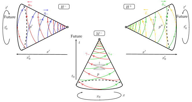
where we have replaced by in order to emphasize that ranges over . The geodesics satisfy , , and . Summarizing, we have that the two future directed light-like geodesics obtained are incomplete as , but notice that, as is increasing and grows to infinite, they turn around the cylinder infinitely many times. We can see graphically the behaviour of the geodesics in figure 1, the closer to (which corresponds to the apex, and hence it does not belong to ), the quicker with respect to the affine parameter a light-like geodesic turns around the cylinder.
Similarly, (resp. ) is a smooth Hausdorff manifold homeomorphic to the cone . In hyperbolic coordinates , the metric in is
In this case, the circles are time-like. The future directed light-like geodesics over are:
Notice that now is the periodic coordinate and we have , and . The light-like geodesics of would have the same expressions (we could replace by ) with aiming also towards the apex.
If we now consider the quotient over the whole plane, , we do not obtain a smooth manifold as the origin is a fixed point, furthermore some other problems arise as we will see in section 2.4. However the action over one of the semi-planes is free and properly discontinuous, so the quotient is a smooth Hausdorff manifold which topologically is homeomorphic to two cones without the apex (one for each quadrant) and a circle corresponding to the semi-diagonal. The cones can be deformed into semi-cylinders and glued along the circle to obtain a whole cylinder. In particular, the metric in the extended Misner space can be written as:
where the coordinates are related to those on and through
Notice that the light-like circle corresponds to . On the other hand, the metric in the extended Misner space is:
where
In this case the light-like circle corresponds to .
From now on, let us focus on . The light-like geodesics can be expressed in the - coordinates to give the future directed () light-like geodesics of passing through :
Similarly, the future directed light-like geodesics of passing through are:
where notice that now . Clearly and can be extended to , in fact, they can be glued together through its limit point at the level. However the geodesics and cannot be extended and remain incomplete. Notice that for all the geodesics.
We see that we have partially solved our “pathology” as we have managed to “unwrap” and , but we have “wrapped twice” and . The case has to be studied separately:
Remark 2.1.
The future directed light-like geodesics with are
is exactly the complete and glued through their limit point, while is incomplete, remains always in the subset and verifies (as well as and ). Furthermore it verifies a quite astonishing property. For a given if we define a for every such that:
then we have that for every :
Hence the curve passes infinitely many times through the same point but with “longer” tangent vector (but notice that its modulus remains constant and equal to zero!).
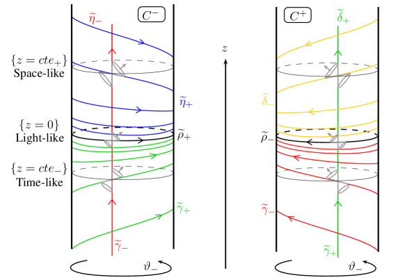
For the extended coordinates we have analogous results, although now the roles of each pair of geodesics are exchanged, and of course, we have to consider and instead of and (see figure 2). Besides, this construction can be used to obtain an incomplete compact spacetime [10, page 77] by gluing a positive slice and a negative one with a suitable deformation, obtaining a torus with the slice in it.
We see then that we have two inequivalent inextensible extensions of , however they both turn out to be again incomplete. Once at that point we should try to understand why this happens and if it is possible to find an even better coordinate system to solve the pathology completely. Notice that in order to extend the space-time , we have followed the incomplete geodesics and we have defined a new coordinate to extend them, so one might wonder if we can do the same over the extensions and find where the wrapped geodesics go. It is not hard to believe that they go to the upper cone (isometric to the lower one under the mapping , see figure in section 3) but if we apply the same technique to solve the double wrapped geodesics, we will find that the already “straight” ones, become wrapped again. Actually, as we mentioned before, no further extension exists and here is where topology will turn out to be essential to understand why the pathological behaviour appears in the first place and why we can partially, but not completely, get rid off it.
2.2 Topology induced by the discrete hyperbolic rotation
We will now provide a local base for the topology of the complete Misner space . To this end we are going to consider some local base of and saturate their open sets to obtain a base of the quotient topology (see ‣ A.13).
-
In local hyperbolic coordinates can be written as . Let us define
Using -, we have
In order to saturate, we have to join all these possible images (see remark A.12):
Finally we consider the local base for every with small enough such that does not contain two related points (hence the union is disjoint). If we now look at the glued space, we have simply an open “squared” ball over the cone.
![[Uncaptioned image]](/html/1406.4552/assets/x5.png)
-
Let (analogously for the remaining just changing some signs), we define
Using - we have and then
Finally we take the local base with small enough such that does not contain the origin and does not contain two related points.
As the ball is a bunch of (finite piece of) light-like geodesics each one having a piece over , a piece over , and a point over the diagonal , hence over the glued space we have a bunch of geodesics each having a piece over , a piece over and a point over . Therefore given a point , any basic open neighbourhood over the glued space is an open interval over , together with two “thickened” geodesics (similar to ), each one turning infinitely many times around the corresponding adjacent cone, where the direction of rotation is determined by the evolution of the geodesics over the universal cover as we explain in section 3.
![[Uncaptioned image]](/html/1406.4552/assets/x6.png)
-
We define
Using again - we obtain:
Saturating it, we obtain the region in between the four branches of the hyperbolas and (pushing the lines to infinity):
Each branch of the hyperbola correspond to a “straight” circle over each cone ( in the Misner space). Taking all the hyperbolas with gives simply an annulus around the apex on each cone. The case correspond to the diagonals, which in the glued space are the four circles plus the conic center. Hence a basic open neighbourhood of the origin is the point itself, the four circles and four annulus of “length” on each cone.
![[Uncaptioned image]](/html/1406.4552/assets/x7.png)
2.3 Topological properties of the extended quotient
As every point has a countable base, the space is a first-countable space, indeed we can consider just the points with rational coordinates and we obtain that the space is in fact second-countable. When we restrict the action to one of the semi-planes we obtain a smooth Hausdorff manifold, but whenever we extend the action including two adjacent semi-diagonals, we have that it is no longer Hausdorff, as can be seen taking (saturated) basic open sets and with and . If we consider two points of the same diagonal without the origin, we can choose small enough neighbourhoods such that they do not overlap.
![[Uncaptioned image]](/html/1406.4552/assets/x8.png)
Moreover, as we see on the last image of the previous section, the origin cannot be separated from any point of the circles as they are contained in any open neighbourhood of the origin. Let us then study which separation axioms does the quotient spaces verify (see section A.1):
Proposition 2.2.
-
1.
The quotient space is T0 but not T1.
-
2.
The quotient space is T1 but not T2.
-
3.
The quotient spaces are T2.
-
4.
Every (analogously of ) is not closed over but it is closed over .
Proof.
The only tricky statement is the last one. First notice that removing the origin we have a T1 space, so we might expect that the origin fails to be closed, but surprisingly it is closed. However for every we have that is not open. If we regard the universal cover, we see that the problem lies on the fact that the equivalence class of is a countable set that accumulates over the origin but that does not contain it, so is not closed in (but it is closed in , where it has no accumulation point). On the other hand, the equivalence class of the origin is just a point which is closed over the plane (this is a general result for quotient topologies).
2.4 Problems with the extension of the group action
The statements made in the preceding sections allow us to know why the action group does not work nicely over some regions (see definition \sectionrefdefinition properly discont.2 on appendix B). The action over the whole plane without the origin is free and verifies , but it fails to satisfy . Here we see perfectly why the apparently weird property is required in order to ensure that the resultant manifold is Hausdorff. If we consider the action over the whole plane, we will not obtain a smooth manifold as the origin is a fixed point of , in fact the action is neither free nor , and hence we will obtain a non-smooth non-Hausdorff manifold (known as non-Hausdorff orbifold).
Remark 2.3.
The continuation over of any geodesic of going through the origin, is not univocally determined as it can be broken at the origin. In fact two different geodesics in may merge into one over . Despite this pathology, we have a natural way of assigning the continuation, namely, following the straight line over the universal cover.
3 Further Considerations about the whole Misner Space
Some behaviours of the Misner space can be illustrated in the following figure (compare with fig. 2).
![[Uncaptioned image]](/html/1406.4552/assets/x9.png)
In this figure we see, for instance, why the character of the coordinates is exchanged depending on the sign of the -coordinate in the extended Misner space . It is also important to notice that the spinning happens in the specific sense it does depending on the direction of the corresponding geodesic over the universal cover.
Summarizing, if we reach the apex turning infinitely many times, we will “jump” to the adjacent circle (the right one for the clockwise and the left one for the counterclockwise with respect to the origin), touch it at exactly one point and “jump” again to the next quadrant, according to the rules described by the arrows shown in the previous figure. The other possibility is reaching the apex without turning infinitely many times, which means that over the universal cover we have not crossed any semi-diagonal, hence the geodesic crosses through the origin. The time-like geodesics through the origin must go from to . Over the glued space they are world lines that reach the apex of without turning infinitely many times, “jump” to the origin and “jump” again to . The light-like geodesics through the origin are precisely the semi-diagonals . Over the glued space these geodesics turn on one of the lower circles or infinitely many times but with a finite affine parameter, then “jump” to the origin and finally “jump” again to the opposite circle as the arrows of the figure suggest. The quotations in the word jump come from the fact that according to the topology, no jump exists (such curves are of the form , a composition of continuous functions -see def. A.7-).
It is worth mentioning that quite often this space is not depicted completely right [1, 9, 11] as the circles are missing. Probably this lack of precision is not important for many purposes, but it is of capital importance if we want to understand in detail the Misner space.
Remark 3.1.
A uniformly accelerated observer over the lateral quadrants or follows a hyperbola (through translation we may consider that it has the semi-diagonals as its asymptotes). As this kind of hyperbolas over those quadrants are the time-like circles over the lateral cones, those observers describe closed time-like curves over the glued space.
![[Uncaptioned image]](/html/1406.4552/assets/x10.png)
Any inertial observer over the lateral cones will eventually jump to the upper cone in the same way that any observer in the Minkowski space-time that does not pass through the origin will eventually reach the semi-diagonals , hence the only way that an observer can remain on the lateral cylinders is by experiencing a perpetual acceleration. Besides notice that all the time-like geodesics that do not cross the origin will be tangent to some hyperbola over the lateral quadrants (the slope of these hyperbolas tend to ). Computing the intersection between the geodesic and a generic hyperbola , and imposing the tangency condition, gives that the maximum hyperbolic radius (and hence the “lateral height”) attained in the lateral cones is:
Over the upper and lower quadrants, it crosses every possible hyperbola and hence over the cones it goes from and goes to (where the coordinate is defined separately over each cone). It is interesting also to describe what would happen over the extended space : the time-like geodesic will turn finitely many times around the lower semi-cylinder, cross the level set, turn finitely many times until the maximum of the coordinate is reached. From this point on, the geodesic falls again towards but now turning infinitely many times. Notice in particular that the geodesic is incomplete as is formed gluing and through the circle , but not the upper cone .
4 -boundary
The results presented in the previous sections show that some parts of the extended Misner space, namely the circles and the origin, behave somehow like boundaries of the “adjacent cones” in the sense that every incomplete geodesic of the cones has a limit point that is over the circles or in the origin. The behaviour of these sets resembles that of the -boundary introduced by Hawking [7] and Geroch [3]. Therefore it is worth to compute the -boundary of and see if, as expected, we recover the two adjacent circles and the origin obtained with the quotient topology.
The construction of the -boundary provides a way to build, and glue properly, a boundary to an incomplete semiriemannian manifold . The idea is quite tricky as this completion has to be done just making reference to the manifold itself to define something that will be “outside” of it. It is important to notice that the same manifold space can have different -boundaries (end-points of the incomplete geodesics regarded in the ambient space) depending on the metric. For instance consider the unitary disk :
-
If we use the Euclidean metric, all the geodesics are incomplete and the boundary is .
-
If we consider it to be the Poincaré’s disk with the hyperbolic metric, then all the geodesics are complete and hence the boundary is empty.
-
If we consider the topological disk as the whole sphere without the north pole with the round metric, we see that the boundary is just a point. Now and the round metric can be pulled-back to the unitary disk through the stereographic projection followed by a contraction . Hence, with this particular metric, is just one point.
Now we proceed with a quick review of Geroch’s method to build the -boundary.
4.1 Short review of the construction of the -boundary
Let be a semiriemannian manifold and . For any there exists a unique maximal geodesic such that and . By geodesic we understand a standard geodesic (not just pregeodesic) defined over with . With this notation, the complete geodesics are the “forward complete” geodesics. The reason for doing this is that we can then bijectively associate the geodesics with the reduced tangent bundle . We now define the function:
such that is the total affine length (in the forward direction) of the corresponding geodesic . Clearly is infinite if and only if the geodesic in question is complete. We now define the sets:
is formed by the incomplete geodesics, is the set of all possible geodesics and all possible affine parameters, while restricts the possible affine parameters to those ones where the geodesic is well defined. Therefore we have a well defined map:
We now topologize the set . For a given open set , we define the subset of :
where is the set of open neighbourhoods of in . The idea behind the definition of is that if is “attached to the boundary of ”111The quotes recall that there exists yet no boundary! However, if we have in mind the examples of the beginning of this section, the quoted ideas work pretty well., then is formed by the geodesics such that itself and all close enough geodesics finish their tour on (and hence close to the “boundary of ”). The next proposition gathers some important properties whose proof can be found in [3]:
Properties.
-
4.1.
-
4.2.
-
4.3.
If has compact closure and is sufficiently small, then i.e. if is not “attached to the boundary” then the “end” of the incomplete geodesics lies outside .
The first two properties imply that is a base of a topology over (the one formed with all possible unions that we denote ). The topology allow us to define the following equivalence relation:
Definitions.
-
4.4
Two points are equivalent () if for every we have and for every we have .
-
4.5
The set of all equivalence classes , with the quotient topology over , is called -boundary:
We will denote by the quotient map such that .
-
4.6
We define the completed manifold (where we use to remark that is an abstract set formed by equivalence classes, so will mean and ).
-
4.7
A subset is said to be open in if and are open sets in and respectively, and .
The equivalence class relates geodesics that intuitively have the same “end-point”, and hence is somehow the set of end-points of the incomplete geodesics. The last definition (which indeed defines a base of a topology) tells us how the abstract boundary is attached to the original space , it demands the open set to be formed by end-points of incomplete geodesics that get into and remain there until the end of their parameters.
4.2 -boundary of the Misner space
In this section we will apply the construction of the -boundary to the Misner space and study how the resulting topology is related with the quotient topology obtained in Section 2.2. Notice that, up to some signs, we can work on any cone, so to simplify the notation we will consider from now on . Actually we are going to work in the Minkowski upper quadrant with coordinates and prove that its -boundary is, precisely, . The proof considering the identification goes with slightly change as we will see. The idea of the proof relies on the fact that we are working with some coordinates that cover not only but the whole . This allows us to “give explicit coordinates” to the end points.
![[Uncaptioned image]](/html/1406.4552/assets/x11.png)
The geodesics of the Minkowski space-time are straight-lines and, in , the incomplete ones are those that hit the semidiagonals when moving forward. The picture on the right shows that a geodesic is incomplete if and only if its velocity vector points towards i.e. (remember that we consider only what happens for positive values of the parameter). Therefore:
Now for a given initial data we want to obtain the length of the parameter and also , the -coordinate of the hit point. Studying the different possibilities (when it hits the right semidiagonal, the left one or the origin) it is not hard to obtain:
where tells us where the geodesic hits: for the left semidiagonal, for the right one and for the origin. Notice that the denominator never vanishes as .
At this point we have to compute the sets for any given open , but it will be enough to focus on the boxes of of side around a point i.e. where . According to property \sectionrefS(U)=vacio.3, if we consider a point , then for small enough. For bigger , turns out to be the same as if we consider the balls and where and are the projections of over the semidiagonals and (possibly zero) are given by the intersection of with . Hence we must focus on points and we will simply denote .
The following lemma allows us to control the affine parameter of two close incomplete geodesics.
Lemma 4.8.
Let with associated and let us consider another incomplete geodesic with such that , , and for some small, then:
Proof.
Let us denote with and analogously for the rest of the variables. Expanding the expressions involved, we obtain:
If then , otherwise because we are taking small enough such that close geodesics hit the same side. So either way the last term in the numerator is zero. Hence
in the inequality we have used the triangle inequality for the numerator and the reverse triangle inequality for the denominator (where we have also used that is small enough such that ).
![[Uncaptioned image]](/html/1406.4552/assets/x12.png)
The previous lemma is very important as it relates the affine parameter of two close geodesics, notice that this difference can be taken as small as we want by making small. Now we are going to state a fundamental result that relates the space with its boundary . It says that the geodesics finishing in an interval of the , are the same that the ones entering and remaining until the end of their parameter into the ball attached to this interval, which geometrically is obvious (but the analytical proof is quite cumbersome). When no confusion is possible, we will omit the variables and write simply and .
Proposition 4.9.
where we take if .
Proof.
“” Let , then by definition, there exists such that . As with the usual topology, we may consider by shrinking , that there exist and such that:
Let us now check that , or equivalently that :
where is the projection over the coordinate (remember that ) and is small to ensure that and . Finally notice that the last inequality follows from the fact that
![[Uncaptioned image]](/html/1406.4552/assets/x13.png)
As this inequality holds for every small , in particular and it only remains to prove that the equality is not possible. First of all notice that if , then necessarily , as we are taking whenever . Hence and so we are done. We consider now , and let us assume that which implies that . The idea is shown on the right picture where we see that we have to take a geodesic of such that it points outside the interval, and we will see that it cannot stay in until the end of its parameter which is a contradiction. Let us consider:
where and recall that . First of all notice that:
The first equation tells us that indeed, taking small, one geodesic hits the semidiagonal close to the other one, while the second one tells that their affine parameter is the same (the change in the velocity is compensated with the change in the space traversed). If we take and then and so for every valid . But let us see that then we obtain a contradiction as this new geodesic will eventually get out of :
If then we are done as everything is nonnegative and which is a contradiction. If then we take with large enough such that , and we obtain again a contradiction.
“” Let , thus with . We consider
where , and will be chosen later on (we take already big enough such that ) and besides, if we consider just . We have to check now that we can take and small enough such that . We consider an arbitrary , thus (analogously for the rest of the coordinates), and , the last condition coming from the fact that the point belongs to .
The last inequality follows if we take . Now we have to prove that if we take and small enough, then for every such that and , hence for every . Notice that it is enough to prove this for every (if they are the minima we are done, if they are not we have proved it for a wider range than necessary so we are also done), provided that which is not a problem as the condition can be achieved according to lemma 4.8 taking small enough.
Summarizing, it only remains to prove that for every . As the function is monotonic in it is in fact enough to prove the inequality for the extrema of this interval:
If is zero, then the inequality trivially holds considering the definition of . Otherwise we have:
where in the inequality we have used that (remember that ) and in the last one we have taken large enough.
We saw in the previous section that is a base of a topology (where denotes the usual topology of ). We can also define . It is clear that for any we have that and so
This fact, together with property \sectionrefremark interseccion base topology.2, implies that is also a base of a topology, and we will see in next lemma, that indeed they induce the same topology. Finally let us remark that if we consider the base of given by , then every is empty as these open sets are not “attached to the boundary” (here denotes the Euclidean distance).
Lemma 4.10.
-
-
Let , then if and only if .
Proof.
-
As then . If we now consider a basic open set and , it is enough to prove that there exists some such that . Again we have , let us see that we can take small enough in such a way that , which would imply .
Let be an open basic set of . As then for every small enough, on the other hand and so we have also for every small enough making for every , and hence . and . So as we expected, is attached to the boundary, but apparently it could happen that . However by applying the same argument of proposition 4.9, we can prove that is not possible, hence we conclude that there should exist a whole interval in and so .
-
The left implication is clear according to the definition. For the other implication let us suppose that , then we consider the open set . As then and therefore .
Notice that if we consider (i.e. with the identification provided by ), then proposition 4.9 is still valid as it is a set equality. In particular, saturating (i.e. considering the union), we have:
Thus the first point of lemma 4.10 is also valid in . The second one becomes if and only if
as a consequence of the exponential behaviour of the group action over the semidiagonals.
Lemma 4.11.
The -boundary of is homeomorphic to .
Proof.
is surjective as the geodesics fill the whole plane, continuous as can be seen from the explicit expression over , and open as the gradient does not vanish anywhere in (it is then a submersion). These three properties imply that is a quotient map. Hence
where is the equivalence relation that relates two points if . Finally notice that is precisely according to the previous lemma, thus:
which completes the proof of the lemma.
In order to take into account the boost identification, we have to define the map (where is a one set point) mapping when and if . It is open as it is the composition of with the projection which is open. Considering this quotient map we see that .
We now end with the following theorem that connects the results obtained in the first and second part of the paper.
Theorem 4.12.
is homeomorphic to with the usual topology.
Proof.
Let us recall that and its topology is given by: is open over if and are open sets and . Now we define:
where . is well defined as is the same for every representative of and so it is bijective. Let us prove that it is a homeomorphism.
Let be an open set contained in , then is open as they are both open sets such that . If is not entirely contained in then we may assume that it is of the form where is given by . Notice that over . Hence
that is an open set as they are both open sets in their respective spaces, and they also satisfy . Notice that the first equality, which is not true in general, holds in this particular case as is always saturated by lemma 4.10. So is continuous.
Let us check that it is also open and hence an homeomorphism. Let be an open set of , then and are open sets of and respectively and .
If we take some , as it is open in then we can find a neighbourhood of contained in and hence in . If we consider , then there exists such that as it is open in ( is continuous, is open and is a homeomorphism) and so . If we prove that is open over we would conclude that is also open. We have for every element , then there exists some such that and by definition there exists such that . In particular there are some elements of of the form
with . As we proved in proposition 4.9, and so if then for every . The images of these geodesics form a cone with apex , and all the geodesics enter and remain there until the end of their parameter ( for all the geodesics), so they all finish over . Hence taking the image of these geodesics inside and we obtain a truncated open cone which is an open neighbourhood of in , so this last set is also open and hence is an open map.
Again it follows the analog result when is considered, where the function is defined similarly, leaving the interior points unchanged and the points of are mapped via the function . This completes the proof of the fact that the -boundary recovers the boundary and the topology obtained when we consider the quotient of a closed quadrant under the group generated by a discrete boost.
5 Conclusions
In this paper we have explicitly obtained the quotient topology of the complete Misner space . We find a T0 but not T1 space that is not smooth at the origin, because it is a fixed point under the action of Lorentz boosts. When the origin is removed a T1 but not T2 smooth space is obtained and finally, when just half plane over/under a diagonal is considered, we obtain a T2 smooth manifold. The behaviour of the geodesics with respect to the four circles (obtained by making the identifications over the four open semi-diagonals) strongly resembles to the behaviour of a -boundary, so we have computed the -boundary of the Misner space and its associated topology. We have found that indeed there is a natural identification of the -boundary of a cone , with the circles and the origin of the complete Misner space, and that the topology of is the same as the (quotient) topology of .
Acknowledgments
The authors are very grateful to Juan Margalef Roig and Miguel Sánchez Caja for their useful comments and support, and specially to Fernando Barbero and Robert Geroch for their patience, comments and priceless help. This work has been supported by the Spanish MINECO research grant FIS2012-34379 and the Consolider-Ingenio 2010 Program CPAN (CSD2007-00042).
References
- [1] B. Durin Bruno and B. Pioline, Closed strings in misner space: A toy model for a big bounce?, String Theory: From Gauge Interactions to Cosmology [arXiv:hep-th/0501145v2], Springer, 2006, pp. 177–200.
- [2] J.L. Flores, J. Herrera, and M. Sánchez, Hausdorff separability of the boundaries for spacetimes and sequential spaces, Preprint (2014).
- [3] R. Geroch, Local characterization of singularities in general relativity, Journal of Mathematical Physics 9 (1968), 450.
- [4] , What is a singularity in general relativity?, Annals of Physics 48 (1968), no. 3, 526–540.
- [5] R. Geroch, L. Can-bin, and R.M. Wald, Singular boundaries of space–times, Journal of Mathematical Physics 23 (1982), 432.
- [6] P. Hajicek, Embedding of singularities, General Relativity and Gravitation 1 (1970), no. 1, 27–29.
- [7] S.W. Hawking, Singularities and the geometry of space-time, Unpublished essay submitted for the Adams Prize, Cambridge University (1966).
- [8] S.W. Hawking and G.F.R. Ellis, The large scale structure of space-time, Cambrigde University Press, 1973.
- [9] Y. Hikida, R.R. Nayak, and K.L. Panigrahi, D-branes in a big bang/big crunch universe: Misner space, Journal of High Energy Physics [arXiv:hep-th/0508003v2] 2005 (2005), no. 09, 023.
- [10] M.A. Javaloyes Victoria and M. Sánchez Caja, An introduction to Lorentzian Geometry and its applications, Ed. Universidad de Sao Paulo, 2010.
- [11] R.M. Jonsson, Visualizing curved spacetime, American journal of physics [arXiv:0708.2483v1] 73 (2005), 248.
- [12] J.M. Lévy-Leblond, Speed(s), Am. J. Phys. 48 (1980), 345–347.
- [13] J. Margalef Roig and E. Outerelo Domínguez, Introducción a la topología, Ed. Complutense, 1993.
- [14] C.W. Misner, Taub-NUT as a counterexample to almost anything, Technical Report, University of Maryland 529 (1965), 1–22.
- [15] J.R. Munkres, Topology, vol. 2, Prentice Hall Upper Saddle River, 2000.
- [16] B. O’Neill, Semi-Riemannian geometry: with applications to relativity, Ac. Press, 1983.
- [17] K.S. Thorne, Misner space as a prototype for almost any pathology, Directions in General Relativity: Papers in Honor of Charles Misner, Volume 1, vol. 1, 1993, p. 333.
- [18] S. Willard, General topology, Courier Dover Publications, 2004.
Appendix A Some Topological Results
A.1 Separation axioms
For a given topological space and every we denote the set of all open neighbourhoods of . Sometimes to emphasize we will write or, if the topology is obvious from the context, .
Definitions.
Let be a topological space, we say that
-
A.1
is T2 (or Hausdorff) if for every different there exist and such that .
-
A.2
is T1 if for every different there exist and such that
-
A.3
is T0 if given two distinct points there exists such that OR there exists such that .
Remarks.
-
A.4
T2 T1 T0
-
A.5
A space is T1 if and only if every one-point set is closed.
-
A.6
A space is not T0 if and only if two points have exactly the same neighbourhoods.
A.2 Some results on quotient topologies
Definition A.7.
Given an equivalence relation over , we define the quotient topology as the finest topology over such that is continuous. Such topology is denoted as .
In order to work with this topology, it is useful to introduce a more explicit characterization that can be found in almost any book of general topology [18, 15, 13], but first we need some definitions:
Definitions.
-
A.8
We call the saturation of to where is the natural projection.
-
A.9
We say that a subset is saturated if .
Lemma A.10.
-
for every
-
One might expect that the saturated open sets can be obtained by saturating all the open sets, unfortunately we will obtain in general some saturated subsets that are not open. For instance, the set is open in , but if we identify the endpoints of and saturate , we obtain which is not open in . Fortunately the equivalence relations that we use in that paper are quite particular in this respect and this problem will not arise.
Definition A.11.
Given a homeomorphism , we define the -equivalence relation as:
which can be summarized by saying that for every .
is a cyclic subgroup of the group of homeomorphisms of .
Remark A.12.
The saturation of any open set is always open as can be seen using the following identity:
where both sides have to be thought as operators acting on the subsets of .
Finally we can characterize the quotient topology and a base of it in a suitable way for our purposes. As it is essential for the paper and we have not found any proof of this characterization (for this particular case), we provide a proof in the following lemma.
Lemma A.13.
Let be an homeomorphism and its equivalence relation (see proof of lemma 4.11), then:
-
-
If is a base of , then is a base of .
Proof
-
“” Let us denote , and let . Then there exists some such that . As we have seen on remark A.12:
which is open, as is a homeomorphism, and saturated by definition. Therefore for some saturated, so according to the second point of lemma A.10.
“” Let , then for some saturated, as it is saturated, then by definition we have . Thus taking we have for some and therefore . -
First notice that the fact that implies by the previous point that as it is required to be a base. Now let us consider a generic open set of , then again by the previous point there exists some such that . As is a base of , we have for some , thus:
where on the equalities we have used for arbitrary unions.
So finally we have reached a very convenient way to handle the quotient topology in our particular case: we need to consider a local base for every , saturate those neighbourhoods, and project them through to obtain a base of the quotient topology, which is enough to describe the whole topology. We will make extensive use of this idea in the paper.
Appendix B Actions
We consider an action given by homeomorphisms, which introduces naturally an equivalence relation identifying the points with its images under the action. The quotient defined by this equivalence relation is usually denoted by . Our aim now is to determine what conditions have to be fulfilled by the action and the space in order to obtain a manifold. As we are just interested in (specifically ), we can forget about continuity issues.
Definitions.
-
B.1
An action is free if for every we have for all . Free means that has no fixed points if i.e. it moves all the points.
-
B.2
An action is properly discontinuous if:
-
:
For every there exists some neighbourhood such that for all satisfying .
-
:
If we have not in the same orbit (), there exist neighbourhoods and such that for every .
Intuitively, means that if moves points, then it moves also their neighbourhoods. means that points from different orbits can be separated.
-
:
On [16, chap.7] it is proven that given a manifold and a subgroup of diffeomorphisms, if the action of on is free and properly discontinuous, then is a Hausdorff manifold. From the proof it follows that the condition implies Hausdorff, hence if the action is free but only verifies , we obtain a smooth manifold, but not necessarily Hausdorff (see also [8, 5.8]).