Discontinuous Galerkin finite element methods for time-dependent Hamilton–Jacobi–Bellman equations with Cordes coefficients

Abstract

We propose and analyse a fully-discrete discontinuous Galerkin time-stepping method for parabolic Hamilton–Jacobi–Bellman equations with Cordes coefficients. The method is consistent and unconditionally stable on rather general unstructured meshes and time-partitions. Error bounds are obtained for both rough and regular solutions, and it is shown that for sufficiently smooth solutions, the method is arbitrarily high-order with optimal convergence rates with respect to the mesh size, time-interval length and temporal polynomial degree, and possibly suboptimal by an order and a half in the spatial polynomial degree. Numerical experiments on problems with strongly anisotropic diffusion coefficients and early-time singularities demonstrate the accuracy and computational efficiency of the method, with exponential convergence rates under combined $hp$- and $\tau q$-refinement.

1 Introduction

We consider the numerical analysis of the Cauchy–Dirichlet problem for Hamilton–Jacobi–Bellman (HJB) equations of the form

$$\partial_{t}w-\sup_{\alpha\in\varLambda}[L^{\alpha}u-f^{\alpha}]=0\qquad\text{in }\varOmega\times I,$$ (1.1)

where $\varOmega\subset\mathbb{R}^{d}$ is a bounded convex domain, $I=(0,T)$, $\varLambda$ is a compact metric space, and where the $L^{\alpha}$ are nondivergence form elliptic operators given by

$$L^{\alpha}v\coloneqq a^{\alpha}:D^{2}v+b^{\alpha}\cdot\nabla v-c^{\alpha}v,\qquad\alpha\in\varLambda.$$ (1.2)

HJB equations of the form (1.1) arise from problems of optimal control of stochastic processes over a finite-time horizon Fleming2006 . Note that the specific form of the HJB equation in (1.1) is obtained after reversing the time variable of the control problem, and thus it will be considered along with an initial-time Cauchy condition and a lateral Dirichlet boundary condition. We are interested in consistent, stable and high-order methods for multidimensional HJB equations with uniformly elliptic but possibly strongly anisotropic diffusion coefficients. Moreover, the results of this work are applicable to other forms of HJB equations, such as the case where the supremum is replaced by an infimum in (1.1), and also to equations of Bellman–Isaacs type from stochastic differential games.

Monotone schemes, which conserve the maximum principle in the discrete setting, represent a significant class of numerical methods for (1.1) and are supported by a general convergence theory by Barles and Souganidis Barles1991 . Since the history and early literature of these methods is discussed for example in Fleming2006 ; Kushner1990 or in the introduction of Jensen2013 , we mention here only some recent developments. Building on earlier works such as Camilli1995 ; Crandall1996 , Debrabant and Jakobsen developed in Debrabant2013 a semi-Lagrangian framework for constructing wide-stencil monotone finite difference schemes for HJB and Bellman–Isaacs equations. Uniform convergence to the viscosity solution of monotone finite element methods was shown by Jensen and the first author in Jensen2013 through an extension of the Barles–Souganidis framework, along with strong convergence results in $L^{2}(H^{1})$ under nondegeneracy assumptions.

An alternative approach to the numerical solution of HJB equations was proposed in Smears2013 ; Smears2014 , based on the Cordes condition which comes from the study of nondivergence form elliptic and parabolic equations with discontinuous coefficients Cordes1956 ; Maugeri2000 . The Cordes condition is an algebraic assumption on the coefficients of the operators $L^{\alpha}$; it is well-suited for numerical analysis since the techniques of analysis of the continuous problem can be extended to the discrete setting. Moreover, HJB equations are connected to the Cordes condition through the fact that linearisations of the nonlinear operator are nondivergence form operators with discontinuous coefficients. Unlike their divergence form counterparts, linear nondivergence form equations with discontinuous coefficients are generally ill-posed, even under uniform ellipticity or parabolicity conditions Gilbarg2001 ; Maugeri2000 ; however, well-posedness is recovered under the Cordes condition Maugeri2000 . In fact, as first shown in Smears2014 , the Cordes condition permits a straightforward proof of existence and uniqueness in $H^{2}$ of the solution of a fully nonlinear elliptic HJB equation.

The discretisation of linear nondivergence form elliptic equations by $hp$-version discontinuous Galerkin finite element methods (DGFEM) was first considered in Smears2013 . There, the stability of the numerical method was achieved through the Cordes condition and the key ideas of testing the equation with $\varDelta v_{h}$, where $v_{h}$ is a test function from the finite element space, and of weakly enforcing an important integration by parts identity connected to the Miranda–Talenti Inequality. An $hp$-version DGFEM for elliptic HJB equations was then proposed in Smears2014 along with a full theoretical analysis in terms of consistency, stability and convergence. The accuracy and efficiency of the method was demonstrated through numerical experiments for a range of challenging problems, including boundary layers, corner singularities and strongly anisotropic diffusion coefficients.

This work extends our previous results to parabolic HJB equations by combining the spatial discretisation of Smears2014 with a discontinuous Galerkin (DG) time-stepping scheme Thomee2006 . The resulting method is consistent, unconditionally stable and arbitrarily high-order, whilst permitting rather general unstructured meshes and time partitions. Although other time-stepping schemes could be considered, Schötzau and Schwab showed in Schotzau2000 that a key feature of DG time-stepping methods is the potential for exponential convergence rates, even for solutions with limited regularity; our numerical experiments below show that our method retains this quality.

In order to treat the nonlinearity of the HJB operator, the time-stepping scheme is nonstandard and leads to strong control of a discrete $H^{1}(L^{2})\cap L^{2}(H^{2})$-type norm. The consistency and good stability properties of the resulting method lead to optimal convergence rates in terms of the mesh size $h$, time-interval length $\tau$, and temporal polynomial degrees $q$. The rates in the spatial polynomial degrees $p$ are possibly suboptimal by an order and a half, as is common for DGFEM that are stable in discrete $H^{2}$-norms, such as DGFEM for biharmonic equations Mozolevski2007 . In addition to error bounds for regular solutions, we use Clément-type projection operators to obtain bounds under very weak regularity assumptions that are in particular applicable to problems with early-time singularities induced by the initial datum.

The contributions of this paper are as follows. In section 2, we define the problem under consideration and show its well-posedness. Then, in section 3, we introduce the essential ideas of the time-stepping scheme in a semidiscrete context and show its stability. Full discretisation in space and time is considered in sections 4 and 5, where we show the method’s consistency. Stability and well-posedness of the scheme are then obtained in section 6 and error bounds are derived in section 7. The results of numerical experiments are reported in section 8.

2 Analysis of the problem

Let $\varOmega$ be a bounded convex polytopal open set in $\mathbb{R}^{d}$, $d\geq 2$, let $\varLambda$ be a compact metric space, and let $I\coloneqq(0,T)$, with $T>0$. It is assumed that $\varOmega$ and $\varLambda$ are non-empty. Convexity of $\varOmega$ implies that the boundary $\partial\varOmega$ of $\varOmega$ is Lipschitz Grisvard2011 . Let the real-valued functions $a_{ij}$, $b_{i}$, $c$ and $f$ belong to $C\left(\overline{\varOmega}\times\overline{I}\times\varLambda\right)$ for each $i,\,j\in\{1,\dots,d\}$. For each $\alpha\in\varLambda$, define the functions $a_{ij}^{\alpha}\colon(x,t)\mapsto a_{ij}(x,t,\alpha)$, where $(x,t)\in\overline{\varOmega}\times\overline{I}$ and $i,\,j\in\{1,\dots,d\}$; the functions $b_{i}^{\alpha}$, $c^{\alpha}$ and $f^{\alpha}$ are similarly defined. We introduce the matrix functions $a^{\alpha}\coloneqq(a_{ij}^{\alpha})$ and the vector functions $b^{\alpha}\coloneqq(b^{\alpha}_{i})$ for notational convenience. The operators $L^{\alpha}\colon L^{2}(I;H^{2}(\varOmega))\rightarrow L^{2}(I;L^{2}(\varOmega))$ are given by

$$L^{\alpha}v\coloneqq a^{\alpha}:D^{2}v+b^{\alpha}\cdot\nabla v-c^{\alpha}v,\quad v\in L^{2}(I;H^{2}(\varOmega)),\;\alpha\in\varLambda,$$ (2.1)

where $D^{2}v$ denotes the Hessian matrix of $v$. Compactness of $\varLambda$ and continuity of the functions $a$, $b$, $c$ and $f$ imply that the fully nonlinear operator $F$, given by

$$F\colon v\mapsto F[v]\coloneqq\partial_{t}v-\sup_{\alpha\in\varLambda}\left[L^{\alpha}v-f^{\alpha}\right]=\inf_{\alpha\in\varLambda}\left[\partial_{t}v-L^{\alpha}v+f^{\alpha}\right],$$ (2.2)

is well-defined as a mapping from $H(I;\varOmega)\coloneqq L^{2}(I;H^{2}(\varOmega)\cap H^{1}_{0}(\varOmega))\cap H^{1}(I;L^{2}(\varOmega))$ into $L^{2}(I;L^{2}(\varOmega))$. The problem considered is to find a function $u\in H(I;\varOmega)$ that is a strong solution of the parabolic HJB equation subject to Cauchy–Dirichlet boundary conditions:

$$F[u] =0 \text{in }\varOmega\times I,$$ (2.3)

$$u =0 \text{on }\partial\varOmega\times I,$$

$$u =u_{0} \text{on }\varOmega\times\{0\},$$

where $u_{0}\in H^{1}_{0}(\varOmega)$. Note that the lateral condition $u=0$ on $\partial\varOmega\times I$ is incorporated in the function space $H(I;\varOmega)$. Well-posedness of (2.3) is established in section 2.1 under the following hypotheses. The function $c$ is nonnegative and there exist positive constants $\nu\leq\overline{\nu}$ such that

$$\nu\lvert\xi\rvert^{2}\leq\xi^{\top}a^{\alpha}(x,t)\;\xi\leq\bar{\nu}\lvert\xi\rvert^{2}\quad\forall\,\xi\in\mathbb{R}^{d},\;\forall\,(x,t)\in\varOmega\times I,\;\forall\,\alpha\in\varLambda.$$ (2.4)

We assume the Cordes condition Smears2013 ; Smears2014 : there exist $\varepsilon\in(0,1]$, $\lambda>0$ and $\omega>0$ such that

$$\frac{\lvert a^{\alpha}\rvert^{2}+1/\lambda^{2}+1/\omega^{2}}{(\operatorname{Tr}a^{\alpha}+1/\lambda+1/\omega)^{2}}\leq\frac{1}{d+1+\varepsilon}\quad\text{in }\overline{\varOmega}\times\overline{I},\,\;\forall\,\alpha\in\varLambda,$$ (2.5)

where $\lvert a^{\alpha}\rvert$ denotes the Frobenius norm of the matrix $a^{\alpha}$. In the special case where $b\equiv 0$ and $c\equiv 0$, we set $\lambda=0$ and assume that there exist $\varepsilon\in(0,1]$ and $\omega>0$ such that

$$\frac{\lvert a^{\alpha}\rvert^{2}+1/\omega^{2}}{\left(\operatorname{Tr}a^{\alpha}+1/\omega\right)^{2}}\leq\frac{1}{d+\varepsilon}\quad\text{in }\overline{\varOmega}\times\overline{I},\;\forall\,\alpha\in\varLambda.$$ (2.6)

As explained in Smears2014 , $\lambda$ and $\omega$ serve to make the Cordes condition invariant under rescaling of the spatial and temporal domains. In the case of elliptic equations in two dimensions without lower order terms, the Cordes condition is equivalent to uniform ellipticity. Given (2.5), by considering transformations of the unknown of the type $u=\mathrm{e}^{\mu t}\tilde{u}$, we can assume without loss of generality that

$$\frac{\lvert a^{\alpha}\rvert^{2}+\lvert b^{\alpha}\rvert^{2}/2\lambda+(c^{\alpha}/\lambda)^{2}+1/\omega^{2}}{(\operatorname{Tr}a^{\alpha}+c^{\alpha}/\lambda+1/\omega)^{2}}\leq\frac{1}{d+1+\varepsilon}\quad\text{in }\overline{\varOmega}\times\overline{I}\,\;\forall\,\alpha\in\varLambda.$$ (2.7)

The relevance of (2.5) is to show that the Cordes condition is essentially independent of the lower order terms $b^{\alpha}$ and $c^{\alpha}$, although it will be simpler to work with (2.7). Define the strictly positive function $\gamma\colon\varOmega\times I\times\varLambda\rightarrow\mathbb{R}_{>0}$ by

$$\gamma(x,t,\alpha)\coloneqq\frac{\operatorname{Tr}a^{\alpha}(x,t)+c^{\alpha}/\lambda+1/\omega}{\lvert a^{\alpha}(x,t)\rvert^{2}+\lvert b^{\alpha}\rvert^{2}/2\lambda+(c^{\alpha}/\lambda)^{2}+1/\omega^{2}}.$$ (2.8)

In the case of $b\equiv 0$ and $c\equiv 0$, the function $\gamma$ is defined by

$$\gamma(x,t,\alpha)\coloneqq\frac{\operatorname{Tr}a^{\alpha}(x,t)+1/\omega}{\lvert a^{\alpha}(x,t)\rvert^{2}+1/\omega^{2}}.$$ (2.9)

Continuity of the data implies that $\gamma\in C(\overline{\varOmega}\times\overline{I}\times\varLambda)$, and it follows from (2.4) that there exists a positive constant $\gamma_{0}>0$ such that $\gamma\geq\gamma_{0}$ on $\overline{\varOmega}\times\overline{I}\times\varLambda$. For each $\alpha\in\varLambda$, define $\gamma^{\alpha}\colon(x,t)\mapsto\gamma(x,t,\alpha)$, and define the operator $F_{\gamma}\colon H(I;\varOmega)\rightarrow L^{2}(I;L^{2}(\varOmega))$ by

$$F_{\gamma}[v]\coloneqq\inf_{\alpha\in\varLambda}\left[\gamma^{\alpha}\left(\partial_{t}v-L^{\alpha}v+f^{\alpha}\right)\right].$$ (2.10)

For $\omega$ and $\lambda$ as in (2.7), we introduce the operators $L_{\lambda}$ and $L_{\omega}$ defined by

$$L_{\lambda}v \coloneqq\varDelta v-\lambda v L_{\omega}v \coloneqq\omega\,\partial_{t}v-L_{\lambda}v.$$ (2.11)

The following result is similar to (Smears2014, , Lemma 1), so the proof is omitted here.

Lemma 1

Let $\varOmega$ be a bounded open subset of $\mathbb{R}^{d}$, let $I=(0,T)$, and suppose that (2.7) holds, or that (2.6) holds if $b\equiv 0$ and $c\equiv 0$. Let $U\subset\varOmega$ be an open set, let $J\subset I$ be an open interval, and let the functions $u$, $v\in L^{2}(J;H^{2}(U))\cap H^{1}(J;L^{2}(U))$, and set $w\coloneqq u-v$. Then, the following inequality holds a.e. in $U$, for a.e. $t\in J$:

$$\lvert F_{\gamma}[u]-F_{\gamma}[v]-L_{\omega}w\rvert\leq\sqrt{1-\varepsilon}\left(\omega^{2}\lvert\partial_{t}w\rvert^{2}+\lvert D^{2}w\rvert^{2}+2\lambda\lvert\nabla w\rvert^{2}+\lambda^{2}\lvert w\rvert^{2}\right)^{1/2},$$ (2.12)

with $\lambda=0$ if $b\equiv 0$ and $c\equiv 0$.

In the following analysis, we shall write $a\lesssim b$ for $a,b\in\mathbb{R}$ to signify that there exists a constant $C$ such that $a\leq C\,b$, where $C$ is independent of discretisation parameters such as the element sizes of the meshes and the polynomial degrees of the finite element spaces used below, but otherwise possibly dependent on other fixed quantities, such as, for example, the constants in (2.4) and (2.5) or the shape-regularity parameters of the mesh.

2.1 Well-posedness

For a bounded convex domain $\varOmega\subset\mathbb{R}^{d}$, the Miranda–Talenti Inequality Grisvard2011 ; Maugeri2000 states that $\lvert v\rvert_{H^{2}(\varOmega)}\leq\lVert\varDelta v\rVert_{L^{2}(\varOmega)}$ for all $v\in H^{2}(\varOmega)\cap H^{1}_{0}(\varOmega)$. Along with the Poincaré Inequality, it implies that $H\coloneqq H^{2}(\varOmega)\cap H^{1}_{0}(\varOmega)$ is a Hilbert space when equipped with the inner-product $\langle u,v\rangle_{\varDelta}\coloneqq\langle L_{\lambda}u,L_{\lambda}v\rangle_{L^{2}(\varOmega)}$, where $L_{\lambda}$ is from (2.11) and $\lambda\geq 0$ is from (2.7). It is possible to identify $H^{*}$, the dual space of $H$, with $L^{2}(\varOmega)$ through the duality pairing

$$\langle f,v\rangle_{L^{2}\times H}\coloneqq\int_{\varOmega}f(-L_{\lambda}v)\,\mathrm{d}x, f\in L^{2}(\varOmega),\;v\in H.$$ (2.13)

Indeed, we clearly have $L^{2}(\varOmega)\hookrightarrow H^{*}$, and $H^{2}$-regularity of solutions of Poisson’s equation in convex domains Grisvard2011 shows that this embedding is an isometry: for any $f\in L^{2}(\varOmega)$, we have $\lVert f\rVert_{L^{2}(\varOmega)}=\lVert f\rVert_{H^{*}}$. If $\varphi\in H^{*}$, then the Riesz Representation Theorem implies that there is a unique $w\in H$ such that $\langle w,v\rangle_{\varDelta}=\varphi(v)$ for all $v\in H$. Then $f=-L_{\lambda}w\in L^{2}(\varOmega)$ satisfies $\langle f,v\rangle_{L^{2}\times H}=\varphi(v)$ for all $v\in H$.

The space $H^{1}_{0}(\varOmega)$ may be equipped with the inner-product $\langle u,v\rangle_{H^{1}_{0}}\coloneqq\int_{\varOmega}\nabla u\cdot\nabla v+\lambda uv\,\mathrm{d}x$ with associated norm $\lVert\cdot\rVert_{H^{1}_{0}}$; we note that the Poincaré Inequality implies positive definiteness of $\langle\cdot,\cdot\rangle_{H^{1}_{0}}$ in the case of $\lambda=0$.

The relevance of these choices of duality pairing and inner-products is that the spaces $H$, $H^{1}_{0}(\varOmega)$ and $L^{2}(\varOmega)$ form a Gelfand triple as a result of the following integration by parts identity: for any $w\in H^{1}_{0}(\varOmega)$ and $v\in H$, we have

$$\langle w,v\rangle_{L^{2}\times H}=\int_{\varOmega}w(-L_{\lambda}v)\,\mathrm{d}x=\int_{\varOmega}\nabla w\cdot\nabla v+\lambda wv\,\mathrm{d}x=\langle w,v\rangle_{H^{1}_{0}}.$$ (2.14)

Recall that $H(I;\varOmega)\coloneqq L^{2}(I;H^{2}(\varOmega)\cap H^{1}_{0}(\varOmega))\cap H^{1}(I;L^{2}(\varOmega))$. The general theory of Bochner spaces, see for instance Wloka1987 , yields the following result.

Lemma 2

Let $\varOmega\subset\mathbb{R}^{d}$ be a bounded convex domain and let $I=(0,T)$. Then,

$$H=H^{2}(\varOmega)\cap H^{1}_{0}(\varOmega)\hookrightarrow H^{1}_{0}(\varOmega)\hookrightarrow L^{2}(\varOmega)$$

form a Gelfand triple Wloka1987 under the inner product $\langle\cdot,\cdot\rangle_{H^{1}_{0}}$ and the duality pairing $\langle\cdot,\cdot\rangle_{L^{2}\times H}$. The space $H(I;\varOmega)$ is continuously embedded in $C(\overline{I};H^{1}_{0}(\varOmega))$, and for every $u$, $v\in H(I;\varOmega)$ and any $t\in\overline{I}$, we have

$$\langle u(t),v(t)\rangle_{H^{1}_{0}}=\langle u(0),v(0)\rangle_{H^{1}_{0}}+\int_{0}^{t}\langle\partial_{t}u,v\rangle_{L^{2}\times H}+\langle\partial_{t}v,u\rangle_{L^{2}\times H}\,\mathrm{d}s.$$ (2.15)

Define the norms $\lVert\cdot\rVert_{H}$ on $H$ and $\lVert\cdot\rVert_{H(I;\varOmega)}$ on $H(I;\varOmega)$ by

$$\lVert v\rVert_{H}^{2}\coloneqq\lvert v\rvert^{2}_{H^{2}(\varOmega)}+2\lambda\lvert v\rvert_{H^{1}(\varOmega)}^{2}+\lambda^{2}\lVert v\rVert_{L^{2}(\varOmega)}^{2}, v\in H,$$ (2.16)

$$\lVert v\rVert_{H(I;\varOmega)}^{2}\coloneqq\int_{0}^{T}\omega^{2}\lVert\partial_{t}v\rVert_{L^{2}(\varOmega)}^{2}+\lVert v\rVert_{H}^{2}\,\mathrm{d}t, v\in H(I;\varOmega).$$ (2.17)

We will make use of the following solvability result for the Cauchy–Dirichlet problem associated to the linear operator $L_{\omega}$ from (2.11).

Theorem 2.1

Let $\varOmega\subset\mathbb{R}^{d}$ be a bounded convex domain and let $I=(0,T)$. For each $g\in L^{2}(I;L^{2}(\varOmega))$ and $v_{0}\in H^{1}_{0}(\varOmega)$, there exists a unique $v\in H(I;\varOmega)$ such that

$$L_{\omega}v =g \text{\emph{ a.e.\ in }}\varOmega,\text{\emph{ for a.e.\ }}t\in I,$$ (2.18)

$$v(0) =v_{0} \text{\emph{ in }}\varOmega.$$

Moreover, the function $v$ satisfies

$$\lVert v\rVert_{H(I;\varOmega)}^{2}+\omega\lVert v(T)\rVert_{H^{1}_{0}}^{2}\leq\lVert g\rVert_{L^{2}(I;L^{2}(\varOmega))}^{2}+\omega\lVert v_{0}\rVert_{H^{1}_{0}}^{2}.$$ (2.19)

In Theorem 2.1, well-posedness of (2.18) is simply a special case of the general theory of Galerkin’s method for parabolic equations, see Wloka1987 . The bound (2.19) is obtained by combining (2.15), integration by parts and the Miranda–Talenti Inequality.

Theorem 2.2

Let $\varOmega\subset\mathbb{R}^{d}$ be a bounded convex domain, let $I=(0,T)$, and let $\varLambda$ be a compact metric space. Let the data $a$, $b$, $c$ and $f$ be continuous on $\overline{\varOmega}\times\overline{I}\times\varLambda$ and satisfy (2.4) and (2.7), or alternatively (2.6) in the case where $b\equiv 0$ and $c\equiv 0$. Then, there exists a unique strong solution $u\in H(I;\varOmega)$ of the HJB equation (2.3). Moreover, $u$ is also the unique solution of $F_{\gamma}[u]=0$ in $\varOmega\times I$, $u=0$ on $\partial\varOmega\times I$ and $u=u_{0}$ on $\varOmega\times\left\{0\right\}$.

Proof

The proof consists of establishing the equivalence of (2.3) with the problem of solving the equation $F_{\gamma}[u]=0$ and $u(0)=u_{0}$, which can be analysed with the Browder–Minty Theorem. Let the operator $\mathcal{A}\colon H(I;\varOmega)\rightarrow H(I;\varOmega)^{*}$ be defined by

$$\langle\mathcal{A}(u),v\rangle\coloneqq\int_{I}\int_{\varOmega}F_{\gamma}[u]\,L_{\omega}v\,\mathrm{d}x\,\mathrm{d}t+\omega\langle u(0)-u_{0},v(0)\rangle_{H^{1}_{0}}.$$ (2.20)

Compactness of $\varLambda$ and continuity of the data imply that $\mathcal{A}$ is Lipschitz continuous. Indeed, letting $u$, $v$ and $z\in H(I;\varOmega)$, we find that

$$\lvert\langle\mathcal{A}(u)-\mathcal{A}(v),z\rangle\rvert\leq\lVert F_{\gamma}[u]-F_{\gamma}[v]\rVert_{L^{2}(I;L^{2}(\varOmega))}\lVert L_{\omega}z\rVert_{L^{2}(I;L^{2}(\varOmega))}\\ +\omega\lVert u(0)-v(0)\rVert_{H^{1}_{0}}\lVert z(0)\rVert_{H^{1}_{0}}\leq C\lVert u-v\rVert_{H(I;\varOmega)}\lVert z\rVert_{H(I;\varOmega)},$$ (2.21)

where the constant $C$ depends only on the dimension $d$, $\omega$, $T$, and on the supremum norms of $a$, $b$, $c$ and $f$ and $\gamma$ over $\overline{\varOmega}\times\overline{I}\times\varLambda$. We also claim that $\mathcal{A}$ is strongly monotone. Define $w\coloneqq u-v$. Addition and substraction of $\int_{I_{n}}\langle L_{\omega}w,L_{\omega}w\rangle_{L^{2}}\,\mathrm{d}t$ shows that

$$\langle\mathcal{A}(u)-\mathcal{A}(v),w\rangle=\lVert L_{\omega}w\rVert^{2}_{L^{2}(I;L^{2}(\varOmega))}+\omega\lVert w(0)\rVert_{H^{1}_{0}}^{2}\\ +\int_{I}\int_{\varOmega}\left(F_{\gamma}[u]-F_{\gamma}[v]-L_{\omega}w\right)L_{\omega}w\,\mathrm{d}x\,\mathrm{d}t.$$

Lemma 1, the bound (2.19) and the Cauchy–Schwarz Inequality show that

$$\langle\mathcal{A}(u)-\mathcal{A}(v),w\rangle \geq\frac{1}{2}\lVert L_{\omega}w\rVert_{L^{2}(I;L^{2}(\varOmega))}^{2}+\omega\lVert w(0)\rVert_{H^{1}_{0}}^{2}-\frac{1-\varepsilon}{2}\lVert w\rVert_{H(I;\varOmega)}^{2}$$ (2.22)

$$\geq\frac{\varepsilon}{2}\lVert w\rVert_{H(I;\varOmega)}^{2}+\frac{\omega}{2}\lVert w(T)\rVert_{H^{1}_{0}}^{2}+\frac{\omega}{2}\lVert w(0)\rVert_{H^{1}_{0}}^{2}.$$

The inequalities (2.21) and (2.22) imply that $\mathcal{A}$ is a bounded, continuous, coercive and strongly monotone operator, so the Browder–Minty Theorem Renardy2004 shows that there exists a unique $u\in H(I;\varOmega)$ such that $\mathcal{A}(u)=0$.

Theorem 2.1 shows that for each $g\in L^{2}(I;L^{2}(\varOmega))$, there exists a $v\in H(I;\varOmega)$ such that $L_{\omega}v=g$ and $v(0)=0$. So, $\mathcal{A}(u)=0$ implies that $\int_{I}\int_{\varOmega}F_{\gamma}[u]\,g\,\mathrm{d}x\,\mathrm{d}t=0$ for all $g\in L^{2}(I;L^{2}(\varOmega))$, and since $F_{\gamma}[u]\in L^{2}(I;L^{2}(\varOmega))$, we obtain $F_{\gamma}[u]=0$. Theorem 2.1 also shows that $\langle u(0),v\rangle_{H^{1}_{0}}=\langle u_{0},v\rangle_{H^{1}_{0}}$ for all $v\in H^{1}_{0}(\varOmega)$, hence $u(0)=u_{0}$.

We claim that $u\in H(I;\varOmega)$ solves $F_{\gamma}[u]=0$ if and only if $u$ solves (2.3). Since $\gamma^{\alpha}$ is positive, $\gamma^{\alpha}(\partial_{t}u-L^{\alpha}u+f^{\alpha})\geq 0$ for all $\alpha\in\varLambda$ is equivalent to $\partial_{t}u-L^{\alpha}u+f^{\alpha}\geq 0$ for all $\alpha\in\varLambda$, so $F_{\gamma}[u]\geq 0$ is equivalent to $F[u]\geq 0$. Compactness of $\varLambda$ and continuity of the data imply that for a.e. $t\in I$, for a.e. point of $\varOmega$, the extrema in the definitions of $F_{\gamma}[u]$ and $F[u]$ are attained by some elements of $\varLambda$, thereby giving $F_{\gamma}[u]\leq 0$ if and only if $F[u]\leq 0$. Therefore, existence and uniqueness in $H(I;\varOmega)$ of a solution of $F_{\gamma}[u]=0$ is equivalent to existence and uniqueness of a solution of (2.3).∎

3 Temporal semi-discretisation

In this section, we explore some of the general principles underlying the numerical scheme for the parabolic problem (2.3). Before presenting the fully-discrete scheme in section 5, we briefly consider in this section the temporal semi-discretisation of parabolic HJB equations, so as to highlight some key ideas in the derivation and analysis of a stable method. The fully-discrete scheme will then combine these ideas with the methods from Smears2014 used to discretise space.

The proof of Theorem 2.2 indicates that we should discretise the operator appearing in (2.20), and find stability in a norm that is analogous to $\lVert\cdot\rVert_{H(I;\varOmega)}$ from (2.17). Although (2.20) expresses the global space-time problem, we will employ a temporal discontinuous Galerkin method, thus leading to a time-stepping scheme.

Let $\left\{\mathcal{J}_{\tau}\right\}_{\tau}$ be a sequence of partitions of $(0,T)$ into half-intervals $I_{n}\coloneqq(t_{n-1},t_{n}]\in\mathcal{J}_{\tau}$, with $1\leq n\leq N=N(\tau)$. We say that $\mathcal{J}_{\tau}$ is regular provided that

$$[0,T]=\bigcup_{I_{n}\in\mathcal{J}_{\tau}}\overline{I_{n}},\quad 0=t_{0}\leq t_{n-1}<t_{n}\leq t_{N}=T,\quad\forall\,n\leq N,\;\forall\,\tau.$$ (3.1)

For each interval $I_{n}\in\mathcal{J}_{\tau}$, let $\tau_{n}\coloneqq\lvert t_{n}-t_{n-1}\rvert$. It is assumed that $\tau=\max_{1\leq n\leq N}\tau_{n}$. For each $\tau$, let $\mathbf{q}=\left(q_{1},\dots,q_{N}\right)$ be a vector of positive integers, so $q_{n}\geq 1$ for all $I_{n}\in\mathcal{J}_{\tau}$. For a vector space $V$ and $I_{n}\in\mathcal{J}_{\tau}$, let $\mathcal{Q}_{q_{n}}\left(V\right)$ denote the space of $V$-valued univariate polynomials of degree at most $q_{n}$. Recalling that $H\coloneqq H^{2}(\varOmega)\cap H^{1}_{0}(\varOmega)$, we define the semi-discrete DG finite element space $V^{\tau,\mathbf{q}}$ by

$$V^{\tau,\mathbf{q}}\coloneqq\left\{v\in L^{2}(I;H),\;v\rvert_{I_{n}}\in\mathcal{Q}_{q_{n}}(H)\;\;\forall\,I_{n}\in\mathcal{J}_{\tau}\right\}.$$ (3.2)

Functions from $V^{\tau,\mathbf{q}}$ are taken to be left-continuous, but are generally discontinuous at the partition points $\{t_{n}\}_{n=1}^{N-1}$. We denote the right-limit of $v\in V^{\tau,\mathbf{q}}$ at $t_{n}$ by $v(t_{n}^{+})$, where $0\leq n<N$. The jump operators $\llparenthesis\cdot\rrparenthesis_{n}$ and average operators $\left\langle\cdot\right\rangle_{n}$, $0\leq n\leq N$, are defined by

$$\llparenthesis v\rrparenthesis_{n} \coloneqq-v(0^{+}), \left\langle v\right\rangle_{n} \coloneqq v(0^{+}), \text{if }n=0,$$ (3.3)

$$\llparenthesis v\rrparenthesis_{n} \coloneqq v(t_{n})-v(t_{n}^{+}), \left\langle v\right\rangle_{n} \coloneqq\tfrac{1}{2}v(t_{n})+\tfrac{1}{2}v(t_{n}^{+}), \text{if }1\leq n<N,$$

$$\llparenthesis v\rrparenthesis_{n} \coloneqq v(T), \left\langle v\right\rangle_{n} \coloneqq v(T), \text{if }n=N.$$

Define the nonlinear form $A_{\tau}\colon V^{\tau,\mathbf{q}}\times V^{\tau,\mathbf{q}}\rightarrow\mathbb{R}$ by

$$A_{\tau}(u_{\tau};v_{\tau})\coloneqq\sum_{n=1}^{N}\int_{I_{n}}\langle F_{\gamma}[u_{\tau}],L_{\omega}v_{\tau}\rangle_{L^{2}(\varOmega)}\,\mathrm{d}t\\ -\omega\sum_{n=0}^{N-1}\langle\llparenthesis u_{\tau}\rrparenthesis_{n},\left\langle v_{\tau}\right\rangle_{n}\rangle_{H^{1}_{0}}+\frac{\omega}{2}\sum_{n=1}^{N-1}\langle\llparenthesis u_{\tau}\rrparenthesis_{n},\llparenthesis v_{\tau}\rrparenthesis_{n}\rangle_{H^{1}_{0}}.$$ (3.4)

We note that $\tfrac{1}{2}\llparenthesis v\rrparenthesis_{n}-\left\langle v\right\rangle_{n}=v(t_{n}^{+})$ for $1\leq n<N$. The semi-discrete scheme consists of finding a $u_{\tau}\in V^{\tau,\mathbf{q}}$ such that

$$A_{\tau}(u_{\tau};v_{\tau})=\omega\langle u_{0},v_{\tau}(0^{+})\rangle_{H^{1}_{0}}\qquad\forall\,v_{\tau}\in V^{\tau,\mathbf{q}}.$$ (3.5)

Since the solution $u\in H(I;\varOmega)$ of (2.3) belongs to $C(\overline{I};H^{1}_{0}(\varOmega))$, it is clear that $A_{\tau}(u;v_{\tau})=\omega\langle u_{0},v_{\tau}(0^{+})\rangle_{H^{1}_{0}}$ for all $v_{\tau}\in V^{\tau,\mathbf{q}}$, so the scheme is consistent. By considering test functions $v_{\tau}$ that have support on successive intervals $\overline{I_{n}}\in\mathcal{J}_{\tau}$, it is easily seen that $u_{\tau}\rvert_{I_{n}}$ is determined only by the data and by $u(t_{n-1})$, thus (3.5) is a time-stepping scheme. The main ingredients required to show that the above scheme is stable are as follows. We introduce the bilinear form $C_{\tau}\colon V^{\tau,\mathbf{q}}\times V^{\tau,\mathbf{q}}\rightarrow\mathbb{R}$ defined by

$$C_{\tau}(u_{\tau},v_{\tau})\coloneqq\sum_{n=1}^{N}\int_{I_{n}}\langle L_{\omega}u_{\tau},L_{\omega}v_{\tau}\rangle_{L^{2}(\varOmega)}\,\mathrm{d}t\\ -\omega\sum_{n=0}^{N-1}\langle\llparenthesis u_{\tau}\rrparenthesis_{n},\left\langle v_{\tau}\right\rangle_{n}\rangle_{H^{1}_{0}}+\frac{\omega}{2}\sum_{n=1}^{N-1}\langle\llparenthesis u_{\tau}\rrparenthesis_{n},\llparenthesis v_{\tau}\rrparenthesis_{n}\rangle_{H^{1}_{0}}.$$ (3.6)

Integration by parts shows that for any $u_{\tau}$, $v_{\tau}\in V^{\tau,\mathbf{q}}$, we have

$$C_{\tau}(u_{\tau},v_{\tau})=\sum_{n=1}^{N}\int_{I_{n}}\omega^{2}\langle\partial_{t}u_{\tau},\partial_{t}v_{\tau}\rangle_{L^{2}(\varOmega)}+\langle L_{\lambda}u_{\tau},L_{\lambda}v_{\tau}\rangle_{L^{2}(\varOmega)}\,\mathrm{d}t\\ +\omega\sum_{n=1}^{N}\langle\left\langle u_{\tau}\right\rangle_{n},\llparenthesis v_{\tau}\rrparenthesis_{n}\rangle_{H^{1}_{0}}+\frac{\omega}{2}\sum_{n=1}^{N-1}\langle\llparenthesis u_{\tau}\rrparenthesis_{n},\llparenthesis v_{\tau}\rrparenthesis_{n}\rangle_{H^{1}_{0}}.$$ (3.7)

Combining (3.6) and (3.7) reveals the stability properties of $C_{\tau}$ when re-written as

$$C_{\tau}(u_{\tau},v_{\tau})=\frac{1}{2}\sum_{n=1}^{N}\int_{I_{n}}\omega^{2}\langle\partial_{t}u_{\tau},\partial_{t}v_{\tau}\rangle_{L^{2}}+\langle L_{\lambda}u_{\tau},L_{\lambda}v_{\tau}\rangle_{L^{2}}+\langle L_{\omega}u_{\tau},L_{\omega}v_{\tau}\rangle_{L^{2}}\,\mathrm{d}t\\ +\frac{\omega}{2}\sum_{n=1}^{N}\langle\left\langle u_{\tau}\right\rangle_{n},\llparenthesis v_{\tau}\rrparenthesis_{n}\rangle_{H^{1}_{0}}-\frac{\omega}{2}\sum_{n=0}^{N-1}\langle\llparenthesis u_{\tau}\rrparenthesis_{n},\left\langle v_{\tau}\right\rangle_{n}\rangle_{H^{1}_{0}}+\frac{\omega}{2}\sum_{n=1}^{N-1}\langle\llparenthesis u_{\tau}\rrparenthesis_{n},\llparenthesis v_{\tau}\rrparenthesis_{n}\rangle_{H^{1}_{0}}.$$ (3.8)

Indeed, it follows from (3.8) and the Miranda–Talenti Inequality that, for any $u_{\tau}\in V^{\tau,\mathbf{q}}$,

$$C_{\tau}(u_{\tau},u_{\tau})\geq\frac{1}{2}\sum_{n=1}^{N}\int_{I_{n}}\omega^{2}\lVert\partial_{t}u\rVert_{L^{2}(\varOmega)}^{2}+\lVert u_{\tau}\rVert_{H}^{2}+\lVert L_{\omega}u_{\tau}\rVert_{L^{2}(\varOmega)}^{2}\mathrm{d}t\\ +\frac{\omega}{2}\lVert u_{\tau}(T)\rVert_{H^{1}_{0}}^{2}+\frac{\omega}{2}\lVert u_{\tau}(0^{+})\rVert_{H^{1}_{0}}^{2}+\frac{\omega}{2}\sum_{n=1}^{N-1}\lVert\llparenthesis u_{\tau}\rrparenthesis_{n}\rVert_{H^{1}_{0}}^{2}.$$ (3.9)

The key observation here is that the antisymmetric terms in (3.8) cancel in $C_{\tau}(u_{\tau},u_{\tau})$, and this technique will be used again in section 6 for the analysis of stability of the fully-discrete scheme. The above considerations imply stability of the scheme as follows: (3.6) implies that

$$A_{\tau}(u_{\tau};v_{\tau})=\sum_{n=1}^{N}\int_{I_{n}}\langle F_{\gamma}[u_{\tau}]-L_{\omega}u_{\tau},L_{\omega}v_{\tau}\rangle_{L^{2}(\varOmega)}\,\mathrm{d}t+C_{\tau}(u_{\tau},v_{\tau})\quad\forall\,u_{\tau},\,v_{\tau}\in V^{\tau,\mathbf{q}};$$

which mirrors the addition-substraction step of the proof of Theorem 2.2. Then, we use (3.9) to show that $A_{\tau}$ is strongly monotone: for any $u_{\tau}$, $v_{\tau}\in V^{\tau,\mathbf{q}}$, $w_{\tau}\coloneqq u_{\tau}-v_{\tau}$, we have

$$A_{\tau}(u_{\tau};w_{\tau})-A_{\tau}(v_{\tau};w_{\tau})\geq\frac{\varepsilon}{2}\sum_{n=1}^{N}\int_{I_{n}}\omega^{2}\lVert\partial_{t}w_{\tau}\rVert_{L^{2}(\varOmega)}^{2}+\lVert w_{\tau}\rVert_{H}^{2}\mathrm{d}t+\frac{\omega}{2}\sum_{n=0}^{N}\lVert\llparenthesis w_{\tau}\rrparenthesis_{n}\rVert_{H^{1}_{0}}^{2}.$$

Therefore, the well-posedness of the semi-discrete scheme can be shown by an induction argument, based on the Browder–Minty Theorem, that is similar to the one given in the proof of Theorem 6.1 below, concerning the well-posedness of the fully-discrete scheme. Instead of pursuing the analysis of the semi-discrete scheme further, we now turn towards the fully-discrete method.

4 Finite element spaces

Let $\{\mathcal{T}_{h}\}_{h}$ be a sequence of shape-regular meshes on $\varOmega$, such that each element $K\in\mathcal{T}_{h}$ is a simplex or a parallelepiped. Let $h_{K}\coloneqq\operatorname{diam}K$ for each $K\in\mathcal{T}_{h}$. It is assumed that $h=\max_{K\in\mathcal{T}_{h}}h_{K}$ for each mesh $\mathcal{T}_{h}$. Let $\mathcal{F}^{i}_{h}$ denote the set of interior faces of the mesh $\mathcal{T}_{h}$ and let $\mathcal{F}_{h}^{b}$ denote the set of boundary faces. The set of all faces of $\mathcal{T}_{h}$ is denoted by $\mathcal{F}_{h}^{i,b}\coloneqq\mathcal{F}_{h}^{i}\cup\mathcal{F}_{h}^{b}$. Since each element has piecewise flat boundary, the faces may be chosen to be flat.

Mesh conditions

The meshes are allowed to be irregular, i.e. there may be hanging nodes. We assume that there is a uniform upper bound on the number of faces composing the boundary of any given element; in other words, there is a $c_{\mathcal{F}}>0$, independent of $h$, such that

$$\max_{K\in\mathcal{T}_{h}}\operatorname{card}\{F\in\mathcal{F}_{h}^{i,b}\colon F\subset\partial K\}\leq c_{\mathcal{F}}.$$ (4.1)

It is also assumed that any two elements sharing a face have commensurate diameters, i.e. there is a $c_{\mathcal{T}}\geq 1$, independent of $h$, such that, for any $K$, $K^{\prime}$ that share a face,

$$\max(h_{K},h_{K^{\prime}})\leq c_{\mathcal{T}}\min(h_{K},h_{K^{\prime}}).$$ (4.2)

For each $h$, let $\mathbf{p}=\left(p_{K};\;K\in\mathcal{T}_{h}\right)$ be a vector of positive integers, such that there is a $c_{\mathcal{P}}\geq 1$, independent of $h$, such that, for any $K$, $K^{\prime}$ that share a face,

$$\max(p_{K},p_{K^{\prime}})\leq c_{\mathcal{P}}\min(p_{K},p_{K^{\prime}}).$$ (4.3)

Function spaces

For each $K\in\mathcal{T}_{h}$, let $\mathcal{P}_{p_{K}}$ be the space of all real-valued polynomials in $\mathbb{R}^{d}$ with either total or partial degree at most $p_{K}$. In particular, we allow the combination of spaces of polynomials of fixed total degree on some parts of the mesh with spaces of polynomials of fixed partial degree on the remainder. We also allow the use of the space of polynomials of total degree at most $p_{K}$ even when $K$ is a parallelepiped. The spatial discontinuous Galerkin finite element space $V_{h,\mathbf{p}}$ is defined by

$$V_{h,\mathbf{p}}\coloneqq\left\{v\in L^{2}(\varOmega),\;v\rvert_{K}\in\mathcal{P}_{p_{K}}\;\;\forall\,K\in\mathcal{T}_{h}\right\}.$$ (4.4)

For $\mathcal{J}_{\tau}$ a regular partition of $I$, the space-time discontinuous Galerkin finite element space $V_{h,\mathbf{p}}^{\tau,\mathbf{q}}$ is defined by

$$V_{h,\mathbf{p}}^{\tau,\mathbf{q}}\coloneqq\left\{v\in L^{2}\left(I;V_{h,\mathbf{p}}\right),\;v\rvert_{I_{n}}\in\mathcal{Q}_{q_{n}}\left(V_{h,\mathbf{p}}\right)\;\;\forall\,I_{n}\in\mathcal{J}_{\tau}\right\}.$$ (4.5)

As in section 3, we take functions from $V_{h,\mathbf{p}}^{\tau,\mathbf{q}}$ to be left-continuous. The support of a function $v_{h}\in V_{h,\mathbf{p}}^{\tau,\mathbf{q}}$, denoted by $\operatorname{supp}v_{h}$, is a subset of $\overline{I}$, and is understood to be the support of $v_{h}\colon I\rightarrow V_{h,\mathbf{p}}$, i.e. when viewing $v_{h}$ as a mapping from $I$ into $V_{h,\mathbf{p}}$.

For $\mathbf{s}\coloneqq\left(s_{K}\colon K\in\mathcal{T}_{h}\right)$ a vector of nonnegative real numbers, and $r\in[1,\infty]$, define the broken Sobolev space $W^{\mathbf{s}}_{r}(\varOmega;\mathcal{T}_{h})\coloneqq\left\{v\in L^{r}(\varOmega),\;v\rvert_{K}\in W^{s_{K}}_{r}(K)\;\forall K\in\mathcal{T}_{h}\right\}$. For shorthand, define $H^{\mathbf{s}}(\varOmega;\mathcal{T}_{h})\coloneqq W^{\mathbf{s}}_{2}(\varOmega;\mathcal{T}_{h})$, and, for $s\geq 0$, set $W^{s}_{r}(\varOmega;\mathcal{T}_{h})\coloneqq W^{\mathbf{s}}_{r}(\varOmega;\mathcal{T}_{h})$, where $s_{K}=s$ for all $K\in\mathcal{T}_{h}$. Define the norm $\lVert\cdot\rVert_{W^{\mathbf{s}}_{r}(\varOmega;\mathcal{T}_{h})}$ on $W^{\mathbf{s}}_{r}(\varOmega;\mathcal{T}_{h})$ by $\lVert v\rVert_{W^{\mathbf{s}}_{r}(\varOmega;\mathcal{T}_{h})}^{r}\coloneqq\sum_{K\in\mathcal{T}_{h}}\lVert v\rVert_{W^{s_{K}}_{r}(K)}^{r}$, with the usual modification when $r=\infty$.

Spatial jump, average, and tangential operators

For each face $F$, let $n_{F}\in\mathbb{R}^{d}$ denote a fixed choice of a unit normal vector to $F$. Since each face $F$ is flat, the normal $n_{F}$ is constant. For an element $K\in\mathcal{T}_{h}$ and a face $F\subset\partial K$, let $\tau_{F}\colon H^{s}(K)\rightarrow H^{s-1/2}(F)$, $s>1/2$, denote the trace operator from $K$ to $F$. The trace operator $\tau_{F}$ is extended componentwise to vector-valued functions. Define the jump operator $\llbracket\cdot\rrbracket$ and the average operator $\{\cdot\}$ by

$$\llbracket\phi\rrbracket \coloneqq\tau_{F}\left(\phi\rvert_{K_{\mathrm{ext}}}\right)-\tau_{F}\left(\phi\rvert_{K_{\mathrm{int}}}\right), \{\phi\} \coloneqq\tfrac{1}{2}\tau_{F}\left(\phi\rvert_{K_{\mathrm{ext}}}\right)+\tfrac{1}{2}\tau_{F}\left(\phi\rvert_{K_{\mathrm{int}}}\right), \text{if }F\in\mathcal{F}^{i}_{h},$$

$$\llbracket\phi\rrbracket \coloneqq\tau_{F}\left(\phi\rvert_{K_{\mathrm{ext}}}\right), \{\phi\} \coloneqq\tau_{F}\left(\phi\rvert_{K_{\mathrm{ext}}}\right), \text{if }F\in\mathcal{F}_{h}^{b},$$

where $\phi$ is a sufficiently regular scalar or vector-valued function, and $K_{\mathrm{ext}}$ and $K_{\mathrm{int}}$ are the elements to which $F$ is a face, i.e. $F=\partial K_{\mathrm{ext}}\cap\partial K_{\mathrm{int}}$. Here, the labelling is chosen so that $n_{F}$ is outward pointing for $K_{\mathrm{ext}}$ and inward pointing for $K_{\mathrm{int}}$. Using this notation, the jump and average of scalar-valued functions, resp. vector-valued, are scalar-valued, resp. vector-valued. For a face $F$, let $\nabla_{\mathrm{T}}$ and $\operatorname{div}_{\mathrm{T}}$ denote respectively the tangential gradient and tangential divergence operators on $F$; see Grisvard2011 ; Smears2013 for further details.

5 Numerical Scheme

The definition of the numerical scheme requires the following bilinear forms, which were first introduced in the analysis of elliptic HJB equations in Smears2014 . First, for $\lambda\geq 0$ as in section 2, the symmetric bilinear form $B_{h,*}\colon V_{h,\mathbf{p}}\times V_{h,\mathbf{p}}\rightarrow\mathbb{R}$ is defined by

$$\begin{split}B_{h,*}(u_{h},v_{h})&\coloneqq\sum_{K\in\mathcal{T}_{h}}\left[\langle D^{2}u_{h},D^{2}v_{h}\rangle_{K}+2\lambda\langle\nabla u_{h},\nabla v_{h}\rangle_{K}+\lambda^{2}\langle u_{h},v_{h}\rangle_{K}\right]\\ &+\sum_{F\in\mathcal{F}^{i}_{h}}\bigl{[}\langle\operatorname{\operatorname{div}_{\mathrm{T}}}\operatorname{\nabla_{\mathrm{T}}}\{u_{h}\},\llbracket\nabla v_{h}\cdot n_{F}\rrbracket\rangle_{F}+\langle\operatorname{\operatorname{div}_{\mathrm{T}}}\operatorname{\nabla_{\mathrm{T}}}\{v_{h}\},\llbracket\nabla u_{h}\cdot n_{F}\rrbracket\rangle_{F}\bigr{]}\\ &-\sum_{F\in\mathcal{F}_{h}^{i,b}}\bigl{[}\langle\operatorname{\nabla_{\mathrm{T}}}\{\nabla u_{h}\cdot n_{F}\},\llbracket\operatorname{\nabla_{\mathrm{T}}}v_{h}\rrbracket\rangle_{F}+\langle\operatorname{\nabla_{\mathrm{T}}}\{\nabla v_{h}\cdot n_{F}\},\llbracket\operatorname{\nabla_{\mathrm{T}}}u_{h}\rrbracket\rangle_{F}\bigr{]}\\ &-\lambda\sum_{F\in\mathcal{F}_{h}^{i,b}}\left[\langle\{\nabla u_{h}\cdot n_{F}\},\llbracket v_{h}\rrbracket\rangle_{F}+\langle\{\nabla v_{h}\cdot n_{F}\},\llbracket u_{h}\rrbracket\rangle_{F}\right]\\ &-\lambda\sum_{F\in\mathcal{F}^{i}_{h}}\left[\langle\{u_{h}\},\llbracket\nabla v_{h}\cdot n_{F}\rrbracket\rangle_{F}+\langle\{v_{h}\},\llbracket\nabla u_{h}\cdot n_{F}\rrbracket\rangle_{F}\right],\end{split}$$

Then, for face-dependent quantities $\mu_{F}>0$ and $\eta_{F}>0$, to be specified later, let the jump stabilisation term $J_{h}\colon V_{h,\mathbf{p}}\times V_{h,\mathbf{p}}\rightarrow\mathbb{R}$ be defined by

$$J_{h}(u_{h},v_{h})\coloneqq\sum_{F\in\mathcal{F}^{i}_{h}}\mu_{F}\langle\llbracket\nabla u_{h}\cdot n_{F}\rrbracket,\llbracket\nabla v_{h}\cdot n_{F}\rrbracket\rangle_{F}\\ +\sum_{F\in\mathcal{F}_{h}^{i,b}}\bigl{[}\mu_{F}\langle\llbracket\operatorname{\nabla_{\mathrm{T}}}u_{h}\rrbracket,\llbracket\operatorname{\nabla_{\mathrm{T}}}v_{h}\rrbracket\rangle_{F}+\eta_{F}\langle\llbracket u_{h}\rrbracket,\llbracket v_{h}\rrbracket\rangle_{F}\bigr{]}.$$ (5.1)

Recalling that $L_{\lambda}v\coloneqq\varDelta v-\lambda v$, we introduce the one-parameter family of bilinear forms $B_{h,\theta}\colon V_{h,\mathbf{p}}\times V_{h,\mathbf{p}}\rightarrow\mathbb{R}$, where $\theta\in[0,1]$, defined by

$$B_{h,\theta}(u_{h},v_{h})\coloneqq\theta B_{h,*}(u_{h},v_{h})+(1-\theta)\sum_{K\in\mathcal{T}_{h}}\langle L_{\lambda}u_{h},L_{\lambda}v_{h}\rangle_{K}+J_{h}(u_{h},v_{h}).$$ (5.2)

Define the bilinear form $a_{h}\colon V_{h,\mathbf{p}}\times V_{h,\mathbf{p}}\rightarrow\mathbb{R}$ by

$$a_{h}(u_{h},v_{h})\coloneqq\sum_{K\in\mathcal{T}_{h}}\langle\nabla u_{h},\nabla v_{h}\rangle_{K}+\lambda\langle u_{h},v_{h}\rangle_{K}-\sum_{F\in\mathcal{F}_{h}^{i,b}}\langle\{\nabla u_{h}\cdot n_{F}\},\llbracket v_{h}\rrbracket\rangle_{F}\\ -\sum_{F\in\mathcal{F}_{h}^{i,b}}\langle\{\nabla v_{h}\cdot n_{F}\},\llbracket u_{h}\rrbracket\rangle_{F}+\sum_{F\in\mathcal{F}_{h}^{i,b}}\mu_{F}\langle\llbracket u_{h}\rrbracket,\llbracket v_{h}\rrbracket\rangle_{F}.$$ (5.3)

Observe that the bilinear form $a_{h}$ corresponds precisely to the standard symmetric interior penalty discretisation of the operator $-L_{\lambda}$, and its symmetry plays an imporant role in the subsequent analysis.

Define the bilinear forms $C^{\mathcal{F}}_{h}$ and $C_{h}\colon V_{h,\mathbf{p}}^{\tau,\mathbf{q}}\times V_{h,\mathbf{p}}^{\tau,\mathbf{q}}\rightarrow\mathbb{R}$ by

$$C^{\mathcal{F}}_{h}(u_{h},v_{h}) \coloneqq\omega\sum_{n=1}^{N}\int_{I_{n}}\sum_{F\in\mathcal{F}_{h}^{i}}\langle\llbracket\nabla u_{h}\cdot n_{F}\rrbracket,\{\partial_{t}v_{h}\}\rangle_{F}\,\mathrm{d}t$$ (5.4)

$$+\omega\sum_{n=1}^{N}\int_{I_{n}}\sum_{F\in\mathcal{F}_{h}^{i,b}}\left[\mu_{F}\langle\llbracket u_{h}\rrbracket,\llbracket\partial_{t}v_{h}\rrbracket\rangle_{F}-\langle\llbracket u_{h}\rrbracket,\{\nabla\partial_{t}v_{h}\cdot n_{F}\}\rangle_{F}\right]\mathrm{d}t,$$

$$C_{h}(u_{h},v_{h}) \coloneqq\sum_{n=1}^{N}\int_{I_{n}}\sum_{K\in\mathcal{T}_{h}}\langle L_{\omega}u_{h},L_{\omega}v_{h}\rangle_{K}\,\mathrm{d}t+C^{\mathcal{F}}_{h}(u_{h},v_{h})$$ (5.5)

$$\qquad+\sum_{n=1}^{N}\int_{I_{n}}B_{h,1/2}(u_{h},v_{h})-\sum_{K\in\mathcal{T}_{h}}\langle L_{\lambda}u_{h},L_{\lambda}v_{h}\rangle_{K}\,\mathrm{d}t$$

$$\qquad-\omega\sum_{n=0}^{N-1}a_{h}(\llparenthesis u_{h}\rrparenthesis_{n},\left\langle v_{h}\right\rangle_{n})+\frac{\omega}{2}\sum_{n=1}^{N-1}a_{h}(\llparenthesis u_{h}\rrparenthesis_{n},\llparenthesis v_{h}\rrparenthesis_{n}).$$

Define the nonlinear form $A_{h}\colon V_{h,\mathbf{p}}^{\tau,\mathbf{q}}\times V_{h,\mathbf{p}}^{\tau,\mathbf{q}}\rightarrow\mathbb{R}$ by

$$A_{h}(u_{h};v_{h})\coloneqq\sum_{n=1}^{N}\int_{I_{n}}\sum_{K\in\mathcal{T}_{h}}\left[\langle F_{\gamma}[u_{h}],L_{\omega}v_{h}\rangle_{K}-\langle L_{\omega}u_{h},L_{\omega}v_{h}\rangle_{K}\right]\mathrm{d}t+C_{h}(u_{h},v_{h}).$$ (5.6)

The form $A_{h}$ is linear in its second argument, but it is nonlinear in its first argument. Supposing that $u_{0}$ is sufficiently regular, such as $u_{0}\in H^{s}(\varOmega;\mathcal{T}_{h})$, with $s>3/2$, the numerical scheme is to find $u_{h}\in V_{h,\mathbf{p}}^{\tau,\mathbf{q}}$ such that

$$A_{h}(u_{h};v_{h})=\omega\,a_{h}(u_{0},v_{h}(0^{+}))\qquad\forall\,v_{h}\in V_{h,\mathbf{p}}^{\tau,\mathbf{q}}.$$ (5.7)

If $u_{0}$ fails to be sufficiently regular, we can replace $u_{0}$ in the right-hand side of (5.7) with a suitable projection into $V_{h,\mathbf{p}}$, at the expense of introducing a consistency error that vanishes in the limit. By testing with functions $v_{h}\in V_{h,\mathbf{p}}^{\tau,\mathbf{q}}$ that are supported on $\overline{I_{n}}$, it is found that (5.7) is equivalent to finding $u_{h}\in V_{h,\mathbf{p}}^{\tau,\mathbf{q}}$ such that

$$\int_{I_{n}}\sum_{K\in\mathcal{T}_{h}}\langle F_{\gamma}[u_{h}],L_{\omega}v_{h}\rangle_{K}+B_{h,1/2}(u_{h},v_{h})-\sum_{K\in\mathcal{T}_{h}}\langle L_{\lambda}u_{h},L_{\lambda}v_{h}\rangle_{K}\,\mathrm{d}t\\ +\omega\int_{I_{n}}\sum_{F\in\mathcal{F}_{h}^{i}}\langle\llbracket\nabla u_{h}\cdot n_{F}\rrbracket,\{\partial_{t}v_{h}\}\rangle_{F}+\sum_{F\in\mathcal{F}_{h}^{i,b}}\mu_{F}\langle\llbracket u_{h}\rrbracket,\llbracket\partial_{t}v_{h}\rrbracket\rangle_{F}\,\mathrm{d}t\\ -\omega\int_{I_{n}}\sum_{F\in\mathcal{F}_{h}^{i,b}}\langle\llbracket u_{h}\rrbracket,\{\nabla\partial_{t}v_{h}\cdot n_{F}\}\rangle_{F}\,\mathrm{d}t+\omega\,a_{h}(u_{h}(t_{n-1}^{+}),v_{h}(t_{n-1}^{+}))\\ =\omega\,a_{h}(u_{h}(t_{n-1}),v_{h}(t_{n-1}^{+})),$$ (5.8)

for all $v_{h}\in\mathcal{Q}_{q_{n}}(V_{h,\mathbf{p}})$, with the convention $u_{h}(t_{0})\coloneqq u_{0}$. Therefore, (5.7) defines a time-stepping scheme, and in practice it is (5.8) that is used for computations.

Consistency

The following result is shown in Smears2013 ; Smears2014 .

Lemma 3

Let $\varOmega$ be a bounded Lipschitz polytopal domain and let $\mathcal{T}_{h}$ be a simplicial or parallelepipedal mesh on $\varOmega$. Let $w\in H^{s}(\varOmega;\mathcal{T}_{h})\cap H^{2}(\varOmega)\cap H^{1}_{0}(\varOmega)$, with $s>5/2$. Then, for every $v_{h}\in V_{h,\mathbf{p}}$, we have the identities

$$B_{h,*}(w,v_{h})=\sum_{K\in\mathcal{T}_{h}}\langle L_{\lambda}w,L_{\lambda}v_{h}\rangle_{K}\quad\text{and}\quad J_{h}(w,v_{h})=0.$$ (5.9)

Lemma 4

Let $\varOmega$ be a bounded Lipschitz polytopal domain, let $\mathcal{T}_{h}$ be a simplicial or parallelepipedal mesh on $\varOmega$. Let $I=(0,T)$ and let $\mathcal{J}_{\tau}=\{I_{n}\}_{n=1}^{N}$ be a regular partition of $I$. Suppose that $u_{0}\in H^{1}_{0}(\varOmega)\cap H^{r}(\varOmega;\mathcal{T}_{h})$ with $r>3/2$. Then, for any $w\in H(I;\varOmega)\cap L^{2}(I;H^{s}(\varOmega;\mathcal{T}_{h}))$, with $s>5/2$, such that $w(0)=u_{0}$, we have

$$C_{h}(w,v_{h})=\sum_{n=1}^{N}\int_{I_{n}}\sum_{K\in\mathcal{T}_{h}}\langle L_{\omega}w,L_{\omega}v_{h}\rangle_{K}\,\mathrm{d}t+\omega\,a_{h}(u_{0},v_{h}(0^{+}))\qquad\forall\,v_{h}\in V_{h,\mathbf{p}}^{\tau,\mathbf{q}}.$$ (5.10)

Proof

Let the function $w$ be as above, so that $w(t)\in H^{2}(\varOmega)\cap H^{1}_{0}(\varOmega)\cap H^{s}(\varOmega;\mathcal{T}_{h})$ for a.e. $t\in I$. Lemma 3 shows that $\int_{I_{n}}B_{h,1/2}(w,v_{h})\,\mathrm{d}t=\int_{I_{n}}\sum_{K\in\mathcal{T}_{h}}\langle L_{\lambda}w,L_{\lambda}v_{h}\rangle_{K}\,\mathrm{d}t$ for all $I_{n}\in\mathcal{J}_{\tau}$ and all $v_{h}\in V_{h,\mathbf{p}}^{\tau,\mathbf{q}}$. The spatial regularity of $w$ also implies that $\llbracket\nabla w(t)\cdot n_{F}\rrbracket$ vanishes for all $F\in\mathcal{F}_{h}^{i}$ and a.e. $t\in I$, whilst $\llbracket w(t)\rrbracket$ and $\llbracket\operatorname{\nabla_{\mathrm{T}}}w(t)\rrbracket$ vanish for all $F\in\mathcal{F}_{h}^{i,b}$ and a.e. $t\in I$. Therefore we have $C^{\mathcal{F}}_{h}(w,v)=0$ for all $v_{h}\in V_{h,\mathbf{p}}^{\tau,\mathbf{q}}$. Finally, since $H(I;\varOmega)\hookrightarrow C(\overline{I};H^{1}_{0}(\varOmega))$ by Lemma 2, the jump $\llparenthesis w\rrparenthesis_{n}=0$ for each $0<n<N$, and thus $a_{h}(\llparenthesis w\rrparenthesis_{n},v_{h})=0$ for all $v_{h}\in V_{h,\mathbf{p}}$, $0<n<N$. The above identities and the definition of $C_{h}$ in (5.5) imply (5.10). ∎

Lemma 4 and the definition of the nonlinear form $A_{h}$ in (5.6) immediately imply the following consistency result for the numerical scheme.

Corollary 1

Under the hypotheses of Lemma 4, suppose that the solution $u\in H(I;\varOmega)$ of (2.3) belongs to $L^{2}(I;H^{s}(\varOmega;\mathcal{T}_{h}))$, with $s>5/2$. Then, $u$ satisfies

$$A_{h}(u;v_{h})=\omega\,a_{h}(u_{0},v_{h}(0^{+}))\qquad\forall\,v_{h}\in V_{h,\mathbf{p}}^{\tau,\mathbf{q}}.$$ (5.11)

6 Stability

It will be seen below that, for $\mu_{F}$ appropriately chosen, the symmetric bilinear form $a_{h}$ is coercive on $V_{h,\mathbf{p}}$, and thus defines an inner-product on $V_{h,\mathbf{p}}$, with associated norm $\lVert v_{h}\rVert_{a_{h}}^{2}\coloneqq a_{h}(v_{h},v_{h})$ for $v_{h}\in V_{h,\mathbf{p}}$. Define the functionals

$$\lvert v_{h}\rvert_{H^{2}(K),\lambda}^{2}\coloneqq\lvert v_{h}\rvert_{H^{2}(K)}^{2}+2\lambda\lvert v_{h}\rvert_{H^{1}(K)}^{2}+\lambda^{2}\lVert v_{h}\rVert_{L^{2}(K)}^{2}, v_{h}\in V_{h,\mathbf{p}},\;K\in\mathcal{T}_{h},$$ (6.1)

$$\lvert v_{h}\rvert_{\mathrm{J}}^{2}\coloneqq J_{h}(v_{h},v_{h}), v_{h}\in V_{h,\mathbf{p}}.$$ (6.2)

For each $\theta\in[0,1]$, we introduce the functional $\lVert\cdot\rVert_{h,\theta}\colon V_{h,\mathbf{p}}^{\tau,\mathbf{q}}\rightarrow\mathbb{R}$ defined by

$$\lVert v_{h}\rVert_{h,\theta}^{2}\coloneqq\sum_{n=1}^{N}\int_{I_{n}}\sum_{K\in\mathcal{T}_{h}}\theta\left[\omega^{2}\lVert\partial_{t}v_{h}\rVert_{L^{2}(K)}^{2}+\lvert v_{h}\rvert_{H^{2}(K),\lambda}^{2}\right]+\lvert v_{h}\rvert_{\mathrm{J}}^{2}\,\mathrm{d}t\\ +\sum_{n=1}^{N}\int_{I_{n}}\sum_{K\in\mathcal{T}_{h}}\left(1-\theta\right)\lVert L_{\omega}v_{h}\rVert_{L^{2}(K)}^{2}\mathrm{d}t+\omega\sum_{n=0}^{N}\lVert\llparenthesis v_{h}\rrparenthesis_{n}\rVert_{a_{h}}^{2}.$$ (6.3)

It is shown below that, for an appropriate choice of $\mu_{F}$, $\lVert\cdot\rVert_{h,\theta}$ defines a norm on $V_{h,\mathbf{p}}^{\tau,\mathbf{q}}$ for each $\theta\in[0,1]$. For each face $F\in\mathcal{F}_{h}^{i,b}$, define

$$\tilde{h}_{F}\coloneqq\begin{cases}\min(h_{K},h_{K^{\prime}}),&\text{if }F\in\mathcal{F}^{i}_{h},\\ h_{K},&\text{if }F\in\mathcal{F}^{b}_{h},\end{cases}\qquad\tilde{p}_{F}\coloneqq\begin{cases}\max(p_{K},p_{K^{\prime}}),&\text{if }F\in\mathcal{F}^{i}_{h},\\ p_{K},&\text{if }F\in\mathcal{F}^{b}_{h},\end{cases}$$ (6.4)

where $K$ and $K^{\prime}$ are such that $F=\partial K\cap\partial K^{\prime}$ if $F\in\mathcal{F}^{i}_{h}$ or $F\subset\partial K\cap\partial\varOmega$ if $F\in\mathcal{F}^{b}_{h}$. The following result is from (Smears2014, , Lemma 6).

Lemma 5

Let $\varOmega$ be a bounded convex polytopal domain and let $\{\mathcal{T}_{h}\}_{h}$ be a shape-regular sequence of simplicial or parallelepipedal meshes satisfying (4.1). Then, for each constant $\kappa>1$, there exists a positive constant $c_{\mathrm{s}}$, independent of $h$, $\mathbf{p}$ and $\theta$, such that, for any $v_{h}\in V_{h,\mathbf{p}}$ and any $\theta\in[0,1]$, we have

$$B_{h,\theta}(v_{h},v_{h})\geq\sum_{K\in\mathcal{T}_{h}}\left[\frac{\theta}{\kappa}\lvert v_{h}\rvert_{H^{2}(K),\lambda}^{2}+\left(1-\theta\right)\lVert L_{\lambda}v_{h}\rVert_{L^{2}(K)}^{2}\right]+\frac{1}{2}\lvert v_{h}\rvert_{\mathrm{J}}^{2},$$ (6.5)

whenever, for any fixed constant $\sigma\geq 1$,

$$\mu_{F}=\sigma c_{\mathrm{s}}\frac{\tilde{p}_{F}^{2}}{\tilde{h}_{F}}\quad\text{and}\quad\eta_{F}>\sigma\lambda\,c_{\mathrm{s}}\frac{\tilde{p}_{F}^{2}}{\tilde{h}_{F}}.$$ (6.6)

We note that $\mu_{F}$ may be chosen as in Lemma 5 whilst also guaranteeing the standard discrete Poincaré Inequality:

$$\sum_{K\in\mathcal{T}_{h}}\lVert v_{h}\rVert_{H^{1}(K)}^{2}+\sum_{F\in\mathcal{F}_{h}^{i,b}}\mu_{F}\lVert\llbracket v_{h}\rrbracket\rVert_{L^{2}(F)}^{2}\lesssim a_{h}(v_{h},v_{h})=\lVert v_{h}\rVert_{a_{h}}^{2}\qquad\forall\,v_{h}\in V_{h,\mathbf{p}}.$$ (6.7)

In the subsequent analysis, we shall choose $\mu_{F}$ and $\eta_{F}$ to be given by

$$\mu_{F} \coloneqq\sigma\,c_{\mathrm{s}}\frac{\tilde{p}_{F}^{2}}{\tilde{h}_{F}}, \eta_{F} \coloneqq\sigma\max(1,\lambda)\,c_{\mathrm{s}}\frac{\tilde{p}_{F}^{6}}{\tilde{h}_{F}^{3}},$$ (6.8)

where $c_{\mathrm{s}}$ is chosen so that Lemma 5 holds for $\kappa<(1-\varepsilon)^{-1}$, and where $\sigma\geq 1$ is a fixed constant chosen such that (6.7) also holds. Note that these orders of penalisation are the strongest that remain consistent with the discrete $H^{2}$-type norm appearing in the analysis of this work; see Mozolevski2007 for an example of a scheme for the biharmonic equation using the same penalisation orders.

To verify that the functional $\lVert\cdot\rVert_{h,\theta}$ defines a norm on $V_{h,\mathbf{p}}^{\tau,\mathbf{q}}$, suppose that $\lVert v_{h}\rVert_{h,\theta}=0$ for some $v_{h}\in V_{h,\mathbf{p}}^{\tau,\mathbf{q}}$. Then, the jumps of $v_{h}$ vanish across the mesh faces and across time intervals and, therefore, $v_{h}\in H(I;\varOmega)$ with $v_{h}(0)=0$. The fact that the volume terms in $\lVert v_{h}\rVert_{h,\theta}$ also vanish shows that $L_{\omega}v_{h}=0$, so it follows from (2.19) that $v_{h}\equiv 0$. Hence, the functional $\lVert\cdot\rVert_{h,\theta}$ defines a norm on $V_{h,\mathbf{p}}^{\tau,\mathbf{q}}$.

Lemma 6

Under the hypotheses of Lemma 5, let $I=(0,T)$ and $\{\mathcal{J}_{\tau}\}_{\tau}$ be a sequence of regular partitions of $I$. Let $\mu_{F}$ and $\eta_{F}$ satisfy (6.8) for each face $F$, so that Lemma 5 holds for a given $\kappa>1$. Then, for every $v_{h}\in V_{h,\mathbf{p}}^{\tau,\mathbf{q}}$, we have

$$C_{h}(v_{h},v_{h})\geq\frac{1}{2}\sum_{n=1}^{N}\int_{I_{n}}\sum_{K\in\mathcal{T}_{h}}\omega^{2}\lVert\partial_{t}v_{h}\rVert_{L^{2}(K)}^{2}+\kappa^{-1}\lvert v_{h}\rvert_{H^{2}(K),\lambda}^{2}+\lvert v_{h}\rvert_{\mathrm{J}}^{2}\,\mathrm{d}t\\ +\frac{1}{2}\sum_{n=1}^{N}\int_{I_{n}}\sum_{K\in\mathcal{T}_{h}}\lVert L_{\omega}v_{h}\rVert_{L^{2}(K)}^{2}\mathrm{d}t+\frac{\omega}{2}\sum_{n=0}^{N}\lVert\llparenthesis v_{h}\rrparenthesis_{n}\rVert_{a_{h}}^{2}.$$ (6.9)

Proof

We begin by showing that, for any $u_{h}$, $v_{h}\in V_{h,\mathbf{p}}^{\tau,\mathbf{q}}$, the bilinear form $C_{h}$ satisfies the following identity:

$$C_{h}(u_{h},v_{h})=\sum_{n=1}^{N}\int_{I_{n}}\sum_{K\in\mathcal{T}_{h}}\omega^{2}\langle\partial_{t}u_{h},\partial_{t}v_{h}\rangle_{K}+B_{h,1/2}(u_{h},v_{h})\,\mathrm{d}t-C^{\mathcal{F}}_{h}(v_{h},u_{h})\\ +\omega\sum_{n=1}^{N}a_{h}(\left\langle u_{h}\right\rangle_{n},\llparenthesis v_{h}\rrparenthesis_{n})+\frac{\omega}{2}\sum_{n=1}^{N-1}a_{h}(\llparenthesis u_{h}\rrparenthesis_{n},\llparenthesis v_{h}\rrparenthesis_{n}).$$ (6.10)

The first step in deriving (6.10) is to show that for any $u_{h}$, $v_{h}\in V_{h,\mathbf{p}}^{\tau,\mathbf{q}}$, we have

$$\sum_{n=1}^{N}\int_{I_{n}}\sum_{K\in\mathcal{T}_{h}}\langle\omega\,\partial_{t}u_{h},-L_{\lambda}v_{h}\rangle_{K}+\langle\omega\,\partial_{t}v_{h},-L_{\lambda}u_{h}\rangle_{K}\,\mathrm{d}t\\ =\omega\sum_{n=1}^{N}a_{h}(\left\langle u_{h}\right\rangle_{n},\llparenthesis v_{h}\rrparenthesis_{n})+\omega\sum_{n=0}^{N-1}a_{h}(\llparenthesis u_{h}\rrparenthesis_{n},\left\langle v_{h}\right\rangle_{n})-C^{\mathcal{F}}_{h}(u_{h},v_{h})-C^{\mathcal{F}}_{h}(v_{h},u_{h}).$$ (6.11)

Indeed, integration by parts over $\mathcal{T}_{h}$ shows that, for any $I_{n}\in\mathcal{J}_{\tau}$ and a.e. $t\in I_{n}$,

$$\sum_{K\in\mathcal{T}_{h}}\langle\omega\,\partial_{t}u_{h},-L_{\lambda}v_{h}\rangle_{K}=\omega\sum_{K\in\mathcal{T}_{h}}\langle\nabla\partial_{t}u_{h},\nabla v_{h}\rangle_{K}+\lambda\langle\partial_{t}u_{h},v_{h}\rangle_{K}\\ -\omega\sum_{F\in\mathcal{F}_{h}^{i}}\langle\{\partial_{t}u_{h}\},\llbracket\nabla v_{h}\cdot n_{F}\rrbracket\rangle_{F}-\omega\sum_{F\in\mathcal{F}_{h}^{i,b}}\langle\llbracket\partial_{t}u_{h}\rrbracket,\{\nabla v_{h}\cdot n_{F}\}\rangle_{F}.$$ (6.12)

Therefore, it is found that, for any $I_{n}\in\mathcal{J}_{\tau}$ and a.e. $t\in I_{n}$,

$$\sum_{K\in\mathcal{T}_{h}}\langle\omega\,\partial_{t}u_{h},-L_{\lambda}v_{h}\rangle_{K}+\langle\omega\,\partial_{t}v_{h},-L_{\lambda}u_{h}\rangle_{K}\\ =\omega\frac{\mathrm{d}}{\mathrm{d}t}\,a_{h}(u_{h},v_{h})-\omega\sum_{F\in\mathcal{F}_{h}^{i,b}}\mu_{F}\left[\langle\llbracket\partial_{t}u_{h}\rrbracket,\llbracket v_{h}\rrbracket\rangle_{F}+\langle\llbracket u_{h}\rrbracket,\llbracket\partial_{t}v_{h}\rrbracket\rangle_{F}\right]\\ -\omega\sum_{F\in\mathcal{F}_{h}^{i}}\left[\langle\{\partial_{t}u_{h}\},\llbracket\nabla v_{h}\cdot n_{F}\rrbracket\rangle_{F}+\langle\{\partial_{t}v_{h}\},\llbracket\nabla u_{h}\cdot n_{F}\rrbracket\rangle_{F}\right]\\ +\omega\sum_{F\in\mathcal{F}_{h}^{i,b}}\left[\langle\llbracket v_{h}\rrbracket,\{\nabla\partial_{t}u_{h}\cdot n_{F}\}\rangle_{F}+\langle\llbracket u_{h}\rrbracket,\{\nabla\partial_{t}v_{h}\cdot n_{F}\}\rangle_{F}\right].$$ (6.13)

We obtain (6.11) upon integration and summation of (6.13) over all time intervals. So, we have

$$\sum_{n=1}^{N}\int_{I_{n}}\sum_{K\in\mathcal{T}_{h}}\langle L_{\omega}u_{h},L_{\omega}v_{h}\rangle_{K}\mathrm{d}t=\sum_{n=1}^{N}\int_{I_{n}}\sum_{K\in\mathcal{T}_{h}}\omega^{2}\langle\partial_{t}u_{h},\partial_{t}v_{h}\rangle_{K}+\langle L_{\lambda}u_{h},L_{\lambda}v_{h}\rangle_{K}\mathrm{d}t\\ +\omega\sum_{n=1}^{N}a_{h}(\left\langle u_{h}\right\rangle_{n},\llparenthesis v_{h}\rrparenthesis_{n})+\omega\sum_{n=0}^{N-1}a_{h}(\llparenthesis u_{h}\rrparenthesis_{n},\left\langle v_{h}\right\rangle_{n})-C^{\mathcal{F}}_{h}(u_{h},v_{h})-C^{\mathcal{F}}_{h}(v_{h},u_{h}).$$

The proof of (6.10) is then completed by substituting the above identity in the definition of $C_{h}$ from (5.5). Expanding $C_{h}$ with both (5.5) and (6.10) shows that

$$C_{h}(u_{h},v_{h})=\frac{1}{2}\sum_{n=1}^{N}\int_{I_{n}}\sum_{K\in\mathcal{T}_{h}}\omega^{2}\langle\partial_{t}u_{h},\partial_{t}v_{h}\rangle_{K}+B_{h,1}(u_{h},v_{h})+J_{h}(u_{h},v_{h})\,\mathrm{d}t\\ +\frac{1}{2}\sum_{n=1}^{N}\int_{I_{n}}\sum_{K\in\mathcal{T}_{h}}\langle L_{\omega}u_{h},L_{\omega}v_{h}\rangle_{K}\,\mathrm{d}t+\frac{1}{2}\,C^{\mathcal{F}}_{h}(u_{h},v_{h})-\frac{1}{2}\,C^{\mathcal{F}}_{h}(v_{h},u_{h})\\ +\frac{\omega}{2}\sum_{n=1}^{N}a_{h}(\left\langle u_{h}\right\rangle_{n},\llparenthesis v_{h}\rrparenthesis_{n})-\frac{\omega}{2}\sum_{n=0}^{N-1}a_{h}(\llparenthesis u_{h}\rrparenthesis_{n},\left\langle v_{h}\right\rangle_{n})+\frac{\omega}{2}\sum_{n=1}^{N-1}a_{h}(\llparenthesis u_{h}\rrparenthesis_{n},\llparenthesis v_{h}\rrparenthesis_{n}).$$ (6.14)

Note that to get (6.14), we have used the identity

$$B_{h,1/2}(u_{h},v_{h})-\frac{1}{2}\sum_{K\in\mathcal{T}_{h}}\langle L_{\lambda}u_{h},L_{\lambda}v_{h}\rangle_{K}=\frac{1}{2}B_{h,1}(u_{h},v_{h})+\frac{1}{2}J_{h}(u_{h},v_{h}).$$

To show (6.9), we substitute $u_{h}=v_{h}$ in (6.14) and first observe that the flux terms involving $C^{\mathcal{F}}_{h}$ cancel. Furthermore, the symmetry of the bilinear form $a_{h}$ implies that

$$\sum_{n=1}^{N}a_{h}(\left\langle v_{h}\right\rangle_{n},\llparenthesis v_{h}\rrparenthesis_{n})-\sum_{n=0}^{N-1}a_{h}(\llparenthesis v_{h}\rrparenthesis_{n},\left\langle v_{h}\right\rangle_{n})+\sum_{n=1}^{N-1}\lVert\llparenthesis v_{h}\rrparenthesis_{n}\rVert_{a_{h}}^{2}\\ =a_{h}(v_{h}(T),v_{h}(T))+a_{h}(v_{h}(0^{+}),v_{h}(0^{+}))+\sum_{n=1}^{N-1}\lVert\llparenthesis v_{h}\rrparenthesis_{n}\rVert_{a_{h}}^{2}=\sum_{n=0}^{N}\lVert\llparenthesis v_{h}\rrparenthesis_{n}\rVert_{a_{h}}^{2}.$$

Then, we apply Lemma 5 for $\theta=1$ to get $B_{h,1}(v_{h},v_{h})\geq\kappa^{-1}\sum_{K\in\mathcal{T}_{h}}\lvert v_{h}\rvert_{H^{2}(K),\lambda}^{2}$, thereby yielding (6.9).∎

Recall that for a function $v_{h}\in V_{h,\mathbf{p}}^{\tau,\mathbf{q}}$, the support of $v_{h}$ is a subset of $\overline{I}$, since $v_{h}$ is viewed as a mapping from $I$ into $V_{h,\mathbf{p}}$.

Theorem 6.1

Let $\varOmega$ be a bounded convex polytopal domain and let $\{\mathcal{T}_{h}\}_{h}$ be a shape-regular sequence of meshes satisfying (4.1). Let $I=(0,T)$ and let $\{\mathcal{J}_{\tau}\}_{\tau}$ be a sequence of regular partitions of $I$. Let $\varLambda$ be a compact metric space and let the data $a$, $b$, $c$ and $f$ be continuous on $\overline{\varOmega}\times\overline{I}\times\varLambda$ and satisfy (2.4) and (2.7), or alternatively (2.6) in the case where $b\equiv 0$ and $c\equiv 0$. Assume that the initial data $u_{0}\in H^{1}_{0}(\varOmega)\cap H^{s}(\varOmega;\mathcal{T}_{h})$ with $s>3/2$. Let $\mu_{F}$ and $\eta_{F}$ satisfy (6.8), with $c_{\mathrm{s}}$ chosen so that Lemmas 5 and 6 hold with $\kappa<(1-\varepsilon)^{-1}$. Then, for every $z_{h}$, $v_{h}\in V_{h,\mathbf{p}}^{\tau,\mathbf{q}}$, we have

$$\lVert z_{h}-v_{h}\rVert_{h,1}^{2}\leq C\left(A_{h}(z_{h};z_{h}-v_{h})-A_{h}(v_{h};z_{h}-v_{h})\right),$$ (6.15)

where the constant $C\coloneqq 2\kappa/(1-\kappa\left(1-\varepsilon\right))$. Moreover, $A_{h}$ is interval-wise Lipschitz continuous, in the sense that there exists a constant $C$, independent of the discretisation parameters, such that, for any $I_{n}\in\mathcal{J}_{\tau}$ and any $u_{h}$, $v_{h}$ and $z_{h}\in V_{h,\mathbf{p}}^{\tau,\mathbf{q}}$ with support contained in $\overline{I_{n}}$, we have

$$\lvert A_{h}(u_{h};z_{h})-A_{h}(v_{h};z_{h})\rvert\leq C\lVert u_{h}-v_{h}\rVert_{h,1}\lVert z_{h}\rVert_{h,1}.$$ (6.16)

Therefore, there exists a unique solution $u_{h}\in V_{h,\mathbf{p}}^{\tau,\mathbf{q}}$ of the numerical scheme (5.7).

Proof

We begin by showing strong monotonicity of the nonlinear form $A_{h}$. Let $z_{h}$, $v_{h}\in V_{h,\mathbf{p}}^{\tau,\mathbf{q}}$ and set $w_{h}\coloneqq z_{h}-v_{h}$. Then, by (5.6) and Lemma 6, we have

$$A_{h}(z_{h};w_{h})-A_{h}(v_{h};w_{h})=C_{h}(w_{h},w_{h})\\ +\sum_{n=1}^{N}\int_{I_{n}}\sum_{K\in\mathcal{T}_{h}}\langle F_{\gamma}[z_{h}]-F_{\gamma}[v_{h}]-L_{\omega}w_{h},L_{\omega}w_{h}\rangle_{K}\,\mathrm{d}t.$$

Lemma 1 and Young’s Inequality show that

$$\sum_{n=1}^{N}\int_{I_{n}}\sum_{K\in\mathcal{T}_{h}}\lvert\langle F_{\gamma}[z_{h}]-F_{\gamma}[v_{h}]-L_{\omega}w_{h},L_{\omega}w_{h}\rangle_{K}\rvert\mathrm{d}t\leq\frac{1}{2}\sum_{n=1}^{N}\int_{I_{n}}\sum_{K\in\mathcal{T}_{h}}\lVert L_{\omega}w_{h}\rVert_{L^{2}(K)}^{2}\mathrm{d}t\\ +\frac{1-\varepsilon}{2}\sum_{n=1}^{N}\int_{I_{n}}\sum_{K\in\mathcal{T}_{h}}\omega^{2}\lVert\partial_{t}w_{h}\rVert_{L^{2}(K)}^{2}+\lvert w_{h}\rvert_{H^{2}(K),\lambda}^{2}\mathrm{d}t.$$

Since $1<\kappa<(1-\varepsilon)^{-1}$, Lemma 6 implies that

$$A_{h}(z_{h};w_{h})-A_{h}(v_{h};w_{h})\geq\frac{1}{C}\sum_{n=1}^{N}\int_{I_{n}}\sum_{K\in\mathcal{T}_{h}}\omega^{2}\lVert\partial_{t}w_{h}\rVert_{L^{2}(K)}^{2}+\lvert w_{h}\rvert_{H^{2}(K)}^{2}\mathrm{d}t\\ +\frac{1}{2}\sum_{n=1}^{N}\int_{I_{n}}\lvert w_{h}\rvert_{\mathrm{J}}^{2}\,\mathrm{d}t+\frac{\omega}{2}\sum_{n=0}^{N}\lVert\llparenthesis w_{h}\rrparenthesis_{n}\rVert_{a_{h}}^{2},$$ (6.17)

where $C=2\kappa/(1-\kappa\left(1-\varepsilon\right))\geq 2$, thus showing (6.15).

To show (6.16), consider $u_{h}$, $v_{h}$ and $z_{h}\in V_{h,\mathbf{p}}^{\tau,\mathbf{q}}$ that all have support in $\overline{I_{n}}$, and set $w_{h}\coloneqq u_{h}-v_{h}$. It then follows from $\operatorname{supp}v_{h}\subset\overline{I_{n}}$ that

$$\lVert v_{h}\rVert_{h,1}^{2}=\int_{I_{n}}\sum_{K\in\mathcal{T}_{h}}\left[\omega^{2}\lVert\partial_{t}v_{h}\rVert_{L^{2}(K)}^{2}+\lvert v_{h}\rvert_{H^{2}(K),\lambda}^{2}\right]+\lvert v_{h}\rvert_{\mathrm{J}}^{2}\,\mathrm{d}t\\ +\omega\lVert v_{h}(t_{n})\rVert_{a_{h}}^{2}+\omega\lVert v_{h}(t_{n-1}^{+})\rVert_{a_{h}}^{2},$$

and similarly for $u_{h}$ and $z_{h}$. We also have

$$A_{h}(u_{h};z_{h})-A_{h}(v_{h};z_{h})=\int_{I_{n}}\sum_{K\in\mathcal{T}_{h}}\langle F_{\gamma}[u_{h}]-F_{\gamma}[v_{h}],L_{\omega}z_{h}\rangle_{K}\,\mathrm{d}t+C^{\mathcal{F}}_{h}(w_{h},z_{h})\\ +\int_{I_{n}}B_{h,1/2}(w_{h},z_{h})-\sum_{K\in\mathcal{T}_{h}}\langle L_{\lambda}w_{h},L_{\lambda}z_{h}\rangle_{K}\,\mathrm{d}t+\omega\,a_{h}(w_{h}(t_{n-1}^{+}),z_{h}(t_{n-1}^{+})).$$

Lipschitz continuity of $F_{\gamma}$ implies that

$$\int_{I_{n}}\sum_{K\in\mathcal{T}_{h}}\lvert\langle F_{\gamma}[u_{h}]-F_{\gamma}[v_{h}],L_{\omega}z_{h}\rangle_{K}\rvert\,\mathrm{d}t\lesssim\lVert w_{h}\rVert_{h,1}\lVert z_{h}\rVert_{h,1}.$$

Furthermore, we have $\lvert C^{\mathcal{F}}_{h}(w_{h},z_{h})\rvert\leq E_{1}+E_{2}$, where

$$E_{1} \coloneqq\omega\int_{I_{n}}\sum_{F\in\mathcal{F}_{h}^{i}}\lvert\langle\llbracket\nabla w_{h}\cdot n_{F}\rrbracket,\{\partial_{t}z_{h}\}\rangle_{F}\rvert\,\mathrm{d}t,$$

$$E_{2} \coloneqq\omega\int_{I_{n}}\sum_{F\in\mathcal{F}_{h}^{i,b}}\mu_{F}\lvert\langle\llbracket w_{h}\rrbracket,\llbracket\partial_{t}z_{h}\rrbracket\rangle_{F}\rvert+\lvert\langle\llbracket w_{h}\rrbracket,\{\nabla\partial_{t}z_{h}\cdot n_{F}\}\rangle_{F}\rvert\,\mathrm{d}t.$$

The shape-regularity of the meshes $\{\mathcal{T}\}_{h}$, the mesh assumption (4.1) and the trace and inverse inequalities show that

$$\begin{split}E_{1}&\lesssim\left(\int_{I_{n}}\sum_{K\in\mathcal{T}_{h}}\omega^{2}\,\lVert\partial_{t}z_{h}\rVert_{L^{2}(K)}^{2}\mathrm{d}t\right)^{1/2}\left(\int_{I_{n}}\sum_{F\in\mathcal{F}_{h}^{i}}\frac{\tilde{p}^{2}_{F}}{\tilde{h}_{F}}\lVert\llbracket\nabla w_{h}\cdot n_{F}\rrbracket\rVert_{L^{2}(F)}^{2}\mathrm{d}t\right)^{1/2},\\ E_{2}&\lesssim\left(\int_{I_{n}}\sum_{K\in\mathcal{T}_{h}}\omega^{2}\,\lVert\partial_{t}z_{h}\rVert_{L^{2}(K)}^{2}\mathrm{d}t\right)^{1/2}\left(\int_{I_{n}}\sum_{F\in\mathcal{F}_{h}^{i,b}}\frac{\tilde{p}^{6}_{F}}{\tilde{h}^{3}_{F}}\lVert\llbracket w_{h}\rrbracket\rVert_{L^{2}(F)}^{2}\mathrm{d}t\right)^{1/2}.\end{split}$$

Since $\mu_{F}$ and $\eta_{F}$ satisfy (6.8), we conclude that $\lvert C^{\mathcal{F}}_{h}(w_{h},z_{h})\rvert\lesssim\lVert w_{h}\rVert_{h,1}\,\lVert z_{h}\rVert_{h,1}$. By applying trace and inverse inequalities on the flux terms of the bilinear form $B_{h,*}$, it is found that

$$\lvert B_{h,*}(w_{h},z_{h})\rvert\lesssim\left(\sum_{K\in\mathcal{T}_{h}}\lvert w_{h}\rvert_{H^{2}(K),\lambda}^{2}+\lvert w_{h}\rvert_{\mathrm{J}}^{2}\right)^{1/2}\left(\sum_{K\in\mathcal{T}_{h}}\lvert z_{h}\rvert_{H^{2}(K),\lambda}^{2}+\lvert z_{h}\rvert_{\mathrm{J}}^{2}\right)^{1/2}.$$

Therefore, $\int_{I_{n}}\lvert B_{h,1/2}(w_{h},z_{h})\rvert+\sum_{K\in\mathcal{T}_{h}}\lvert\langle L_{\lambda}w_{h},L_{\lambda}z_{h}\rangle_{K}\rvert\,\mathrm{d}t\lesssim\lVert u_{h}-v_{h}\rVert_{h,1}\,\lVert z_{h}\rVert_{h,1}$, thus completing the proof of (6.16).

Since the numerical scheme (5.7) is equivalent to solving (5.8) for each $I_{n}\in\mathcal{J}_{\tau}$, and since $A_{h}$ is strongly monotone and Lipschitz continuous on the subspace of $V_{h,\mathbf{p}}^{\tau,\mathbf{q}}$ of functions with support in $\overline{I_{n}}$, for each $I_{n}\in\mathcal{J}_{\tau}$, repeated applications of the Browder–Minty Theorem show that there exists a unique $u_{h}\in V_{h,\mathbf{p}}^{\tau,\mathbf{q}}$ that solves (5.7). ∎

7 Error analysis

The techniques of error analysis in the literature on discontinuous Galerkin time discretizations of parabolic equations often require sufficient temporal regularity of the exact solution Akrivis2004 ; Schotzau2000 , which, in the present setting, would correspond to the case where $u$ is at least in $H^{1}(I_{n};H)$ for each $I_{n}\in\mathcal{J}_{\tau}$. In the first part of this section, we present error bounds for regular solutions, where it is found that the method has convergence orders that are optimal with respect to $h$, $\tau$ and $\mathbf{q}$, and that are possibly suboptimal with respect to $\mathbf{p}$ by an order and a half. In a second part, we use Clément quasi-interpolants in Bochner spaces to extend the analysis under weaker regularity assumptions, in order to cover the case where $u\notin H^{1}(I_{n};H)$.

Our reasons for presenting the error analysis in two parts are twofold. First, the error analysis for regular solutions is simpler and permits the use of known approximation theory from Schotzau2000 , whereas the case of rough solutions requires the additional construction of a Clément quasi-interpolation operator. Second, the Clément operator is generally suboptimal by one order in $\tau$ when applied to solutions with higher temporal regularity. Thus, the results given here for regular and rough solutions are complementary to each other.

We will present error bounds in the norm $\lVert\cdot\rVert_{h}$ defined by

$$\lVert v\rVert_{h}^{2}\coloneqq\sum_{n=1}^{N}\int_{I_{n}}\sum_{K\in\mathcal{T}_{h}}\left[\omega^{2}\lVert\partial_{t}v\rVert_{L^{2}(K)}^{2}+\lvert v\rvert_{H^{2}(K),\lambda}^{2}\right]+\lvert v\rvert_{\mathrm{J}}^{2}\,\mathrm{d}t+\omega\sum_{n=0}^{N-1}\lVert\llparenthesis v\rrparenthesis_{n}\rVert_{a_{h}}^{2}.$$ (7.1)

We remark that for $v_{h}\in V_{h,\mathbf{p}}^{\tau,\mathbf{q}}$, we have $\lVert v_{h}\rVert_{h,1}^{2}=\lVert v_{h}\rVert_{h}^{2}+\omega\lVert\llparenthesis v_{h}\rrparenthesis_{N}\rVert_{a_{h}}^{2}$. Error bounds in the norm $\lVert\cdot\rVert_{h,1}$ can be shown under additional regularity assumptions for the solution at time $T$. To simplify the notation in this section, let

$$X_{0} \coloneqq L^{2}(\varOmega), X_{1} \coloneqq H^{1}_{0}(\varOmega), X_{2} \coloneqq H=H^{2}(\varOmega)\cap H^{1}_{0}(\varOmega).$$ (7.2)

Similarly to the definition of the broken Sobolev spaces $H^{s}(\varOmega;\mathcal{T}_{h})$, for a Hilbert space $X$, we define the broken Bochner space $H^{\sigma}(I;X;\mathcal{J}_{\tau})$ to be the space of functions $u\in L^{2}(I;X)$ with restrictions $u\rvert_{I_{n}}\in H^{\sigma}(I_{n};X)$ for each $I_{n}\in\mathcal{J}_{\tau}$. We equip $H^{\sigma}(I;X;\mathcal{J}_{\tau})$ with the obvious norm.

Since the error bounds presented below are given in a very general and flexible form, it can be helpful to momentarily consider their implications for the case of smooth solutions approximated on quasi-uniform meshes and time-partitions with uniform polynomial degrees. In this setting, it can be seen that Theorem 7.2 below implies that

$$\lVert u-u_{h}\rVert_{h}\lesssim h^{p-1}\sum_{\ell=0}^{1}\lVert u\rVert_{H^{\ell}(I;H^{p+1-2\ell}(\varOmega;\mathcal{T}_{h}))}\\ +h^{p}\lVert u_{0}\rVert_{H^{p+1}(\varOmega;\mathcal{T}_{h})}+\tau^{q}\sum_{\ell\in\{0,2\}}\lVert u\rVert_{H^{q+1-\ell/2}(I;X_{\ell};\mathcal{J}_{\tau})}.$$ (7.3)

The bound (7.3) suggests combinations of the mesh sizes and polynomial degrees that are optimal in terms of balancing the approximation orders. For example, if $p=2q+1$, then the error bound is of order $(h^{2}+\tau)^{q}=(h+\sqrt{t})^{p-1}$, so an optimal method is found by choosing $\tau\simeq h^{2}$. Alternatively, choosing $p=q+1$ and $\tau\simeq h$ leads to an optimal method of order $h^{p-1}\simeq\tau^{q}$.

7.1 Regular solutions

If the solution $u$ of (2.3) belongs to $H^{1}(I;H,\mathcal{J}_{\tau})$, then the error analysis may be based on the following approximation result, found for instance in Schotzau2000 , albeit presented here in a form amenable to our purposes.

Theorem 7.1

Let $\varOmega\subset\mathbb{R}^{d}$ be a bounded convex domain, and let $\{\mathcal{J}_{\tau}\}_{\tau}$ be a sequence of regular partitions of $I=(0,T)$. For each $\tau$, let $\mathbf{q}=(q_{1},\dots,q_{N})$ be a vector of positive integers. Then, for each $\tau$, there exists a linear operator $\varPi^{\mathbf{q}}_{\tau}\colon H(I;\varOmega)\cap H^{1}(I;H;\mathcal{J}_{\tau})\rightarrow V^{\tau,\mathbf{q}}$ such that the following holds. The operator $\varPi^{\mathbf{q}}_{\tau}$ is an interpolant at the interval endpoints, i.e. for any $u\in H(I;\varOmega)\cap H^{1}(I;H;\mathcal{J}_{\tau})$, we have $\varPi^{\mathbf{q}}_{\tau}u(t_{n})=\varPi^{\mathbf{q}}_{\tau}u(t_{n}^{+})=u(t_{n})$ for each $0\leq n\leq N$. For any $I_{n}\in\mathcal{J}_{\tau}$, any $\ell\in\{0,1,2\}$, any real number $\sigma_{n,\ell}\geq 1$ and any $j\in\{0,1\}$, we have

$$\lVert u-\varPi^{\mathbf{q}}_{\tau}u\rVert_{H^{j}(I_{n};X_{\ell})}\lesssim\frac{\tau_{n}^{\varrho_{n,\ell}-j}}{q_{n}^{\sigma_{n,\ell}-j}}\lVert u\rVert_{H^{\sigma_{n,\ell}}(I_{n};X_{\ell})}\qquad\forall\,u\in H^{\sigma_{n,\ell}}(I_{n};X_{\ell}),$$ (7.4)

where $\varrho_{n,\ell}\coloneqq\min(\sigma_{n,\ell},q_{n}+1)$, and where the constant depends only on $\sigma_{n,\ell}$ and $\max\tau$.

The construction of $\varPi^{\mathbf{q}}_{\tau}$ in the proof of Theorem 7.1 involves the truncated Legendre series of $\partial_{t}u$ and the values of $u$ at the partition points. Therefore, the requirement of $H^{1}(I;H;\mathcal{J}_{\tau})$ regularity is used to ensure that $\varPi^{\mathbf{q}}_{\tau}\rvert_{I_{n}}$ maps into $\mathcal{Q}_{q_{n}}(H)$. A different approximation operator is used in section 7.2 to perform an analysis under weaker regularity assumptions.

Theorem 7.2

Let $\varOmega\subset\mathbb{R}^{d}$ be a bounded convex polytopal domain and let $\{\mathcal{T}_{h}\}_{h}$ be a shape-regular sequence of simplicial or parallelepipedal meshes satisfying (4.1), (4.2), and let $\mathbf{p}=\left(p_{K};\;K\in\mathcal{T}_{h}\right)$ be a vector of positive integers such that (4.3) holds for each $h$, and such that $p_{K}\geq 2$ for all $K\in\mathcal{T}_{h}$. Let $I=(0,T)$ and let $\{\mathcal{J}_{\tau}\}_{\tau}$ be a sequence of regular partitions of $I$, and, for each $\tau$, let $\mathbf{q}=(q_{1},\dots,q_{N})$ be a vector of positive integers. Let $\varLambda$ be a compact metric space and let the data $a$, $b$, $c$ and $f$ be continuous on $\overline{\varOmega}\times\overline{I}\times\varLambda$ and satisfy (2.4) and (2.7), or alternatively (2.6) in the case where $b\equiv 0$ and $c\equiv 0$. Let $\mu_{F}$ and $\eta_{F}$ satisfy (6.8), with $c_{\mathrm{s}}$ chosen so that Lemmas 5 and 6 hold with $\kappa<(1-\varepsilon)^{-1}$.

Let $u\in H(I;\varOmega)$ be the unique solution of the HJB equation (2.3), and assume that $u\in L^{2}(I;H^{\mathbf{s}}(\varOmega;\mathcal{T}_{h}))$ and $\partial_{t}u\in L^{2}(I;H^{\overline{\mathbf{s}}}(\varOmega,\mathcal{T}_{h}))$ for each $h$, with $s_{K}>5/2$ and $\overline{s}_{K}>0$ for each $K\in\mathcal{T}_{h}$. Suppose also that, for each $\tau$, each $\ell\in\{0,2\}$ and each $I_{n}\in\mathcal{J}_{\tau}$, the function $u\rvert_{I_{n}}\in H^{\sigma_{n,\ell}}(I_{n};X_{\ell})$ for some $\sigma_{n,\ell}\geq 1$. Assume that $u_{0}\in H^{1}_{0}(\varOmega)\cap H^{\tilde{\mathbf{s}}}(\varOmega;\mathcal{T}_{h})$ with $\tilde{s}_{K}>3/2$ for each $K\in\mathcal{T}_{h}$. Then, we have

$$\lVert u-u_{h}\rVert_{h}^{2}\lesssim\sum_{n=1}^{N}\int_{I_{n}}\sum_{K\in\mathcal{T}_{h}}\frac{h_{K}^{2t_{K}-4}}{p_{K}^{2s_{K}-7}}\lVert u\rVert_{H^{s_{K}}(K)}^{2}+\frac{h_{K}^{2\overline{t}_{K}}}{p_{K}^{2{\overline{s}_{K}}}}\lVert\partial_{t}u\rVert_{H^{\overline{s}_{K}}(K)}^{2}\mathrm{d}t\\ +\max_{K\in\mathcal{T}_{h}}p_{K}^{3}\sum_{n=1}^{N}\sum_{\ell\in\{0,2\}}\frac{\tau_{n}^{2\varrho_{n,\ell}-2+\ell}}{q_{n}^{2\sigma_{n,\ell}-2+\ell}}\lVert u\rVert_{H^{\sigma_{n,\ell}}(I_{n};X_{\ell})}^{2}+\sum_{K\in\mathcal{T}_{h}}\frac{h_{K}^{2\tilde{t}_{K}-2}}{p_{K}^{2\tilde{s}_{K}-3}}\lVert u_{0}\rVert_{H^{\tilde{s}_{K}}(K)}^{2},$$ (7.5)

with a constant independent of $u$, $h$, $\mathbf{p}$, $\tau$ and $\mathbf{q}$, and where $t_{K}\coloneqq\min(s_{K},p_{K}+1)$, $\overline{t}_{K}\coloneqq\min(\overline{s}_{K},p_{K}+1)$ and $\tilde{t}_{K}\coloneqq\min(\tilde{s}_{K},p_{K}+1)$ for each $K\in\mathcal{T}_{h}$, and where $\varrho_{n,\ell}\coloneqq\min(\sigma_{n,\ell},q_{n}+1)$ for each $1\leq n\leq N$ and each $\ell\in\{0,2\}$.

Since the norm $\lVert\cdot\rVert_{h}$ comprises the broken $H^{2}$-seminorm in space and a broken $H^{1}$-norm in time, it is seen that the error bound is optimal with respect to $h$, $\tau$ and $\mathbf{q}$, but is suboptimal with respect to $\mathbf{p}$ by an order and a half. We remark that since Theorem 7.2 assumes $u\in H^{1}(I_{1};H)$, the initial data satisfies $u_{0}\in H$, so we may take $\tilde{s}_{K}\geq 2$ for each $K\in\mathcal{T}_{h}$.

Proof

The approximation theory for $hp$-version discontinuous Galerkin finite element spaces (see Appendix A) shows that there exists a sequence of linear projection operators $\{\varPi^{\mathbf{p}}_{h}\}_{h}$, with $\varPi^{\mathbf{p}}_{h}\colon L^{2}(\varOmega)\rightarrow V_{h,\mathbf{p}}$ and such that for each $K\in\mathcal{T}_{h}$, for each nonnegative real number $r_{K}\leq\max(s_{K},\overline{s}_{K},\tilde{s}_{K})$ and for each nonnegative integer $j\leq r_{K}$, and if $r_{K}>1/2$, for each multi-index $\beta$ such that $\lvert\beta\rvert<r_{K}-1/2$, we have

$$\lVert u-\varPi^{\mathbf{p}}_{h}u\rVert_{H^{j}(K)} \lesssim\frac{h_{K}^{\min(r_{K},p_{K}+1)-j}}{(p_{K}+1)^{r_{K}-j}}\lVert u\rVert_{H^{r_{K}}(K)} \forall\,u\in H^{r_{K}}(K),$$ (7.6)

$$\lVert D^{\beta}(u-\varPi^{\mathbf{p}}_{h}u)\rVert_{L^{2}(\partial K)} \lesssim\frac{h_{K}^{\min(r_{K},p_{K}+1)-\lvert\beta\rvert-1/2}}{(p_{K}+1)^{r_{K}-\lvert\beta\rvert-1/2}}\lVert u\rVert_{H^{r_{K}}(K)} \forall\,u\in H^{r_{K}}(K),$$ (7.7)

where the constant is independent of $r_{K}$, $h_{K}$, $p_{K}$ but possibly dependent on $s_{K}$, $\overline{s}_{K}$ and $\tilde{s}_{K}$. The technical form of this approximation result expresses the optimality and stability of $\varPi^{\mathbf{p}}_{h}$ for functions in $H^{r_{K}}(K)$, $0\leq r_{K}\leq\max(s_{K},\overline{s}_{K},\tilde{s}_{K})$. In particular, we will use the fact that $\varPi^{\mathbf{p}}_{h}$ is elementwise $L^{2}$-stable, $H^{1}$-stable and $H^{2}$-stable in the analysis below.

For each $h$ and $\tau$, let $z_{\tau}\coloneqq\varPi^{\mathbf{q}}_{\tau}u\in V^{\tau,\mathbf{q}}$, and let $z_{h}\coloneqq\varPi^{\mathbf{p}}_{h}z_{\tau}\in V_{h,\mathbf{p}}^{\tau,\mathbf{q}}$. Continuity of $z_{\tau}$ implies continuity of $z_{h}$, so that $\llparenthesis z_{h}\rrparenthesis_{n}=0$ for each $1\leq n<N$. Furthermore, we have $z_{\tau}(0^{+})=u_{0}$, so $z_{h}(0^{+})=\varPi^{\mathbf{p}}_{h}u_{0}$. Let $\xi_{h}\coloneqq u-z_{h}$ and let $\psi_{h}\coloneqq u_{h}-z_{h}$, so that $u-u_{h}=\xi_{h}-\psi_{h}$. Recall that $\lVert\psi_{h}\rVert_{h}\leq\lVert\psi_{h}\rVert_{h,1}$. Theorem 6.1, the scheme (5.7) and Corollary 1 show that

$$\lVert\psi_{h}\rVert_{h,1}^{2}\lesssim A_{h}(u_{h};\psi_{h})-A_{h}(z_{h};\psi_{h})=A_{h}(u;\psi_{h})-A_{h}(z_{h};\psi_{h})\\ =\sum_{n=1}^{N}\int_{I_{n}}\sum_{K\in\mathcal{T}_{h}}\langle F_{\gamma}[u]-F_{\gamma}[z_{h}],L_{\omega}\psi_{h}\rangle_{K}+B_{h,1/2}(\xi_{h},\psi_{h})\,\mathrm{d}t\\ -\sum_{n=1}^{N}\int_{I_{n}}\sum_{K\in\mathcal{T}_{h}}\langle L_{\lambda}\xi_{h},L_{\lambda}\psi_{h}\rangle_{K}\,\mathrm{d}t+C^{\mathcal{F}}_{h}(\xi_{h},\psi_{h})+\omega\,a_{h}(\xi_{h}(t_{0}^{+}),\psi_{h}(t_{0}^{+})).$$ (7.8)

Therefore $\lVert\psi_{h}\rVert_{h}^{2}\leq\lVert\psi_{h}\rVert_{h,1}^{2}\leq\sum_{i=1}^{4}D_{i}$, where the quantities $D_{i}$, $1\leq i\leq 4$, are defined by

$$D_{1}\coloneqq\sum_{n=1}^{N}\int_{I_{n}}\sum_{K\in\mathcal{T}_{h}}\lvert\langle F_{\gamma}[u]-F_{\gamma}[z_{h}],L_{\omega}\psi_{h}\rangle_{K}\rvert+\lvert\langle L_{\lambda}\xi_{h},L_{\lambda}\psi_{h}\rangle_{K}\rvert\mathrm{d}t,$$

$$D_{2}\coloneqq\sum_{n=1}^{N}\int_{I_{n}}\lvert B_{h,1/2}(\xi_{h},\psi_{h})\rvert\mathrm{d}t,\quad D_{3}\coloneqq\lvert C^{\mathcal{F}}_{h}(\xi_{h},\psi_{h})\rvert,\quad D_{4}\coloneqq\omega\lvert a_{h}(\xi_{h}(0^{+}),\psi_{h}(0^{+}))\rvert.$$

Lipschitz continuity of $F_{\gamma}$ implies that $D_{1}\lesssim\sqrt{E_{1}+E_{2}}\;\lVert\psi_{h}\rVert_{h,1}$, where $E_{1}$ and $E_{2}$ are defined by

$$E_{1} \coloneqq\sum_{n=1}^{N}\int_{I_{n}}\sum_{K\in\mathcal{T}_{h}}\lVert\partial_{t}\xi_{h}\rVert_{L^{2}(K)}^{2}\mathrm{d}t, E_{2} \coloneqq\sum_{n=1}^{N}\int_{I_{n}}\sum_{K\in\mathcal{T}_{h}}\lVert\xi_{h}\rVert_{H^{2}(K)}^{2}\mathrm{d}t.$$

Since the sequence of meshes $\{\mathcal{T}_{h}\}_{h}$ is shape-regular and since $\psi_{h}\rvert_{I_{n}}\in\mathcal{Q}_{q_{n}}(V_{h,\mathbf{p}})$ for each $I_{n}\in\mathcal{J}_{\tau}$, the use of trace and inverse inequalities on the flux terms appearing in $B_{h,1/2}(\xi_{h},\psi_{h})$ yields $D_{2}\lesssim\sqrt{\sum\nolimits_{i=2}^{6}E_{i}}\;\lVert\psi_{h}\rVert_{h,1}$, where the quantities $E_{i}$, $3\leq i\leq 5$, are defined by

$$E_{3} \coloneqq\sum_{n=1}^{N}\int_{I_{n}}\sum_{F\in\mathcal{F}_{h}^{i}}\mu_{F}^{-1}\lVert\operatorname{\operatorname{div}_{\mathrm{T}}}\operatorname{\nabla_{\mathrm{T}}}\{\xi_{h}\}\rVert_{L^{2}(F)}^{2}+\sum_{F\in\mathcal{F}_{h}^{i,b}}\mu_{F}^{-1}\lVert\operatorname{\nabla_{\mathrm{T}}}\{\nabla\xi_{h}\cdot n_{F}\}\rVert_{L^{2}(F)}^{2}\mathrm{d}t,$$

$$E_{4} \coloneqq\sum_{n=1}^{N}\int_{I_{n}}\sum_{F\in\mathcal{F}_{h}^{i,b}}\eta_{F}^{-1}\lVert\{\nabla\xi_{h}\cdot n_{F}\}\rVert_{L^{2}(F)}^{2}+\sum_{F\in\mathcal{F}_{h}^{i}}\mu_{F}^{-1}\lVert\{\xi_{h}\}\rVert_{L^{2}(F)}^{2}\mathrm{d}t,$$

$$E_{5} \coloneqq\sum_{n=1}^{N}\int_{I_{n}}\sum_{F\in\mathcal{F}_{h}^{i}}\mu_{F}\lVert\llbracket\nabla\xi_{h}\cdot n_{F}\rrbracket\rVert_{L^{2}(F)}^{2}+\sum_{F\in\mathcal{F}_{h}^{i,b}}\mu_{F}\lVert\llbracket\operatorname{\nabla_{\mathrm{T}}}\xi_{h}\rrbracket\rVert_{L^{2}(F)}^{2}\mathrm{d}t,$$

$$E_{6} \coloneqq\sum_{n=1}^{N}\int_{I_{n}}\sum_{F\in\mathcal{F}_{h}^{i,b}}\eta_{F}\lVert\llbracket\xi_{h}\rrbracket\rVert_{L^{2}(F)}^{2}\mathrm{d}t.$$

Note that $\partial_{t}\psi_{h}\rvert_{I_{n}}\in\mathcal{Q}_{q_{n}-1}(V_{h,\mathbf{p}})$ for each $I_{n}\in\mathcal{J}_{\tau}$. Thus, similarly to the proof of Theorem 6.1, the use of trace and inverse inequalities leads to $D_{3}\lesssim\sqrt{E_{4}+E_{5}}\,\lVert\psi_{h}\rVert_{h,1}$. It follows from (6.7) that we have $D_{4}\lesssim\sqrt{E_{6}+E_{7}+E_{8}}\,\lVert\psi_{h}\rVert_{h,1}$, where the quantities $E_{i}$, $7\leq i\leq 9$, are defined by

$$E_{7} \coloneqq\sum_{K\in\mathcal{T}_{h}}\lVert u_{0}-\varPi^{\mathbf{p}}_{h}u_{0}\rVert_{H^{1}(K)}^{2}, E_{8} \coloneqq\sum_{F\in\mathcal{F}_{h}^{i,b}}\mu_{F}\lVert u_{0}-\varPi^{\mathbf{p}}_{h}u_{0}\rVert_{L^{2}(F)}^{2},$$

$$E_{9} \coloneqq\sum_{F\in\mathcal{F}_{h}^{i,b}}\mu_{F}^{-1}\lVert\{\nabla(u_{0}-\varPi^{\mathbf{p}}_{h}u_{0})\cdot n_{F}\}\rVert_{L^{2}(F)}^{2}.$$

Therefore, (7.8) implies that $\lVert\psi_{h}\rVert_{h}^{2}\lesssim\sum_{i=1}^{9}E_{i}$. The properties of the operator $\varPi^{\mathbf{p}}_{h}$, namely its linearity, $L^{2}$-stability and approximation properties (7.6), together with (7.4), imply that

$$\begin{split}E_{1}&\lesssim\sum_{n=1}^{N}\int_{I_{n}}\sum_{K\in\mathcal{T}_{h}}\lVert\partial_{t}u-\varPi^{\mathbf{p}}_{h}\partial_{t}u\rVert_{L^{2}(K)}^{2}+\lVert\varPi^{\mathbf{p}}_{h}(\partial_{t}u-\partial_{t}z_{\tau})\rVert_{L^{2}(K)}^{2}\mathrm{d}t\\ &\lesssim\sum_{n=1}^{N}\int_{I_{n}}\sum_{K\in\mathcal{T}_{h}}\lVert\partial_{t}u-\varPi^{\mathbf{p}}_{h}\partial_{t}u\rVert_{L^{2}(K)}^{2}\mathrm{d}t+\sum_{n=1}^{N}\lVert u-z_{\tau}\rVert_{H^{1}(I_{n};X_{0})}^{2}\\ &\lesssim\sum_{n=1}^{N}\int_{I_{n}}\sum_{K\in\mathcal{T}_{h}}\frac{h_{K}^{2\overline{t}_{K}}}{p_{K}^{2\overline{s}_{K}}}\lVert\partial_{t}u\rVert_{H^{\overline{s}_{K}}(K)}^{2}\mathrm{d}t+\sum_{n=1}^{N}\frac{\tau_{n}^{2\varrho_{n,0}-2}}{q_{n}^{2\sigma_{n,0}-2}}\lVert u\rVert_{H^{\sigma_{n,0}}(I_{n};X_{0})}^{2}.\end{split}$$ (7.9)

Since the operator $\varPi^{\mathbf{p}}_{h}$ is elementwise $H^{2}$-stable, it is found that

$$\begin{split}E_{2}&\lesssim\sum_{n=1}^{N}\int_{I_{n}}\sum_{K\in\mathcal{T}_{h}}\lVert u-\varPi^{\mathbf{p}}_{h}u\rVert_{H^{2}(K)}^{2}+\lVert\varPi^{\mathbf{p}}_{h}(u-z_{\tau})\rVert_{H^{2}(K)}^{2}\mathrm{d}t\\ &\lesssim\sum_{n=1}^{N}\int_{I_{n}}\sum_{K\in\mathcal{T}_{h}}\lVert u-\varPi^{\mathbf{p}}_{h}u\rVert_{H^{2}(K)}^{2}\mathrm{d}t+\sum_{n=1}^{N}\lVert u-z_{\tau}\rVert_{L^{2}(I_{n};X_{2})}^{2}\\ &\lesssim\sum_{n=1}^{N}\int_{I_{n}}\sum_{K\in\mathcal{T}_{h}}\frac{h_{K}^{2t_{K}-4}}{p_{K}^{2s_{K}-4}}\lVert u\rVert_{H^{s_{K}}(K)}^{2}\mathrm{d}t+\sum_{n=1}^{N}\frac{\tau_{n}^{2\varrho_{n,2}}}{q_{n}^{2\sigma_{n,2}}}\lVert u\rVert_{H^{\sigma_{n,2}}(I_{n};X_{2})}^{2}.\end{split}$$ (7.10)

The mesh assumptions (4.1), (4.2) and (4.3), the bound (7.7), and the application of trace and inverse inequalities on $\varPi^{\mathbf{p}}_{h}(u-z_{\tau})\rvert_{I_{n}}\in\mathcal{Q}_{q_{n}}(V_{h,\mathbf{p}})$, imply that

$$\begin{split}E_{3}&\lesssim\sum_{n=1}^{N}\int_{I_{n}}\sum_{K\in\mathcal{T}_{h}}\frac{h_{K}}{p_{K}^{2}}\lVert D^{2}(u-\varPi^{\mathbf{p}}_{h}z_{\tau})\rVert_{L^{2}(\partial K)}^{2}\,\mathrm{d}t\\ &\lesssim\sum_{n=1}^{N}\int_{I_{n}}\sum_{K\in\mathcal{T}_{h}}\frac{h_{K}}{p_{K}^{2}}\left[\lVert D^{2}(u-\varPi^{\mathbf{p}}_{h}u)+D^{2}\varPi^{\mathbf{p}}_{h}(u-z_{\tau})\rVert_{L^{2}(\partial K)}^{2}\right]\mathrm{d}t\\ &\lesssim\sum_{n=1}^{N}\int_{I_{n}}\sum_{K\in\mathcal{T}_{h}}\frac{h_{K}^{2t_{K}-4}}{p_{K}^{2s_{K}-3}}\lVert u\rVert_{H^{s_{K}}(K)}^{2}+\sum_{K\in\mathcal{T}_{h}}\lVert u-z_{\tau}\rVert_{H^{2}(K)}^{2}\mathrm{d}t\\ &\lesssim\sum_{n=1}^{N}\int_{I_{n}}\sum_{K\in\mathcal{T}_{h}}\frac{h_{K}^{2t_{K}-4}}{p_{K}^{2s_{K}-3}}\lVert u\rVert_{H^{s_{K}}(K)}^{2}\mathrm{d}t+\sum_{n=1}^{N}\frac{\tau_{n}^{2\varrho_{n,2}}}{q_{n}^{2\sigma_{n,2}}}\lVert u\rVert_{H^{\sigma_{n,2}}(I_{n};X_{2})}^{2}.\end{split}$$ (7.11)

Similarly to $E_{3}$, we find that

$$E_{4}\lesssim\sum_{n=1}^{N}\int_{I_{n}}\sum_{K\in\mathcal{T}_{h}}\frac{h_{K}^{2t_{K}}}{p_{K}^{2s_{K}+1}}\lVert u\rVert_{H^{s_{K}}(K)}^{2}\,\mathrm{d}t+\sum_{n=1}^{N}\frac{\tau_{n}^{2\varrho_{n,0}}}{q_{n}^{2\sigma_{n,0}}}\lVert u\rVert_{H^{\sigma_{n,0}}(I_{n};X_{0})}^{2}.$$ (7.12)

The spatial regularity of $u$ and $z_{\tau}$ imply that

$$E_{5}=\sum_{n=1}^{N}\int_{I_{n}}\sum_{F\in\mathcal{F}_{h}^{i}}\mu_{F}\lVert\llbracket\nabla\left[u-\varPi^{\mathbf{p}}_{h}u+\varPi^{\mathbf{p}}_{h}(u-z_{\tau})-(u-z_{\tau})\right]\cdot n_{F}\rrbracket\rVert_{L^{2}(F)}^{2}\mathrm{d}t\\ +\sum_{n=1}^{N}\int_{I_{n}}\sum_{F\in\mathcal{F}_{h}^{i,b}}\mu_{F}\lVert\llbracket\operatorname{\nabla_{\mathrm{T}}}\left[u-\varPi^{\mathbf{p}}_{h}u+\varPi^{\mathbf{p}}_{h}(u-z_{\tau})-(u-z_{\tau})\right]\rrbracket\rVert_{L^{2}(F)}^{2}\mathrm{d}t.$$

Therefore, the mesh assumptions (4.1), (4.2) and (4.3) and the approximation bound (7.7) yield

$$\begin{split}E_{5}&\lesssim\sum_{n=1}^{N}\int\limits_{I_{n}}\sum_{K\in\mathcal{T}_{h}}\frac{p_{K}^{2}}{h_{K}}\lVert\nabla(u-\varPi^{\mathbf{p}}_{h}u)+\nabla\left[u-z_{\tau}-\varPi^{\mathbf{p}}_{h}(u-z_{\tau})\right]\rVert_{L^{2}(\partial K)}^{2}\mathrm{d}t\\ &\lesssim\sum_{n=1}^{N}\int_{I_{n}}\sum_{K\in\mathcal{T}_{h}}\frac{h_{K}^{2t_{K}-4}}{p_{K}^{2s_{K}-5}}\lVert u\rVert_{H^{s_{K}}(K)}^{2}+\sum_{K\in\mathcal{T}_{h}}p_{K}\lVert u-z_{\tau}\rVert_{H^{2}(K)}^{2}\mathrm{d}t\\ &\lesssim\sum_{n=1}^{N}\int_{I_{n}}\sum_{K\in\mathcal{T}_{h}}\frac{h_{K}^{2t_{K}-4}}{p_{K}^{2s_{K}-5}}\lVert u\rVert_{H^{s_{K}}(K)}^{2}\mathrm{d}t+\max_{K\in\mathcal{T}_{h}}p_{K}\sum_{n=1}^{N}\frac{\tau_{n}^{2\varrho_{n,2}}}{q_{n}^{2\sigma_{n,2}}}\lVert u\rVert_{H^{\sigma_{n,2}}(I_{n};X_{2})}^{2}.\end{split}$$ (7.13)

Likewise, it follows from the spatial regularity of $z_{\tau}$, the mesh assumptions, and the approximation bound (7.7) that

$$\begin{split}E_{6}&\lesssim\sum_{n=1}^{N}\int_{I_{n}}\sum_{K\in\mathcal{T}_{h}}\frac{p_{K}^{6}}{h_{K}^{3}}\lVert u-\varPi^{\mathbf{p}}_{h}u+\varPi^{\mathbf{p}}_{h}(u-z_{\tau})-(u-z_{\tau})\rVert_{L^{2}(\partial K)}^{2}\mathrm{d}t\\ &\lesssim\sum_{n=1}^{N}\int_{I_{n}}\sum_{K\in\mathcal{T}_{h}}\frac{h_{K}^{2t_{K}-4}}{p_{K}^{2s_{K}-7}}\lVert u\rVert_{H^{s_{K}}(K)}^{2}+\sum_{K\in\mathcal{T}_{h}}p_{K}^{3}\lVert u-z_{\tau}\rVert_{H^{2}(K)}^{2}\mathrm{d}t\\ &\lesssim\sum_{n=1}^{N}\int_{I_{n}}\sum_{K\in\mathcal{T}_{h}}\frac{h_{K}^{2t_{K}-4}}{p_{K}^{2s_{K}-7}}\lVert u\rVert_{H^{s_{K}}(K)}^{2}\mathrm{d}t+\max_{K\in\mathcal{T}_{h}}p_{K}^{3}\sum_{n=1}^{N}\frac{\tau_{n}^{2\varrho_{n,2}}}{q_{n}^{2\sigma_{n,2}}}\lVert u\rVert_{H^{\sigma_{n,2}}(I_{n};X_{2})}^{2}.\end{split}$$ (7.14)

Finally, it is readily shown that

$$\sum_{i=7}^{9}E_{i}\lesssim\sum_{K\in\mathcal{T}_{h}}\frac{h_{K}^{2\tilde{t}_{K}-2}}{p_{K}^{2\tilde{s}_{K}-3}}\lVert u_{0}\rVert_{H^{\tilde{s}_{K}}(K)}^{2}.$$ (7.15)

Since $\lVert\xi_{h}\rVert_{h}^{2}\leq\sum_{i=1}^{9}E_{i}$, the above bounds and the triangle inequality $\lVert u-u_{h}\rVert_{h}\leq\lVert\xi_{h}\rVert_{h}+\lVert\psi_{h}\rVert_{h}$ complete the proof of (7.5). ∎

7.2 Rough solutions

The proof of Theorem 7.2 depends on the approximation result from Theorem 7.1, which requires that the solution $u$ belongs to $H^{1}(I;H;\mathcal{J}_{\tau})$. In this section, we relax this condition by using a Clément quasi-interpolation result instead of Theorem 7.1.

For $\mathcal{J}_{\tau}$ a regular partition of $(0,T)$, let $\{\phi_{m}\}_{m=0}^{N}$ denote the set of hat functions of $\mathcal{J}_{\tau}$, i.e. $\phi_{m}$ is the unique piecewise-affine function on $\mathcal{J}_{\tau}$ such that $\phi_{m}(t_{n})=\delta_{nm}$ for $0\leq n,m\leq N$. For $0\leq m\leq N$, let $J_{m}\coloneqq\operatorname{supp}\phi_{m}$, and note that $J_{m}=\overline{I_{m}}\cup\overline{I_{m+1}}$ for $1\leq n<N$, whilst $J_{0}=\overline{I_{1}}$ and $J_{N}=\overline{I_{N}}$.

Theorem 7.3

Let $\varOmega\subset\mathbb{R}^{d}$ be a bounded convex domain, and let $\{\mathcal{J}_{\tau}\}_{\tau}$ be a sequence of regular partitions of $I=(0,T)$. For each $\tau$, let $\mathbf{q}=(q_{1},\dots,q_{N})$ be a vector of positive integers. Suppose that there exist positive constants $c_{\tau}$ and $c_{q}$ such that, for each $\tau$, we have

$$\frac{1}{c_{\tau}}\leq\frac{\tau_{n-1}}{\tau_{n}}\leq c_{\tau}, \frac{1}{c_{q}}\leq\frac{q_{n-1}}{q_{n}}\leq c_{q}, 2\leq n\leq N.$$ (7.16)

Let $u\in L^{2}(I;H)$ and suppose that $u\rvert_{J_{m}}\in H^{\sigma_{m,\ell}}(J_{m};X_{\ell})$ for some $\sigma_{m,\ell}\in\mathbb{R}_{\geq 0}$ for each $\ell\in\{0,1,2\}$ and each $0\leq m\leq N$. Then, there exists a sequence of functions $\{z_{\tau}\}_{\tau}$, such that $z_{\tau}\in V^{\tau,\mathbf{q}}$ for each $\tau$, and such that the following properties hold. The functions $z_{\tau}$ are continuous on $I$, i.e. $\llparenthesis z_{\tau}\rrparenthesis_{n}=0$ for each $1\leq n<N$. For each $\ell\in\{0,1,2\}$ and each $I_{n}\in\mathcal{J}_{\tau}$, we have

$$\lVert z_{\tau}\rVert_{L^{2}(I_{n};X_{\ell})}\lesssim\sum_{J_{m}\supset I_{n}}\lVert u\rVert_{L^{2}(J_{m};X_{\ell})},$$ (7.17)

where the constant is independent of all other quantities. For each $\ell\in\{0,1,2\}$, each $I_{n}\in\mathcal{J}_{\tau}$ and each nonnegative integer $j\leq\min_{J_{m}\supset I_{n}}\sigma_{m,\ell}$, we have

$$\lVert u-z_{\tau}\rVert_{H^{j}(I_{n};X_{\ell})}\lesssim\sum_{J_{m}\supset I_{n}}\frac{\tau_{n}^{\varrho_{m,\ell}-j}}{q_{n}^{\sigma_{m,\ell}-j}}\lVert u\rVert_{H^{\sigma_{m,\ell}}(J_{m};X_{\ell})},$$ (7.18)

where $\varrho_{m,\ell}\coloneqq\min(\sigma_{m,\ell},\min_{I_{n}\subset J_{m}}q_{n})$, and the constant depends only on $\max\sigma_{m,\ell}$, $\max\tau$, $c_{\tau}$ and $c_{q}$.

Proof

For $0\leq m\leq N$, define $\bar{q}_{m}\coloneqq\min_{I_{n}\subset J_{m}}q_{n}$, and note $\bar{q}_{m}\geq 1$ for all $m$ since $q_{n}\geq 1$ for all $n$. Since $u\in L^{2}(J_{m};X_{2})$ for each $m$, standard approximation theory for Bochner spaces (see Appendix A) implies that there exist functions $v_{m}\in\mathcal{Q}_{\bar{q}_{m}-1}(H)$, $0\leq m\leq N$, with the following properties. For each $\ell\in\{0,1,2\}$, we have $\lVert v_{m}\rVert_{L^{2}(J_{m};X_{\ell})}\lesssim\lVert u\rVert_{L^{2}(J_{m};X_{\ell})}$, with a constant independent of all other quantities. For each $\ell\in\{0,1,2\}$ and each nonnegative integer $j\leq\sigma_{m,\ell}$, we have

$$\lVert u-v_{m}\rVert_{H^{j}(J_{m};X_{\ell})}\lesssim\frac{\lvert J_{m}\rvert^{\varrho_{m,\ell}-j}}{\bar{q}_{m}^{\sigma_{m,\ell}-j}}\lVert u\rVert_{H^{\sigma_{m,\ell}}(J_{m};X_{\ell})},$$ (7.19)

where $\varrho_{m,\ell}\coloneqq\min(\sigma_{m,\ell},\bar{q}_{m})$, where $\lvert J_{m}\rvert$ is the length of the interval $J_{m}$, and where the constant depends only on $\max\sigma_{m,\ell}$ and $\max\tau$.

The hypothesis (7.16) and the bound (7.19) imply that, for each $I_{n}\subset J_{m}$, each $\ell\in\{0,1,2\}$ and each nonnegative integer $j\leq\sigma_{m,\ell}$,

$$\lVert u-v_{m}\rVert_{H^{j}(I_{n};X_{\ell})}\lesssim\frac{\tau_{n}^{\varrho_{m,\ell}-j}}{q_{n}^{\sigma_{m,\ell}-j}}\lVert u\rVert_{H^{\sigma_{m,\ell}}(J_{m};X_{\ell})},$$ (7.20)

where the constant depends only on $\max\sigma_{m,\ell}$, $\max\tau$, $c_{\tau}$ and $c_{q}$.

Define $z_{\tau}\coloneqq\sum_{m=0}^{N}\phi_{m}v_{m}$, where $\phi_{m}$ is the hat function over the interval $J_{m}$. Note that we have $v_{m}\rvert_{I_{n}}\in\mathcal{Q}_{q_{n}-1}(H)$ for each $I_{n}\in\mathcal{J}_{\tau}$ since $\bar{q}_{m}\leq q_{n}$ for each $I_{n}\subset J_{m}$. Since $\phi_{m}$ is piecewise affine, it follows that $z_{\tau}\rvert_{I_{n}}\in\mathcal{Q}_{q_{n}}(H)$ for each $I_{n}\in\mathcal{J}_{\tau}$, thereby showing that $z_{\tau}\in V^{\tau,\mathbf{q}}$. Furthermore, it is clear that $z_{\tau}$ is continuous on $I$, i.e. $\llparenthesis z_{\tau}\rrparenthesis_{n}=0$ for each $1\leq n\leq N-1$. The bound (7.17) follows from $\lVert v_{m}\rVert_{L^{2}(J_{m};X_{\ell})}\lesssim\lVert u\rVert_{L^{2}(J_{m};X_{\ell})}$ and from the fact that $\lVert\phi_{m}\rVert_{L^{\infty}(I)}=1$ for each $0\leq m\leq N$. Since $\{\phi_{m}\}_{m=0}^{N}$ forms a partition of unity, the bound (7.20) implies that, for each $I_{n}\in\mathcal{J}_{\tau}$ and each $\ell\in\{0,1,2\}$,

$$\lVert u-z_{\tau}\rVert_{L^{2}(I_{n};X_{\ell})}\leq\sum_{J_{m}\supset I_{n}}\lVert\phi_{m}(u-v_{m})\rVert_{L^{2}(I_{n};X_{\ell})}\\ \lesssim\sum_{J_{m}\supset I_{n}}\lVert u-v_{m}\rVert_{L^{2}(I_{n};X_{\ell})}\lesssim\sum_{J_{m}\supset I_{n}}\frac{\tau_{n}^{\varrho_{m,\ell}}}{q_{n}^{\sigma_{m,\ell}}}\lVert u\rVert_{H^{\sigma_{m,\ell}}(J_{m};X_{\ell})},$$

and, for each integer $1\leq j\leq\min_{J_{m}\supset I_{n}}\sigma_{m,\ell}$,

$$\lvert u-z_{\tau}\rvert_{H^{j}(I_{n};X_{\ell})}\leq\sum_{J_{m}\supset I_{n}}\lvert\phi_{m}(u-v_{m})\rvert_{H^{j}(I_{n};X_{\ell})}\\ \lesssim\sum_{J_{m}\supset I_{n}}\lvert u-v_{m}\rvert_{H^{j}(I_{n};X_{\ell})}+\frac{1}{\tau_{n}}\lvert u-v_{m}\rvert_{H^{j-1}(I_{n};X_{\ell})}\lesssim\sum_{J_{m}\supset I_{n}}\frac{\tau_{n}^{\varrho_{m,\ell}-j}}{q_{n}^{\sigma_{m,\ell}-j}}\lVert u\rVert_{H^{\sigma_{m,\ell}}(J_{m};X_{\ell})}.$$

This completes the proof of (7.18).∎

Theorem 7.4

Let $\varOmega\subset\mathbb{R}^{d}$ be a bounded convex polytopal domain and let $\{\mathcal{T}_{h}\}_{h}$ be a shape-regular sequence of simplicial or parallelepipedal meshes satisfying (4.1), (4.2), and let $\mathbf{p}=\left(p_{K};\;K\in\mathcal{T}_{h}\right)$ be a vector of positive integers satisfying (4.3) for each $h$ and such that $p_{K}\geq 2$ for each $K\in\mathcal{T}_{h}$. Let $I=(0,T)$ and let $\{\mathcal{J}_{\tau}\}_{\tau}$ be a sequence of regular partitions of $I$, and, for each $\tau$, let $\mathbf{q}$ be a vector of positive integers such that (7.16) holds. Let $\varLambda$ be a compact metric space and let the data $a$, $b$, $c$ and $f$ be continuous on $\overline{\varOmega}\times\overline{I}\times\varLambda$ and satisfy (2.4) and (2.7), or alternatively (2.6) in the case where $b\equiv 0$ and $c\equiv 0$. Let $\mu_{F}$ and $\eta_{F}$ satisfy (6.8), with $c_{\mathrm{s}}$ chosen so that Lemmas 5 and 6 hold with $\kappa<(1-\varepsilon)^{-1}$.

Let $u\in H(I;\varOmega)$ be the unique solution of the HJB equation (2.3), and assume that $u\in L^{2}(I;H^{\mathbf{s}}(\varOmega;\mathcal{T}_{h}))$ and $\partial_{t}u\in L^{2}(I;H^{\overline{\mathbf{s}}}(\varOmega,\mathcal{T}_{h}))$ for each $h$, with $s_{K}>5/2$ and $\overline{s}_{K}>0$ for each $K\in\mathcal{T}_{h}$. Suppose also that, for each $\tau$, $\ell\in\{0,1,2\}$, and each $0\leq m\leq N$, the function $u\rvert_{J_{m}}\in H^{\sigma_{m,\ell}}(J_{m};X_{\ell})$ for some real $\sigma_{m,\ell}\geq 0$, with $\sigma_{m,0}\geq 1$ for all $m$. Assume that $u_{0}\in H^{1}_{0}(\varOmega)\cap H^{\tilde{\mathbf{s}}}(\varOmega;\mathcal{T}_{h})$ with $\tilde{s}_{K}>3/2$ for each $K\in\mathcal{T}_{h}$. Then, we have

$$\lVert u-u_{h}\rVert_{h}^{2}\lesssim\sum_{n=1}^{N}\int_{I_{n}}\sum_{K\in\mathcal{T}_{h}}\frac{h_{K}^{2t_{K}-4}}{p_{K}^{2s_{K}-7}}\lVert u\rVert_{H^{s_{K}}(K)}^{2}+\frac{h_{K}^{2\overline{t}_{K}}}{p_{K}^{2{\overline{s}_{K}}}}\lVert\partial_{t}u\rVert_{H^{\overline{s}_{K}}(K)}^{2}\mathrm{d}t\\ +\max_{K\in\mathcal{T}_{h}}p_{K}^{3}\sum_{n=1}^{N}\sum_{\ell=0}^{2}\sum_{J_{m}\supset I_{n}}\frac{\tau_{n}^{2\varrho_{m,\ell}-2+\ell}}{q_{n}^{2\sigma_{m,\ell}-2+\ell}}\lVert u\rVert_{H^{\sigma_{m,\ell}}(J_{m};X_{\ell})}^{2}+\sum_{K\in\mathcal{T}_{h}}\frac{h_{K}^{2\tilde{t}_{K}-2}}{p_{K}^{2\tilde{s}_{K}-3}}\lVert u_{0}\rVert_{H^{\tilde{s}_{K}}(K)}^{2},$$ (7.21)

with a constant independent of $h$, $\mathbf{p}$, $\tau$, $\mathbf{q}$, and $u$, and where $t_{K}\coloneqq\min(s_{K},p_{K}+1)$, $\overline{t}_{K}\coloneqq\min(\overline{s}_{K},p_{K}+1)$, and $\tilde{t}_{K}\coloneqq\min(\tilde{s}_{K},p_{K}+1)$ for each $K\in\mathcal{T}_{h}$, and where $\varrho_{m,\ell}\coloneqq\min(\sigma_{m,\ell},\min_{I_{n}\subset J_{m}}q_{n})$ for each $0\leq m\leq N$ and each $\ell\in\{0,1,2\}$.

Proof

For each $h$, let $\varPi^{\mathbf{p}}_{h}\colon L^{2}(\varOmega)\rightarrow V_{h,\mathbf{p}}$ denote the approximation operator of the proof of Theorem 7.2; for each $\tau$, let $z_{\tau}\in V^{\tau,\mathbf{q}}$ denote the approximation of $u$ given by Theorem 7.3; then define $z_{h}\coloneqq\varPi^{\mathbf{p}}_{h}z_{\tau}\in V_{h,\mathbf{p}}^{\tau,\mathbf{q}}$. The fact that $z_{\tau}$ is continuous on $(0,T)$ implies that $z_{h}$ is also continuous on $(0,T)$, so $\llparenthesis z_{h}\rrparenthesis_{n}=0$ for $1\leq n<N$. Let $\xi_{h}\coloneqq u-z_{h}$ and $\psi_{h}\coloneqq u_{h}-z_{h}$, so that $u-u_{h}=\xi_{h}-\psi_{h}$. As in the proof of Theorem 7.2, it is found that $\lVert\psi_{h}\rVert_{h}^{2}\leq\lVert\psi_{h}\rVert_{h,1}^{2}\lesssim\sum_{i=1}^{9}E_{i}$, where the quantities $E_{i}$, $1\leq i\leq 9$, are defined as before. Note that since $\sigma_{m,0}\geq 1$ for all $m$, the bound (7.18) is applicable for $j=1$ and $\ell=0$. Therefore, the arguments from the proof of Theorem 7.2 and the approximation properties of $z_{\tau}$ from Theorem 7.3 imply that

$$E_{1} \lesssim\sum_{n=1}^{N}\int_{I_{n}}\sum_{K\in\mathcal{T}_{h}}\frac{h_{K}^{2\overline{t}_{K}}}{p_{K}^{2\overline{s}_{K}}}\lVert\partial_{t}u\rVert_{H^{\overline{s}_{K}}(K)}^{2}\mathrm{d}t+\sum_{n=1}^{N}\sum_{J_{m}\supset I_{n}}\frac{t_{n}^{2\varrho_{m,0}-2}}{q_{n}^{2\sigma_{m,0}-2}}\lVert u\rVert_{H^{\sigma_{m,0}}(J_{m};X_{0})}^{2},$$

$$E_{2} \lesssim\sum_{n=1}^{N}\int_{I_{n}}\sum_{K\in\mathcal{T}_{h}}\frac{h_{K}^{2t_{K}-4}}{p_{K}^{2s_{K}-4}}\lVert u\rVert_{H^{s_{K}}(K)}^{2}\mathrm{d}t+\sum_{n=1}^{N}\sum_{J_{m}\supset I_{n}}\frac{\tau_{n}^{2\varrho_{m,2}}}{q_{n}^{2\sigma_{m,2}}}\lVert u\rVert_{H^{\sigma_{m,2}}(J_{m};X_{2})}^{2},$$

$$E_{3} \lesssim\sum_{n=1}^{N}\int_{I_{n}}\sum_{K\in\mathcal{T}_{h}}\frac{h_{K}^{2t_{K}-4}}{p_{K}^{2s_{K}-3}}\lVert u\rVert_{H^{s_{K}}(K)}^{2}\mathrm{d}t+\sum_{n=1}^{N}\sum_{J_{m}\supset I_{n}}\frac{\tau_{n}^{2\varrho_{m,2}}}{q_{n}^{2\sigma_{m,2}}}\lVert u\rVert_{H^{\sigma_{m,2}}(J_{m};X_{2})}^{2},$$

$$E_{4} \lesssim\sum_{n=1}^{N}\int\limits_{I_{n}}\sum_{K\in\mathcal{T}_{h}}\frac{h_{K}^{2t_{K}}}{p_{K}^{2s_{K}+1}}\lVert u\rVert_{H^{s_{K}}(K)}^{2}\mathrm{d}t+\sum_{n=1}^{N}\sum_{J_{m}\supset I_{n}}\frac{\tau_{n}^{2\varrho_{m,0}}}{q_{n}^{2\sigma_{m,0}}}\lVert u\rVert_{H^{\sigma_{m,0}}(J_{m};X_{0})}^{2},$$

$$E_{5} \lesssim\sum_{n=1}^{N}\int_{I_{n}}\sum_{K\in\mathcal{T}_{h}}\frac{h_{K}^{2t_{K}-4}}{p_{K}^{2s_{K}-5}}\lVert u\rVert_{H^{s_{K}}(K)}^{2}\mathrm{d}t+\max_{K\in\mathcal{T}_{h}}p_{K}\sum_{n=1}^{N}\sum_{J_{m}\supset I_{n}}\frac{\tau_{n}^{2\varrho_{m,2}}}{q_{n}^{2\sigma_{m,2}}}\lVert u\rVert_{H^{\sigma_{m,2}}(J_{m};X_{2})}^{2},$$

$$E_{6} \lesssim\sum_{n=1}^{N}\int_{I_{n}}\sum_{K\in\mathcal{T}_{h}}\frac{h_{K}^{2t_{K}-4}}{p_{K}^{2s_{K}-7}}\lVert u\rVert_{H^{s_{K}}(K)}^{2}\mathrm{d}t+\max_{K\in\mathcal{T}_{h}}p_{K}^{3}\sum_{n=1}^{N}\sum_{J_{m}\supset I_{n}}\frac{\tau_{n}^{2\varrho_{m,2}}}{q_{n}^{2\sigma_{m,2}}}\lVert u\rVert_{H^{\sigma_{m,2}}(J_{m};X_{2})}^{2}.$$

Using inverse inequalities and $H^{1}$-stability of $\varPi^{\mathbf{p}}_{h}$, we find that

$$\begin{split}E_{7}+E_{8}&=\sum_{K\in\mathcal{T}_{h}}\lVert u_{0}-\varPi^{\mathbf{p}}_{h}z_{\tau}(0^{+})\rVert_{H^{1}(K)}^{2}+\sum_{F\in\mathcal{F}_{h}^{i,b}}\mu_{F}^{-1}\lVert\{\nabla(u_{0}-\varPi^{\mathbf{p}}_{h}z_{\tau}(0^{+}))\cdot n_{F}\}\rVert_{L^{2}(F)}^{2}\\ &\lesssim\sum_{K\in\mathcal{T}_{h}}\lVert u_{0}-\varPi^{\mathbf{p}}_{h}u_{0}\rVert_{H^{1}(K)}^{2}+\lVert u_{0}-z_{\tau}(0^{+})\rVert_{H^{1}(\varOmega)}^{2}\\ &\lesssim\sum_{K\in\mathcal{T}_{h}}\frac{h_{K}^{2\tilde{t}_{K}-2}}{p_{K}^{2\tilde{s}_{K}-2}}\lVert u_{0}\rVert_{H^{\tilde{s}_{K}}(K)}^{2}+\lVert u_{0}-z_{\tau}(0^{+})\rVert_{H^{1}(\varOmega)}^{2},\end{split}$$

Since $z_{\tau}\rvert_{I_{1}}\in\mathcal{Q}_{q_{n}}(H)$, we have $z_{\tau}(0^{+})\in H^{1}_{0}(\varOmega)$, so

$$\begin{split}E_{9}&=\sum_{F\in\mathcal{F}_{h}^{i,b}}\mu_{F}\lVert\llbracket u_{0}-\varPi^{\mathbf{p}}_{h}z_{\tau}(0^{+})\rrbracket\rVert_{L^{2}(F)}^{2}\\ &=\sum_{F\in\mathcal{F}_{h}^{i,b}}\mu_{F}\lVert\llbracket u_{0}-\varPi^{\mathbf{p}}_{h}u_{0}+\varPi^{\mathbf{p}}_{h}(u_{0}-z_{\tau}(0^{+}))-(u_{0}-z_{\tau}(0^{+}))\rrbracket\rVert_{L^{2}(F)}^{2}\\ &\lesssim\sum_{K\in\mathcal{T}_{h}}\frac{h_{K}^{2\tilde{t}_{K}-2}}{p_{K}^{2\tilde{s}_{K}-3}}\lVert u_{0}\rVert_{H^{\tilde{s}_{K}}(K)}^{2}+\max_{K\in\mathcal{T}_{h}}p_{K}\lVert u_{0}-z_{\tau}(0^{+})\rVert_{H^{1}(\varOmega)}^{2}.\end{split}$$ (7.22)

Poincaré’s Inequality and (7.18) then show that

$$\begin{aligned} \lVert u_{0}-z_{\tau}(0^{+})\rVert_{H^{1}(\varOmega)}^{2}&\lesssim\lVert u-z_{\tau}\rVert_{L^{2}(I_{1};X_{2})}\lVert u-z_{\tau}\rVert_{H^{1}(I_{1};X_{0})}+\frac{1}{\tau_{1}}\lVert u-z_{\tau}\rVert_{L^{2}(I_{1};X_{1})}^{2}\\ &\lesssim\sum_{J_{m}\supset I_{1}}\frac{\tau_{1}^{2\varrho_{m,2}}}{q_{1}^{2\sigma_{m,2}}}\lVert u\rVert_{H^{\sigma_{m,2}}(J_{m};X_{2})}^{2}+\frac{\tau_{1}^{2\varrho_{m,0}-2}}{q_{1}^{2\sigma_{m,0}-2}}\lVert u\rVert_{H^{\sigma_{m,0}}(J_{m};X_{0})}^{2}\end{aligned}\\ +\sum_{J_{m}\supset I_{1}}\frac{\tau_{1}^{2\varrho_{m,1}-1}}{q_{1}^{2\sigma_{m,1}}}\lVert u\rVert_{H^{\sigma_{m,1}}(J_{m};X_{1})}^{2}.$$

Since $\lVert\xi_{h}\rVert_{h}^{2}\lesssim\sum_{i=1}^{9}E_{i}$, the combination of the above bounds with the triangle inequality $\lVert u-u_{h}\rVert_{h}\leq\lVert\xi_{h}\rVert_{h}+\lVert\psi_{h}\rVert_{h}$ completes the proof of (7.21). ∎

8 Numerical experiments

In the first experiment, we study the performance of the method on a fully nonlinear problem with strongly anisotropic diffusion coefficients, and observe optimal convergence rates for smooth solutions. In the second experiment, we show that the scheme gives exponential convergence rates when combining $hp$-refinement and $\tau q$-refinement, even for problems with rough solutions.

8.1 First experiment

We examine the orders of convergence of the method for a problem with strongly anisotropic diffusion coefficients and a smooth solution. Let $\varOmega=(0,1)^{2}$, $I=(0,1)$, let $b^{\alpha}\equiv 0$, $c^{\alpha}\equiv 0$ and let the $a^{\alpha}$ be defined by

$$a^{\alpha}\coloneqq\alpha\begin{pmatrix}1&1/40\\ 1/40&1/800\end{pmatrix}\alpha^{\top},\quad\alpha\in\varLambda\coloneqq\mathrm{SO}(2),$$ (8.1)

where $\mathrm{SO}(2)$ is the special orthogonal group of $2\times 2$ matrices. For $\omega=1$, $\lambda=0$, it is found that the Cordes condition (2.6) holds with $\varepsilon\approx 1.25\times 10^{-3}$. We choose $f^{\alpha}$ so that the exact solution is $u=\left(1-\mathrm{e}^{-t}\right)\mathrm{e}^{xy}\sin(\pi x)\sin(\pi y)$. The strong anisotropy of the diffusion coefficient in this problem implies that monotone finite difference discretisations would require very large stencils in order to achieve consistency Bonnans2003 .

The numerical scheme (5.7) is applied on a sequence of uniform meshes obtained by regular subdivision of $\varOmega$ into quadrilateral elements of width $h=2^{-k}$, $1\leq k\leq 5$. The corresponding time partitions $\mathcal{J}_{\tau}$ are obtained by regular subdivision of the time interval $(0,1)$ into intervals of length $\tau=2^{-k+1}$, $1\leq k\leq 5$. The finite element spaces $V_{h,\mathbf{p}}^{\tau,\mathbf{q}}$ are defined using polynomials of total degree $p$ in space and degree $q=p-1$ in time, for $p\in\{2,3,4\}$. We set the penalty parameter $c_{\mathrm{s}}=5/2$ and $\sigma=1$ in (6.8). The semismooth Newton method analysed in Smears2013 is used to compute the numerical solution at each timestep.

In order to study the accuracy of the method, we measure the global error in the norm ${\lvert\kern-1.07639pt\lvert\kern-1.07639pt\lvert\cdot\rvert\kern-1.07639pt\rvert\kern-1.07639pt\rvert}_{h}$ defined by

$${\lvert\kern-1.07639pt\lvert\kern-1.07639pt\lvert v\rvert\kern-1.07639pt\rvert\kern-1.07639pt\rvert}_{h}^{2}\coloneqq\sum_{n=1}^{N}\int_{I_{n}}\sum_{K\in\mathcal{T}_{h}}\left[\omega^{2}\lVert\partial_{t}v\rVert_{L^{2}(K)}^{2}+\lVert v\rVert_{H^{2}(K)}^{2}\right]\,\mathrm{d}t.$$ (8.2)

Figure 1 presents the global relative errors achieved by the method, where it is seen that the optimal orders of convergence ${\lvert\kern-1.07639pt\lvert\kern-1.07639pt\lvert u-u_{h}\rvert\kern-1.07639pt\rvert\kern-1.07639pt\rvert}_{h}\simeq h^{p-1}+\tau^{q}$ are achieved. The relative end-time errors, naturally measured in the broken $H^{1}$-norm, are also presented in Figure 1, which shows the optimal convergence rates $\lVert u(T)-u_{h}(T)\rVert_{H^{1}\left(\varOmega;\mathcal{T}_{h}\right)}\simeq h^{p}$. These results show that the method can deliver high accuracy despite the strong anisotropy of the problem and the very small value of the constant $\varepsilon$ appearing in the Cordes condition.

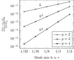
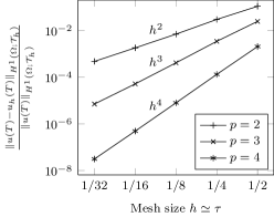
Figure 1: Relative errors in approximating the solution of the problem of section 8.1 using uniform meshes and time partitions with $\tau\simeq h$ and $p=q+1$. It is seen that the optimal convergence rates ${\lvert\kern-1.07639pt\lvert\kern-1.07639pt\lvert u-u_{h}\rvert\kern-1.07639pt\rvert\kern-1.07639pt\rvert}_{h}\simeq h^{p-1}+\tau^{q}$ are achieved. The final time error, as measured in the broken $H^{1}$-norm, also converges with the optimal rate $\lVert u(T)-u_{h}(T)\rVert_{H^{1}\left(\varOmega;\mathcal{T}_{h}\right)}\simeq h^{p}$.

8.2 Second experiment

In section 7.2, we considered error bounds for solutions with limited regularity. The significance of these results stems from the fact that the solutions of many parabolic HJB equations possess limited regularity as a result of early-time singularities induced by the initial datum. This difficulty appears even in the simplest special case of the HJB equation (2.3), namely the heat equation: indeed, consider $\partial_{t}u=\varDelta u$ in $\varOmega\times(0,T)$, $\varOmega=(0,1)^{2}$, with homogeneous lateral boundary condition $u=0$ on $\partial\varOmega\times(0,T)$ and initial datum $u_{0}(x,y)\coloneqq x\left(1-x\right)\sin(\pi y)$. Then, the solution is

$$u(x,y,t)=\frac{4}{\pi^{3}}\sum_{k=1}^{\infty}\frac{1-(-1)^{k}}{k^{3}}\exp(-(k^{2}+1)\,\pi^{2}t)\sin(k\,\pi x)\sin(\pi y).$$ (8.3)

It can be shown that for sufficiently small $t>0$ and nonnegative integers $\sigma$ and $\ell$ such that $2\sigma+\ell\geq 3$, we have $\lVert\partial_{t}^{\sigma}u\rVert_{X_{\ell}}^{2}\simeq t^{-(2\sigma+\ell-5/2)}$, with the constants of these lower and upper bounds both depending on $\sigma$ and $\ell$, but not on $t$. Therefore, $u\notin H^{1}(I;H)$, rather $u\in H^{7/4-\delta}(I;L^{2}(\varOmega))\cap H^{5/4-\delta}(I;H^{1}_{0}(\varOmega))\cap H^{3/4-\delta}(I;H)$ for arbitrarily small $\delta>0$. It is noted that a linear problem is chosen here so that the solution may be found explicity through (8.3). Nevertheless, this example exhibits many features that are typical of more general parabolic problems, so that the following results remain relevant to more general HJB equations.

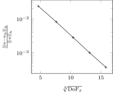
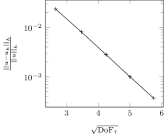
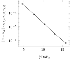
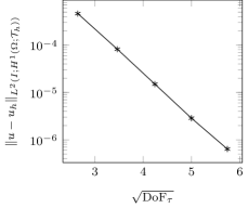
Figure 2: Geometrically-graded spatial meshes used in conjunction with the geometrically-graded temporal meshes for the problem of section 8.2. From left to right, the meshes are those used for the first, third and fifth computations. The corresponding number of spatial degrees of freedom $\mathrm{DoF}_{x}$ are respectively $100$, $1128$, and $3980$.

Figure 3: Exponential convergence rates under $hp$-$\tau q$ refinement for the problem of section 8.2. The errors in the norms ${\lvert\kern-1.07639pt\lvert\kern-1.07639pt\lvert\cdot\rvert\kern-1.07639pt\rvert\kern-1.07639pt\rvert}_{h}$ and $\lVert\cdot\rVert_{L^{2}(I;H^{1}(\varOmega;\mathcal{T}_{h}))}$ are plotted against $\sqrt[3]{\mathrm{DoF}_{x}}$ and $\sqrt{\mathrm{DoF}_{\tau}}$, where $\mathrm{DoF}_{x}$ is the number of spatial degrees of freedom and $\mathrm{DoF}_{\tau}$ is the number of temporal degrees of freedom. Exponential convergence rates of the form of (8.4) are confirmed.

Despite the limited regularity of the solution, accurate results can be obtained by using geometrically-graded time partitions with varying temporal polynomial degrees; see Schotzau2000 . Specifically, a combination of $\tau q$-refinement in time and $hp$-refinement in space can lead to a convergence rate

$${\lvert\kern-1.07639pt\lvert\kern-1.07639pt\lvert u-u_{h}\rvert\kern-1.07639pt\rvert\kern-1.07639pt\rvert}_{h}\lesssim\exp(-c_{1}\sqrt[3]{\mathrm{DoF}_{x}})+\exp(-c_{2}\sqrt{\mathrm{DoF}_{\tau}}),$$ (8.4)

where $\mathrm{DoF}_{x}\coloneqq\operatorname{dim}V_{h,\mathbf{p}}$, where $\mathrm{DoF}_{\tau}=\sum_{n=1}^{N}(q_{n}+1)$ is the number of degrees of freedom of the temporal finite element space, and where $c_{1}$ and $c_{2}$ are positive constants. We give here an experimental confirmation of these expectations.

The method is applied on a sequence of geometrically-graded partitions $\{\mathcal{J}_{\tau}\}_{\tau}$ constructed as follows. Let $T=0.05$, and let $t_{n}=\sigma^{N-n}\,T$ for $n=1,\dots,N$, for a chosen $\sigma\in(0,1)$, and $N=2,\dots,6$. As suggested in Schotzau2000 , we choose $\sigma=0.2$. The temporal polynomial degrees are linearly increasing with $n$, with $q_{n}\coloneqq n+1$. We choose $T$ to be small, because in practice it is natural to use $\tau q$-refinement on a small initial time segment, and then apply uniform or spectral refinement on the remaining time interval, see Schotzau2000 . The spatial meshes are defined as follows: starting with a regular partition of $\varOmega$ into four quadrilateral elements, for each successive computation, we refine the meshes geometrically towards the boundary, thereby leading to the meshes given in Figure 3. The polynomial degrees $p_{K}\geq 3$ are chosen to be linearly increasing away from the boundary.

Figure 3 presents the resulting errors in the norms ${\lvert\kern-1.07639pt\lvert\kern-1.07639pt\lvert\cdot\rvert\kern-1.07639pt\rvert\kern-1.07639pt\rvert}_{h}$ and $\lVert\cdot\rVert_{L^{2}(I;H^{1}(\varOmega;\mathcal{T}_{h}))}$, plotted against $\sqrt[3]{\mathrm{DoF}_{x}}$ and $\sqrt{\mathrm{DoF}_{\tau}}$. It is found that the convergence rates of (8.4) are attained, with higher accuracies being achieved in lower order norms. These results show the computational efficiency of the method for problems with limited regularity.

9 Conclusion

We have introduced and analysed a fully-discrete $hp$- and $\tau q$-version DGFEM for parabolic HJB equations with Cordes coefficients. The method is consistent and unconditionally stable, with proven convergence rates. The numerical experiments demonstrated the efficiency and accuracy of the method on problems with strongly anisotropic diffusion coefficients, and illustrated exponential convergence rates for solutions with limited regularity under $hp$- and $\tau q$-refinement.

Appendix A Approximation theory

A.1 Trace theorem for Besov spaces

We will show that, for a suitable domain $K\subset\mathbb{R}^{d}$, functions in the Besov space $B^{1/2}_{2,1}(K)$ have traces in $L^{2}(\partial K)$. Recall the discrete form of the J-method of interpolation of function spaces Adams2003 : a function $u\in L^{2}(K)$ belongs to $B^{1/2}_{2,1}(K)$ if and only if there exists a sequence $\{u_{i}\}_{i\in\mathbb{Z}}\subset H^{1}(K)$, such that $u=\sum_{i\in\mathbb{Z}}u_{i}$, where the series converges absolutely in $L^{2}(K)$, and such that the sequence $\{2^{-i/2}J(2^{i},u_{i})\}_{i\in\mathbb{Z}}\in\ell^{1}$, where $J(t,v)\coloneqq\max\{\lVert v\rVert_{L^{2}(K)},t\lVert v\rVert_{H^{1}(K)}\}$. Moreover, we may define a norm on $B^{1/2}_{2,1}(K)$ by

$$\lVert u\rVert_{B^{1/2}_{2,1}(K)}\coloneqq\inf\left\{\lVert\{2^{-i/2}J(2^{i},u_{i})\}_{i\in\mathbb{Z}}\rVert_{\ell^{1}},\,u=\sum\nolimits_{i\in\mathbb{Z}}u_{i},\;u_{i}\in H^{1}(K)\right\}.$$ (A.1)

Also, for any such sequence, we have

$$\lim_{m\rightarrow\infty}\lVert u-\sum\nolimits_{\lvert i\rvert\leq m}u_{i}\rVert_{B^{1/2}_{2,1}(K)}\leq\lim_{m\rightarrow\infty}\sum_{\lvert i\rvert>m}2^{-i/2}J(2^{i},u_{i})=0.$$ (A.2)

Hence $H^{1}(K)$ is dense in $B^{1/2}_{2,1}(K)$.

It is sometimes problematic to work with the infinite series representation of a function in the Besov space $B^{1/2}_{2,1}(K)$, as a result of questions concerning convergence of the series in appropriate norms. The following lemma is a key ingredient of our proof of the Trace Theorem, and shows that it is possible to work with representations by finite sums of functions in the dense subspace $H^{1}(K)$.

Lemma 7

Let $K\subset\mathbb{R}^{d}$ be a domain. Then, for each $u\in H^{1}(K)$, there exists a positive integer $m$ and a finite set $\{u_{i}\}_{\lvert i\rvert\leq m}\subset H^{1}(K)$, with $u=\sum_{\lvert i\rvert\leq m}u_{i}$, and

$$\sum_{\lvert i\rvert\leq m}2^{-i/2}J(2^{i},u_{i})\lesssim\lVert u\rVert_{B^{1/2}_{2,1}(K)},$$ (A.3)

where the constant is independent of all other quantities.

Proof

Since the case $u=0$ is trivial, we assume that $u\neq 0$. Since $H^{1}(K)$ is embedded in $B^{1/2}_{2,1}(K)$, there exists a sequence $\{v_{i}\}_{i\in\mathbb{Z}}\subset H^{1}(K)$ such that $u=\sum_{i\in\mathbb{Z}}v_{i}$, and such that $\lVert\{2^{-i/2}J(2^{i},v_{i})\}_{i}\rVert_{\ell^{1}}\leq\sqrt{2}\lVert u\rVert_{B^{1/2}_{2,1}(K)}$. Let $m\geq 1$ be the smallest integer such that $\lVert u\rVert_{H^{1}(K)}\leq 2^{m/2}\lVert u\rVert_{B^{1/2}_{2,1}(K)}$. The series $\sum_{i\in\mathbb{Z}}v_{i}$ converges absolutely to $u$ in $L^{2}(K)$, since $\sum_{i\in\mathbb{Z}}\lVert v_{i}\rVert_{L^{2}(K)}\leq\sum_{i\in\mathbb{Z}}2^{-i/2}J(2^{i},v_{i})\leq\sqrt{2}\lVert u\rVert_{B^{1/2}_{2,1}(K)}$. Therefore,

$$\lVert u-\sum\nolimits_{\lvert i\rvert<m}v_{i}\rVert_{L^{2}(K)}\leq\sum\nolimits_{\lvert i\rvert\geq m}\lVert v_{i}\rVert_{L^{2}(K)}$$ (A.4)

$$\qquad\qquad\leq 2^{-m/2}\sum\nolimits_{\lvert i\rvert\geq m}2^{-i/2}J(2^{i},v_{i})\leq 2^{-(m-1)/2}\lVert u\rVert_{B^{1/2}_{2,1}(K)}.$$

$$\sum_{\lvert i\rvert<m}\lVert v_{i}\rVert_{H^{1}(K)}\leq 2^{(m-1)/2}\sum_{\lvert i\rvert<m}2^{i/2}\lVert v_{i}\rVert_{H^{1}(K)}\leq 2^{m/2}\lVert u\rVert_{B^{1/2}_{2,1}(K)}.$$ (A.5)

Now, define $u_{i}\coloneqq v_{i}$ for $\lvert i\rvert<m$, and $u_{-m}\coloneqq u-\sum_{\lvert i\rvert<m}u_{i}$, whilst $u_{i}\coloneqq 0$ otherwise. By hypothesis, $u\in H^{1}(K)$, so $u_{-m}\in H^{1}(K)$, and we have $u=\sum_{\lvert i\rvert\leq m}u_{i}$. It follows from (A.4) that $2^{m/2}\lVert u_{-m}\rVert_{L^{2}(K)}\leq\sqrt{2}\lVert u\rVert_{B^{1/2}_{2,1}(K)}$. The choice of the integer $m$ and the bound (A.5) show that

$$2^{-m/2}\lVert u_{-m}\rVert_{H^{1}(K)}\leq 2^{-m/2}\left(\lVert u\rVert_{H^{1}(K)}+\sum\nolimits_{\lvert i\rvert<m}\lVert v_{i}\rVert_{H^{1}(K)}\right)\leq 2\lVert u\rVert_{B^{1/2}_{2,1}(K)}.$$

Therefore, $2^{m/2}J(2^{-m},u_{-m})\lesssim\lVert u\rVert_{B^{1/2}_{2,1}(K)}$, and we find that (A.3) holds with a constant that is independent of all other quantities, thereby showing that the set $\{u_{i}\}_{\lvert i\rvert\leq m}$ fulfills all of the above claims. ∎

Theorem A.1

Let $\varOmega\subset\mathbb{R}^{d}$ be a bounded Lipschitz polytopal domain, and let $\{\mathcal{T}_{h}\}_{h}$ be a shape-regular sequence of simplicial or parallelepipedal meshes on $\varOmega$. Then, for each $\mathcal{T}_{h}$ and each $K\in\mathcal{T}_{h}$, the trace operator $\gamma\colon H^{1}(K)\rightarrow L^{2}(\partial K)$ has a unique extension to a bounded linear operator on $B^{1/2}_{2,1}(K)$, and there holds

$$\lVert\gamma u\rVert_{L^{2}(\partial K)}\lesssim\lVert u\rVert_{B^{1/2}_{2,1}(K)}+h_{K}^{-1/2}\lVert u\rVert_{L^{2}(K)}\qquad\forall\,u\in B^{1/2}_{2,1}(K).$$ (A.6)

Proof

For an element $K\in\mathcal{T}_{h}$, let $\gamma\colon H^{1}(K)\rightarrow L^{2}(\partial K)$ denote the trace operator. First, we claim that

$$\lVert\gamma u\rVert_{L^{2}(\partial K)}\lesssim\lVert u\rVert_{B^{1/2}_{2,1}(K)}+h_{K}^{-1/2}\lVert u\rVert_{L^{2}(K)}\quad\forall\,u\in H^{1}(K).$$ (A.7)

For a given $u\in H^{1}(K)$, Lemma 7 shows that there exists a finite set $\{u_{i}\}_{\lvert i\rvert\leq m}\subset H^{1}(K)$ such that $u=\sum_{\lvert i\rvert\leq m}u_{i}$, and such that (A.3) holds. Since $\{\mathcal{T}_{h}\}_{h}$ is a shape-regular sequence of simplicial or parallelepipedal meshes, we have the multiplicative trace inequality (c.f. DiPietro2012 ; Monk1999 )

$$\lVert\gamma u\rVert_{L^{2}(\partial K)}\lesssim\left(\lvert u\rvert_{H^{1}(K)}+h_{K}^{-1}\lVert u\rVert_{L^{2}(K)}\right)^{1/2}\lVert u\rVert_{L^{2}(K)}^{1/2}\quad\forall\,u\in H^{1}(K),$$ (A.8)

where the constant depends only the dimension $d$ and the shape-regularity of $\{\mathcal{T}_{h}\}_{h}$. We remark that the multiplicative trace inequality was proven for the case of triangles in two dimensions in Monk1999 , and can be extended to simplices and parallelepipeds in $\mathbb{R}^{d}$, see DiPietro2012 . Let $\overline{u}$ denote the mean-value of $u$ over $K$, and note that $\lVert u-\overline{u}\rVert_{L^{2}(K)}\lesssim h_{K}\lvert u\rvert_{H^{1}(K)}$, see Brenner2008 . Then, $u-\overline{u}=\sum_{\lvert i\rvert\leq m}(u_{i}-\overline{u}_{i})$, and (A.8) implies that

$$\lVert\gamma(u-\overline{u})\rVert_{L^{2}(\partial K)} \lesssim\sum_{\lvert i\rvert\leq m}\left(\lvert u_{i}\rvert_{H^{1}(K)}+h_{K}^{-1}\lVert u_{i}-\overline{u}_{i}\rVert_{L^{2}(K)}\right)^{1/2}\lVert u_{i}-\overline{u}_{i}\rVert^{1/2}_{L^{2}(K)}$$ (A.9)

$$\lesssim\sum_{\lvert i\rvert\leq m}\lvert u_{i}\rvert_{H^{1}(K)}^{1/2}\lVert u_{i}\rVert_{L^{2}(K)}^{1/2}$$

$$\lesssim\sum_{\lvert i\rvert\leq m}2^{-i/2}\lVert u_{i}\rVert_{L^{2}(K)}+2^{i/2}\lVert u_{i}\rVert_{H^{1}(K)}$$

$$\lesssim\sum_{\lvert i\rvert\leq m}2^{-i/2}J(2^{i},u_{i})\lesssim\lVert u\rVert_{B^{1/2}_{2,1}(K)}.$$

It is also easily found that $\lVert\gamma\overline{u}\rVert_{L^{2}(\partial K)}\lesssim h_{K}^{-1/2}\lVert u\rVert_{L^{2}(K)}$. Therefore, the bound (A.7) follows from the above bounds and the triangle inequality. Thus, the trace operator $\gamma$ is uniformly bounded in the norm of $B^{1/2}_{2,1}(K)$ over the space $H^{1}(K)$, which is densely embedded in $B^{1/2}_{2,1}(K)$. Hence, $\gamma$ has a unique extension to a bounded linear operator $\gamma\colon B^{1/2}_{2,1}(K)\rightarrow L^{2}(\partial K)$, and (A.6) holds. ∎

In the following, we will often omit any explicit reference to the trace operator $\gamma$. For example, we shall write $\lVert u\rVert_{L^{2}(\partial K)}$ rather than $\lVert\gamma u\rVert_{L^{2}(\partial K)}$.

A.2 Polynomial approximation in Sobolev spaces

We recall the results from Babuvska1987a . For a positive integer $d$ and a nonnegative integer $p$, let $\mathcal{P}_{p}$ denote the space of real valued polynomials on $\mathbb{R}^{d}$ with either partial or total degree at most $p$.

Lemma 8

For a nonnegative integer $p$ and $\rho\in\mathbb{R}_{>0}$, a function $u\colon(-\rho,\rho)\rightarrow\mathbb{R}$ is an algebraic polynomial of degree at most $p$ if and only if the function $V\colon\xi\mapsto u(\rho\sin\xi)$ is a trigonometric polynomial of degree at most $p$.

Proof

Suppose that $u$ is an algebraic polynomial of degree at most $p$. Then it is easily found that $V$ is a trigonometric polynomial of degree at most $p$. To show the converse, suppose that $V$ is a trigonometric polynomial of degree at most $p$. Observe that $V$ is necessarily symmetric about $\pm\pi/2$, and thus we have, for any $k\geq 0$,

$$\int_{-\pi}^{\pi}V(\xi)\sin(2k\xi)\,\mathrm{d}\xi=0, \int_{-\pi}^{\pi}V(\xi)\cos(\left(2k+1\right)\xi)\,\mathrm{d}\xi=0.$$ (A.10)

Indeed, the first identity in (A.10) is found by writing

$$\begin{split}\int_{-\pi}^{\pi}v(\xi)\sin(2k\xi)\,\mathrm{d}\xi&=\int_{0}^{\pi}\left(v(\xi)-v(-\xi)\right)\sin(2k\xi)\,\mathrm{d}\xi\\ &=(-1)^{k}\int_{-\pi/2}^{\pi/2}\left(v(\tfrac{\pi}{2}+\delta)-v(-\tfrac{\pi}{2}+\delta)\right)\sin(2k\delta)\,\mathrm{d}\delta,\end{split}$$ (A.11)

and by noting that the right-hand side of (A.11) is the integral of an odd function over an interval centred about $\delta=0$, as a result of the symmetry of $V$. The proof of the second identity in (A.10) is analogous.

Since $V$ is a trigonometric polynomial of degree at most $p$, it follows from (A.10) that

$$V(\xi)=\sum_{1\leq 2k+1\leq p}a_{k}\sin(\left(2k+1\right)\xi)+\sum_{0\leq 2k\leq p}b_{k}\cos(2k\xi).$$

For $x\in(-\rho,\rho)$ and $k\geq 0$, define $P_{2k+1}(x)\coloneqq\sin(\left(2k+1\right)\arcsin(x/\rho))$ and $Q_{2k}(x)\coloneqq\cos(2k\arcsin(x/\rho))$. So, for example, $Q_{0}(x)=1$, $P_{1}(x)=x$, and $Q_{2}(x)=1-2x^{2}$. Therefore, $u$ may be written as $u(x)=\sum_{1\leq 2k+1\leq p}a_{k}\,P_{2k+1}(x)+\sum_{0\leq 2k\leq p}b_{k}\,Q_{2k}(x)$. The recurrence relations $P_{2k+1}(x)=P_{2k-1}(x)+2\,x\,Q_{2k}(x)$ and $Q_{2k+2}(x)=2\,Q_{2}(x)\,Q_{2k}(x)-Q_{2k-2}(x)$, for all $k\geq 1$, allow us to deduce that $P_{2k+1}\in\mathcal{P}_{2k+1}$ and that $Q_{2k}\in\mathcal{P}_{2k}$ for each $k\geq 0$, where $\mathcal{P}_{p}$ denotes here the space of univariate polynomials of degree at most $p$. It then follows that $u\in\mathcal{P}_{p}$. ∎

Theorem A.2

Let $Q\subset[-1,1]^{d}$ be either the unit hypercube or the unit simplex in $\mathbb{R}^{d}$, $d\geq 1$. For each integer $p\geq 0$, there exists a linear operator $\varPi^{p}\colon L^{2}(Q)\rightarrow\mathcal{P}_{p}$, with the following properties. There is a constant $C$, independent of $p$, such that

$$\lVert\varPi^{p}u\rVert_{L^{2}(Q)}\leq C\lVert u\rVert_{L^{2}(Q)}\qquad\forall\,u\in L^{2}(Q).$$ (A.12)

For nonnegative integers $j\leq s$, there is a constant $C$, independent of $p$ but dependent on $s$, such that

$$\lVert u-\varPi^{p}u\rVert_{H^{j}(Q)}\leq C(p+1)^{-(s-j)}\lVert u\rVert_{H^{s}(Q)}\qquad\forall\,u\in H^{s}(Q).$$ (A.13)

Proof

Our proof is similar to the one given in Babuvska1987a , except that we also show that generally $u\neq\varPi^{p}u$, even if $u\in\mathcal{P}_{p}$, contrary to what is claimed in Babuvska1987 . First, we momentarily assume that $\mathcal{P}_{p}$ denotes the space of polynomials of partial degree at most $p$. Since $Q$ is a Lipschitz domain, the Stein Extension Theorem Adams2003 shows that there exists a linear total extension operator $E\colon L^{2}(Q)\rightarrow L^{2}(\mathbb{R}^{d})$, such that, for each nonnegative integer $s$, $\lVert Eu\rVert_{H^{s}(\mathbb{R}^{d})}\lesssim\lVert u\rVert_{H^{s}(Q)}$ for all $u\in H^{s}(Q)$. For $\rho\in\mathbb{R}_{>0}$, let $Q(\rho)\coloneqq[-\rho,\rho]^{d}$. Without loss of generality, we may assume that $\operatorname{supp}Eu\subset Q(3/2)$ for every $u\in L^{2}(Q)$. Let $\varPhi$ be the diffeomorphism from $Q(\pi/2)$ to $Q(2)$ defined by $\varPhi(\xi)\coloneqq(2\sin\xi_{1},\dots,2\sin\xi_{d})$. For $u\in L^{2}(Q)$, let $V(\xi)\coloneqq Eu(\varPhi(\xi))$ for $\xi\in\mathbb{R}^{d}$. It follows that $V$ is a $2\pi$-periodic function that is symmetric about each hyperplane $\xi_{i}=\pm\pi/2$, i.e. for any $\xi\in\mathbb{R}^{d}$ such that $\xi_{i}=\pm\pi/2$ and any $\delta\in\mathbb{R}$, we have $V(\xi+\delta\,e_{i})=V(\xi-\delta\,e_{i})$, where $e_{i}$ is the $i$-th unit vector. Since $\operatorname{supp}Eu\subset Q(3/2)$, we may use the symmetry of $V$ to show that, for any integer $s\geq 0$ and any $u\in H^{s}(Q)$, we have $\lVert V\rVert_{H^{s}(Q(\pi))}^{2}=2^{d}\lVert V\rVert_{H^{s}(Q(\pi/2))}^{2}=2^{d}\lVert V\rVert_{H^{s}(\varPhi^{-1}(Q(3/2)))}^{2}$, and therefore we deduce that $\lVert V\rVert_{H^{s}(Q(\pi))}\lesssim\lVert u\rVert_{H^{s}(Q)}$ for all $u\in H^{s}(Q)$ and all integers $s\geq 0$. The function $V$ admits the Fourier expansion $V=\sum_{k\in\mathbb{Z}^{d}}a_{k}\,\mathrm{e}^{\mathrm{i}\,k\cdot\xi}$, where the coefficients $a_{k}\in\mathbb{C}$ satisfy $\overline{a_{k}}=a_{-k}$, for each $k\in\mathbb{Z}^{d}$, because $V$ is real-valued. For an integer $p\geq 0$, define the trigonometric polynomial $V_{p}$ by $V_{p}(\xi)\coloneqq\sum_{\lvert k\rvert_{\infty}\leq p}a_{k}\,\mathrm{e}^{\mathrm{i}\,k\cdot\xi}$. The relation $\overline{a_{k}}=a_{-k}$ shows that

$$V_{p}(\xi)=a_{0}+\sum_{\begin{subarray}{c}k\in\mathbb{N}^{d}\setminus\{0\}\\ \lvert k\rvert_{\infty}\leq p\end{subarray}}\tfrac{1}{2}(a_{k}+\overline{a_{k}})(\mathrm{e}^{\mathrm{i}\,k\cdot\xi}+\mathrm{e}^{-\mathrm{i}\,k\cdot\xi})+\tfrac{1}{2}(a_{k}-\overline{a_{k}})(\mathrm{e}^{\mathrm{i}\,k\cdot\xi}-\mathrm{e}^{-\mathrm{i}\,k\cdot\xi}),$$

thus implying that $V_{p}$ is real-valued. For any integers $j\leq s$, and any $u\in H^{s}(Q)$,

$$\begin{split}\lvert V-V_{p}\rvert_{H^{j}(Q(\pi))}^{2}&\lesssim\sum_{\lvert k\rvert_{\infty}>p}\lvert k\rvert_{\infty}^{2j}\lvert a_{k}\rvert^{2}\lesssim(p+1)^{-2(s-j)}\sum_{k\in\mathbb{Z}^{d}}\lvert k\rvert_{\infty}^{2s}\lvert a_{k}\rvert^{2}\\ &\lesssim(p+1)^{-2(s-j)}\lvert V\rvert_{H^{s}(Q(\pi))}^{2}\lesssim(p+1)^{-2(s-j)}\lVert u\rVert_{H^{s}(Q)}^{2},\end{split}$$ (A.14)

where the constants are independent of $u$ and $p$.

Define the linear map $\varPi^{p}\colon L^{2}(Q)\rightarrow L^{2}_{\mathrm{loc}}(Q(2))$ by $\varPi^{p}u\coloneqq V_{p}\circ\varPhi^{-1}$. Since the mapping $\varPhi\colon Q(\pi/2)\rightarrow Q(2)$ is a diffeomorphism, and since $Q$ is compactly contained in $Q(2)$, we find that $\lVert\varPi^{p}u\rVert_{L^{2}(Q)}^{2}\lesssim\lVert V_{p}\rVert_{L^{2}(Q(\pi/2))}^{2}\leq\lVert V\rVert_{L^{2}(Q(\pi))}^{2}\lesssim\lVert u\rVert_{L^{2}(Q)}^{2}$ for any $u\in L^{2}(Q)$, where the constants are independent of $u$ and $p$, thus giving (A.12). Likewise, (A.13) follows from (A.14) and from $\lVert u-\varPi^{p}u\rVert_{H^{j}(Q)}\lesssim\lVert V-V_{p}\rVert_{H^{j}(Q(\pi))}$.

In order to show that $\varPi^{p}u$ is a polynomial of partial degree at most $p$, it is enough to show that the univariate functions $x_{i}\mapsto\varPi^{p}u(x_{1},\dots,x_{i},\dots,x_{d})$ are polynomials of degree at most $p$, for each $x\in Q(2)$. However, this follows from Lemma 8 because the trigonometric polynomial $V_{p}=\varPi^{p}u\circ\varPhi$ has partial degree at most $p$.

We now show that $\varPi^{p}$ is inexact when applied to polynomials: in general, $u\neq\varPi^{p}u$ is possible for $u\in\mathcal{P}_{p}$. To show this, consider the special case where $d=1$ and $u\equiv 1$. Since $Eu$ is compactly supported on $Q(3/2)$ and is not identically zero, $Eu$ is necessarily not a polynomial of finite degree on $Q(2)$. Since $V(\xi)=Eu(2\sin\xi)$, Lemma 8 shows that $V$ is not a trigonometric polynomial of finite degree, and we also have $\lVert V-1\rVert_{L^{2}(Q(\pi))}>0$. By convergence of Fourier series, there exists $p_{0}\geq 0$ such that for all $p\geq p_{0}$, we have $\lVert V-V_{p}\rVert_{L^{2}(Q(\pi))}<\tfrac{1}{2}\lVert V-1\rVert_{L^{2}(Q(\pi))}$, so that

$$\lVert V_{p}-1\rVert_{L^{2}(Q(\pi))}>\tfrac{1}{2}\lVert V-1\rVert_{L^{2}(Q(\pi))}>0.$$ (A.15)

Since nonzero trigonometric polynomials have at most finitely many roots, $V_{p}$ cannot be identically equal to $1$ on any open subset of $Q(\pi)$, because otherwise $V_{p}$ would have to be identically equal to $1$ on $Q(\pi)$, thereby contradicting (A.15). Therefore, $V_{p}\not\equiv 1\equiv V$ on $\varPhi^{-1}(Q)$, and thus $u\neq\varPi^{p}u$ on $Q$.

Now, we consider the case where $\mathcal{P}_{p}$ denotes the space of polynomials of total degree $p$. Since the space of polynomials of partial degree $k$ is contained in $\mathcal{P}_{p}$ whenever $k\leq p/d$, we may choose $k\leq p/d\leq k+1$, and we find that the projector $\varPi^{k}$ defined above has the required properties.∎

We note that the polynomial inexactness of the Babuška–Suri projector, as defined in Babuvska1987 ; Babuvska1987a , is independent of the choice of the extension operator, since it results from the requirement that the extended functions have compact support. This requirement is not easily avoided, since it is used to obtain the bound $\lVert V\rVert_{H^{s}(Q(\pi))}\lesssim\lVert u\rVert_{H^{s}(Q)}$.

Lemma 9

Let $Q\subset[-1,1]^{d}$ be either the unit hypercube or the unit simplex in $\mathbb{R}^{d}$, $d\geq 1$. For each pair of nonnegative integers $p$ and $m$, there exists a linear operator $\varPi^{m,p}\colon L^{2}(Q)\rightarrow\mathcal{P}_{p}$, the space of polynomials with partial degree at most $p$, such that $\varPi^{m,p}$ has the following properties. If $u$ is a polynomial of total degree at most $\min(m,p)$, then $\varPi^{m,p}u=u$. There exists a constant $C$, independent of $p$ and $m$, such that

$$\lVert\varPi^{m,p}u\rVert_{L^{2}(Q)}\leq C\lVert u\rVert_{L^{2}(Q)}\qquad\forall\,u\in L^{2}(Q).$$ (A.16)

For any nonnegative integer $s$, there is a constant $C$, independent of $p$ but dependent on $s$ and $m$, such that for each nonnegative integer $j\leq s$,

$$\lVert u-\varPi^{m,p}u\rVert_{H^{j}(Q)}\leq C(p+1)^{-(s-j)}\sum_{r=t}^{s}\lvert u\rvert_{H^{r}(Q)}\quad\forall\,u\in H^{s}(Q),$$ (A.17)

where $t\coloneqq\min(s,p+1,m+1)$.

Proof

For nonnegative integers $m$ and $p$, let $\varPi^{p}$ be the Babuška–Suri projector as given by Theorem A.2, and let $\varPi^{\min(m,p)}_{L^{2}}\colon L^{2}(Q)\rightarrow\mathcal{P}_{\min(m,p)}$ denote the $L^{2}$ projection into the space of polynomials of total degree at most $\min(m,p)$. Then, define

$$\varPi^{m,p}u\coloneqq\varPi^{\min(m,p)}_{L^{2}}u+\varPi^{p}\left(u-\varPi^{\min(m,p)}_{L^{2}}u\right),\quad u\in L^{2}(Q).$$ (A.18)

It follows that $\varPi^{m,p}$ is a well-defined linear operator mapping $L^{2}(Q)$ into $\mathcal{P}_{p}$. Since $\varPi^{p}$ is a linear operator, we see that $\varPi^{m,p}$ is exact on the space of polynomials of total degree at most $\min(m,p)$. To show (A.16), we use the triangle inequality

$$\lVert\varPi^{m,p}u\rVert_{L^{2}(Q)}\leq\lVert\varPi^{\min(m,p)}_{L^{2}}u\rVert_{L^{2}(Q)}+\lVert\varPi^{p}\rVert_{L^{2}(Q)\rightarrow L^{2}(Q)}\lVert u-\varPi^{\min(m,p)}_{L^{2}}u\rVert_{L^{2}(Q)},$$ (A.19)

and we note that, by (A.12), $\lVert\varPi^{p}\rVert_{L^{2}(Q)\rightarrow L^{2}(Q)}\leq C$, with $C$ independent of $p$, and that $\lVert\varPi^{\min(m,p)}_{L^{2}}\rVert_{L^{2}(Q)\rightarrow L^{2}(Q)}\leq 1$. Now, let $j\leq s$ be nonnegative integers, and apply (A.13) to obtain

$$\lVert u-\varPi^{m,p}u\rVert_{H^{j}(Q)}\leq C(p+1)^{-(s-j)}\lVert u-\varPi^{\min(m,p)}_{L^{2}}u\rVert_{H^{s}(Q)}\quad\forall\,u\in H^{s}(Q),$$ (A.20)

where $C$ is independent of $p$ and $m$ but dependent on $s$. Since $Q$ is the unit simplex or unit hypercube, the Bramble–Hilbert Lemma Brenner2008 shows that

$$\lVert u-\varPi^{\min(m,p)}_{L^{2}}u\rVert_{H^{s}(Q)}\leq C\sum_{r=t}^{s}\lvert u\rvert_{H^{r}(Q)}\quad\forall\,u\in H^{s}(Q),$$ (A.21)

where $t\coloneqq\min(s,\min(m,p)+1)$ and $C$ depends on $s$, $\min(m,p)$ and on $Q$. Moreover, by considering seperately the cases $p<m$ and $p\geq m$, it is seen that we may choose the constant in (A.21) to depend only on $m$, and not on $p$. We thus obtain (A.17) by combining (A.20) and (A.21), and noting that the constant may be chosen to be independent of $p$. ∎

Definition of fractional order Sobolev spaces

For a domain $K$ and a real number $s>0$ such that $s\in(r,r+1)$ for a nonnegative integer $r$, we define

$$H^{s}(K)\coloneqq\left(H^{r}(K),H^{r+1}(K)\right)_{s-r,2;J}.$$ (A.22)

Here, we use the standard norm on $H^{r}(K)$ when $r$ is an integer. It follows from the Equivalence Theorem Adams2003 that $H^{s}(K)=\left(H^{r}(K),H^{r+1}(K)\right)_{s-r,2;K}$, where the constant in the equivalence of norms depends only on $s$. Also, in view of the Re-iteration Theorem, we note that

$$\left(H^{r}(K),H^{r+1}(K)\right)_{s-r,1;J}\hookrightarrow H^{s}(K)\hookrightarrow\left(H^{r}(K),H^{r+1}(K)\right)_{s-r,\infty;K},$$ (A.23)

where the embedding constants depend only on $s$, see (Adams2003, , Thm. 7.16, Cor. 7.20). We remark that it is important in the following that these constants are independent of the domain $K$.

In the following, $a\lesssim b$ for $a,b\in\mathbb{R}$ means that there exists a constant $C$ such that $a\leq C\,b$, where $C$ is independent of discretisation parameters, such as the element sizes of the meshes and the polynomial degrees of finite element spaces, but otherwise possibly dependent on other fixed quantities, such as the shape-regularity parameters of the mesh, for example.

Theorem A.3

Let $\varOmega\subset\mathbb{R}^{d}$ be a bounded Lipschitz polytopal domain, and let $\{\mathcal{T}_{h}\}_{h}$ be a shape-regular sequence of simplicial or parallelepipedal meshes on $\varOmega$. For each mesh $\mathcal{T}_{h}$, suppose that $h=\max_{K\in\mathcal{T}_{h}}h_{K}$, where $h_{K}\coloneqq\operatorname{diam}K$ for all $K\in\mathcal{T}_{h}$. For each mesh $\mathcal{T}_{h}$, let $\mathbf{m}=(m_{K};\;K\in\mathcal{T}_{h})$ and $\mathbf{p}=(p_{K};\;K\in\mathcal{T}_{h})$ be vectors of nonnegative integers. Then, there exists a sequence of linear operators $\{\varPi^{{\mathbf{m},\mathbf{p}}}_{h}\}_{h}$, such that $\varPi^{{\mathbf{m},\mathbf{p}}}_{h}\colon L^{2}(\varOmega)\rightarrow V_{h,\mathbf{p}}$, with $\varPi^{{\mathbf{m},\mathbf{p}}}_{h}u\rvert_{K}=u\rvert_{K}$ if $u\rvert_{K}$ is a polynomial of total degree at most $\min(m_{K},p_{K})$, and such that, for each $K\in\mathcal{T}_{h}$,

$$\lVert\varPi^{{\mathbf{m},\mathbf{p}}}_{h}u\rVert_{L^{2}(K)}\lesssim\lVert u\rVert_{L^{2}(K)}\qquad\forall\,u\in L^{2}(K).$$ (A.24)

Also, for each $K\in\mathcal{T}_{h}$, $s_{K}\in\mathbb{R}_{\geq 0}$, each nonnegative integer $j\leq s_{K}$ and, if $s_{K}>1/2$, for each multi-index $\beta$, with $\lvert\beta\rvert<s_{K}-1/2$, we have

$$\lVert u-\varPi^{{\mathbf{m},\mathbf{p}}}_{h}u\rVert_{H^{j}(K)} \lesssim\frac{h_{K}^{t_{K}-j}}{(p_{K}+1)^{s_{K}-j}}\lVert u\rVert_{H^{s_{K}}(K)} \forall\,u\in H^{s_{K}}(K),$$ (A.25)

$$\lVert D^{\beta}(u-\varPi^{{\mathbf{m},\mathbf{p}}}_{h}u)\rVert_{L^{2}(\partial K)} \lesssim\frac{h_{K}^{t_{K}-\lvert\beta\rvert-1/2}}{(p_{K}+1)^{s_{K}-\lvert\beta\rvert-1/2}}\lVert u\rVert_{H^{s_{K}}(K)} \forall\,u\in H^{s_{K}}(K),$$ (A.26)

where $t_{K}\coloneqq\min(s_{K},p_{K}+1,m_{K}+1)$.

Proof

Since the meshes $\{\mathcal{T}_{h}\}$ consist of simplices or parallelepipeds, each element $K$ is affine-equivalent to the unit simplex or unit hypercube, with a corresponding affine mapping $F_{K}\colon K\rightarrow Q$. For each $K\in\mathcal{T}_{h}$, define $\hat{u}=u\circ F_{K}^{-1}$ and $\varPi^{{\mathbf{m},\mathbf{p}}}_{h}u\rvert_{K}=\left(\varPi^{m_{K},p_{K}}\hat{u}\right)\circ F_{K}\in\mathcal{P}_{p_{K}}$, where $\varPi^{m_{K},p_{K}}$ is the operator given by Lemma 9. The stability bound (A.24) then follows from the shape-regularity of the mesh and from the bound (A.16) of Lemma 9. Also, for any nonnegative integers $j\leq s$, we have

$$\lVert u-\varPi^{{\mathbf{m},\mathbf{p}}}_{h}u\rVert_{H^{j}(K)}\lesssim\frac{h_{K}^{t_{K}-j}}{(p_{K}+1)^{s_{K}-j}}\lVert u\rVert_{H^{s_{K}}(K)}\quad\forall\,u\in H^{s_{K}}(K),$$ (A.27)

where $t_{K}=\min(s_{K},p_{K}+1,m_{K}+1)$ and where the constant depends only on $s_{K}$, $m_{K}$, on $\max h$ the maximum mesh size over all meshes, on the reference element and on the shape-regularity of $\{\mathcal{T}_{h}\}$. We remark that the additional dependence on $\max h$ stems from the fact that we use the bound $h_{K}^{t_{K}-i}\leq\max h^{j-i}\,h_{K}^{t_{K}-j}$, $i\leq j$, to obtain (A.27). The Exact Interpolation Theorem Adams2003 shows that (A.27) extends to each nonnegative integer $j$ and each nonnegative real number $s_{K}$ such that $j\leq s_{K}$, thus giving (A.25).

We now show (A.26). Let $s_{K}>1/2$ and $\beta$ be a multi-index with $\lvert\beta\rvert<s_{K}-1/2$. First, consider the case where $\lvert\beta\rvert\leq s_{K}-1$. Then, (A.26) follows from (A.25) and from the multiplicative trace inequality (A.8). Now, consider the case where $s_{K}-\lvert\beta\rvert\in(\tfrac{1}{2},1)$. Theorem A.1 shows that, for any $u\in H^{s_{K}}(K)$,

$$\lVert D^{\beta}(u-\varPi^{{\mathbf{m},\mathbf{p}}}_{h}u)\rVert_{L^{2}(\partial K)}\lesssim\lVert D^{\beta}(u-\varPi^{{\mathbf{m},\mathbf{p}}}_{h}u)\rVert_{B^{1/2}_{2,1}(K)}+h_{K}^{-1/2}\lVert u-\varPi^{{\mathbf{m},\mathbf{p}}}_{h}u\rVert_{H^{\lvert\beta\rvert}(K)}.$$

Given (A.25) for the case $j=\lvert\beta\rvert$, we can obtain (A.26) provided that we can show that, for any $u\in H^{s_{K}}(K)$,

$$\lVert D^{\beta}(u-\varPi^{{\mathbf{m},\mathbf{p}}}_{h}u)\rVert_{B^{1/2}_{2,1}(K)}\lesssim\frac{h_{K}^{t_{K}-\lvert\beta\rvert-1/2}}{(p_{K}+1)^{s_{K}-\lvert\beta\rvert-1/2}}\lVert u\rVert_{H^{s_{K}}(K)}.$$ (A.28)

The Exact Interpolation Theorem and (A.27) show that $\lVert u-\varPi^{{\mathbf{m},\mathbf{p}}}_{h}u\rVert_{H^{s_{K}}(K)}\lesssim\lVert u\rVert_{H^{s_{K}}(K)}$ for any $u\in H^{s_{K}}(K)$. The Re-iteration Theorem Adams2003 shows that

$$B^{1/2}_{2,1}(K)=\left(L^{2}(K),H^{s_{K}-\lvert\beta\rvert}(K)\right)_{\lambda,1;J},$$

where $\lambda\coloneqq\tfrac{1}{2(s_{K}-\lvert\beta\rvert)}$, and where the constant in the equivalence of norms depends only on $s_{K}-\lvert\beta\rvert$. Therefore, for any $u\in H^{s_{K}}(K)$, there holds

$$\lVert D^{\beta}(u-\varPi^{{\mathbf{m},\mathbf{p}}}_{h}u)\rVert_{B^{1/2}_{2,1}(K)}\lesssim\left(\frac{h_{K}^{t_{K}-\lvert\beta\rvert}}{(p_{K}+1)^{s_{K}-\lvert\beta\rvert}}\right)^{1-\lambda}\lVert u\rVert_{H^{s_{K}}(K)}.$$

Since $t_{K}\leq s_{K}$, we have $(t_{K}-\lvert\beta\rvert)(1-\lambda)\geq t_{K}-\lvert\beta\rvert-1/2$, and therefore we deduce (A.28) and (A.26). ∎

A.3 Polynomial approximation in Bochner spaces

To simplify the notation in the following approximation results, let the spaces $\{X_{\ell}\}_{\ell=0}^{2}$ be defined by

$$X_{0} \coloneqq L^{2}(\varOmega), X_{1} \coloneqq H^{1}_{0}(\varOmega), X_{2} \coloneqq H=H^{2}(\varOmega)\cap H^{1}_{0}(\varOmega).$$

The approximation theory for Sobolev spaces can be extended to Bochner spaces as follows.

Lemma 10

Let $I$ be an open interval and let $\varOmega\subset\mathbb{R}^{d}$ be a bounded convex domain. Let $\{\psi_{k}\}_{k=1}^{\infty}\subset H\coloneqq H^{2}(\varOmega)\cap H^{1}_{0}(\varOmega)$ be an orthonormal basis of $L^{2}(\varOmega)$, such that $\{\psi_{k}\}_{k=1}^{\infty}$ is also an orthogonal basis of $H^{1}_{0}(\varOmega)$ and of $H$, which satisfies

$$\int_{\varOmega}\psi_{k}\,\psi_{j}\,\mathrm{d}x =\delta_{kj}, \int_{\varOmega}\nabla\psi_{k}\cdot\nabla\psi_{j}\,\mathrm{d}x =\lambda_{k}\,\delta_{kj}, \int_{\varOmega}\varDelta\psi_{k}\,\varDelta\psi_{j}\,\mathrm{d}x =\lambda_{k}^{2}\,\delta_{kj},$$

where $\lambda_{k}>0$ for eack $k\in\mathbb{N}$. Then, for any $\ell\in\{0,1,2\}$, and any $u\in L^{2}(I;X_{\ell})$, we have $u=\sum_{k=1}^{\infty}u_{k}\,\psi_{k}$, where $u_{k}(t)\coloneqq\langle u(t),\psi_{k}\rangle_{L^{2}(\varOmega)}$, and where the series converges in $L^{2}(I;X_{\ell})$. For any integer $s\geq 0$, any $u\in H^{s}(I;X_{\ell})$, we have the generalised Parseval Identity

$$\lvert u\rvert_{H^{s}(I;X_{\ell})}^{2}=\sum_{k=1}^{\infty}\lambda_{k}^{\ell}\,\lvert u_{k}\rvert_{H^{s}(I)}^{2}.$$ (A.29)

Proof

Let $\ell\in\{0,1,2\}$ and let the function $u\in L^{2}(I;X_{\ell})$. Then, $u_{k}$ defined above is a measurable real-valued function, and $\lVert u_{k}(t)\rVert_{L^{2}(I)}\leq\lVert u\rVert_{L^{2}(I;X_{0})}$ for each $k\in\mathbb{N}$. For each $m\in\mathbb{N}$, define the function $v_{m}\in L^{2}(I;X_{2})$ by $v_{m}\coloneqq\sum_{k=1}^{m}u_{k}\,\psi_{k}$. Then, orthogonality of the $\{\psi_{k}\}_{k=1}^{\infty}$ in $X_{\ell}$ implies the Bessel Inequality $\sum_{k=1}^{m}\lambda_{k}^{\ell}\,\lVert u_{k}\rVert_{L^{2}(I)}^{2}=\lVert v_{m}\rVert_{L^{2}(I;X_{\ell})}^{2}\leq\lVert u\rVert_{L^{2}(I;X_{\ell})}^{2}$. It can then be shown that $\{v_{m}\}_{m=1}^{\infty}$ is a Cauchy sequence in $L^{2}(I;X_{\ell})$, with limit denoted by $v$. Moreover, there exists a subsequence of $\{v_{m}\}_{m=1}^{\infty}$ which converges to $v$ in $X_{\ell}$ pointwise almost everywhere on $I$. Thus, it follows from the definition of the functions $v_{m}$ that $\langle v(t),\psi_{k}\rangle_{L^{2}(\varOmega)}=u_{k}(t)=\langle u(t),\psi_{k}\rangle_{L^{2}(\varOmega)}$ for each $k\in\mathbb{N}$, for a.e. $t\in I$, which shows that $v=u$, since $\{\psi_{k}\}_{k=1}^{\infty}$ is an orthonormal basis of $L^{2}(\varOmega)$. This proves that $u=\sum_{k=1}^{\infty}u_{k}\,\psi_{k}$ and shows Parseval’s Identity (A.29) for the case $s=0$. Now, let $s\geq 1$ be an integer, and suppose $u\in H^{s}(I;X_{\ell})$ for some $\ell\in\{0,1,2\}$. Let $\phi\in C^{\infty}_{0}(I)$, and compute $\int_{I}u_{k}\,\partial_{t}^{s}\phi\,\mathrm{d}t=\int_{I}\langle u,\partial_{t}^{s}(\phi\,\psi_{k})\rangle_{L^{2}(\varOmega)}\,\mathrm{d}t=(-1)^{s}\int_{I}\langle\partial_{t}^{s}u,\psi_{k}\rangle_{L^{2}(\varOmega)}\phi\,\mathrm{d}t$. Therefore, the weak derivative $\partial_{t}^{s}u_{k}$ exists in $L^{2}(I)$ and $\partial_{t}^{s}u_{k}=\langle\partial_{t}^{s}u,\psi_{k}\rangle_{L^{2}(\varOmega)}$. So, the generalised Parseval Identity (A.29) for integer $s\geq 1$ is found by applying (A.29) for $s=0$ to the function $\partial_{t}^{s}u$.∎

Recall that for a Banach space $X$ and a nonnegative integer $q$, the space of univariate $X$-valued polynomials of degree at most $q$ is denoted by $\mathcal{Q}_{q}(X)$.

Lemma 11

Let $\varOmega\subset\mathbb{R}^{d}$ be a bounded convex domain, let $I$ be an open interval of length $\tau_{0}$, and let $r$ and $q$ be nonnegative integers. Then, for each open interval $J\subset I$ of length $\tau\leq\tau_{0}$, there exists a linear operator $\varPi^{r,q}_{\tau}$ defined on $L^{2}(J;L^{2}(\varOmega))$ with the following properties. The operator $\varPi^{r,q}_{\tau}\colon L^{2}(J;X_{\ell})\rightarrow\mathcal{Q}_{q}(X_{\ell})$ for each $\ell\in\{0,1,2\}$, with $\varPi^{r,q}_{\tau}u=u$ if $u\in\mathcal{Q}_{\min(r,q)}(X_{\ell})$. Furthermore,

$$\lVert\varPi^{r,q}_{\tau}u\rVert_{L^{2}(J;X_{\ell})}\lesssim\lVert u\rVert_{L^{2}(J;X_{\ell})}\quad\forall\,u\in L^{2}(J;X_{\ell}),$$ (A.30)

where the constant is independent of all quantities. For any real $\sigma\geq 0$ and any nonnegative integer $j\leq\sigma$,

$$\lvert u-\varPi^{r,q}_{\tau}u\rvert_{H^{j}(J;X_{\ell})}\lesssim\frac{\tau^{\varrho-j}}{(q+1)^{\sigma-j}}\lVert u\rVert_{H^{\sigma}(J;X_{\ell})}\quad\forall\,u\in H^{\sigma}(J;X_{\ell}),$$ (A.31)

where $\varrho\coloneqq\min(\sigma,r+1,q+1)$, and where the constant depends only on $\tau_{0}$, $\sigma$ and $r$.

Proof

Let $u\in L^{2}(J;L^{2}(\varOmega))$ and define $u_{k}$, $k\in\mathbb{N}$, as in Lemma 10. Let $F$ denote the affine mapping from the reference element $(-1,1)$ to $J$. Then, for each $k\in\mathbb{N}$, define the univariate real-valued polynomial $\varPi^{r,q}_{\tau}u_{k}\coloneqq\left(\varPi^{r,q}\hat{u}_{k}\right)\circ F^{-1}$, where $\hat{u}_{k}\coloneqq u_{k}\circ F$, and where $\varPi^{r,q}$ is the approximation operator on the reference element given by Lemma 9 for $d=1$. For each $k\in\mathbb{N}$, $\varPi^{r,q}_{\tau}u_{k}$ has degree at most $q$. It follows from Lemma 9 that $\lVert\varPi^{r,q}_{\tau}u_{k}\rVert_{L^{2}(J)}\lesssim\lVert u_{k}\rVert_{L^{2}(J)}$, where the constant is independent of all other quantities. Therefore, Lemma 10 implies that $\varPi^{r,q}_{\tau}u\coloneqq\sum_{k=1}^{\infty}\varPi^{r,q}_{\tau}u_{k}\,\psi_{k}$ is well-defined in $L^{2}(J,L^{2}(\varOmega))$. Furthermore, if $u\in L^{2}(J;X_{\ell})$ for some $\ell\in\{0,1,2\}$, then Lemma 10 shows that

$$\lVert\varPi^{r,q}_{\tau}u\rVert_{L^{2}(J;X)}^{2}=\sum_{k=1}^{\infty}\lambda_{k}^{\ell}\lVert\varPi^{r,q}_{\tau}u_{k}\rVert_{L^{2}(J)}^{2}\lesssim\lVert u\rVert_{L^{2}(J;X_{\ell})}^{2},$$

where the constant is independent of all quantities, thereby showing (A.30). This also implies that $\varPi^{{\mathbf{r},\mathbf{q}}}_{\tau}\colon L^{2}(J;X_{\ell})\rightarrow\mathcal{Q}_{q}(X_{\ell})$ for each $\ell\in\{0,1,2\}$. Moreover, if $u\in\mathcal{Q}_{\min(r,q)}(X_{\ell})$, then $\varPi^{r,q}_{\tau}u_{k}=u_{k}$ for each $k\in\mathbb{N}$ by Lemma 9, which implies that $\varPi^{r,q}_{\tau}u=u$ by Lemma 10.

Let $j\leq\sigma$ be nonnegative integers and let $u\in H^{\sigma}(J;X_{\ell})$ for some $\ell\in\{0,1,2\}$. Then, Lemmas 9 and 10 imply that

$$\lvert u-\varPi^{r,q}_{\tau}u\rvert_{H^{j}(J;X_{\ell})}^{2}=\sum_{k=1}^{\infty}\lambda_{k}^{\ell}\,\lvert u_{k}-\varPi^{r,q}_{\tau}u_{k}\rvert_{H^{j}(J)}^{2}\\ \lesssim\sum_{\nu=\varrho}^{\sigma}\frac{\tau^{2(\nu-j)}}{(q+1)^{2(\sigma-j)}}\sum_{k=1}^{\infty}\lambda_{k}^{\ell}\,\lvert u_{k}\rvert_{H^{\nu}(J)}^{2}\lesssim\frac{\tau^{2(\varrho-j)}\max\left(1,\tau_{0}^{2(\sigma-\varrho)}\right)}{(q+1)^{2(\sigma-j)}}\sum_{\nu=\varrho}^{\sigma}\lvert u\rvert_{H^{\nu}(J;X_{\ell})}^{2},$$ (A.32)

where the constant depends only on $\sigma$ and $r$, thereby giving the bound (A.31) for the case where $\sigma$ is an integer. Therefore, the bound (A.31) for general $\sigma\in\mathbb{R}_{\geq 0}$ follows from (A.32) and the theory of interpolation of function spaces. ∎

References

- (1) Adams, R.A., Fournier, J.F.: Sobolev spaces, Pure and Applied Mathematics, vol. 140, second edition. Elsevier (2003)
- (2) Akrivis, G., Makridakis, C.: Galerkin time-stepping methods for nonlinear parabolic equations. M2AN Math. Model. Numer. Anal. 38(2), 261–289 (2004).
- (3) Babuška, I., Suri, M.: The - version of the finite element method with quasi-uniform meshes. RAIRO Modél. Math. Anal. Numér. 21(2), 199–238 (1987).
- (4) Babuška, I., Suri, M.: The optimal convergence rate of the -version of the finite element method. SIAM J. Numer. Anal. 24(4), 750–776 (1987).
- (5) Barles, G., Souganidis, P.: Convergence of approximation schemes for fully nonlinear second-order equations. Asymptotic Anal. 4(3), 271–283 (1991).
- (6) Bonnans, J.F., Zidani, H.: Consistency of generalized finite difference schemes for the stochastic HJB equation. SIAM J. Numer. Anal. 41(3), 1008–1021 (2003).
- (7) Brenner, S.C., Scott, L.R.: The mathematical theory of finite element methods, Texts in Applied Mathematics, vol. 15, third edition. Springer, New York (2008).
- (8) Camilli, F., Falcone, M.: An approximation scheme for the optimal control of diffusion processes. RAIRO Modél. Math. Anal. Numér. 29(1), 97–122 (1995).
- (9) Cordes, H.O.: Über die erste Randwertaufgabe bei quasilinearen differentialgleichungen zweiter ordnung in mehr als zwei variablen. Math. Ann. 131, 278–312 (1956).
- (10) Crandall, M.G., Lions, P.L.: Convergent difference schemes for nonlinear parabolic equations and mean curvature motion. Numer. Math. 75(1), 17–41 (1996).
- (11) Debrabant, K., Jakobsen, E.R.: Semi-Lagrangian schemes for linear and fully nonlinear diffusion equations. Math. Comp. 82(283), 1433–1462 (2013).
- (12) Di Pietro, D.A., Ern, A.: Mathematical aspects of discontinuous Galerkin methods, Mathématiques & Applications (Berlin), vol. 69. Springer, Heidelberg (2012).
- (13) Fleming, W.H., Soner, H.M.: Controlled Markov processes and viscosity solutions, Stochastic Modelling and Applied Probability, vol. 25, second edition. Springer, New York (2006).
- (14) Gilbarg, D., Trudinger, N.S.: Elliptic partial differential equations of second order. Classics in Mathematics. Springer-Verlag, Berlin (2001).
- (15) Grisvard, P.: Elliptic problems in nonsmooth domains, Classics in Applied Mathematics, vol. 69. SIAM, Philadelphia (2011).
- (16) Jensen, M., Smears, I.: On the convergence of finite element methods for Hamilton–Jacobi–Bellman equations. SIAM J. Numer. Anal. 51(1), 137–162 (2013).
- (17) Kushner, H.J.: Numerical methods for stochastic control problems in continuous time. SIAM J. Control Optim. 28(5), 999–1048 (1990).
- (18) Maugeri, A., Palagachev, D.K., Softova, L.G.: Elliptic and parabolic equations with discontinuous coefficients, Mathematical Research, vol. 109. Wiley-VCH Verlag Berlin GmbH, Berlin (2000).
- (19) Monk, P., Süli, E.: The adaptive computation of far-field patterns by a posteriori error estimation of linear functionals. SIAM J. Numer. Anal. 36(1), 251–274 (1999).
- (20) Mozolevski, I., Süli, E., Bösing, P.R.: -version a priori error analysis of interior penalty discontinuous Galerkin finite element approximations to the biharmonic equation. J. Sci. Comput. 30(3), 465–491 (2007).
- (21) Renardy, M., Rogers, R.C.: An introduction to partial differential equations, Texts in Applied Mathematics, vol. 13, second edition. Springer-Verlag, New York (2004).
- (22) Schötzau, D., Schwab, C.: Time discretization of parabolic problems by the -version of the discontinuous Galerkin finite element method. SIAM J. Numer. Anal. 38(3), 837–875 (2000).
- (23) Smears, I., Süli, E.: Discontinuous Galerkin finite element approximation of nondivergence form elliptic equations with Cordes coefficients. SIAM J. Numer. Anal. 51, 2088–2106 (2013).
- (24) Smears, I., Süli, E.: Discontinuous Galerkin finite element approximation of Hamilton–Jacobi–Bellman equations with Cordes coefficients. SIAM J. Numer. Anal. 52(2), 993–1016 (2014).
- (25) Thomée, V.: Galerkin finite element methods for parabolic problems, Springer Series in Computational Mathematics, vol. 25, second edition. Springer-Verlag, Berlin (2006).
- (26) Wloka, J.: Partial differential equations. Cambridge University Press, Cambridge (1987).