Complete wetting near an edge of a rectangular-shaped substrate

Abstract

We consider fluid adsorption near a rectangular edge of a solid substrate that interacts with the fluid atoms via long range (dispersion) forces. The curved geometry of the liquid-vapour interface dictates that the local height of the interface above the edge $\ell_{E}$ must remain finite at any subcritical temperature, even when a macroscopically thick film is formed far from the edge. Using an interfacial Hamiltonian theory and a more microscopic fundamental measure density functional theory (DFT), we study the complete wetting near a single edge and show that $\ell_{E}(0)-\ell_{E}(\delta\mu)\sim\delta\mu^{\beta_{E}^{co}}$, as the chemical potential departure from the bulk coexistence $\delta\mu=\mu_{s}(T)-\mu$ tends to zero. The exponent $\beta_{E}^{co}$ depends on the range of the molecular forces and in particular $\beta_{E}^{co}=2/3$ for three-dimensional systems with van der Waals forces. We further show that for a substrate model that is characterised by a finite linear dimension $L$, the height of the interface deviates from the one at the infinite substrate as $\delta\ell_{E}(L)\sim L^{-1}$ in the limit of large $L$. Both predictions are supported by numerical solutions of the DFT.

I Introduction

It is well known that the adsorption properties of solid substrates strongly depend on the substrate geometry. In particular, the nature of pertinent surface phase transitions on non-planar substrates may qualitatively differ from those on planar walls. The surface geometry can have a profound influence on the location of the phase transitions, their order, and the values of the critical exponents, and it can even induce entirely new interfacial phase transitions and fluctuation effects cacamo ; bonn ; saam ; hauge ; rejmer ; wood ; nature ; silvestre . Recent theoretical studies also have revealed new examples of surprising connections between adsorption in different geometries cov1 ; cov2 . These findings are not only interesting in their own rights but also have useful and far-reaching consequences for applications that require the design of modified surfaces, whose adsorption properties can be sensitively controlled at the nanoscale. Indeed, recent advances in nano-lithography have opened up an entirely new area of research with exciting implications for modern technologies whitesides ; quere ; rauscher that address the properties of fluids that are geometrically constrained to a molecular scale. Examples of the products of this sort of innovation include self-cleaning materials selfclean , responsive polymer brushes brush or “lab-on-a-chip” devices chips .

A prerequisite to these applications is a detailed description of fluid adsorption on structures of the most fundamental non-planar geometries. This paper focuses on the adsorption of a simple fluid near a substrate edge. In the simplest case of a single edge, the substrate geometry can be characterised by an internal angle $\phi<\pi$, where two semi-infinite planes meet. This (convex) object should be distinguished from a (concave) linear wedge model, because the fluid behaviours on these two substrates are strikingly different. While the wedge geometry promotes fluid condensation and shifts the temperature where macroscopic coverage occurs below the wetting temperature $T_{w}$ of a corresponding planar wall rejmer ; wood , the presence of the substrate edge implies that the height of the liquid-vapour interface above the edge $\ell_{E}$ remains finite at any subcritical temperature, even when the interface far from the edge $\ell_{\pi}$ unbinds from the wall. This suppression occurs because of the surface free energy cost, that must be paid for interface bending above the edge, similarly to adsorption on a spherical wall where the growth of an adsorbed film is restricted by the Laplace pressure arising from the curved liquid-vapour interface stewart ; nold .

A proper understanding of how the presence of the edge affects the wetting properties of the wall is important to obtain a comprehensive picture of adsorption on structured (or sculpted) surfaces. Recently, theoretical and experimental studies have shown that a planar wall etched with an array of rectangular grooves exhibits more adsorption regimes than the simple flat wall cov2 ; bruschi1 ; bruschi2 ; tasin ; hofmann ; checco ; mal . A recent density functional (DFT) study mal revealed that hydrophilic grooved surfaces experience the wetting transition at temperature $T>T_{w}$, which is in contrast with the predictions based on macroscopic approaches, such as the Wenzel model, predicting that surface corrugation promotes the surface’s wetting properties quere . Furthermore, the regimes that are characterised by the formation of a laterally inhomogeneous film with the interface pinned at the groove edges and followed by a discontinuous unbending unbending of the interface have been observed. In these cases, the presence of the groove edges plays a crucial role and the explanation of these phenomena is incomplete without our knowledge of what occurs in the immediate vicinity of an isolated edge.

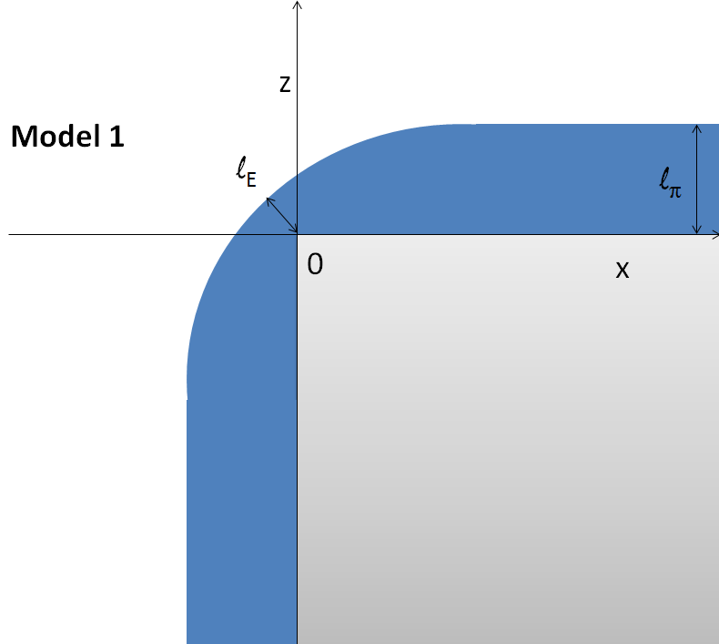
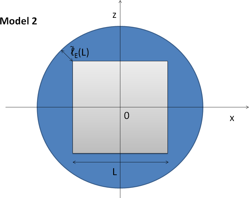
Figure 1: Left: A sketch of Model 1 in the $x$-$z$ projection. The liquid film thickness above the edge of the substrate is $\ell_{E}$, while far away from the edge the film thickness approaches the value $\ell_{\pi}$ corresponding to an adsorbed layer above a planar wall. Right: A sketch of Model 2 in the $x$-$z$ projection. The liquid film thickness above each of the four edges of the substrate is $\ell_{E}(L)$, which now depends on the linear dimension of the wall $L$. In both cases, the wall is infinitely long along the Cartesian $y$-coordinate.

A study by Parry et al. parry_apex provides a description of the adsorption near an edge that focuses on the limit of $\phi\to\pi$ and shows a connection between complete wetting near a shallow edge and critical wetting on a planar wall. Here, motivated by the previously mentioned studies of rectangular grooves, we adopt a model with a long-range wall-fluid potential and fix the internal angle to $\phi=\pi/2$. We seek for the dependence of the local height of the adsorbed liquid film above the edge $\ell_{E}$ on the chemical potential offset from saturation $\delta\mu\equiv\mu_{\rm s}(T)-\mu$ when the bulk coexistence is approached from below, $\delta\mu\to 0^{+}$. To this end, we consider two substrate models, as schematically pictured in Fig. 1. Using Model 1, the effective Hamiltonian theory reveals that

$$\ell_{E}(0)-\ell_{E}(\delta\mu)\sim\delta\mu^{\beta_{E}^{co}}+{\cal{O}}(\delta\mu)\,,$$ (1)

as $\delta\mu\to 0^{+}$ with a non-universal critical exponent $\beta_{E}^{co}=p/(p+1)$, where the parameter $p$ characterises a decay of the binding potential far from the edge $W(\ell)\sim\ell^{-p}$ (for $\delta\mu=0$). In the most relevant case of (3D) non-retarded van der Waals forces $p=2$, whence $\beta_{E}^{co}=2/3$. In contrast, the next-to-leading term in (1) scales linearly with $\delta\mu$, regardless of the nature of the molecular interaction. We confirm this prediction by the numerical solution of a microscopic DFT. However, for small $\delta\mu$, the requirements on the system size become rather challenging. Therefore, as an alternative, we also consider Model 2 with a finite wall of a square cross-section with a linear dimension $L$ and use scaling arguments to relate the height of the interface above the edge $\ell(L)$ with the wall size:

$$\ell_{E}-\ell_{E}(L)\sim L^{-1}+{\cal{O}}(L^{-\frac{3}{2}})\,,$$ (2)

where all powers now depend on the molecular model and can be expressed in terms of the critical exponents characterising wetting on a planar wall. This prediction is also confirmed by the DFT, whose implementation for Model 2 is rather straightforward.

We conclude this section by briefly recalling some properties of complete wetting on a planar wall for 3D systems with long-range forces (see, e.g., Ref. dietrich ) that are relevant for our purposes. We fix the temperature to a value between the wetting temperature $T_{w}$ and the bulk critical temperature $T_{c}$ and consider the limit $\delta\mu\to 0^{+}$. The mean thickness of the wetting layer $\ell_{\pi}(\delta\mu)$ is driven by the effective interaction (binding potential) between the wall surface and the liquid-vapour interface:

$$W(\ell)=\delta\mu\Delta\rho\ell+B\ell^{-p}+\cdots$$ (3)

where $B>0$ is the Hamaker constant and $\Delta\rho=\rho_{l}-\rho_{v}$ is the difference between the liquid density and the vapour density at the bulk coexistence. The global minimum of $W(\ell)$ is at the finite value of $\ell_{\pi}$ for any $\delta\mu>0$, but as $\delta\mu\to 0^{+}$, $\ell_{\pi}$ continuously diverges. The singularity of $W(\ell_{\pi})$ at $\delta\mu=0$ can be characterised by the set of critical exponents, in particular lipowsky :

$$\ell_{\pi}\sim\delta\mu^{-\beta_{s}^{co}}\,,\;\;\;\beta_{s}^{co} = 1/(p+1)\,,$$ (4)

$$\xi_{||}\sim\delta\mu^{-\nu_{||}^{co}}\,,\;\;\;\nu_{||}^{co} = (p+2)/(2p+2)\,,$$ (5)

$$f_{\rm sing}\sim\delta\mu^{2-\alpha_{s}^{co}}\,,\;\;\;\alpha_{s}^{co} = (p+2)/(p+1)\,,$$ (6)

where $\xi_{||}$ is the transverse correlation length, and $f_{\rm sing}$ denotes a singular part of the surface free energy. We recall that the upper critical dimension for complete wetting is $d_{u}<3$ for any finite value of $p$, so that the expressions (4)–(6) are also valid beyond the mean-field approximation in our three-dimensional system lipowsky .

The remainder of the paper is organised as follows. In section 2, we describe our DFT model. An effective Hamiltonian theory and the finite-size scaling arguments are presented in section 3, and their predictions are compared with the DFT in section 4. The results are summarised and discussed in section 5.

II Density Functional Theory

In the classical density functional theory evans79 , the equilibrium density profile minimises the grand potential functional

$$\Omega[\rho]={\cal F}[\rho]+\int{\rm d}{\mathbf{r}}\rho({\bf r})[V({\mathbf{r}})-\mu]\,,$$ (7)

where $\mu$ is the chemical potential, and $V({\mathbf{r}})$ is the external potential. The intrinsic free energy functional ${\cal F}[\rho]$ can be separated into an exact ideal gas contribution and an excess part:

$${\cal F}[\rho]=\beta^{-1}\int{\rm d}{\bf r}\rho({\mathbf{r}})\left[\ln(\rho({\bf r})\Lambda^{3})-1\right]+{\cal F}_{\rm ex}[\rho]\,,$$ (8)

where $\Lambda$ is the thermal de Broglie wavelength and $\beta=1/k_{B}T$ is the inverse temperature. As is common in the modern DFT approaches, the excess part is modelled as a sum of hard-sphere and attractive contributions where the latter is treated in a simple mean-field fashion:

$${\cal F}_{\rm ex}[\rho]={\cal F}_{\rm hs}[\rho]+\frac{1}{2}\int\int{\rm d}{\mathbf{r}}{\rm d}{\mathbf{r}}^{\prime}\rho({\bf r})\rho({\mathbf{r}}^{\prime})u_{\rm a}(|{\mathbf{r}}-{\mathbf{r}}^{\prime}|)\,,$$ (9)

where $u_{\rm a}(r)$ is the attractive part of the fluid-fluid interaction potential.

Minimisation of (7) leads to an Euler-Lagrange equation

$$V({\mathbf{r}})+\frac{\delta{\cal F}_{\rm hs}[\rho]}{\delta\rho({\mathbf{r}})}+\int{\rm d}{\mathbf{r}}^{\prime}\rho({\mathbf{r}}^{\prime})u_{\rm a}(|{\mathbf{r}}-{\mathbf{r}}^{\prime}|)=\mu\,.$$ (10)

The fluid atoms are assumed to interact with one another via the truncated (i.e., short-ranged) and non-shifted Lennard-Jones-like potential

$$u_{\rm a}(r)=\left\{\begin{array}[]{cc}0\,;&r<\sigma\,,\\ -4\varepsilon\left(\frac{\sigma}{r}\right)^{6}\,;&\sigma<r<r_{c}\,,\\ 0\,;&r>r_{c}\,.\end{array}\right.$$ (11)

which is cut-off at $r_{c}=2.5\,\sigma$, where $\sigma$ is the hard-sphere diameter.

The hard-sphere part of the excess free energy is approximated using the FMT functional ros ,

$${\cal F}_{\rm hs}[\rho]=\frac{1}{\beta}\int{\rm d}{\mathbf{r}}\,\Phi(\{n_{\alpha}\})\,,$$ (12)

which accurately takes into account the short-range correlations between fluid particles. From the number of various FMT versions (see, e.g., Ref. roth ), we have adopted the original Rosenfeld theory.

The wall atoms, which are assumed to be uniformly distributed with a density of $\rho_{w}$, interact with the fluid particles via the Lennard-Jones–like potential

$$\phi(r)=-\frac{4\varepsilon_{w}\sigma^{6}}{(r^{2}+\sigma^{2})^{3}}\,,$$ (13)

where $r$ is the distance between the fluid and the wall atoms.

In the following, two substrate models (walls) are considered. Within Model 1, the external potential $V({\mathbf{r}})$ is induced by two semi-infinite planes that meet at an angle $\phi=\pi/2$ as sketched in Fig. 1 (left). The wall is assumed to be impenetrable for the fluid particles, so that

$$V_{1}(x,z)=\left\{\begin{array}[]{ll}\infty\,;&x>0\wedge z<0\,,\\ \tilde{V_{1}}(x,z)\,;&{\rm otherwise\,,}\end{array}\right.$$ (14)

which defines the attractive part of the wall potential $\tilde{V_{1}}(x,z)$. Assuming the translation invariance of the system along the edge, $\tilde{V_{1}}$ is given by integrating over the entire depth of the wall:

$$\tilde{V_{1}}(x,z) = \rho_{w}\int_{0}^{\infty}dx^{\prime}\int_{-\infty}^{\infty}dy^{\prime}\int_{-\infty}^{0}dz^{\prime}$$ (15)

$$\phi\left(\sqrt{(x-x^{\prime})^{2}+y^{\prime 2}+(z-z^{\prime})^{2}}\right)\,,$$

which upon substitution from (13), results in

$$\tilde{V_{1}}(x,z) = -\frac{1}{4}\pi\varepsilon_{w}\sigma^{3}\rho_{w}\left\{\pi+2\arctan\left(\frac{x}{\sigma_{w}}\right)+\frac{2\sigma\left[\sigma^{2}(x-z)+xz\left(z-x-\frac{2\sigma^{2}+x^{2}+z^{2}}{\sqrt{\sigma^{2}+x^{2}+z^{2}}}\right)\right]}{(\sigma^{2}+x^{2})(\sigma^{2}+z^{2})}-2\arctan\left(\frac{z}{\sigma}\right)\right.$$ (16)

$$\left.-2\arctan\left(\frac{xz}{\sigma\sqrt{\sigma^{2}+x^{2}+z^{2}}}\right)\right\}\,.$$

The expression (16) can be compared with the potential of the planar wall based on the same molecular interaction:

$$V_{\pi}(z>0)=-\frac{1}{2}\pi\varepsilon_{w}\rho_{w}\sigma^{3}\frac{\pi(\sigma^{2}+z^{2})-2\sigma z-2\arctan\left(\frac{z}{\sigma}\right)(\sigma^{2}+z^{2})}{\sigma^{2}+z^{2}}\,,$$ (17)

which has an expected $z^{-3}$ asymptotic behaviour:

$$V_{\pi}(z\gg\sigma)\approx-\frac{2}{3}\pi\varepsilon_{w}\rho_{w}\sigma^{6}z^{-3}+{\cal{O}}(z^{-5})\,.$$ (18)

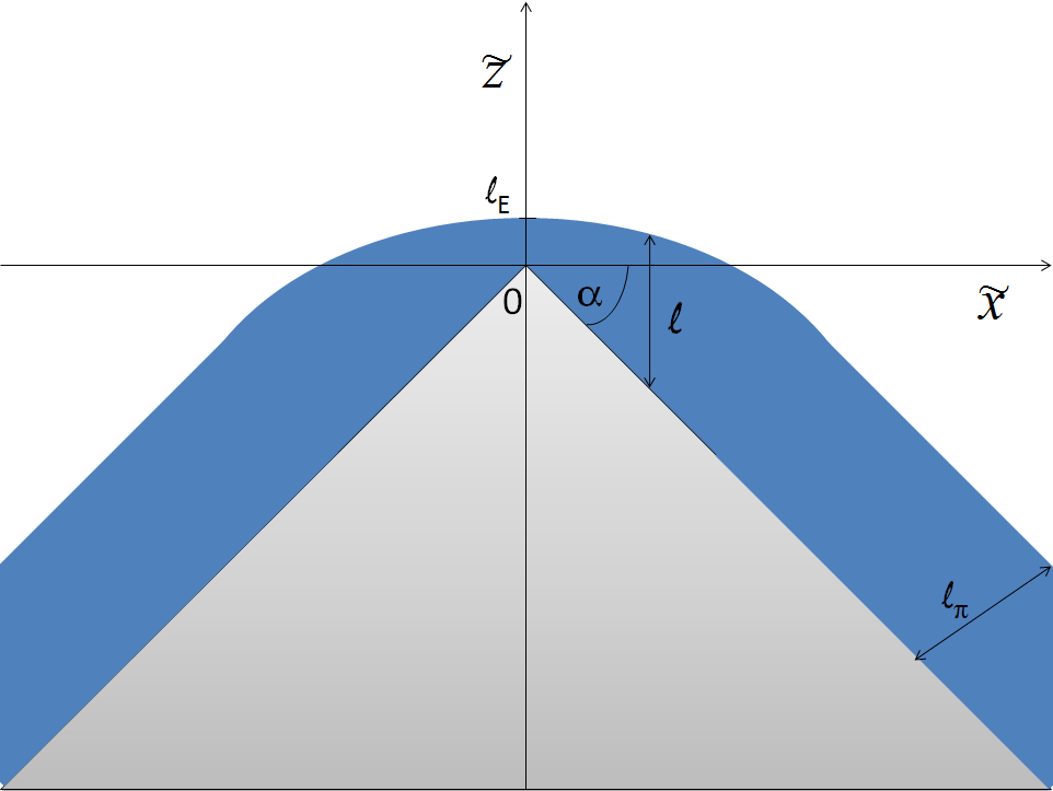
Figure 2: A sketch of the substrate model that was used by the interface Hamiltonian theory. The geometry of the substrate is identical to that of Model 1, so that the tilt angle $\alpha=\pi/4$. However, the coordinate system is now different, as depicted.

Within Model 2, the substrate remains assumed to be infinite along the $y$ axis, but the two other dimensions are a finite value $L$ as sketched in Fig. 1 (right). In this case, the substrate potential is

$$V_{2}(x,z)=\left\{\begin{array}[]{ll}\infty\,;&|x|<L/2\wedge|z|<L/2\,,\\ \tilde{V_{2}}(x,z)\,;&{\rm otherwise\,,}\end{array}\right.$$ (19)

with

$$\tilde{V_{2}}(x,z) = \rho_{w}\int_{-L/2}^{L/2}dx^{\prime}\int_{-\infty}^{\infty}dy^{\prime}\int_{-L/2}^{L/2}dz^{\prime}$$

$$\phi\left(\sqrt{(x-x^{\prime})^{2}+y^{\prime 2}+(z-z^{\prime})^{2}}\right)\,,$$

leading to

$$\tilde{V_{2}}(x,z)=-\frac{\pi}{2}\varepsilon_{w}\sigma^{6}\rho_{w}\int_{-L/2-x}^{L/2-x}dx^{\prime}\left[\Psi\left(x^{\prime},\frac{L}{2}-z\right)-\Psi\left(x^{\prime},-\frac{L}{2}-z\right)\right]\,,$$ (21)

where $\Psi(x,z)=\frac{z(3x^{2}+2z^{2}+3\sigma^{2})}{(x^{2}+\sigma^{2})^{2}(x^{2}+z^{2}+\sigma^{2})^{\frac{3}{2}}}$, which can be solved analytically.

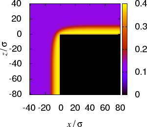
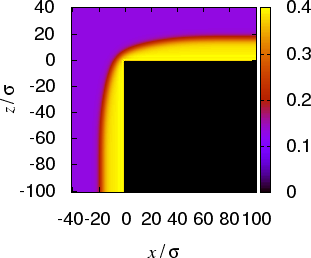
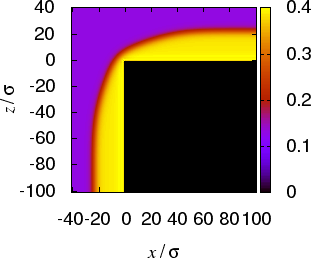
Figure 3: Density profiles $\rho(x,z)$ for a fluid at the interface between a semi-infinite rectangular substrate and a bulk vapour of temperature $k_{B}T/\varepsilon=1.35$ and undersaturation $(\rho_{v}-\rho_{b})\sigma^{3}$ (from left to right): a) $10^{-3}$, b) $10^{-4}$ and c) $2\cdot 10^{-5}$.

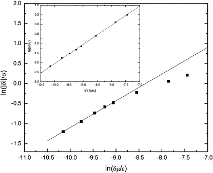
Figure 4: A log-log plot of the dependence of the film thickness above the edge relative to the saturation value, $\delta\ell=\ell_{E}-\ell_{E}^{0}$, on the chemical potential offset from the coexistence $\delta\mu$ for $k_{B}T/\varepsilon=1.35$. The symbols represent the DFT results as obtained by Model 1. The fitting line has a gradient of $3/2$, suggesting $\delta\ell\sim\delta\mu^{\frac{2}{3}}$, which is consistent with Eq. (29). In the inset, a log-log plot of the dependence of $\delta\ell^{\prime}=\delta\ell+C_{1}\delta\mu^{\frac{2}{3}}$ on $\delta\mu$ is shown. The fitting line has a gradient of $1$, which supports the linear form of the second-order correction as predicted by the effective Hamiltonian theory, cf. Eq. (29).

Using the external potentials $V_{i}(x,z)\,,i=1,2$, the Euler-Lagrange equations (10) are numerically solved for the equilibrium profile $\rho(x,z)$ on a 2D Cartesian grid with a spacing of $0.05\,\sigma$, and the corresponding integrals are performed using a Gaussian quadrature as described in Ref.  mal . To model the coupling of the system with the bulk reservoir, we impose the following boundary conditions: For Model 1, we set $\rho(L_{c},z>0)=\rho_{\pi}(z)$ and $\rho(x<0,-L_{c})=\rho_{\pi}(-x)$, where $L_{c}$ is a cut-off of the wall, and $\rho_{\pi}(z)$ is the equilibrium density profile on a corresponding planar wall. For each bulk density (chemical potential), the grand potential minimisation is performed for different values of $L_{c}$ to check any possible finite-size effect on the density distribution near the edge. For Model 2, we simply fix the density along the boundary of the system to the value of the vapour bulk density $\rho_{b}$.

III Interface Hamiltonian Theory and Finite Size Scaling

From a more phenomenological perspective, the adsorption near an edge can also be studied using the interfacial Hamiltonian model wood ; parry_apex :

$$H[\ell]=\int{\rm d}\tilde{x}\left[\frac{\gamma}{2}\left(\frac{{\rm d}f(\tilde{x})}{{\rm d}\tilde{x}}\right)^{2}+W(\ell(\tilde{x}))\right]\,.$$ (22)

The Hamiltonian is now expressed in a new Cartesian coordinate system $\{\tilde{x},\tilde{y},\tilde{z}\}$, which is related to the original system $\{x,y,z\}$ by a rotation about the $y$ axis through a tilt angle $\alpha=(\pi-\phi)/2$ (see Fig 2); thus, the height of the wall is $\tilde{z}_{w}=-\tan(\alpha)|\tilde{x}|$. Bearing in mind that for a rectangular wedge $\alpha=\pi/4$, the following analysis leaves the tilt angle unspecified. The function $f(\tilde{x})=\ell(\tilde{x})-\tan(\alpha)|\tilde{x}|$ denotes the local height of the liquid-gas interface relative to the horizontal, and $\ell(\tilde{x})$ is the local film thickness measured vertically. The first term in (22) penalises the increase of the liquid-vapour surface because of its non-planar shape, where $\gamma$ is the corresponding surface tension, while $W(\ell)$ is the planar binding potential describing the interaction of the interface and the wall. Since the translation invariance of $\ell$ along the $y$ axis is assumed, $H[l]$ denotes the Hamiltonian of the system per unit length. We notice that $W(\ell)$ can be obtained from the DFT as a coarse-grained excess (over bulk) grand potential (7) using a sharp-kink approximation to the density profile dietrich . In a mean-field approximation, the Hamiltonian (22) is simply minimised to yield the Euler-Lagrange equation

$$\gamma\ddot{\ell}(\tilde{x})=\frac{\partial W(\ell(\tilde{x}))}{\partial\ell}\,,$$ (23)

subject to the boundary conditions $\dot{\ell}(0^{+})=\tan{\alpha}$ and $\lim_{\tilde{x}\to\infty}\ell(\tilde{x})=\ell_{\pi}\sec\alpha$, where $\ell_{\pi}$ is the equilibrium film thickness on a planar wall, and $\dot{\ell}\equiv\frac{{\rm d}\ell(\tilde{x})}{{\rm d}\tilde{x}}$ (note that $\ddot{\ell}=\ddot{f}$). The Euler-Lagrange equation has a first integral, which provides an implicit equation for the height of the interface above the edge $\ell_{E}$:

$$\frac{\gamma\tan^{2}\alpha}{2}=W(\ell_{E})-W(\ell_{\pi}\sec\alpha)\,,$$ (24)

which can be solved solely from knowledge of the wetting properties of the corresponding planar wall ($\alpha=0$).

At the bulk coexistence, $\ell_{\pi}\to\infty$ for $T>T_{w}$, thus the last term in Eq. (24) vanishes. Then the height of the interface above the edge acquires a simple form (cf. Ref. parry_apex ):

$$\ell_{E}^{0}\equiv\ell_{E}(\delta\mu=0)=\sqrt{\frac{2B}{\gamma\tan^{2}\alpha}}\,,$$ (25)

where $B$ is the Hamaker constant defined by (3). Because the fluid-fluid interaction is short-ranged, the Hamaker constant can be obtained from (18):

$$W(\ell)=-\Delta\rho\int_{\ell}^{\infty}{\rm d}z\tilde{V_{\pi}}(z)=\frac{B}{\ell^{2}}+{\cal{O}}(\ell^{-4})\,,$$ (26)

with $B=\frac{\pi}{3}\varepsilon_{w}\rho_{w}\sigma_{w}^{6}\Delta\rho$.

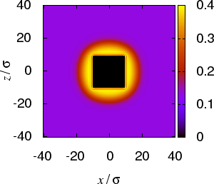
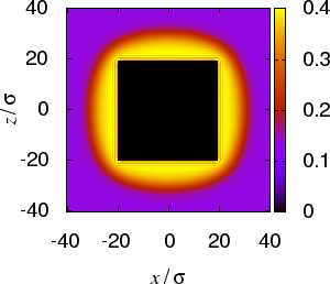
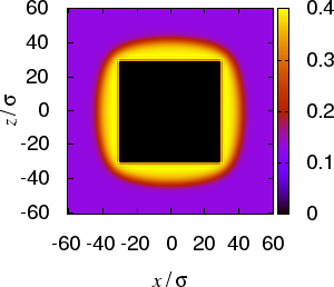
Figure 5: Examples of density profiles $\rho(x,z)$ of a fluid at the interface between a bulk saturated vapour at temperature $k_{B}T=1.35\varepsilon$ and a rectangular substrate of the size (from left to right): a) $L=20\sigma$, b) $L=40\sigma$ and c) $L=60\sigma$.

Figure 6: A log-log plot of the dependence of the meniscus height above the edge on the linear dimension of the wall of size $L$. The symbols represent the numerical DFT data corresponding to systems with saturated bulk vapour at $k_{B}T=1.35\varepsilon$. The gradient of the straight line fit is $-1.002$ compared to a predicted gradient of $-1$, see Eq. (31).

We are now concerned with the limit $\delta\mu\to 0^{+}$. Substituting $\ell_{E}=\ell_{E}^{0}+\delta\ell$ into Eq. (24) and introducing the abbreviation $A=\gamma\tan^{2}(\alpha)/2$, one obtains

$$A=\delta\mu\Delta\rho\ell_{E}^{0}+\frac{B}{(\ell_{E}^{0})^{2}}-\frac{2B}{(\ell_{E}^{0})^{3}}\delta\ell-W(\ell_{\pi}\sec\alpha)+H.O.T.$$ (27)

Using (6) and (25), it follows that

$$\delta\ell\sim-C_{1}\delta\mu^{2-\alpha_{s}^{co}}+C_{2}\delta\mu\,,$$ (28)

as $\delta\mu\to 0$ and $C_{1},C_{2}>0$. Finally, upon substituting $\alpha_{s}^{co}$ from Eq. (6), the exponent $\beta_{E}^{co}$ defined in Eq. (1) becomes $\beta_{E}^{co}=p/(p+1)$. More specifically, for van der Waals forces ($p=2$):

$$\delta\ell=-C_{1}\delta\mu^{\frac{2}{3}}+C_{2}\delta\mu+{\cal{O}}(\delta\mu^{\frac{4}{3}})\,.$$ (29)

In terms of Model 2, the asymptotic result (28) must be modified due to the finiteness of the linear dimension of the wall $L$ competing with the correlation length $\xi_{\parallel}$. Therefore, recalling the finite-size scaling arguments (see, e.g., [32]), the result of equation (28) valid for $L\to\infty$ becomes rescaled with a scaling function $F$:

$$\delta\ell_{E}(L) \propto \delta\mu^{2-\alpha_{s}^{co}}F\left(\frac{L}{\xi_{||}}\right)+{\cal O}\left(\delta\mu F\left(\frac{L}{\xi_{||}}\right)\right)$$

$$\propto \delta\mu^{2-\alpha_{s}^{co}}F(L\delta\mu^{\nu_{||}^{co}})+{\cal O}\left(\delta\mu F(L\delta\mu^{\nu_{||}^{co}})\right)\,,$$

which must remain finite as $\delta\mu\to 0$. Therefore,

$$\delta\ell_{E}(L) \propto L^{\frac{\alpha_{s}^{co}-2}{\nu_{||}^{co}}}+{\cal O}\left(L^{-\frac{1}{\nu_{||}^{co}}}\right)$$ (31)

$$\propto L^{-1}+{\cal{O}}(L^{-\frac{3}{2}})$$

where the values $\alpha_{s}^{co}=4/3$ and $\nu_{||}^{\rm co}=2/3$ were substituted in the final expression.

IV Numerical Results

We now examine the functional forms of (29) and (31) by a comparison with the numerical solution of the microscopic DFT, as described in section 2. We adopt $\sigma$ and $\varepsilon$ as the length and energy units, respectively, and we fix the strength of the wall potential to $\varepsilon_{w}=0.4\varepsilon$, for which the wetting temperature is $k_{B}T_{w}/\varepsilon=1.25$, which is sufficiently below the bulk critical temperature $k_{B}T_{c}/\varepsilon=1.41$. We begin with the case of a semi-infinite wall as described by Model 1. For a given value of $\delta\mu$, we first determine the equilibrium density profile $\rho_{\pi}(z)$ for a corresponding system with a planar wall, which constitutes a boundary condition for the system with a single edge. For the sake of numerical consistency, the profile $\rho_{\pi}(z)$, albeit varying only in one dimension, is determined on the same two-dimensional grid as used for the edge. This also provides a good test of our numerics, since the difference between the planar density profile that is constructed from a 2D calculation proved not to appreciably differ from that obtained from a standard 1D treatment. Moreover, the numerical accuracy of the full 2D DFT code, described in details in Ref. mal , was verified by comparison of the DFT results with the exact pressure sum-rule mal_parry_wedge . Then we set the boundary conditions such that $\rho(L_{c},z>0)=\rho_{\pi}(z)$ and $\rho(x<0,-L_{c})=\rho_{\pi}(-x)$, where the value of the wall cut-off $L_{c}$ ranges from $L_{c}=40\sigma$ to $L_{c}=100\sigma$ to verify that the system size does not affect $\ell_{E}$.

The representative samples of the equilibrium density profiles are shown in Fig. 3. The height of the fluid interface above the edge is defined as follows:

$$\ell_{E}=\frac{\sqrt{2}}{\Delta\rho}\int_{-\infty}^{0}{\rm d}x\left(\rho(x,-x)-\rho_{b}\right)\,,$$ (32)

where $\rho_{b}$ is the density of the gas reservoir. Eq. (32) allows us to compare the DFT results with the prediction based on the interface Hamiltonian theory as given by (29). The comparison that is displayed in Fig. 4 reveals a consistency between the two approaches and verifies the values of the exponents of the two first terms in Eq. (29).

Next, we consider Model 2 and examine the validity of the expansion (31). In the DFT, the density at the boundary of the system is fixed to the value of the bulk density of the saturated vapour, $\rho_{b}=\rho_{v}$, and the linear dimension of the box size is chosen from a range between $80\sigma$ and $120\sigma$. Varying the wall size $L$, we find the equilibrium state of each system as shown in Fig. 5. In Fig. 6, we display a log-log plot of the height of the interface above the edge $\ell_{E}$ versus the wall size $L$. The values of $\ell_{E}$ are again determined using formula (32), where the upper limit is $-L_{c}/2$. The fitted line shows a good agreement between the DFT and the analytic expression (31), and for the region of $L>20\sigma$, the first-order term in Eq. (31) appears to dominate. The consistency between the gradient of the fitted line and the predicted value $-1$ is within an error of $0.2\%$.

V Conclusion

In this work, we used an interfacial Hamiltonian theory and a fundamental-measure DFT to study the fluid adsorption near a rectangular edge of a substrate interacting with the fluid via van der Waals forces. When the two-phase bulk coexistence is approached from below at a fixed temperature, i.e., the deviation of the chemical potential from the coexistence $\delta\mu=\mu_{\rm s}-\mu\to 0^{+}$, macroscopically thick films are formed at the wall far away from the edge. Because these asymptotic interfaces must eventually merge to form a meniscus, the local height of the interface above the edge $\ell_{E}$ remains finite and indeed rather small even at the bulk coexistence. In this paper, we have shown that for an infinitely long substrate, $\ell_{E}(\delta\mu)$ approaches the coexistence value according to $\delta\ell=\ell_{E}(0)-\ell_{E}(\delta\mu)\sim\delta\mu^{\beta_{E}^{co}}$ as $\delta\mu\to 0^{+}$. The exponent depends on the range of the molecular interaction, such that $\beta_{E}^{co}=p/(p+1)$, where $p$ defines the asymptotic decay of the binding potential $W(\ell)\sim\ell^{-p}$. The second-order correction to $\delta\ell$ is linear in $\delta\mu$ regardless of the molecular interaction. Both findings were verified by the DFT numerical calculations. We also showed that if the substrate is of finite size $L$, the previous result corresponds to the scaling of $\ell_{E}$ as $\ell_{E}-\ell_{E}(L)\propto L^{-1}+{\cal{O}}(L^{-\frac{3}{2}})$, as also confirmed by the DFT. We conclude with two remarks about the generality of these findings. First, throughout this study, the substrate geometry was maintained fixed such that the substrate edge was rectangular. This geometry was selected because the model of a right-angle edge appears important considering its connection with other fundamental substrate models as discussed in the introduction. Technically, the external potential for the rectangular geometry remains rather simple, which facilitates the numerics in the DFT, and the application of the finite-size arguments is straightforward. Nevertheless, we believe that the result given by Eq. (1) is valid for an arbitrary internal angle, since the value of $\phi$ was not assumed in the derivation of (1). Second, because the edge geometry does not induce any new divergence compared to a planar wall, the upper critical dimension $d_{u}$ corresponding to complete wetting must be identical for the two substrates. Since $d_{u}<3$ for a finite $p$ for a planar wall lipowsky , our mean-field results remain unaffected by the capillary-wave fluctuations.

- (1) S. Dietrich, in New Approaches to Problems in Liquid State Theory, edited by C. Caccamo, J. P. Hansen, and G. Stell (Kluwer, Dordrecht, 1999).
- (2) D. Bonn, J. Eggers, J. Indekeu, J. Meunier, and E. Rolley, Rev. Mod. Phys. 81, 739 (2009).
- (3) W. F. Saam, J. Low Temp. Phys. 157, 77 (2009).
- (4) E. H. Hauge, Phys. Rev. A 46, 4994 (1992).
- (5) K. Rejmer, S. Dietrich, and M. Napirkówski, Phys. Rev. E 60, 4027 (1999).
- (6) A. O. Parry, C. Rascón, and A. J. Wood, Phys. Rev. Lett. 83, 5535 (1999).
- (7) C. Rascón and A. O. Parry, Nature 407, 986 (2000).
- (8) N. M. Silvestre, Z. Eskandari, P. Patr cio, J. M. Romero-Enrique, and M. M. Telo Da Gama, Phys. Rev. E 86, 011703 (2012).
- (9) C. Rascón C and A. O. Parry, Phys. Rev. Lett. 94, 096103 (2005).
- (10) M. Tasinkevych and S. Dietrich, Phys. Rev, Lett. 97, 106102 (2006).
- (11) G. M. Whitesides and A. D. Stroock, Phys. Today 54, 42 (2001).
- (12) D. Quéré, Annu. Rev. Mater. Res. 38, 71 (2008).
- (13) M. Rauscher and S. Dietrich, Annu. Rev. Mater. Res. 38, 143 (2008).
- (14) R. Fürstner, W. Barthlott, C. Neinhuis and P. Walzel, Langmuir 21, 956 (2005).
- (15) S. Minko, Polymer Rev. 46 , 397 (2006).
- (16) R. F. Service, Science 282 , 399 (1998).
- (17) M. C. Stewart and R. Evans, Phys Rev. E 71, 011602 (2005).
- (18) A. Nold, A, Malijevský, and S. Kalliadasis, Phys. Rev. E 84, 021603 (2011).
- (19) L Bruschi, A. Carlin and G. Mistura, Phys. Rev. Lett 89, 166101 (2002).
- (20) L. Bruschi, G. Fois, G. Mistura, M. Tormen, V. Garbin, E. di Fabrizio, A Gerardino and M. Natali, J. Chem. Phys 125, 144709 (2006).
- (21) M. Tasinkevych and S. Dietrich, Eur. Phys. J. E 23, 117 (2007).
- (22) T. Hofmann, M. Tasinkevych, A. Checco, E. Dobisz, S. Dietrich, and B. M. Ocko, Phys. Rev. Lett. 104, 106102 (2010).
- (23) A. Checco, B. M. Ocko, M. Tasinkevych, and S. Dietrich, Phys. Rev. Lett. 109, 166101 (2012).
- (24) A. Malijevský, J. Phys.: Condens Matter 25, 445006 (2013).
- (25) C. Rascón, A. O. Parry, and A. Sartori, Phys. Rev. E 59, 5697 (1999).
- (26) A. O. Parry, M. J. Greenall, and J. M. Romero-Enrique, Phys. Rev. Lett. 90, 046101 (2003).
- (27) S. Dietrich, in Phase Transitions and Critical Phenomena, edited by C. Domb and J. L. Lebowitz (Academic, New York, 1988), Vol. 12.
- (28) R. Lipowsky, Phys. Rev. Lett. 52, 1429 (1984).
- (29) R. Evans, Adv. Phys. 28, 143 (1979).
- (30) Y. Rosenfeld, Phys. Rev. Lett 63, 980 (1989).
- (31) R. Roth, J. Phys.: Condens. Matter 22, 063102 (2010).
- (32) M. E. Fisher and H. Nakanishi, J. Chem. Phys 75, 5857 (1981).
- (33) A. Malijevský and A. O. Parry, J. Phys.: Condens. Matter 25, 305005 (2013).