Stripe formation instability in crossing traffic flows

Abstract

At the intersection of two unidirectional traffic flows a stripe formation instability is known to occur. In this paper we consider coupled time evolution equations for the densities of the two flows in their intersection area. We show analytically how the instability arises from the randomness of the traffic entering the area. The Green function of the linearized equations is shown to form a Gaussian wave packet whose oscillations correspond to the stripes. Explicit formulas are obtained for various characteristic quantities in terms of the traffic density and comparison is made with the much simpler calculation on a torus and with numerical solution of the evolution equations.

1 Introduction

In traffic dynamics, crossing flows, whether of pedestrians or of vehicles, have attracted a certain amount of attention in recent years. The crossing of two single lanes was studied, for example, in Refs. [1, 2, 3, 4, 5]. Here we will turn our interest towards wider lanes, that have been the object of experimental studies on pedestrians [6, 7, 8, 9, 10] and for which realistic models have been designed [11, 12]. Monte Carlo studies of simpler cellular automaton models of such intersecting flows were carried out by several groups [13, 14, 15, 16, 17, 18, 19, 20, 21, 22, 23] including ourselves [24, 25, 26, 27]. In most of the studies cited a vehicle or a pedestrian, as the case may be, is represented by a hard core particle on a lattice site. It is known from simulations [13, 11, 12, 21, 28] and from experiments [6, 7, 29, 8, 9, 30] that when two unidirectional flows cross, whether perpendicularly or at an angle, there arises a stripe formation instability. In the case of perpendicular flows, in the square region where the flows intersect the two kinds of particles show a pattern of alternating stripes approximately or exactly perpendicular to the $(1,1)$ direction, as shown in Fig. 1. It is the purpose of this work better to understand this stripe formation instability in perpendicularly crossing flows.

The analytic approach to this problem, and in fact to almost any question concerning crossing particle flows, is very hard: these are strongly interacting many-particle systems. As a simplification we introduce two continuous fields $\rho^{\cal E}_{i,j}(t)$ and $\rho^{\cal N}_{i,j}(t)$ (${\cal E}$ for eastbound and ${\cal N}$ for northbound) representing the densities of the two species at times $t=0,1,2,\ldots$ on the lattice sites $i,j=1,2,\ldots,M$ that represent the intersection square. Then, largely independently of the precise microscopic rules of motion of the particles, one postulates the time evolution equations

$$\rho^{\cal E}_{i,j}(t+1) = (1-\rho^{\cal N}_{i,j}(t))\rho^{\cal E}_{i-1,j}(t)+\rho^{\cal N}_{i+1,j}(t)\rho^{\cal E}_{i,j}(t),$$

$$\rho^{\cal N}_{i,j}(t+1) = (1-\rho^{\cal E}_{i,j}(t))\rho^{\cal N}_{i,j-1}(t)+\rho^{\cal E}_{i,j+1}(t)\rho^{\cal N}_{i,j}(t),$$ (1)

whose boundary conditions we will discuss shortly. These equations are believed [24, 25] to be representative of the class of unidirectional deterministic particle dynamics at sufficiently low density, irrespective of the exact details of the evolution at the particle level. In the absence of the nonlinear terms all particles would simply cross the square at unit velocity without any impediment. The terms in (1) that are quadratic in the densities express that an ${\cal E}$ particle that tries to hop forward will be blocked if there is a ${\cal N}$ particle on its target site, and the other way around. Blockings between same-type particles are expected to correspond to higher order effects in the density [25] and are neglected in this description.

Eqs. (1) have to be supplied with initial and boundary conditions. Following the example of the BML model [13] several authors have studied crossing flows with periodic boundary conditions. If one adopts periodic boundary conditions (PBC) equations (1) are translationally invariant in both the $i$ and the $j$ direction and therefore allow for a uniform stationary state in which $\rho^{\cal E}_{i,j}(t)=\rho^{\cal N}_{i,j}(t)=\rho$ for all $i,j$, with a value of $\rho$ determined by the initial condition. However, a linear stability analysis shows that this stationary state is unstable to random perturbations of the initial condition (Ref. [25], section 4). One of the few analytic results in this field is an expression for the wavelength and the growth rate of the most unstable mode as a function of the density.

The true problem of crossing flows, however, has open boundary conditions (OBC) and is driven by a random inflow of particles at its western and southern boundaries. Whereas the calculation with periodic boundary conditions does make the observed instability plausible, the question nevertheless remains whether random boundary conditions, rather than random initial conditions, lead to the same instability. In this paper we address this problem. We do so again by linearizing Eqs. (1), but now under random boundary conditions at the two entrance boundaries. Specifically, we will use Eqs. (1) for $i,j=1,2,\ldots,M$ with the stipulation that

$$\rho^{\cal E}_{0,j}(t)=\rho+\eta^{\cal E}_{j}(t),\qquad j=1,\ldots,M,$$

$$\rho^{\cal N}_{i,0}(t)=\rho+\eta^{\cal N}_{i}(t),\qquad i=1,\ldots,M,$$ (2)

in which $\eta^{\cal E}_{j}(t)$ and $\eta^{\cal N}_{i}(t)$ are noise terms of zero mean that express that the particles enter randomly; these terms may be associated with the ‘entrance sites’ in Fig. 1. On the exit boundaries we make the most convenient choice $\rho^{\cal E}_{i,M+1}(t)=\rho^{\cal N}_{M+1,j}(t)=\rho$ for all $i,j=1,\ldots,M$, keeping in mind that this choice has very little influence on the physical properties of the system.

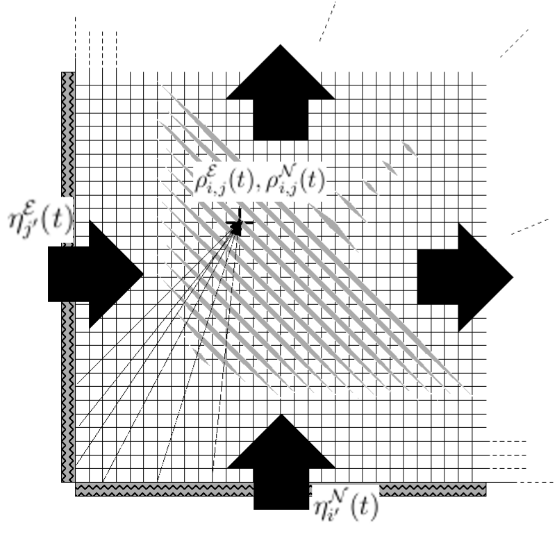
Figure 1: Schematic representation of the square region where the crossing flows interact. The boundary noise $\eta^{\cal E}_{j^{\prime}}(t)$ and $\eta^{\cal N}_{i^{\prime}}(t)$ is applied at the west and south boundaries of an $M\times M$ square grid. The perturbations of the density fields $\rho^{\cal E}_{i,j}(t)$ and $\rho^{\cal N}_{i,j}(t)$ propagate eastward and northward according to Eqs. (1), and exit the system at the east and north boundaries. The stripe instability is shown.

After an analysis of considerable complexity we find that the random boundary conditions (1), too, lead to a stripe formation instability. We compare the expression for its $\rho$ dependent growth rate and maximally unstable wavelength with those found under periodic boundary conditions in Refs. [24, 25] and find – which was far from obvious a priori – that they are identical. The stripe formation instability therefore appears to be an intrinsic property of the equations.

Our work furnishes, moreover, a new look onto the problem. We find that an instantaneous and localized perturbation applied at a boundary site and superposed on a uniform background of density $\rho$ propagates inward along a diagonal at a group velocity $\overline{v}_{\rm g}$ that we are able to determine as a function of the background density $\rho$. This propagating pulse widens diffusively, hence acquiring a Gaussian envelope. We are able to calculate its widths along and perpendicularly to the direction of propagation. In addition, the propagating pulse shows oscillations that we fully characterize analytically, thereby demonstrating that stripe formation indeed occurs. The structure and dimensions of the pulse are shown schematically in figure 2.

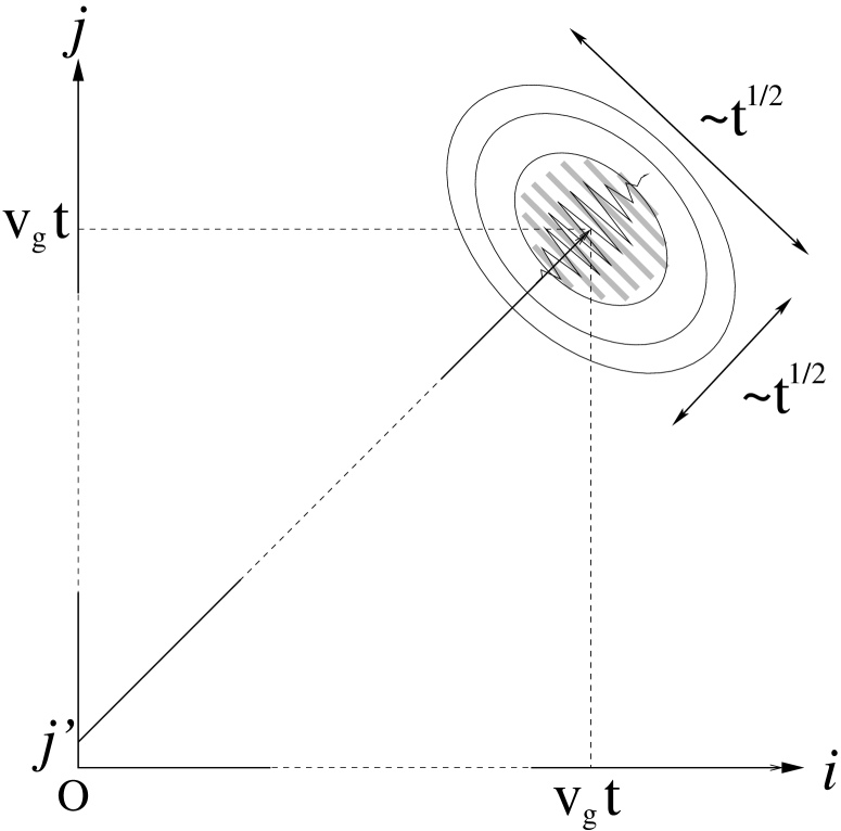
Figure 2: Typical shape of the Green functions. Here the ${\cal E}$ density has been perturbed on the boundary site $(1,j^{\prime})$ at time $t^{\prime}=0$. After a long enough time $t$ the Green function consists in a Gaussian wavepacket centered at $(i,j)=(v_{\rm g}t,v_{\rm g}t)$, where the velocity $v_{\rm g}$ is determined in Eq. (63). The represented wave packet is wider in the direction perpendicular to the diagonal in accordance with equations (67) and (76).

This paper is organized as follows. In section 2 we linearize Eqs. (1) and obtain a system governed by a $2M^{2}\times 2M^{2}$ time evolution matrix. Green functions are defined for each of the four $M^{2}\times M^{2}$ subblocks. The equations are solved in terms of generating functions in subsection 2.1. This solution is partially formal and involves $M^{2}\times M^{2}$ matrices $\mathbf{E}$ and $\mathbf{F}$. These matrices are made explicit in subsection 2.2, where we also carry out the required diagonalization of $\mathbf{F}$. In subsection 2.3 we combine the preceding results and obtain fully explicit exact expressions for the four Green functions for finite $M$, which take the form of an inverse Fourier-Laplace transform. In section 3 we perform an asymptotic expansion valid for large times and distances and calculate the properties of the propagating wave packet. The expansion starts with finding, in subsection 3.1, the poles of the Green function in the plane of the variable $z$ conjugate to time. In subsection 3.2 we select the pole expected to dominate in the large time limit. The asymptotic analysis then becomes a saddle-point calculation in the planes of the Fourier variables. The general structure of this calculation is discussed in subsection 3.3. The wave packet is studied explicitly along the diagonal in subsection 3.4 and in the vicinity of the diagonal in subsection 3.5. Section 4 summarizes the results and concludes the paper.

2 Linearized equations

In this section we will study the linearized version of the time evolution equations (1). We write $\rho^{\cal X}_{i,j}(t)=\rho+p^{\cal X}_{i,j}(t)$ for all $1\leq i,j\leq M$, where ${\cal X}={\cal E},{\cal N}$, the $p^{\cal X}_{i,j}(t)$ are small, and $\rho$ is the average of the entrance site densities defined in Eq. (1). The linearization of Eqs. (1) reads

$$p^{\cal E}_{i,j}(t+1) = (1-\rho)p^{\cal E}_{i-1,j}(t)+\rho p^{\cal E}_{i,j}(t)-\rho p^{\cal N}_{i,j}(t)+\rho p^{\cal N}_{i+1,j}(t),$$

$$p^{\cal N}_{i,j}(t+1) = (1-\rho)p^{\cal N}_{i,j-1}(t)+\rho p^{\cal N}_{i,j}(t)-\rho p^{\cal E}_{i,j}(t)+\rho p^{\cal E}_{i,j+1}(t)$$ (3)

for $1\leq i,j\leq M$ and $t=0,1,2,\ldots$ for all $M\geq 1$. The entrance boundary conditions (1) become

$$p^{\cal E}_{0,j}(t)=\eta^{\cal E}_{j}(t),\qquad j=1,\ldots,M,$$

$$p^{\cal N}_{i,0}(t)=\eta^{\cal N}_{i}(t),\qquad i=1,\ldots,M.$$ (4)

and the exit boundary conditions are

$$p^{\cal E}_{i,M+1}(t)=p^{\cal N}_{M+1,j}(t)=0\qquad i,j=1,\ldots,M.$$ (5)

We will take the system at the initial time $t=0$ in a state of uniform density $\rho$, that is,

$$p^{\cal X}_{i,j}(0)=0,\qquad{\cal X}={\cal E},{\cal N}.$$ (6)

Eqs. (2), (5), and (6) are homogeneous in the $p^{\cal X}_{i,j}(t)$ so that the whole system (2)-(6) would have only the zero solution if the entrance noises $\eta^{\cal E}_{j}(t)$ and $\eta^{\cal N}_{i}(t)$ both vanished. The problem (2)-(6) is linear, and its solution may therefore be written as a convolution of the time dependent boundary noise with an appropriate Green function. Given a unit perturbation applied on a boundary site $(i^{\prime},0)$ or $(0,j^{\prime})$ at some time $t^{\prime}$ to one of the two entering fluxes, the Green function tells us the effect on the densities at arbitrary later times $t>t^{\prime}$ at arbitrary lattice sites $(i,j)$.

2.1 Solution in terms of generating functions

Let ${p^{\cal E}}(t)$ stand for the $M^{2}$-component vector containing all values of the fields $p^{\cal E}_{i,j}(t)$, and similarly ${p^{\cal N}}(t)$ for the vector of the $p^{\cal N}_{i,j}(t)$. Equations (2)-(5) may be written vectorially with the aid of two $M\times M$ matrices $\mathbf{A}$ and $\mathbf{B}$ defined by

$$\mathbf{A}_{i;i^{\prime}}\equiv(1-\rho)\delta_{i;i^{\prime}+1}+\rho\delta_{i;i^{\prime}},$$ (7)

$$\mathbf{B}_{i;i^{\prime}}\equiv-\rho\delta_{i;i^{\prime}}+\rho\delta_{i;i^{\prime}-1},$$ (8)

where $\delta_{i;i^{\prime}}=1$ if $i=i^{\prime}$ and $0$ otherwise. Letting $\mathbf{I}$ stand for the $M\times M$ identity matrix we now define four $M^{2}\times M^{2}$ matrices that act on the tensor product space between columns $i$ and rows $j$,

$$\mathbf{M^{{\cal E}{\cal E}}} \equiv \mathbf{A}\otimes\mathbf{I},$$

$$\mathbf{M^{{\cal E}{\cal N}}} \equiv \mathbf{B}\otimes\mathbf{I},$$

$$\mathbf{M^{{\cal N}{\cal E}}} \equiv \mathbf{I}\otimes\mathbf{B},$$ (9)

$$\mathbf{M^{{\cal N}{\cal N}}} \equiv \mathbf{I}\otimes\mathbf{A},$$

that is, componentwise, $[\mathbf{M^{{\cal E}{\cal E}}}]_{i,j;i^{\prime},j^{\prime}}=\mathbf{A}_{i;i^{\prime}}\mathbf{I}_{j;j^{\prime}}$, etc. Upon setting $p(t)\equiv{{p^{\cal E}}(t)\choose{p^{\cal N}}(t)}$ and $\eta(t)\equiv{\mathbf{\eta^{\cal E}}(t)\choose\mathbf{\eta^{\cal N}}(t)}$ we may cast the system (2)-(5) of linearized equations in the form

$${p}(t+1)=\mathbf{M}{p}(t)+(1-\rho)\mathbf{\eta}(t),$$ (10)

in which

$$\mathbf{M}\equiv\left(\begin{array}[]{cc}\mathbf{M^{{\cal E}{\cal E}}}&\mathbf{M^{{\cal E}{\cal N}}}\\ \mathbf{M^{{\cal N}{\cal E}}}&\mathbf{M^{{\cal N}{\cal N}}}\end{array}\right),$$ (11)

and with the noise vectors defined as $(\mathbf{\eta^{\cal E}}(t))_{ij}=\delta_{i;1}\eta^{\cal E}_{j}(t)$ and $(\mathbf{\eta^{\cal N}}(t))_{ij}=\eta^{\cal N}_{i}(t)\delta_{j;1}$.

This linear equation may be solved by generating function methods. We define the generating function (or Laplace transform) of any $X_{t}$ by $\hat{X}(z)\equiv\sum_{t=0}^{\infty}z^{t}X_{t}$, where $z$ is a complex number within the radius of convergence of the sum. This transformation is inverted by integrating in the complex plane $X_{t}=(2\pi{\mathrm{i}})^{-1}\oint_{\Gamma_{0}}\mathrm{d}z\,z^{-t-1}\hat{X}(z)$, where $\Gamma_{0}$ runs counterclockwise around the origin. Applying this transformation to Eq. (10) with initial condition (6) gives

$$z^{-1}{\hat{p}}=\mathbf{M}{\hat{p}}+(1-\rho)\mathbf{\hat{\eta}},$$ (12)

where we omitted the argument $z$ of ${\hat{p}}$ and $\mathbf{\hat{\eta}}$. After a little algebra one obtains

$${\hat{p}^{\cal E}} = (1-\rho)(\mathbf{I}\otimes\mathbf{I}-\mathbf{F}\otimes\mathbf{F})^{-1}\bigg{[}(\mathbf{E}\otimes\mathbf{I})z\mathbf{\hat{\eta}^{\cal E}}+(\mathbf{F}\otimes\mathbf{E})z\mathbf{\hat{\eta}^{\cal N}}\bigg{]},$$

$${\hat{p}^{\cal N}} = (1-\rho)(\mathbf{I}\otimes\mathbf{I}-\mathbf{F}\otimes\mathbf{F})^{-1}\bigg{[}(\mathbf{I}\otimes\mathbf{E})z\mathbf{\hat{\eta}^{\cal N}}+(\mathbf{E}\otimes\mathbf{F})z\mathbf{\hat{\eta}^{\cal E}}\bigg{]}.$$ (13)

where

$$\mathbf{E}(z)\equiv(\mathbf{I}-z\mathbf{A})^{-1},\qquad\mathbf{F}(z)\equiv(\mathbf{I}-z\mathbf{A})^{-1}z\mathbf{B},$$ (14)

and the various inverse matrices exist for almost all values of $z$.

We define the Green functions $G^{{\cal X}{\cal Y}}$ by the convolutions

$$p^{\cal E}_{i,j}(t) = \sum_{t^{\prime}=0}^{t-1}\bigg{[}\sum_{j^{\prime}=1}^{M}G^{{\cal E}{\cal E}}_{i,j;j^{\prime}}(t-t^{\prime})\eta^{\cal E}_{j^{\prime}}(t^{\prime})+\sum_{i^{\prime}=1}^{M}G^{{\cal E}{\cal N}}_{i,j;i^{\prime}}(t-t^{\prime})\eta^{\cal N}_{i^{\prime}}(t^{\prime})\bigg{]},$$

$$p^{\cal N}_{i,j}(t) = \sum_{t^{\prime}=0}^{t-1}\bigg{[}\sum_{i^{\prime}=1}^{M}G^{{\cal N}{\cal N}}_{i,j;i^{\prime}}(t-t^{\prime})\eta^{\cal N}_{i^{\prime}}(t^{\prime})+\sum_{j^{\prime}=1}^{M}G^{{\cal N}{\cal E}}_{i,j;j^{\prime}}(t-t^{\prime})\eta^{\cal E}_{j^{\prime}}(t^{\prime})\bigg{]}.$$ (15)

The generating function may then be inverted to give the following expressions for the Green functions in terms of the matrices $\mathbf{E}$ and $\mathbf{F}$,

$$G^{{\cal E}{\cal E}}_{i,j;j^{\prime}}(t-t^{\prime}) = \frac{1-\rho}{2\pi{\mathrm{i}}}\oint_{\Gamma_{0}}\frac{\mathrm{d}z}{z^{t-t^{\prime}}}\big{[}(\mathbf{I}\otimes\mathbf{I}-\mathbf{F}\otimes\mathbf{F})^{-1}(\mathbf{E}\otimes\mathbf{I})\big{]}_{i,j;1,j^{\prime}}\,,$$

$$G^{{\cal E}{\cal N}}_{i,j;i^{\prime}}(t-t^{\prime}) = \frac{1-\rho}{2\pi{\mathrm{i}}}\oint_{\Gamma_{0}}\frac{\mathrm{d}z}{z^{t-t^{\prime}}}\big{[}(\mathbf{I}\otimes\mathbf{I}-\mathbf{F}\otimes\mathbf{F})^{-1}(\mathbf{F}\otimes\mathbf{E})\big{]}_{i,j;i^{\prime},1}\,.$$ (16)

Symmetric formulas for $G^{{\cal N}{\cal N}}_{i,j;i^{\prime}}(t-t^{\prime})$ and $G^{{\cal N}{\cal E}}_{i,j;j^{\prime}}(t-t^{\prime})$ are obtained by inversion of the column and row indices. With these expressions we have succeeded in disentangling the four $M^{2}\times M^{2}$ blocks in equation (12). They remain formal within each block until we are able to explicitize the integrands in Eqs. (2.1). This is our next task.

In order to evaluate $(\mathbf{I}\otimes\mathbf{I}-\mathbf{F}\otimes\mathbf{F})^{-1}$ we need to diagonalize $\mathbf{F}$. This will be done in detail in subsection 2.2, where we show that $\mathbf{F}$ has full biorthonormal sets of right and left eigenvectors, $\{\phi^{\lambda}\}$ and $\{\psi^{\lambda}\}$, respectively, associated with a set of eigenvalues $\{\lambda\}$. We may therefore write $\mathbf{F}=\sum_{\lambda}\psi^{\lambda}\lambda\phi^{\lambda}$ where $\sum_{\lambda}$ ranges over the whole spectrum of $\mathbf{F}$. The eigenvectors satisfy $\mathbf{F}\psi^{\lambda}=\lambda\psi^{\lambda}$ and $\phi^{\lambda}\mathbf{F}=\lambda\phi^{\lambda}$, as well as $\phi^{\lambda}\cdot\psi^{\mu}\equiv\sum_{i=1}^{M}\phi^{\lambda}_{i}\psi^{\mu}_{i}=\delta_{\lambda,\mu}$. Using the diagonal form of $\mathbf{F}$ we finally get

$$\big{[}(\mathbf{I}\otimes\mathbf{I}-\mathbf{F}\otimes\mathbf{F})^{-1}(\mathbf{E}\otimes\mathbf{I})\big{]}_{i,j;i^{\prime},j^{\prime}}=\sum_{\lambda,\mu}\frac{\psi^{\lambda}_{i}\psi^{\mu}_{j}\phi^{\mu}_{j^{\prime}}}{1-\lambda\mu}\sum_{i^{\prime\prime}=1}^{M}\phi^{\lambda}_{i^{\prime\prime}}\mathbf{E}_{i^{\prime\prime};i^{\prime}},$$ (17)

$$\big{[}(\mathbf{I}\otimes\mathbf{I}-\mathbf{F}\otimes\mathbf{F})^{-1}(\mathbf{F}\otimes\mathbf{E})\big{]}_{i,j;i^{\prime},j^{\prime}}=\sum_{\lambda,\mu}\lambda\frac{\psi^{\lambda}_{i}\psi^{\mu}_{j}\phi^{\lambda}_{i^{\prime}}}{1-\lambda\mu}\sum_{j^{\prime\prime}=1}^{M}\phi^{\mu}_{j^{\prime\prime}}\mathbf{E}_{j^{\prime\prime};j^{\prime}}.$$ (18)

The important achievement here is that with Eqs. (17) and (18) we have come as near as is possible to decoupling the motion in the two orthogonal directions: the right hand members of each of these equations would factorize into an $i$ and a $j$ dependent part if it were not for the factor $(1-\lambda\mu)^{-1}$. This factor is a very succinct representation in reciprocal space of the interaction between the two flows.

2.2 Diagonalizing  $\mathbf{F}$

In order to prepare for diagonalizing $\mathbf{F}$ we will first find the explicit expressions of its matrix elements $\mathbf{F}_{i;i^{\prime}}$. From Eq. (7) it follows that $[\mathbf{A}^{n}]_{i;i^{\prime}}=\sum_{k=0}^{n}{n\choose k}\rho^{n-k}(1-\rho)^{k}\delta_{i;i^{\prime}+k}$ for $i,i^{\prime}=1,\ldots,M$. We define $\zeta\equiv\frac{(1-\rho)z}{1-\rho z}$, which has the inverse $z=\frac{\zeta}{(1-\rho)+\rho\zeta}$. For the matrix $\mathbf{E}$ we get

$$\mathbf{E}_{i;i^{\prime}} = \sum_{p=0}^{\infty}z^{p}[\mathbf{A}^{p}]_{i;i^{\prime}}$$ (19)

$$= \Theta(i\geq i^{\prime})\frac{1}{1-z\rho}\zeta^{i-i^{\prime}}$$

with $\Theta(a)=1$ if assertion $a$ is true and $0$ otherwise. Eq. (19) is valid when the sums converge, i.e. for $|z|<\rho^{-1}$. From equations (14) and (19) we find

$$\mathbf{F}_{i;i^{\prime}} = [\mathbf{E}z\mathbf{B}]_{i;i^{\prime}}$$ (20)

$$= (\zeta\Theta(2\leq i^{\prime}\leq i+1)-\Theta(1\leq i^{\prime}\leq i))\frac{z\rho}{1-z\rho}\zeta^{i-i^{\prime}},$$

which is the desired explicit expression.

We write $\mathbf{F}_{i;i^{\prime}}=\frac{z\rho}{1-z\rho}\zeta^{i-i^{\prime}}\mathbf{\tilde{F}}_{i;i^{\prime}}$, where

$$\mathbf{\tilde{F}}=\left(\begin{array}[]{cccc}-1&\zeta&0&\ldots\\ -1&-1+\zeta&\zeta&\ddots\\ -1&-1+\zeta&-1+\zeta&\ddots\\ \vdots&\vdots&\vdots&\ddots\end{array}\right).$$

The right and left eigenvectors and the eigenvalues of $\mathbf{\tilde{F}}$ will be denoted by $\mathbf{\tilde{\psi}^{\lambda}}$, $\mathbf{\tilde{\phi}^{\lambda}}$, and $\mathbf{\tilde{\lambda}}$, respectively. The eigenproperties of $\mathbf{F}$ follow from those of $\mathbf{\tilde{F}}$ by $\psi^{\lambda}_{k}=\zeta^{k}\mathbf{\tilde{\psi}^{\lambda}}_{k}$, $\phi^{\lambda}_{k}=\zeta^{-k}\mathbf{\tilde{\phi}^{\lambda}}_{k}$, and $\lambda=\frac{z\rho}{1-z\rho}\mathbf{\tilde{\lambda}}$.

The equation for the right eigenvector $\mathbf{\tilde{F}}\mathbf{\tilde{\psi}^{\lambda}}=\mathbf{\tilde{\lambda}}\mathbf{\tilde{\psi}^{\lambda}}$ reads in components

$$\left\{\begin{array}[]{l l l}-\mathbf{\tilde{\psi}^{\lambda}}_{1}+\zeta\mathbf{\tilde{\psi}^{\lambda}}_{2}=\mathbf{\tilde{\lambda}}\mathbf{\tilde{\psi}^{\lambda}}_{1}\,,\\[5.69054pt] -\mathbf{\tilde{\psi}^{\lambda}}_{1}+(\zeta-1)\sum_{i=2}^{k}\mathbf{\tilde{\psi}^{\lambda}}_{i}+\zeta\mathbf{\tilde{\psi}^{\lambda}}_{k+1}=\mathbf{\tilde{\lambda}}\mathbf{\tilde{\psi}^{\lambda}}_{k}\,,\qquad k=2,\ldots,M-1,\\[5.69054pt] -\mathbf{\tilde{\psi}^{\lambda}}_{1}+(\zeta-1)\sum_{i=2}^{M}\mathbf{\tilde{\psi}^{\lambda}}_{i}=\mathbf{\tilde{\lambda}}\mathbf{\tilde{\psi}^{\lambda}}_{M}.\\ \end{array}\right.$$ (21)

Subtracting the equation for $k$ from the one for $k+1$ for $k=2,\ldots,M-1$ and introducing convenient boundary conditions gives, equivalently,

$$\left\{\begin{array}[]{l l}-\mathbf{\tilde{\psi}^{\lambda}}_{k}+\zeta\mathbf{\tilde{\psi}^{\lambda}}_{k+1}=\mathbf{\tilde{\lambda}}(\mathbf{\tilde{\psi}^{\lambda}}_{k}-\mathbf{\tilde{\psi}^{\lambda}}_{k-1}),\qquad k=1,2,\ldots,M,\\[5.69054pt] \mathbf{\tilde{\psi}^{\lambda}}_{0}=\mathbf{\tilde{\psi}^{\lambda}}_{M+1}=0.\\ \end{array}\right.$$ (22)

The first equation is a linear second-order recurrence relation that can be solved by an arbitrary linear combination of two fixed geometric sequences. The terminal conditions provided by the second equation fix the coefficients of this combination. Defining

$$a_{q}\equiv\cos q+{\mathrm{i}}(\zeta^{-1}-\cos^{2}q)^{1/2}$$ (23)

we can write the $M$ right eigenvectors of $\mathbf{\tilde{F}}$ as

$$\mathbf{\tilde{\psi}^{\lambda}}_{k}={\mathrm{i}}a_{q}^{k}(e^{{\mathrm{i}}kq}-e^{-{\mathrm{i}}kq}),\qquad k=1,2,\ldots,M,$$ (24)

corresponding to the eigenvalue

$$\mathbf{\tilde{\lambda}}=\zeta a_{q}^{2}=2\zeta\cos q\,a_{q}+1$$ (25)

for $q=\frac{\pi\kappa}{M+1}$, $\kappa=1,\ldots,M$. Similar reasoning leads to the expression for the left eigenvectors

$$\mathbf{\tilde{\phi}^{\lambda}}_{k}=\frac{-{\mathrm{i}}}{N_{q}a_{q}^{k}}\bigg{[}\big{(}1-a_{q}^{-1}e^{-{\mathrm{i}}q}\big{)}e^{-{\mathrm{i}}kq}-\big{(}1-a_{q}^{-1}e^{{\mathrm{i}}q}\big{)}e^{{\mathrm{i}}kq}\bigg{]},$$ (26)

where $N_{q}$ is a normalization constant.

We now return to the matrix $\mathbf{F}$. From $\phi^{\lambda}\cdot\psi^{\lambda}=1$ we deduce $N_{q}=(M+1)\frac{2{\mathrm{i}}(\zeta^{-1}-\cos^{2}q)^{1/2}}{a_{q}}$. As a useful intermediate result we also get

$$\sum_{i^{\prime\prime}=1}^{M}\phi^{\lambda}_{i^{\prime\prime}}\mathbf{E}_{i^{\prime\prime};i^{\prime}}=\frac{2\zeta^{-i^{\prime}}\big{[}a_{q}^{-(M+1)}\sin((M+1)q)-a_{q}^{-i^{\prime}}\sin(i^{\prime}q)\big{]}}{(1-z\rho)N_{q}}.$$ (27)

The diagonalization of $\mathbf{F}$ is now complete and the explicit results of this section should be substituted in (17) and (18).

2.3 Expressions of the Green functions

We are now able to bring all the pieces together to get an explicit expression for the Green functions. We define $c(\rho)\equiv\sqrt{\frac{1-\rho}{\rho}}$. Combining (2.1) with either (17) or (18) and the explicit expression of the matrix $\mathbf{E}$ (19) as well as the eigenvalues and eigenvectors of $\mathbf{F}$ given by (24), (25), and (26), we finally get

$$G^{{\cal E}{\cal E}}_{i,j;j^{\prime}}(t) = \frac{4}{(M+1)^{2}}\sum_{q,p}\frac{1}{2\pi{\mathrm{i}}}\oint_{\Gamma_{0}}\frac{\mathrm{d}z}{z^{t+1}}\,g^{(M)}_{i,j;j^{\prime}}(z;q,p),$$ (28)

$$G^{{\cal E}{\cal N}}_{i,j;i^{\prime}}(t) = \frac{4}{(M+1)^{2}}\sum_{q,p}\frac{1}{2\pi{\mathrm{i}}}\oint_{\Gamma_{0}}\frac{\mathrm{d}z}{z^{t+1}}\bigg{(}\frac{\zeta a_{p}}{c}\bigg{)}^{2}\,g^{(M)}_{j,i;i^{\prime}}(z;q,p),$$ (29)

where $\sum_{q,p}$ is understood as $\sum_{\kappa=1}^{M}\sum_{\iota=1}^{M}$ with $q\equiv\frac{\pi\kappa}{M+1}$ and $p\equiv\frac{\pi\iota}{M+1}$. The integrand reads

$$g^{(M)}_{i,j;j^{\prime}}(z;q,p) \equiv \frac{[\sin((j^{\prime}+1)p)-a_{p}\sin j^{\prime}p][\sin q-a_{q}^{-M}\sin((M+1)q)]}{(\zeta^{-1}-\cos^{2}q)^{1/2}(\zeta^{-1}-\cos^{2}p)^{1/2}}$$ (30)

$$\times\frac{(\zeta a_{q})^{i}(\zeta a_{p})^{j-j^{\prime}}\sin(iq)\sin(jp)}{1-c^{-4}\zeta^{4}a_{q}^{2}a_{p}^{2}}\,,$$

where we recall that $\zeta=(1-\rho)z/(1-\rho z)$ and $a_{q}=\cos q+{\mathrm{i}}(\zeta^{-1}-\cos^{2}q)^{1/2}$. One may check that (28) and (29) are real by noticing that the symmetry operation $(\kappa,\iota)\mapsto(M+1-\kappa,M+1-\iota)$ converts the contour integrals into their complex conjugates.

Eq. (30) gives the exact Fourier-Laplace transforms, up to known factors, of the Green functions and Eqs. (28)-(29) are the standard inversion formulas.

3 Inversion of the Fourier-Laplace transform

The Fourier-Laplace inversion represented by Eqs. (28)-(29) can be carried out in an exact closed form only asymptotically in the limit of large times $t$. Since expressions (28) and (29) for $G^{{\cal E}{\cal E}}$ and $G^{{\cal E}{\cal N}}$ differ only by time-independent factors which are negligible in the $t\rightarrow\infty$ limit, we focus on $G^{{\cal E}{\cal E}}$.

We start by taking the $M\rightarrow\infty$ limit of equation (28). In this limit we have $\frac{1}{M+1}\sum_{q}\rightarrow\frac{1}{\pi}\int_{0}^{\pi}dq$. We may therefore write the Green function as

$$G^{{\cal E}{\cal E}}_{i,j;j^{\prime}}(t)=4\int_{0}^{\pi}\frac{\mathrm{d}q}{\pi}\int_{0}^{\pi}\frac{\mathrm{d}p}{\pi}\frac{1}{2\pi{\mathrm{i}}}\oint_{\Gamma_{0}}\frac{\mathrm{d}z}{z^{t+1}}\,g_{i,j;j^{\prime}}(z;q,p),$$ (31)

where $g_{i,j;j^{\prime}}(z;q,p)\equiv g^{(\infty)}_{i,j;j^{\prime}}(z;q,p)$ is obtained from (30) by removing the $M$ dependent term $-a_{q}^{-M}\sin((M+1)q)$.

In this section we study the large time limit, in an appropriate scaling regime, of (31). We let $i,j$, and $t$ become large with $j^{\prime}$ remaining finite, i.e. we study the propagation of a perturbation far from the boundary where it was created. More explicitly, we anticipate that an instantaneous pointlike perturbation imposed at one of the boundaries will travel in the $(1,1)$ direction at some yet unknown speed while spreading diffusively. We therefore scale $i$ and $j$ as

$$i=vt+u\sqrt{t},\qquad j=vt-u\sqrt{t},$$ (32)

where $u$ and $v$ are constants.

It will be profitable for the developments to come to transform the pair of variables $(q,p)$ successively to another pair $(Q,P)$ and a third pair $(R,S)$ defined by

$$Q\equiv c\cos q,\qquad P\equiv c\cos p$$ (33)

and

$$R\equiv(Q+P)/2,\qquad S\equiv t^{1/2}(Q-P)/2.$$ (34)

Inversely we have $P,Q=R\pm St^{-1/2}$, which may be seen as the wavevector counterpart of Eq. (32).

3.1 The poles of $g_{i,j;j^{\prime}}(z;q,p)$

We first consider the $z$ integral in Eq. (31) and study the analytic structure of $g_{i,j;j^{\prime}}(z;q,p)$ in the complex $z$ plane. It may be shown that the various branch cuts that are present in the explicit expression (30) give no contribution after integration over $q$ and $p$. Indeed the only square roots come from the diagonalization of $\mathbf{F}$ which is required to compute $(\mathbf{I}\otimes\mathbf{I}-\mathbf{F}\otimes\mathbf{F})^{-1}$. The inverse of a general invertible matrix $\mathbf{N}$ is given by $\mathbf{N}^{-1}=(\det\mathbf{N})^{-1}\,(\mathrm{cof}\,\mathbf{N})^{T}$, where $(\mathrm{cof}\,\mathbf{N})$ denotes the matrix of cofactors. This shows that the coefficients of $(\mathbf{I}\otimes\mathbf{I}-\mathbf{F}\otimes\mathbf{F})^{-1}$ are rational functions of the coefficients of $\mathbf{F}$, which are themselves rational functions of $z$, involving no square roots.

Let $g_{i,j;j^{\prime}}(z;q,p)$ have poles at $z_{\sigma}(R,S)$, where $\sigma$ is an index. Using the residue theorem we may then cast the $z$ integral in (31) in the form

$$\frac{1}{2\pi{\mathrm{i}}}\oint_{\Gamma_{0}}\frac{\mathrm{d}z}{z^{t}}\,g_{i,j;j^{\prime}}(z;q,p)=\sum_{\alpha,\beta=\pm 1}\sum_{\sigma}\alpha\beta\,A_{\sigma}(R,{S}){\mathrm{e}}^{\,t{\cal G}_{\sigma,\alpha\beta}(R,{S};v,u)},$$ (35)

where we have written $\sin iq=(2{\mathrm{i}})^{-1}\sum_{\alpha=\pm 1}\alpha{\mathrm{e}}^{\alpha{\mathrm{i}}(vt+u\sqrt{t})q}$ and a similar expression for $\sin jp$, the $A_{\sigma}$ are amplitudes whose dependence on $j^{\prime}$ is not indicated explicitly, and the function in the exponential is defined by

$$\exp\Big{(}t{\cal G}_{\sigma,\alpha\beta}(R,{S};v,u)\Big{)} \equiv z_{\sigma}^{-t}(\zeta_{\sigma}^{2}a_{q\sigma}a_{p\sigma})^{vt}\Big{(}\frac{a_{q\sigma}}{a_{p\sigma}}\Big{)}^{u\sqrt{t}}$$ (36)

$$\times\,{\mathrm{e}}^{{\mathrm{i}}\alpha(vt+u\sqrt{t})q}\,{\mathrm{e}}^{{\mathrm{i}}\beta(vt-u\sqrt{t})p},$$

in which $\zeta_{\sigma}$ and $a_{q\sigma}$ denote $\zeta$ and $a_{q}$ evaluated for $z=z_{\sigma}$, respectively, and $q$ and $p$ are to be expressed in terms of $R$ and $S$ through Eqs. (33) and (34).

Once (36) is inserted in (35) which in turn is substituted in (31), the $q$ and $p$ integrations in the latter equation have to be performed. We will proceed on the hypothesis that these may be carried out by means of a saddle point method, that is, that for large $t$ these integrals will draw their main contribution from narrow neighborhoods of saddle points $(R,{S})=(R^{\mathrm{s}}_{\sigma,\alpha\beta}(v,u),{S}^{\mathrm{s}}_{\sigma,\alpha\beta}(v,u))$ that are solutions of the coupled equations

$$\frac{\partial{\cal G}_{\sigma,\alpha\beta}(R,{S};v,u)}{\partial R}=0,\qquad\frac{\partial{\cal G}_{\sigma,\alpha\beta}(R,{S};v,u)}{\partial{S}}=0.$$ (37)

After the integrations on $q$ and $p$ are carried out, we expect to find that for $t\to\infty$ the Green function is dominated by the term with the index $\sigma$ and the values of $\alpha$ and $\beta$ in (35) that have the largest saddle point value of $\Re{\cal G}_{\sigma,\alpha\beta}$. We will call this the ‘dominant saddle point’ and refer to the pole that leads to it as the ‘dominant pole’.

We now need to determine the poles $z_{\sigma}$ explicitly. A high-order pole at $z=\rho^{-1}$ comes from the factor $\zeta^{i+j-j^{\prime}}$. From equation (19) we however see that the divergence at $z=\rho^{-1}$ does not come from the interaction between the two species ${\cal E}$ and ${\cal N}$. Rather, it is linked to the fact that mass would accumulate on a single site if the density of the traffic, that determines the probability to be blocked, was renormalized too heavily. This phenomenon is very generic and consequently cannot be at the origin of the pattern formation we seek to explain, thus discarding the pole at $z=\rho^{-1}$. The remaining poles are located at the roots of

$$1-\Bigg{(}\frac{\zeta^{2}a_{q}a_{p}}{c^{2}}\Bigg{)}^{2}=0$$ (38)

or, equivalently, of

$$\zeta^{2}a_{q}a_{p}=\epsilon c^{2},\qquad\epsilon=\pm 1.$$ (39)

Let

$$Y\equiv{c^{2}}{\zeta}^{-1}=(\rho z)^{-1}-1.$$ (40)

We may deduce from (39) two polynomial equations in $Y$ by twice isolating the square roots in one of the members and squaring. It then follows that the $Y_{\sigma}\equiv c^{2}{\zeta_{\sigma}}^{-1}=(\rho z_{\sigma})^{-1}-1$ are among the roots of the two fourth-order polynomial equations

$$Y^{4}-2(1+2\epsilon QP)Y^{2}+4(Q^{2}+P^{2})Y+(1-4\epsilon QP)=0,\quad\epsilon=\pm 1.$$ (41)

The analytical expressions of these roots for general $Q$ and $P$ are of no practical use here. Instead, as anticipated by the scaling (33)-(34), our analysis below will show that in the limit of large times $t$ it suffices to know the solutions of (41) in a strip of width $\sim t^{-1/2}$ along the diagonal $P=Q$, where the roots are easily found perturbatively.

3.2 Selecting the dominant pole

Finding out which one among the $z_{\sigma}$ is the dominant pole is not an easy task for general $i$ and $j$ but can be done fairly easily in the special case where $i=j$ and hence, by Eq. (32), $u=0$. In that case ${S}^{\mathrm{s}}_{\sigma\alpha\beta}=0$ always solves the second one of the saddle point equations (37) by symmetry, and we will suppose that this solution leads to the dominant saddle point. Below we will find the corresponding $R^{\mathrm{s}}_{\sigma\alpha\beta}$ and see which set of indices $\alpha,\beta$, and $\sigma$ leads to the dominant saddle points. We will then invoke continuity in $u$ to argue that for $u\neq 0$ the same pole remains dominant and follows the path of the associated saddle points when they move off the ${S}=0$ axis.

In the case ${S}=0$ we have $P=Q=R$ and the roots of Eqs. (38) may be found explicitly. For fixed $\epsilon$, Eq. (41) with $S=0$ has a double root $Y_{\epsilon}=\epsilon$ and two further roots $Y_{\epsilon\eta}\equiv-\epsilon+2\eta\epsilon^{1/2}R$ where $\eta=\pm 1$ and the square root is defined everywhere with its branch cut just below the negative real axis. While Eq. (41) is a necessary condition that the roots of (39) should satisfy, we still have to check if the roots found here actually do solve Eq. (39). This eliminates $Y_{\epsilon}$ as a solution. Furthermore, each of the $Y_{\epsilon\eta}$ solves Eq. (39) with $P=Q=R$ if and only if certain conditions on $R$ are satisfied.

$\epsilon$	$\eta$	$Y_{\epsilon\eta}$2R	$\zeta_{\epsilon\eta}=\frac{c^{2}}{Y_{\epsilon\eta}}$	$z_{\epsilon\eta}=\frac{1}{\rho(1+Y_{\epsilon\eta})}$	Solves Eq. (39) iff	Saddle points?
$1$	$1$	$-1+2R$	$-\frac{c^{2}}{1-2R}$	$\frac{1}{2\rho R}$	$\Im R>0$	no
$1$	$-1$	$-1-2R$	$-\frac{c^{2}}{1+2R}$	$-\frac{1}{2\rho R}$	$\Im R<0$	no
$-1$	$1$	$1+2{\mathrm{i}}R$	$\frac{c^{2}}{1+2{\mathrm{i}}R}$	$\frac{1}{2\rho(1+{\mathrm{i}}R)}$	$\Im R>1$	no
$-1$	$-1$	$1-2{\mathrm{i}}R$	$\frac{c^{2}}{1-2{\mathrm{i}}R}$	$\frac{1}{2\rho(1-{\mathrm{i}}R)}$	$\Im R>-1$	$R^{\mathrm{s}}_{\pm}$

Table 1: Values of $Y_{\epsilon\eta}$, $\zeta_{\epsilon\eta}$, and $z_{\epsilon\eta}$ for each solution of Eq. (39) with $S=0$. Each expression is a solution only in a restricted domain of the complex $R$ plane indicated by the next to last column. The last column shows the possible saddle points of the function ${\cal G}_{\epsilon\eta,\alpha\beta}(R,0;v,0)$ in the domains of validity, that are expected to dominate the long time behaviour of the Green function.

We have thus found four solutions $Y_{\sigma}=Y_{\epsilon\eta}$ (with $\epsilon,\eta=\pm 1$) to Eq. (39) and will write the corresponding values of $\zeta$ and $z$ as $\zeta_{\epsilon\eta}$ and $z_{\epsilon\eta}$. All four have been listed in Table 1, together with the conditions on $R$. When $u=0$, we ensure that the second one of the saddle point equations (37) is verified by setting ${S}^{\mathrm{s}}_{\epsilon\eta,\alpha\beta}=0$, and the first one of them becomes $\partial{\cal G}_{\epsilon\eta,\alpha\beta}(R,0;v,0)/\partial R=0$ with

$${\cal G}_{\epsilon\eta,\alpha\beta}(R,0;v,0) = 2v\log c+v\log\epsilon+{\mathrm{i}}(\alpha+\beta)v\arccos\bigg{(}\frac{R}{c}\bigg{)}-\log z_{\epsilon\eta}$$

$$= (2-\alpha-\beta)v\log c+v\log\epsilon-\log(1+c^{2})$$

$$+\log(1-\epsilon+2\eta\epsilon^{1/2}R)+(\alpha+\beta)v\log(R+{\mathrm{i}}(c^{2}-R^{2})^{1/2}).$$

Examining the stationarity condition shows that only for $\epsilon=\eta=-1$ and $\alpha=\beta=-1$ do there exist saddle points in the complex $R$ plane compatible with the conditions of Table 1. Hence, for $u=0$ the dominant pole $z_{*}(R,S)$ that leads to the final result is $z_{*}(R,0)=z_{-1,-1}(R,0)=1/[2\rho(1-{\mathrm{i}}R)]$, given in Table 1. Having singled out this pole we suppress the multiple indices $-1$ and write ${\cal G}_{-1,-1,-1,-1}(R,{S};v,u)={\cal G}(R,{S};v,u)$ and $A_{-1,-1}(R,{S})=A(R,{S})$. The contribution of this pole to the $S$ integration comes from the neigborhood of a saddle point on the axis $S=S^{\mathrm{s}}_{-1,-1,-1,-1}=0$, for which Eq. (3.2) can be made more explicit,

$${\cal G}(R,0;v,0) = 4v\log c+v\log\epsilon-\log(1+c^{2})+\log 2$$ (43)

$$+\log(1-{\mathrm{i}}R)-2v\log(R+{\mathrm{i}}(c^{2}-R^{2})^{1/2}).$$

It has a pair of complex saddle points that we will denote by $R^{\mathrm{s}}_{\theta}(v,0)$ with $\theta=\pm 1$. They obey $(c^{2}-R^{2})^{1/2}=2v(1-{\mathrm{i}}R)$ and are therefore given by

$$R^{\mathrm{s}}_{\theta}(v,0)=\mathcal{R}_{\theta}(v)\,,\qquad\theta=\pm 1,$$ (44)

in which we introduce abbreviations that will serve again later on,

$$\mathcal{R}_{\theta}(v)\equiv\frac{4{\mathrm{i}}v^{2}+\theta{V}}{1-4v^{2}},$$ (45)

and

$${V}(v) \equiv (c^{2}-4v^{2}(1+c^{2}))^{1/2}$$

$$= \rho^{-1/2}(1-\rho-4v^{2})^{1/2}.$$

In the case $u=0$, the wavenumber integrations will draw their dominant contributions from a narrow neighborhood of one or both of the points $(R,{S})=(\mathcal{R}_{\theta},0)$ with $\theta=\pm 1$, depending on how the path of integration is routed. We will consider this in the next sections, after extending the discussion to the case of general $v$ and $u$.

3.3 General expression for ${\cal G}(R,{S};v,u)$

We now consider the general case with $i$ and $j$ given by Eq. (32), that is, $u\neq 0$, and we recall that $q$ and $p$ are linked to $R$ and $S$ via Eqs. (33) and (34). We assume by continuity that the root $z_{*}(R,{S})$ identified above will continue to determine the final result for the Green function also when $u\neq 0$. Since each occurrence of $S$ is accompanied by a power $t^{-1/2}$ we may, for $t\to\infty$, expand $A(R,S)=A(R)+O(t^{-1/2})$, where $A(R)\equiv A(R,0)$. The dominance of the pole at $z_{*}$ then allows us to simplify Eq. (35) to

$$\frac{1}{2\pi{\mathrm{i}}}\oint_{\Gamma_{0}}\frac{\mathrm{d}z}{z^{t}}\,g_{i,j;j^{\prime}}(z;q,p)\simeq A(R)\exp\Big{(}\,t{\cal G}(R,{S};v,u)\Big{)},\qquad t\to\infty,$$ (47)

which when substituted in (31) leads to

$$G^{{\cal E}{\cal E}}_{i,j;j^{\prime}}(t)\simeq\int_{0}^{\pi}\!\mathrm{d}q\int_{0}^{\pi}\!\mathrm{d}p\,A(R)\exp\Big{(}\,t{\cal G}(R,{S};v,u)\Big{)},\qquad t\to\infty,$$ (48)

where we have absorbed various factors in a redefinition of the amplitude $A(R)$.

We first use Eq. (41) to compute the expansion of the pole $z_{*}(R,{S})$ perturbatively for small ${S}$, knowing that each power of ${S}$ in this expansion is accompanied by a power of $t^{-1/2}$. The result is that

$$\zeta_{*}=\frac{c^{2}}{1-2{\mathrm{i}}R-\frac{{\mathrm{i}}R{S}^{2}}{(1-{\mathrm{i}}R)^{2}t}}+O(t^{-2}),$$ (49)

$$z_{*}=\frac{1}{2\rho\big{(}1-{\mathrm{i}}R-\frac{{\mathrm{i}}R{S}^{2}}{2(1-{\mathrm{i}}R)^{2}t}\big{)}}+O(t^{-2}).$$ (50)

From (49) and (23) we also have the intermediate result

$$\zeta_{*}a_{q*}={\mathrm{i}}c+\frac{c{S}}{(1-{\mathrm{i}}R)\sqrt{t}}+O(t^{-1}).$$ (51)

in which $a_{q*}$ stands for $a_{q}$ evaluated at the pole. Because of symmetry the expansion of $\zeta_{*}a_{p*}$ can be obtained by replacing ${S}$ with $-{S}$. By inserting (49)-(51) in (3.2) for $\alpha=\beta=\epsilon=\eta=-1$ we obtain the large-$t$ expansion of ${\cal G}$, which reads explicitly

$${\cal G}(R,{S};v,u) = \log 2-\log(1+c^{2})+2v\log c+{\mathrm{i}}v\pi-{\mathrm{i}}v(q+p)$$ (52)

$$+\log\bigg{(}1-{\mathrm{i}}R-\frac{{\mathrm{i}}R{S}^{2}}{2(1-{\mathrm{i}}R)^{2}t}\bigg{)}+{\mathrm{i}}\frac{u}{\sqrt{t}}(p-q)$$

$$-\frac{2{\mathrm{i}}{S}}{1-{\mathrm{i}}R}\frac{u}{{t}}+O(t^{-2})$$

$$= \log 2-\log(1+c^{2})+2v\log c+{\mathrm{i}}v\pi-2{\mathrm{i}}v\arccos\bigg{(}\frac{R}{c}\bigg{)}$$

$$+\log(1-{\mathrm{i}}R)+2{\mathrm{i}}\frac{{S}u}{{t}}\bigg{(}\frac{1}{\sqrt{c^{2}-R^{2}}}-\frac{1}{1-{\mathrm{i}}R}\bigg{)}$$

$$-{\mathrm{i}}\frac{R{S}^{2}}{t}\bigg{(}\frac{1}{2(1-{\mathrm{i}}R)^{3}}-\frac{v}{(c^{2}-R^{2})^{3/2}}\bigg{)}+O(t^{-2}).$$

The equations for the saddle points of the $R$ and $S$ integrations are now coupled. Solving them perturbatively in $t^{-1/2}$ we obtain two pairs of saddle points $(R^{\mathrm{s}}_{\theta},S^{\mathrm{s}}_{\theta})$ given by

$$R^{\mathrm{s}}_{\theta}(v,u)=\mathcal{R}_{\theta}(v)+O(t^{-1})\,,\qquad\theta=\pm 1,\\$$ (53)

$$S^{\mathrm{s}}_{\theta}(v,u)=\frac{-4uv}{1+2v}\frac{[1-{\mathrm{i}}\mathcal{R}_{\theta}(v)]^{2}}{\mathcal{R}_{\theta}(v)}+O(t^{-1}),\qquad\theta=\pm 1,$$ (54)

where $\mathcal{R}_{\theta}$ is defined in Eq. (45) and does not depend on $u$.

Having found the two pairs of saddle points $(R^{\mathrm{s}}_{\theta},S^{\mathrm{s}}_{\theta})$ indexed by $\theta=\pm 1$ we will be able to carry out the integrations in the $R$ and $S$ planes. Performing a Taylor expansion of ${\cal G}(R,{S};v,u)$ around these saddle points turns the integrals into Gaussian integrals in the $t\rightarrow\infty$ limit. We write ${\cal G}^{\mathrm{s}}_{\theta}(v,u)\equiv{\cal G}(R^{\mathrm{s}}_{\theta},S^{\mathrm{s}}_{\theta};v,u)$. The integral along a contour that passes through $R^{\mathrm{s}}_{\theta}$ and $S^{\mathrm{s}}_{\theta}$ is then asymptotically evaluated to

$$\int\int_{(R^{\mathrm{s}}_{\theta},S^{\mathrm{s}}_{\theta})}\mathrm{d}q\mathrm{d}p\,A(R)\,{\mathrm{e}}^{t{\cal G}(R,{S};v,u)}=B_{\theta}{\mathrm{e}}^{-{\mathrm{i}}\phi_{\theta}}\,\frac{\exp[t{\cal G}^{\mathrm{s}}_{\theta}(v,u)]}{t}\,[\,1\,+\,O(t^{-1/2})],$$ (55)

where $B_{\theta}$ and $\phi_{\theta}$ are the amplitude and phase of the prefactor, and contain $A(\mathcal{R}_{\theta})$, the second derivatives of ${\cal G}$ with respect to $R$ and $S$, and the Jacobian $\partial(q,p)/\partial(R,t^{-1/2}{S})|_{\theta}$ that does not depend on time. We obtained expressions for these amplitudes but do not present them here.

Our next task is to determine how the path of integration should be deformed in the $R$ and ${S}$ planes. From the explicit expression (52) it is clear that minimizing ${\cal G}(R,{S};v,u)$ over ${S}$ gives a single saddle point for any value of $R$, so that finding the optimal path of integration in the ${S}$ plane is straightforward once $R$ is fixed. In section 3.4 we will identify the most convenient path in the $R$ plane depending on the value of $v$. The properties of the Green function will then be deduced form the functions ${\cal G}^{\mathrm{s}}_{\theta}(v,u)$ first on the diagonal and then in its vicinity.

3.4 Green function on the diagonal: $i=j$

In this subsection we take $u=0$, so that $i=j=vt$ and $S^{\mathrm{s}}_{\theta}=0$. By varying $v$ we therefore scan the Green function along the diagonal. By inspecting the variable ${V}$ defined in (3.2) we see that the velocity $v$ has a critical value

$$v_{\rm c}\equiv\frac{1}{2}\sqrt{c^{2}/(1+c^{2})}=\frac{1}{2}\sqrt{1-\rho}$$ (56)

below which ${V}$ is real and above which it is pure imaginary. We will dicuss these two cases separately.

Case $v<v_{\rm c}$.    This will appear to be the main regime. For $v<v_{\rm c}$ the saddle points $R^{\mathrm{s}}_{\pm}$ given by (53) are symmetric with respect to the imaginary axis. It directly follows that ${\cal G}^{\mathrm{s}}_{+}$ and ${\cal G}^{\mathrm{s}}_{-}$ are complex conjugate. For $u=0$ we have from (52) together with (53)-(54),

$${\cal G}^{\mathrm{s}}_{\theta}(v,0) = \log 2-\log(1+c^{2})+4v\log c-(1-2v)\log(1-2v)-\log(1+2v)$$ (57)

$$+\log(1-{\mathrm{i}}\theta{V})-2v\log(2v-{\mathrm{i}}\theta{V}).$$

The path of integration of the variable $R$, which runs from $-c$  to $c$ along the real axis, will therefore be deformed into the complex $R$ plane in such a way that it passes through both saddle points $R^{\mathrm{s}}_{\pm}$. In the case $v<v_{\rm c}$ there are therefore two complex conjugate contributions of the form (55), having $B_{\theta}=B$ and $\phi_{\theta}=-\theta\phi$. When substituted in (48) these lead to

$$G^{{\cal E}{\cal E}}_{i,i;j^{\prime}}(t)\simeq 2B\,{\mathrm{e}}^{t\Re{\cal G}^{\mathrm{s}}_{+}(v,0)}\cos(t\Im{\cal G}_{+}(v,0)-\phi),\qquad i=vt,\quad v<v_{\rm c}\,,\quad t\to\infty.$$ (58)

The real and imaginary parts of ${\cal G}^{\mathrm{s}}_{\pm}$ are, from (57),

$$\Re{\cal G}^{\mathrm{s}}_{\pm}(v,0) = \log 2-\frac{1}{2}\log(1+c^{2})-\frac{1}{2}(1-2v)\log(1-2v)$$ (59)

$$-\frac{1}{2}(1+2v)\log(1+2v)+2v\log c,\qquad v<v_{\rm c}\,,$$

$$\Im{\cal G}^{\mathrm{s}}_{\pm}(v,0) = \mp\big{[}\arctan{V}-2v\arctan({V}/2v)\big{]},\qquad v<v_{\rm c}\,.$$ (60)

Upon casting the argument of the cosine in Eq. (58) in the form $t\Im{\cal G}_{\pm}(v,0)=\mp(\omega t-ik)$ we find the expressions

$$\omega(v)=\arctan{V},\qquad k(v)=2\arctan({V}/2v),$$ (61)

for the angular frequency $\omega$ and the wavenumber $\overline{k}=2^{-1/2}k$, respectively; they are valid along the diagonal $i=j=vt$ for variations $\Delta i\ll i$. This immediately yields the wavelength $\overline{\lambda}(v)$ of the oscillations as a function of the velocity $v$ and the density $\rho$,

$$\overline{\lambda}(v)=\frac{2\pi}{\overline{k}(v)}=\frac{\sqrt{2}\pi}{\arctan({V}/2v)},$$ (62)

in which ${V}$ is given by Eq. (3.2).

Eq. (58) shows that the Green function oscillates, which constitutes the proof of the instability that we were looking for. We will therefore sometimes refer to this Green function as a ‘wave packet.’

The complexity of the calculations presented here begs for independent confirmation. To that end we have applied an instantaneous perturbation at $t=0$ to a single boundary site, usually $(1,0)$ or $(0,1)$, and iterated the linearized equations (2)-(6) numerically in time. This leads to numerically exact values for the Green functions that may be compared to the analytic results. The numerical calculations were carried out on a lattice of linear size $M=800$ and the number of iterations in time varied between $400$ and $1200$.

In figure 3 we show the numerically determined crests of one of the four Green functions in a square subregion of the lattice. The wave packet amplitude (not shown) has its peak at $i=j\approx 245$. On each line parallel to the $(1,1)$ direction the values of the Green function have been interpolated to determine the positions of the local maxima. The stripe formation instability clearly appears.

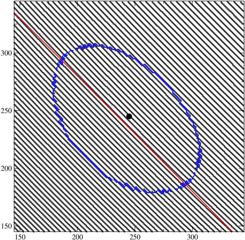
Figure 3: Crests of the Green function $G^{{\cal E}{\cal E}}_{i,j;1}(t)$ for $\rho=0.3$ and $t=1200$. The local wavelength $\overline{\lambda}(v)$ increases between the lower left and the upper right, as predicted by (62). The crests are slightly concave (see section 3.5), as can be seen by comparison with the straight red line $i+j=2v_{\rm g}t$. The amplitude is maximal at the black dot and one tenth of the peak amplitude on the blue curve.

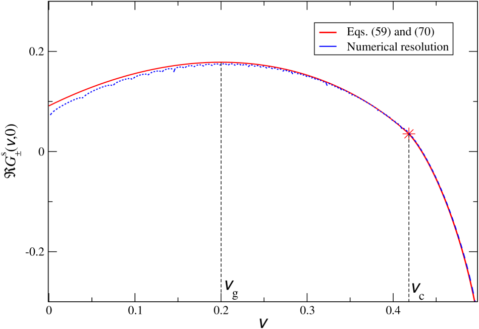
Figure 4: The logarithm $\Re{\cal G}^{\mathrm{s}}_{\pm}(v,0)$ of the envelope of the wave packet along the diagonal $i=j$ for $t=400$ and $\rho=0.3$. Shown are both the analytical prediction (red) from Eqs. (59) and (70) and the numerical solution (blue) of the linearized evolution equations (2)-(6). The red star emphasizes a discontinuity in the slope.

The envelope of (58), determined by (59), peaks at a value $i=j=v_{\rm g}t$ where $v_{\rm g}$ is the solution of $\partial{\cal G}^{\mathrm{s}}_{\pm}/\partial v|_{v_{\rm g}}=0$. The value of $v_{\rm g}$ is interpreted as the projection of the group velocity along the direction $i$ (or $j$), which gives for the true group velocity of the packet $\overline{v}_{\rm g}=\sqrt{2}v_{\rm g}$. We find

$$v_{\rm g}=\frac{c^{2}-1}{2(c^{2}+1)}=\frac{1}{2}-\rho.$$ (63)

This shows that our description makes sense, at best, in the density interval $0<\rho<1/2$. Substitution of (63) in (59) yields a remarkably simple expression for the maximal growth rate $\Re{\cal G}^{\mathrm{s}}_{\pm}(v_{\rm g},0)$,

$$\exp\Re{\cal G}^{\mathrm{s}}_{\pm}(v_{\rm g},0) = (1+c^{-2})^{-1/2}$$ (64)

$$= (1-\rho)^{-1/2},$$

so that $|G^{{\cal E}{\cal E}}_{i,i;j^{\prime}}(t)|\sim(1-\rho)^{-t/2}$ for $i=v_{\rm g}t$ and $t\rightarrow\infty$. This growth rate is identical to the one associated with periodic boundary conditions (Ref. [25], subsection 4.2).

The amplitude of the Green function is shown in figure 4 as a function of $v$, together with its numerical determination. The prefactor has been adjusted to obtain the best agreement between both curves. The maximum occurs at $v=v_{\rm g}=0.2$ [Eq. (63)] and there is a discontinuity in the slope at $v=v_{\rm c}\simeq 0.41833$ [Eq. (56)], which is well brought out numerically.

At the maximum of the peak we have $v=v_{\rm g}$. Using (3.2) and (63) to express $\overline{\lambda}_{\rm 0}=\overline{\lambda}(v_{\rm g})$ as a function only of $\rho$ we thus find from (62) that this wavelength of maximal instability has the expression

$$\overline{\lambda}_{\rm 0} = \sqrt{2}\pi/\arctan\Bigg{(}\frac{\sqrt{3-4\rho}}{1-2\rho}\Bigg{)}$$ (65)

$$= \sqrt{2}\pi/\arccos\Bigg{(}\frac{1-2\rho}{2(1-\rho)}\Bigg{)}.$$

Remarkably, this expression for the most unstable wavelength is is identical to the one found in Ref. [25] for the much simpler case of periodic boundary conditions. This therefore points towards a robust property of the mean field equations. Typically, $\overline{\lambda}_{\rm 0}$ is of the order of three to four lattice spacings. Let $\overline{v}_{{\rm ph},{\rm 0}}=\omega(v_{\rm g})/\overline{k}(v_{\rm g})$ denote the phase velocity of the oscillations inside the wave packet. From Eq. (61) we have

$$\overline{v}_{{\rm ph},{\rm 0}}=\frac{\arctan\sqrt{3-4\rho}}{\sqrt{2}\arccos\bigg{(}\frac{1-2\rho}{2(1-\rho)}\bigg{)}}\,.$$ (66)

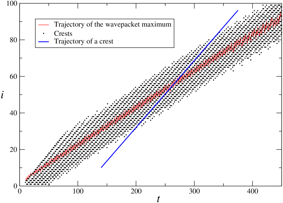
Figure 5: Numerical determination of the crests of the Green function $G^{{\cal E}{\cal E}}$ for $\rho=0.30$ shown in the time-space plane. Positions are shown only of those crests that are within a distance of ten lattice units from the wave packet maximum.

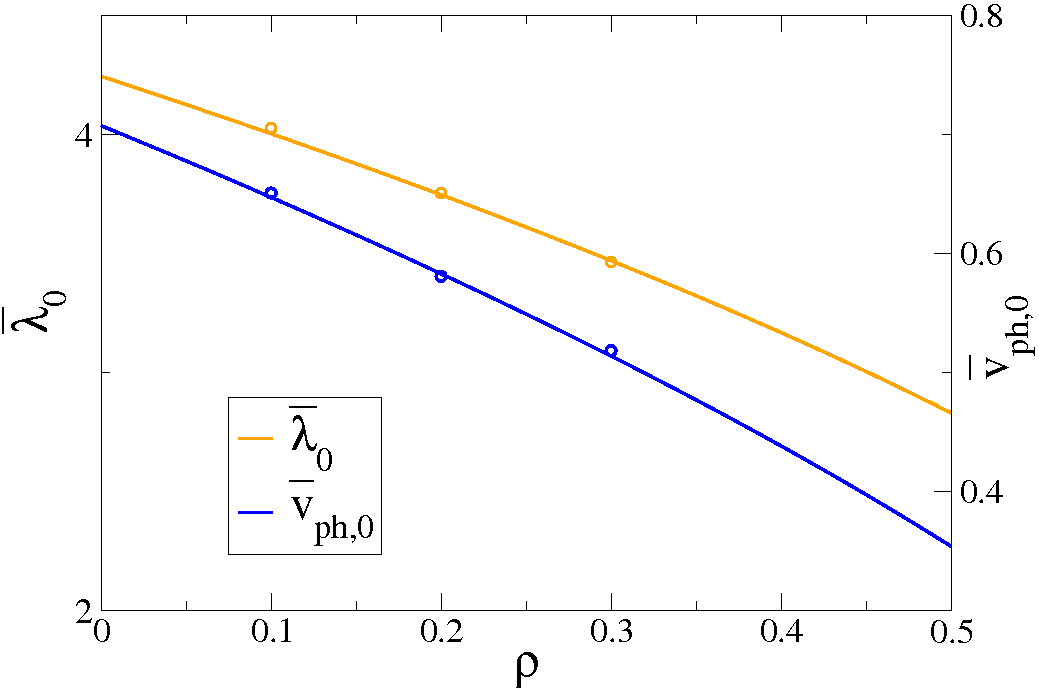
Figure 6: Wavelength $\overline{\lambda}_{\rm 0}$ and phase velocity $\overline{v}_{{\rm ph},{\rm 0}}$ at the maximum of the peak as a function of $\rho$. The lines are the analytic predictions and the dots from numerical determination. The uncertainty comes from the estimation of $\overline{\lambda}_{\rm 0}$ and $\overline{v}_{{\rm ph},{\rm 0}}$ from the numerical data, and in both cases the error bars are smaller than the symbol size.

Figure 5 is based on a numerical determination of the Green function for $\rho=0.30$ along the diagonal $i=j$. The fluctuating (red) solid line represents the trajectory of the maximum of the wave packet in the $ti$ plane. Its fluctuations are due to the incommensurability between the wavelength of the oscillations and the lattice spacing. Its average slope is the projected group velocity $v_{\rm g}$. The black dots are the positions of the crests, limited to those within a distance of ten lattice units from the maximum. In this figure a crest is a lattice site $(i,j)$ such that $p^{\cal E}_{i-1,j-1}<p^{\cal E}_{i,j}>p^{\cal E}_{i+1,j+1}$. The straight (blue) solid line is the trajectory of a given crest in the $ti$ plane. Its slope is the projection of the phase velocity. A few values of $\overline{\lambda}_{\rm 0}$ and $\overline{v}_{{\rm ph},{\rm 0}}$ determined from plots similar to figure 5 are shown in figure 6.

Finally, the width of the peak along the diagonal direction can be calculated as well. Defining

$$\sigma_{\parallel,{\rm 0}}^{2}\equiv\frac{1-4v_{\rm g}^{2}}{4}=\rho(1-\rho),$$ (67)

we have

$$t\Re{\cal G}^{\mathrm{s}}_{\pm}(v,0) = t\Re{\cal G}^{\mathrm{s}}_{\pm}(v_{\rm g},0)-t\frac{(v-v_{\rm g})^{2}}{2\sigma_{\parallel,{\rm 0}}^{2}}+tO((v-v_{\rm g})^{3})$$ (68)

$$= t\Re{\cal G}^{\mathrm{s}}_{\pm}(v_{\rm g},0)-\frac{((i+j-2v_{\rm g}t)/2)^{2}}{2\sigma_{\parallel,{\rm 0}}^{2}t}+O(t^{-2}),$$

which shows that the perturbation spreads diffusively. Eq. (67) is the standard expression for the variance of a Bernoulli distribution of parameter $\rho$. It can be seen in the evolution equations (2) that a perturbation of the density field will increase its value of $i+j$ with probability $1-\rho$ and decrease this value with probability $\rho$ at each time step, which explains the expression (67). This interpretation also explains why the expression (63) for $v_{\rm g}$ becomes negative when $\rho>1/2$. We have verified expression (67) numerically.

Case $v>v_{\rm c}$.    When $v>v_{\rm c}$ the quantity ${V}$ becomes pure imaginary and we define

$$W\equiv-{\mathrm{i}}V=\sqrt{4v^{2}(1+c^{2})-c^{2}},\qquad v>v_{\rm c}\,,$$ (69)

which is real positive, so that both saddle points $R^{\mathrm{s}}_{\theta}$ are now pure imaginary. We direct the path of integration only through $R^{\mathrm{s}}_{+}$, since at this point the direction of negative curvature is parallel to the real axis whereas in $R^{\mathrm{s}}_{-}$ the two directions are perpendicular.

Equations (52) together with (53)-(54) lead to the counterpart of (57),

$${\cal G}^{\mathrm{s}}_{+}(v,0) = \log 2-\log(1+c^{2})+4v\log c-(1-2v)\log(1-2v)-\log(1+2v)$$ (70)

$$+\log(1+W)-2v\log(2v+W),\qquad v>v_{\rm c},$$

The ${\cal G}^{\mathrm{s}}_{\pm}$ are real and the Green function depends exponentially on $t$.

$$G^{{\cal E}{\cal E}}_{i,i;j^{\prime}}(t)\simeq B_{+}\,{\mathrm{e}}^{t{\cal G}^{\mathrm{s}}_{+}(v,0)},\qquad i=vt,\quad v>v_{\rm c}\,,\quad t\to\infty.$$ (71)

Eqs. (70) and (71) together give the envelope of the Green function. This second part of the envelope has also been calculated numerically and is also shown in figure 4. We note that it concerns the front of the wave, where the amplitude is still extremely small compared to its peak value. Numerical and analytic work are in excellent agreement.

3.5 Green function off the diagonal: $i\neq j$

In this last subsection we study the Green function for the case $u\neq 0$. At fixed $v$, varying $u$ corresponds to scanning the Green function along an ‘antidiagonal’ of constant $i+j$. The most interesting case is when $i+j=2v_{\rm g}t$, which is the antidiagonal passing through the peak of the wave packet.

For $u\neq 0$ and $v$ arbitrary the function to study is then the full expression (52). Substitution of Eqs. (53) and (54) in Eq. (52) gives again ${\cal G}^{\mathrm{s}}_{\theta}(v,0)$ of Eq. (57) but augmented with terms of order $u^{2}/t$. Explicitly,

$${\cal G}^{\mathrm{s}}_{\theta}(v,u) = {\cal G}^{\mathrm{s}}_{\theta}(v,0)+\frac{2(1-2v)}{1+2v}\frac{1-{\mathrm{i}}\mathcal{R}_{\theta}}{{\mathrm{i}}\mathcal{R}_{\theta}}\frac{u^{2}}{t}+O(t^{-2})$$ (72)

$$= {\cal G}^{\mathrm{s}}_{\theta}(v,0)-\frac{1}{2}\left(\frac{1}{\sigma_{\perp}^{2}}+{\mathrm{i}}\theta\phi^{\prime\prime}\right)\frac{u^{2}}{t}+O(t^{-2}).$$

The real term gives the transverse width of the wave packet. Using the explicit expression (45) for $\mathcal{R}_{\theta}$ we find

$$\sigma_{\perp}^{2}=\frac{c^{2}-4v^{2}}{4c^{2}}\frac{1+2v}{1-2v}.$$ (73)

The imaginary term is in fact the second derivative of the phase of the cosine in equation (58) with respect to $u$ and reads

$$\phi^{{\prime\prime}}=\frac{4V(1-2v)}{(1+2v)(c^{2}-4v^{2})}\,,$$ (74)

in which $V$ is given by (3.2). By combining again the results from the two saddle points $\theta=\pm 1$ we find that, to second order in $u$ around the diagonal, the wave packet is given by a generalization of (58),

$$G^{{\cal E}{\cal E}}_{i,j;j^{\prime}}(t) \simeq 2B\,{\mathrm{e}}^{t\Re{\cal G}^{\mathrm{s}}_{+}(v,0)}{\mathrm{e}}^{-u^{2}/(2\sigma_{\perp}^{2})}\cos\bigg{(}\omega t-\frac{1}{2}(i+j)k+\phi+\frac{\phi^{{\prime\prime}}}{2}u^{2}\bigg{)},$$ (75)

$$i,j=vt\pm ut^{1/2},\quad v<v_{\rm c}\,,\quad t\to\infty,$$

where $\Re{\cal G}^{\mathrm{s}}_{+}(v,0)$, $\omega(v)$, and $k(v)$ are given by expressions (59)and (61) of subsection 3.4. By substituting in (73) and (74) the expressions for $v_{\rm g}$ and $c$ in terms of $\rho$ one finds, in obvious notation,

$$\sigma_{\perp,{\rm 0}}^{2}=\frac{1-2\rho+4\rho^{2}-4\rho^{3}}{4\rho}=\rho(1-\rho)+\frac{1-2\rho}{4\rho}\,.$$ (76)

and

$$\phi^{{\prime\prime}}_{\rm 0}=\frac{4\rho^{2}\sqrt{3-4\rho}}{(1-\rho)(1-2\rho+4\rho^{2}-4\rho^{3})}\,.$$ (77)

From equations (67) and (76) we notice that the variance in the antidiagonal direction $\sigma_{\perp,{\rm 0}}$ is always larger than its diagonal counterpart, in accordance with the scheme drawn in figure 2. According to Eq. (75) the Green function should vanish every time the cosine in that equation has a zero.

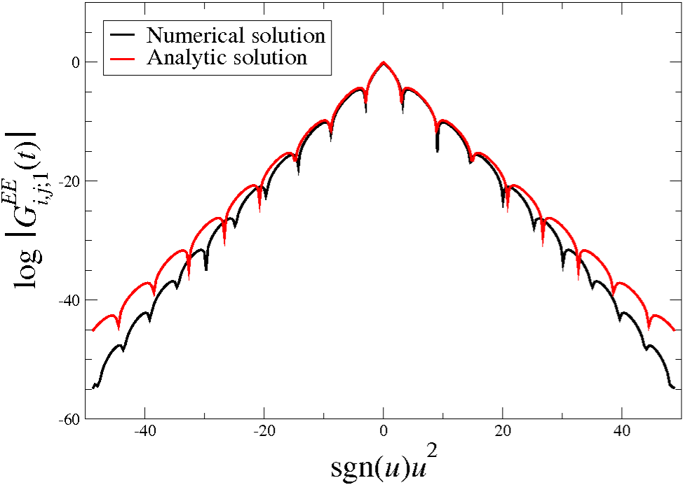
Figure 7: Logarithm of the Green function $G^{{\cal E}{\cal E}}_{i,j;1}(t)$ for $i,j=v_{\rm g}t\pm u\sqrt{t}$, evaluated for $\rho=0.30$ at time $t=1200$. The black curve is the numerical solution and the red one is the analytic expression (75). Both curves have been shifted so that they have unit amplitude in $u=0$, and the value of $\phi$ in the analytic expression has been fitted.

In figure 7 we show the Green function $G^{{\cal E}{\cal E}}_{i,j;1}$ along the antidiagonal $i+j=2v_{\rm g}t$, that passes through the peak of the wave packet, as a function of $u=(i-j)/(2\sqrt{t})$. The downward dips are the divergences of $\log|G^{{\cal E}{\cal E}}_{i,j;1}|$ that occur when the cosine in (75) vanishes. There is excellent agreement for smal $u$ values; since the analytic expression is based on a small-$u$ expansion, it is normal that for larger $u$ deviations appear.

Whereas the term $(i+j)k/{2}$ in the argument of the cosine in (75) suggests the propagation of plane waves in the $(1,1)$ direction, the term $\frac{\phi^{{\prime\prime}}}{2}u^{2}$ induces a very slight curvature, which is nevertheless clearly visible in figure 3.

This effect is theoretically very interesting and we are not aware of any intuitive explanation. Since it appears in the wings of the wavepacket where the amplitude is very small, it will be washed out when the Green function is convoluted with the space and time dependent noise at the entrance boundaries. It might however be observable under idealized circumstances with a pure ’instanton’ perturbation of a homogeneous flow. We note that this curvature effect is not related to a different curvature phenomenon, termed the chevron effect, that we discovered and described in earlier work [24, 25] and that appears once a stationary state has set in under the influence of the nonlinear terms in the equations. The chevron effect is essentially nonlinear; no evidence of it was found in the initial linear regime studied in this work.

This completes the asymptotic analysis of the Green function $G^{{\cal E}{\cal E}}$. The same asymptotic arguments can be applied to $G^{{\cal E}{\cal N}}$, which differs from $G^{{\cal E}{\cal E}}$ only by a factor $\big{(}\frac{\zeta a_{p}}{c}\big{)}^{2}$ in the integrand and a relabeling of the indices. In particular the shape of the peak and the wavelength of the oscillations are the same as those found for $G^{{\cal E}{\cal E}}$. The two other Green functions $G^{{\cal N}{\cal E}}$ and $G^{{\cal N}{\cal N}}$ are obtained by exchanging $({\cal E},i)$ with $({\cal N},j)$.

4 Summary and conclusion

We have studied the stripe formation instability known to occur in the crossing area of two perpendicular traffic flows (‘eastward’ and ‘northward’) through streets of suffcient width. The phenomenon is common to a wide class of models. In the present work the two streets were modeled as strips of a square lattice of width $M$. We have started from the deterministic nonlinear mean-field flow equations (1) whose unknowns are the space and time dependent densities $\rho^{\cal E}_{i,j}$ and $\rho^{\cal N}_{i,j}$ of the eastbound and northbound traffic, respectively. These nonlinear equations cannot be solved analytically. In earlier work [25] we therefore performed a Monte Carlo study of the stationary states of these equations, which are unstable to the appearance of a fully developed striped pattern. Here our purpose has been to study the initial linear  growth of this instability and to show that it may be triggered by random open boundary conditions (OBC), representing randomly incoming traffic at the west and south entrance boundaries of the crossing area. The same instability was also studied analytically ([25], section 4) in the more artificial geometry of periodic boundary conditions (PBC) and subject to a random initial condition. For the linear problem (2) at hand all information is contained in the Green functions. Their expressions can be calculated exactly via  diagonalization of the time evolution matrix and are given by Eqs. (28)-(29) as a double sum of an integral. We have evaluated these asymptotically in the limit of large times and shown that the Green function represents a wave packet of growing amplitude that propagates along the $(1,1)$ direction.

For the traveling wave packet generated by an instantaneous point-like disturbance on one of the boundaries, we found explicit expressions for the wavelength $\overline{\lambda}_{\rm 0}$ of maximum instability as a function of the average traffic density $\rho$, for the growth rate of the instability, and for the group and phase velocities, $\overline{v}_{\rm g}$ and $\overline{v}_{{\rm ph},{\rm 0}}$, respectively. We found full agreement between our analytic results and a numerical determination of the Green function.

We concluded that random entrance boundary conditions (OBC) generate a wave pattern similar to the one found under the much simpler PBC. This result is interesting and important for the analysis of similar models. It shows that the simplified version of a model with PBC and random initial conditions may quite well replace the full model as far as the features studied here are concerned. Nevertheless, the calculation of the Green function of the full model with OBC, as carried out in this work, gives a much deeper insight into the interaction between the two crossing flows, the selection mechanism of the dominant mode of propagation, and the different time scales involved. It has brought to light an interesting curvature effect of the wavefront in the wings of the wave packet, created by an instanton perturbation. Furthermore, the knowledge about the Green function that we have acquired here may be applied directly, by means of a simple convolution, to more complicated cases with arbitrary boundary conditions in which the entrance noise may or may not have correlations. It is very likely, moreover, that our method can be extended to various other situations that may arise.

References

• [1] K. Nagel, M. Schreckenberg, A cellular automaton model for freeway traffic, J. Physique I 2 (1992) 2221–2229.
• [2] M. E. Foulaadvand, Z. Sadjadi, M. R. Shaebani, Optimized traffic flow at a single intersection: traffic responsive signalization, J. Phys. A: Math. Gen. 37 (2004) 561–576.
• [3] M. E. Foulaadvand, M. Neek-Amal, Asymmetric simple exclusion process describing conflicting traffic flows, Europhys. Lett. 80 (2007) 60002.
• [4] H.-F. Du, Y.-M. Yuan, M.-B. Hu, R. Wang, R. Jiang, Q.-S. Wu, Totally asymmetric exclusion processes on two intersected lattices with open and periodic boundaries, J. Stat. Mech. (2010) P03014.
• [5] C. Appert-Rolland, J. Cividini, H. J. Hilhorst, Intersection of two TASEP traffic lanes with frozen shuffle update, J. Stat. Mech. (2011) P10014.
• [6] T. Naka, Mechanism of cross passenger flow, Transactions of the Architectural Institute of Japan 258 (1977) 93–102.
• [7] K. Ando, H. Ota, T. Oki, Forecasting the flow of people, Railway Research Review 45 (1988) 8–14.
• [8] S. P. Hoogendoorn, W. Daamen, Self-organization in walker experiments, in: S. Hoogendoorn, S. Luding, P. Bovy, et al. (Eds.), Traffic and Granular Flow ’03, Springer, 2005, pp. 121–132.
• [9] M. Plaue, M. Chen, G. Bärwolff, H. Schwandt, Trajectory extraction and density analysis of intersecting pedestrian flows from video recording, in: U. Stilla, F. Rottensteiner, H. Mayer, B. Jutzi, M. Butenuth (Eds.), Photogrammetric Image Analysis, Vol. 6952, Springer Berlin Heidelberg, 2011, pp. 285–296.
• [10] J. Bamberger, A.-L. Geßler, P. Heitzelmann, S. Korn, R. Kahlmeyer, X. H. Lu, Q. H. Sang, Z. J. Wang, G. Z. Yuan, M. Gauß, T. Kretz, Crowd research at school: Crossing flows, arXiv:1401.2038.
• [11] S. Hoogendoorn, P. H. L. Bovy, Simulation of pedestrian flows by optimal control and differential games, Optim. Control Appl. Meth. 24 (2003) 153–172.
• [12] K. Yamamoto, M. Okada, Continuum model of crossing pedestrian flows and swarm control based on temporal/spatial frequency, in: 2011 IEEE International Conference on Robotics and Automation, 2011, pp. 3352–3357.
• [13] O. Biham, A. Middleton, D. Levine, Self-organization and a dynamic transition in traffic-flow models, Phys. Rev. A 46 (1992) R6124–R6127.
• [14] S.-I. Tadaki, Two-dimensional cellular automaton model of traffic flow with open boundaries, Phys. Rev. E 54 (1996) 2409–2413.
• [15] M. S. Watanabe, Dynamical behaviour of a two-dimensional cellular automaton with signal processing, Physica A 324 (2003) 707–716.
• [16] M. S. Watanabe, Dynamical behaviour of a two-dimensional cellular automaton with signal processing. (II). Effect of signal period, Physica A 328 (2003) 251–260.
• [17] M. Fukui, Y. Ishibashi, Two-dimensional city traffic model with periodically placed blocks, Physica A 389 (2010) 3613–3618.
• [18] Z. Xiao-mei, X. Dong-fan, J. Bin, J. Rui, G. Zi-you, Disorder structure of freee-flow and global jams in the extended bml model, Phys. Lett. A 3775 (2011) 1142–1147.
• [19] Z.-J. Ding, R. J., B.-H. Wang, Traffic flow in the Biham-Middleton-Levine model with random update rule, Phys. Rev. E 83 (2011) 047101.
• [20] Z.-J. Ding, R. Jiang, W. Huang, B.-H. Wang, Effect of randomization in the Biham-Middleton-Levine traffic flow model, J. Stat. Mech. (2011) P06017.
• [21] Z.-J. Ding, R. Jiang, M. Li, Q.-L. Li, B.-H. Wang, Effect of violating the traffic light rule in the Biham-Middleton-Levine traffic flow model, Europhys. Lett. 99 (2012) 68002.
• [22] Q.-H. Sui, Z.-J. Ding, R. Jiang, W. Huang, D. Sun, B.-H. Wang, Slow-to-start effect in two-dimensional traffic flow, Computer Physics Communications 183 (2012) 547–551.
• [23] M. Muramatsu, T. Nagatani, Jamming transition of pedestrian traffic at a crossing with open boundaries, Physica A 286 (2000) 377–390.
• [24] J. Cividini, C. Appert-Rolland, H. J. Hilhorst, Diagonal patterns and chevron effect in intersecting traffic flows, Europhys. Lett. 102 (2013) 20002.
• [25] J. Cividini, H. J. Hilhorst, C. Appert-Rolland, Crossing pedestrian traffic flows,diagonal stripe pattern, and chevron effect, J. Phys. A: Math. Theor. 46 (2013) 345002.
• [26] J. Cividini, C. Appert-Rolland, Wake-mediated interaction between driven particles crossing a perpendicular flow, J. Stat. Mech. (2013) P07015.
• [27] H. J. Hilhorst, J. Cividini, C. Appert-Rolland, Continuous and first-order jamming transition in crossing pedestrian traffic flows, in: Perspectives and Challenges in Statistical Physics and Complex Systems for the Next Decade, World Scientific, 2014.
• [28] M. Moussaïd, E. Guillot, M. Moreau, J. Fehrenbach, O. Chabiron, S. Lemercier, J. Pettré, C. Appert-Rolland, P. Degond, G. Theraulaz, Traffic instabilities in self-organized pedestrian crowds, PLoS Computational Biology 8 (2012) 1002442.
• [29] J. Dzubiella, G. P. Hoffmann, H. Löwen, Lane formation in colloidal mixtures driven by an external field, Phys. Rev. E 65 (2002) 021402.
• [30] J. Zhang, A. Seyfried, Comparison of intersecting pedestrian flows based on experiments, Physica A 405 (2014) 316–325.