Environment fluctuations on single species pattern formation

Abstract

System-environment interactions are intrinsically nonlinear and dependent on the interplay between many degrees of freedom. The complexity may be even more pronounced when one aims to describe biologically motivated systems. In that case, it is useful to resort to simplified models relying on effective stochastic equations. A natural consideration is to assume that there is a noisy contribution from the environment, such that the parameters which characterize it are not constant but instead fluctuate around their characteristic values. From this perspective, we propose a stochastic generalization of the nonlocal Fisher-KPP equation where, as a first step, environmental fluctuations are Gaussian white noises, both in space and time. We apply analytical and numerical techniques to study how noise affects stability and pattern formation in this context. Particularly, we investigate noise induced coherence by means of the complementary information provided by the dispersion relation and the structure function.

I Introduction

The mathematical description of the spatial distribution of biological populations can be achieved on a phenomenological mesoscopic level where system and environment properties are typified by means of a few control parameters. The evolution of a population distribution is mainly ruled by processes such as reproduction Malthus (1993) and (interspecific or intraspecific) competitions, which are usually mimicked by logistic-like expressions Verhulst (1838), together with spatial dispersal, modeled by (normal or anomalous) diffusion. Then, the population characteristics and the coupling to the environment are quantified by a set of control parameters, such as growth rate, carrying capacity and diffusion coefficient, each one assigned a typical value. Such simple models allow to predict the relaxation towards a steady state, resulting from the interplay between the population growth and the competition for resources in the limited support provided by the environment. However, the long-time evolution of biological populations can present complex spatiotemporal patterns, a signature of self-organization, as can be observed in populations of slime mold, bacteria, ants, birds, fishes and human beings Theraulaz et al. (2002); Toner and Tu (1995); Rudge et al. (2013); Alim et al. (2013); Castellano et al. (2009). Self-organization may arise due to nonlocal interactions Murray (2002); Fuentes et al. (2004, 2003); da Cunha et al. (2011); Clerc et al. (2010) or other mechanisms that drive the system far from equilibrium towards a spatiotemporal organization. As an example, in a recent study about the Allee effect Stephens and Sutherland (1999), it has been shown that the interplay between nonlocality and nonlinearity can lead to the emergence of localized structures Clerc et al. (2010).

The environment certainly interferes in most of those processes. For example, for microorganisms, the environment temperature can affect the reproduction rate Ratkowsky et al. (1982) and many other processes Farrell and Rose (1967) such as spatial spread. Competition is intrinsically mediated by the environment due to its limited resource availability (carrying capacity) Verhulst (1838). Now, due to the inherent complexity, an environment parameter is typically subjected to a complex web of diverse processes, varying at different scales, both in space and time. Therefore, it would be more realistic to model its complicated behavior by means of a stochastic variable. It is our goal to investigate the impact of such fluctuations on population dynamics. We will consider a single species scenario in one-dimension for the evolution of the population density $u(x,t)$.

A standard deterministic model that takes into account the above mentioned governing rules is the generalized Fisher-KPP equation Kolmogorov et al. (1937); Fisher (1937); Fuentes et al. (2003), namely, the adimensionalized integro-differential equation

$$\frac{\partial u(x,t)}{\partial t}=a\,u(x,t)-b\,u(x,t)\,\mathcal{J}[u](x,t)+D\frac{\partial^{2}}{\partial x^{2}}u(x,t)\,,$$ (1)

where $\{a,b,D\}$ are positive parameters and $\mathcal{J}[u](x,t)=\int_{\Omega}f(x-x^{\prime})u(x^{\prime},t)dx^{\prime}$, with $f$ a function that describes the influence of two interacting infinitesimal elements at a distance $x-x^{\prime}$. The first term in Eq. (1) accounts for the balance between the birth and death rates and the second one introduces a nonlocal intraspecific competition that sets a saturation limit on population growth. Then they can be seen as a generalization of the Verhulst expression. The last term introduces spatial spread through normal diffusion Murray (2003).

In Eq. (1), the environment participates in defining all the set of control parameters $\{a,b,D\}$. The inclusion of small fluctuations (or noise) allows to reflect the spatiotemporal variability of the complex environment. We focus on the effects of the multiplicative noise that arises by resorting to the transformation $a\rightarrow a+\sigma_{\eta}\eta(x,t)$, and we also consider the impact of an additive noise $\sigma_{\xi}\xi(x,t)$, where $\sigma_{\eta}$ and $\sigma_{\xi}$ are constant parameters that control the amplitude of the fluctuations, and where both $\xi$ and $\eta$ are independent Gaussian noises, with null averages $\langle\eta(x,t)\rangle=\langle\xi(x,t)\rangle=0$, and white in space-time, i.e., $\langle\eta(x,t)\eta(x^{\prime},t^{\prime})\rangle=\delta(x-x^{\prime})\delta(t-t^{\prime})$ and $\langle\xi(x,t)\xi(x^{\prime},t^{\prime})\rangle=\delta(x-x^{\prime})\delta(t-t^{\prime})$. In the context of population dynamics these multiplicative and additive fluctuations introduce the complex aspects of the environment in the growth rate and in the flux of individuals through the system boundaries, respectively.

Therefore, our object of study is the dynamical equation that can be cast in the following form:

$$\frac{\partial u(x,t)}{\partial t} = {\bigl{(}a+\sigma_{\eta}\eta(x,t)\bigr{)}}u(x,t)+\sigma_{\xi}\xi(x,t)+$$ (2)

$$-bu(x,t)\mathcal{J}[u]+D\frac{\partial^{2}}{\partial x^{2}}u(x,t)\;.$$

Since the shape of the influence function does not lead to substantially different results Fuentes et al. (2003), for the sake of simplicity, throughout this work we will use a Heaviside influence function defined as $f(x-x^{\prime})=\frac{1}{2w}\Theta(w-|x-x^{\prime}|)$. In the previous expression, $w$ is a positive constant, defining the range of the interactions.

Moreover, for the multiplicative white noise term, one must state an additional prescription (typically, either Itô or Stratonovich) Kampen (1981). Within the present scenario, there are cases in which the Itô interpretation is suitable, for example i) when the environment is sensed in a nonantecipative manner by the individuals Turelli (1977), ii) when the continuous model is actually an approximation for a discrete time population evolution Lande (1993), or iii) when fluctuations originate from internal sources. On the other hand, if fluctuations are external, the Stratonovich description is more appropriate. This is so because in the latter case the deterministic drift is recovered in the limit of vanishing fluctuations, while the drift is coupled to the fluctuations when they have internal origin Kampen (1981). Since both rules may be sound depending on the specific environment fluctuations taken into account, we will consider both of them, making a comparison of their different effects while the model parameters are kept the same. This is the way we chose to present the results, despite formally a correspondence between both descriptions will ultimately amount to the modification of the deterministic term.

The effects of additive noise in spatially extended systems have been tackled by previous works (for example see Refs. Sagués et al. (2007); Agez et al. (2013); Ridolfi et al. (2011)). Now, we analyze these effects in the context of population dynamics. The additive noise accounts for the effect of a system-environment coupling that is density-independent. Additive fluctuations represent fluctuating fluxes of individuals through the system’s boundary. Then, even when the population tends to vanish, a positive fluctuation represents a reintroduction of individuals into the system, spoiling the absorbent state. A negative value of the noise reflects a tendency to an outwards flux. But, this can be accomplished only until a null value of $u$ is attained, then in numerical solutions, at each step, we trimmed fluctuations that would lead to a negative value of $u$. In fact, additive noise in Eq. (2) compromises the positivity of the population density, therefore the stochastic equation must be complemented by an additional mathematical constraint, as the one chosen, to forbid negative values of $u$.

II Instability conditions

In the deterministic case Fuentes et al. (2003), i.e. when $\sigma_{\xi}=\sigma_{\eta}=0$, one can determine the instability condition for the emergence of periodic structures by following the standard procedure of linearizing Eq. (1) around the homogeneous solution $u_{0}=a/b$, assuming $u(x,t)=u_{0}+\varepsilon(x,t)$, where $\varepsilon(x,t)=\varepsilon_{0}\exp[ikx+\lambda(k)t]$ is a small perturbation around the uniform state $u_{0}$. This procedure leads to the dispersion relation

$$\lambda(k)=-a\tilde{f}(k)-Dk^{2}\,,$$ (3)

where $\tilde{f}$ is the Fourier transform of the influence function, that in the particular case of the Heaviside influence becomes $\tilde{f}(k)=\sin{(wk)}/[wk]$. The relation (3) indicates instability with respect to a certain mode $k$, if $\lambda(k)>0$. Then, in general, patterns are expected if the dispersion relation satisfies two conditions: (i) $\lambda(0)<0$, to avoid instability of the average population size, and (ii) there must exist a positive global maximum at certain $k^{*}>0$ Cross and Hohenberg (1993), to give rise to an emergent characteristic mode. Recently, it has been shown that this relation provides important information about the pattern formation process not only for short times but also asymptotically, as soon as mode coupling is weak Colombo and Anteneodo (2012). In particular, diffusion has a stabilizing role, while the first term has not a definite sign. Following the dispersion relation (3), we show in Fig. 1 that, when the diffusion coefficient is reduced with the other parameters kept constant, the homogeneous solution can become unstable and patterns emerge in the population Fuentes et al. (2003); Colombo and Anteneodo (2012). Both instances are depicted in Fig. 1, for fixed parameters $a,b,w$. Notice that in both cases $\lambda(0)<0$, but, for small $D$, $\lambda(k)$ takes positive values, while for $D$ above a threshold value $\lambda(k)$ is always negative indicating the stability of the homogeneous state.

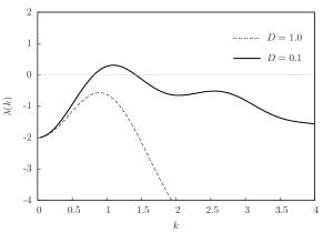
Figure 1: Dispersion relation given by Eq. (3), for $a=2$, $b=1$, $w=4$, and two values of the diffusion coefficient $D$ indicated on the figure.

Now let us turn to the stochastic version of the nonlocal Fisher-KPP equation. By linearizing Eq. (2) around $u_{0}=a/b$, in the small noise approximation, we have

$$\frac{\partial\varepsilon(x,t)}{\partial t} =\;-a\mathcal{J}[\varepsilon](x,t)+D\frac{\partial^{2}}{\partial x^{2}}\varepsilon(x,t)+$$

$$+\sigma_{\eta}\varepsilon(x,t)\eta(x,t)+\sigma_{\eta}u_{0}\eta(x,t)+\sigma_{\xi}\xi(x,t)\,,$$ (4)

where the deterministic terms are represented in the first line of the right hand side of Eq. (II), while the second line contains the multiplicative and additive noise terms. A suitable way to verify pattern formation is to measure the spatial autocovariance $C(r,t)=\int\langle\varepsilon(x,t)\varepsilon(x+r,t)\rangle dx$ (which does not depend on $t$ if stationarity holds) or, alternatively, its Fourier transform, that is the structure function

$$S(k,t)\equiv\left\langle\hat{\varepsilon}(k,t)\hat{\varepsilon}(-k,t)\right\rangle\,,$$ (5)

where $\hat{\varepsilon}$ is the Fourier transform of $\varepsilon$.

Following the lines of Refs. Ridolfi et al. (2011); Ibañes et al. (2000), we derive the evolution equation of $S(k,t)$ under the Stratonovich interpretation. Starting from the Fourier transform of Eq. (II), considering $\partial_{t}(\hat{\varepsilon}\hat{\varepsilon}^{\prime})=\hat{\varepsilon}\partial_{t}(\hat{\varepsilon}^{\prime})+\hat{\varepsilon}^{\prime}\partial_{t}(\hat{\varepsilon})$, where $\hat{\varepsilon}\equiv\hat{\varepsilon}(k,t)$ and $\hat{\varepsilon}^{\prime}\equiv\hat{\varepsilon}(-k,t)$, and averaging, we obtain

$$\frac{1}{2}\frac{\partial}{\partial t}S(k,t)=\lambda(k)S(k,t)+\sigma_{\eta}\langle\hat{\varepsilon}^{\prime}\widehat{\varepsilon\eta}\rangle+\sigma_{\eta}u_{0}\langle\hat{\varepsilon}^{\prime}\hat{\eta}\rangle+\sigma_{\xi}\langle\hat{\varepsilon}^{\prime}\hat{\xi}\rangle\,.$$ (6)

In order to evaluate the average of multiplicative terms, we resort, for the case of the Stratonovich interpretation, to the so-called Furutsu-Novikov theorem Novikov (1965), namely

$$\langle\chi(q)g[\chi]\rangle=\int dy\langle\chi(q)\chi(y)\rangle\left\langle\frac{\delta\left[g(q)\right]}{\delta\chi(y)}\right\rangle\,,$$ (7)

where $g(q^{\prime})$ is functionally dependent on the Gaussian stochastic process $\chi$. Hence, the averages of interest, in the small noise approximation, are

$$2\langle\hat{\varepsilon}^{\prime}\widehat{\varepsilon\eta}\rangle =\sigma_{\eta}K_{\eta}S(k,t)\,,$$ (8)

$$2\langle\hat{\varepsilon}^{\prime}\hat{\eta}\rangle =\sigma_{\eta}u_{0}\,,$$ (9)

$$2\langle\hat{\varepsilon}^{\prime}\hat{\xi}\rangle =\sigma_{\xi}\,,$$ (10)

where $K_{\eta}$ is to be interpreted as the spatial correlation function of the noise for $x=x^{\prime}$, numerically computed as $K_{\eta}=1/\Delta x$, where $\Delta x$ is the lattice spacing.

Finally, substituting the averages into Eq. (6), the dynamical equation for the structure function reads

$$\frac{\partial}{\partial t}S(k,t)=2\Lambda_{\nu}(k)S(k,t)+\sigma_{\eta}^{2}u_{0}^{2}+\sigma_{\xi}^{2}\,,$$ (11)

with

$$\Lambda_{\nu}(k)=-a\tilde{f}(k)-Dk^{2}+\frac{1}{2}\nu\sigma_{\eta}^{2}K_{\eta}\,,$$ (12)

where, the factor $\nu$ allows to select either the Itô ($\nu=0$) or Stratonovich ($\nu=1$) rules. The former case is obtained either by including the spurious drift to the original equation to transform the noise into a Stratonovich one or simply by considering that the average of multiplicative noise terms vanish.

Notice that Eq. (12) can be identified as the stochastic generalization of the dispersion relation given by Eq. (3). If $\Lambda_{\nu}(k)$ is positive in some range of $k$, then perturbations grow, indicating that the homogeneous state $u_{0}$ is unstable. Otherwise, i.e., if $\Lambda_{\nu}(k)<0$ for all $k$, the state $u_{0}$ is stable and perturbations vanish. The contribution of noise is given by the last term in Eq. (12), that is always nonnegative and independent on $k$. No such effect is predicted when noise is interpreted under the Itô rule ($\nu=0$). In any case, the additive noise does not affect the dispersion relation. Also notice that, although the multiplicative noise $\eta$ is destabilizing in the Stratonovich case, it will affect all modes. Then, the dispersion relation obtained by the linear analysis already points out that noise can reveal the instability built by the nonlocal competitive interactions.

Additional information can be obtained from the structure function. Under stationarity, Eq. (11) leads to

$$S(k)=\frac{\sigma_{\eta}^{2}u_{0}^{2}+\sigma_{\xi}^{2}}{-2\Lambda_{\nu}(k)}\,.$$ (13)

Therefore, although the analysis of the signal of $\Lambda_{\nu}(k)$ predicts no effects caused by noise under the Itô prescription, the structure function reveals that noise can induce some kind of coherence. The numerical analysis in the next sections will clarify this issue.

However, let us remark that the stationary amplitude, $S^{\star}\equiv S(k^{\star})$, of the dominant mode $k^{\star}$ grows with both noise intensities. Moreover, note that $k^{\star}$ is defined by the deterministic component only, hence by the dispersion relation (3). It is in that sense that noise reveals the instability of a hidden dominant mode that has been built by the nonlocal interactions and suppressed by the homogenizing diffusion process. It is also noteworthy that, according to Eq. (13), noise has a constructive role only if $u_{0}>0$. The role of noise as a precursor phenomenon and as a factor that induces coherence is already known in other dynamical systems Sagués et al. (2007); Schöpf and Zimmermann (1993); Carrillo et al. (2004); Agez et al. (2013). In the following section we analyze the impact of noise in the context of Eq. (2).

III Impact of noise

The above analytical statements allow to predict the stability of the homogeneous state in the presence of noise in the dynamic rules. That analysis tacitly assumes the stability of the homogeneous distribution in the absence of noise, i.e., $\lambda(k)<0$ for all $k$, a situation that will be numerically investigated in subsection III.2. We study the impact of noise on deterministically induced patterns ($\lambda(k^{\star})>0$), in subsection III.1.

In order to go beyond the small noise and linear approximations and shed light on the far from equilibrium and nonlinear dynamics, we perform numerical integration of Eq. (2). We follow the Heun algorithm for stochastic equations Sagués et al. (2007), discretizing space and time, with $\Delta x=10^{-1}$ and $\Delta t<10^{-3}$. We use a one-dimensional array, to represent a system of size $L=100$, with periodic boundary conditions.

In all cases, we quantify spatial coherence, at a given time $t$, by means of the structure function, which is an ensemble average. Averages over 100 samples were considered. From the structure function, one can extract the dominant mode $k^{\star}$ and its corresponding amplitude. After a transient period, the stationarity of the structure function is attained. The stationary characteristic mode is well predicted by Eq. (13), as illustrated in Fig. 2 where we show a comparison between the numerical result for the stationary structure function and the linear theory prediction for the Itô case, given by Eq. (13) with $\nu=0$. For Stratonovich, the scenario is qualitatively similar, as soon as the noise intensity is small enough. Through numerical simulations, one can observe that the dominant mode $k^{\star}$ adopts a typical value, in the whole noise intensity range, showing that the uncorrelated noise introduced in the dynamics appears in a correlated manner.

The maximum value $S^{\star}=S(k^{\star})$ gives a measure of the intensity of the dominant mode. In the inset of Fig. 2 we show a normalized histogram of $S^{\star}_{1}$ for an individual realization. Then, although there exists a good agreement between the numerical structure function and its theoretical prediction, there is a large dispersion as depicted by means of an individual realization (dotted line) and also by the distribution of values of $S_{1}^{\star}=S_{1}(k^{\star})$, where $S_{1}(k)$ is the power spectrum of each single realization.

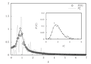
Figure 2: Stationary structure function $S(k)$, for $a=2$, $b=1$, $w=4$, $D=1$, $\sigma_{\xi}=0$ and $\sigma_{\eta}=0.5$ (Itô noise), obtained numerically (symbols) and through Eq. (13) with $\nu=0$ (solid line). For comparison, we also display the stationary power spectrum for an individual realization $S_{1}(k)$ (dotted line). The inset shows the distribution of values of $S_{1}^{\star}=S_{1}(k^{\star})$: numerical (symbols) and gamma distribution fit as a guide to the eyes (solid line).

The structure function $S$ provides full information about spatial coherence. We use its maximum value $S^{\star}$ to quantify coherence through a single variable, but some warnings are required for a proper interpretation. We remark that, even when $S^{\star}$ allows to detect a characteristic scale, at high noise intensity, $S$ tends to flatten as more modes become activated, then patterns become noisier. Furthermore, the structure function measures coherence in Fourier space, and it does not guarantee that patterns are persistent in position space. In subsection III.2 we shall explore this aspect, by directly measuring the temporal correlation and its dependency on noise intensity.

III.1 On deterministically induced patterns ($\lambda(k^{\star})>0$)

Let us consider values of the parameters for which patterns arise in the absence of noise. Then, we use for instance the same values of the solid line in Fig. 1. We discuss spatial coherence as a function of noise intensity mainly through the steady value of $S^{\star}$. We also observe the spatial average density $\langle u\rangle$. By means of numerical simulations, we will go beyond the linear approximation to explore the large fluctuations limit. We first analyze the effect of multiplicative noise (with $\sigma_{\xi}=0$), under both Itô and Stratonovich prescriptions.

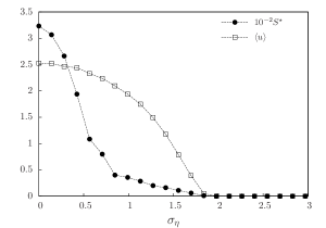
Figure 3: Analysis of the spatial coherence. Steady values of the intensity of the dominant mode $S^{\star}=S(k^{\star})$ and of the average population density, $\langle u\rangle$, as a function of $\sigma_{\eta}$ (under the Itô prescription), for the choice: $a=2$, $b=1$, $w=4$, $D=0.1$ and $\sigma_{\xi}=0$. The intensity of the dominant mode was scaled by a factor $10^{-2}$ just to employ a unique axis scale. The dotted lines are guides to the eyes.

Let us start by the Itô case. In Fig. 3, we represent the steady value of the spatial average density $\langle u\rangle$, together with $S^{\star}$. The results show that multiplicative noise plays a destructive role. Both quantities decay with noise intensity $\sigma_{\eta}$. Moreover, for the set of parameters chosen, there exists a threshold value, $\sigma_{\eta}^{e}\approx 1.8$ in the case of the figure, that represents the extinction threshold. This means that, for noise intensities greater than the threshold, the population becomes extinguished. This implies a shift transition Horsthemke and Lefever (2006) for the critical growth rate that now competes with noise. This effect may be attributed to the fact that the effective growth rate $a+\sigma_{\eta}\eta$ can take negative values. In such case, the shape of the effective drift potential changes so that the null state can become instantaneously stable. This becomes more frequent as the noise amplitude becomes comparable to $a$, then creating a bias towards low densities until extinction. It is noteworthy that, in the local mean-field approximation described by the equation $du/dt=(a-bu)u+\sigma\eta u$, the ensemble average stationary density is given by $\bar{u}=a/b-\sigma^{2}/(2b)$, indicating the existence of a critical threshold. When $\lambda(k^{\star})>0$, through the deterministic mechanisms the system would go towards a stationary state that is represented by a well defined population distribution pattern, meanwhile the presence of multiplicative noise in the dynamic forces, even at low intensity, spoils that spatial order.

In the Stratonovich case, we observe a quite different behavior, as displayed in Fig. 4. Increasing the noise intensity $\sigma_{\eta}$ induces growth both of the average level and of the intensity of the dominant mode, in such a way that also the ratio $S^{*}/\langle u\rangle$ increases. However, as shown in the inset of the same figure, while the amplitude of the patterns grows with increasing noise, their shape becomes more irregular, indicating that the other modes also grow together with the dominant one, as predicted by Eq. (12).

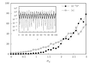
Figure 4: Analysis of the spatial coherence for the choice: $a=2$, $b=1$, $w=4$ $D=0.1$ and $\sigma_{\xi}=0$ (under the Stratonovich prescription). The intensity of the dominant mode was scaled by a factor $10^{-3}$ just to use the same axis scale. In the inset we exhibit typical patterns for low (solid line) and high (dotted line) noise intensities, namely for $\sigma_{\eta}=$ 0.1 and 1.9, respectively. The dotted lines are guides to the eyes.

One can cast a Stratonovich stochastic differential equation into the form of an Itô equation with an effective (or spurious) drift. For our Eq. (2), this implies the change $a\to a+\frac{K_{\eta}}{2}\sigma^{2}_{\eta}$. Because the additional term is positive, this change amounts to increasing the growth rate $a$. On the other hand, increasing $a$, with the other parameters fixed, does not alter the stability condition. This situation would lead to increase the average density and to strengthen patterns, which is in fact the outcome observed in Fig. 4, indicating that the destructive role observed for Itô noise (Fig. 3) is not enough to spoil the constructive effect of the spurious drift.

The effect of additive white noise when the multiplicative one is switched off ($\sigma_{\eta}=0$) is shown in Fig. 5. To ensure positiveness, negative fluctuations were trimmed, by setting $u(x,t+dt)=0$, if $u(x,t+dt)<0$. We did not apply any symmetrization procedure to keep the null mean value. Then truncations rise the noise mean value, producing a consequent shift of the population average. This effect becomes visible for large noise intensities, where the probability of trimming is not negligible.

Like multiplicative Itô fluctuations, additive noise also plays a destructive role in coherence, as can be observed in the decay of $S^{\star}$ with noise intensity. However, in this case, there is not an extinction threshold and the average density remains finite.

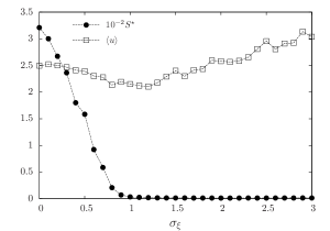
Figure 5: Analysis of the spatial coherence for $a=2$, $b=1$, $w=4$, $D=0.1$ and $\sigma_{\eta}=0$. The symbols correspond to numerical results. The dotted lines are guides to the eyes.

III.2 In the absence of deterministic patterns ($\lambda(k^{\star})<0$)

In this subsection we concentrate in our main case of interest, that is when the homogeneous solution is stable despite nonlocality. The purpose of analyzing this situation is to verify if the introduction of noise in the dynamic rules can inject coherence.

Let us first analyze the impact of the Itô multiplicative noise. In Fig. 6, we observe how the dominant mode intensity $S^{\star}$ changes as a function of the noise intensity $\sigma_{\eta}$. Our results point out that when noise intensity is small enough ($\sigma_{\eta}<1.0$), the increasing behavior $S^{\star}\propto\sigma_{\eta}^{2}$ predicted by Eq. (13) occurs. However, when we increase the noise intensity beyond the linear regime, we note that there is a break in the monotonic behavior of $S^{\star}$ with a peak that characterizes an optimum value $\sigma_{\eta}^{o}\approx 2.0$. Above this optimum value, noise starts to play a destructive role in spatial coherence. As a consequence, the dominant mode becomes less intense until it is completely destroyed. Actually, this is due to the concomitant decrease and extinction of the population, as shown by the quotient $S^{\star}/\langle u\rangle$ also exhibited in Fig. 6.

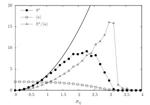
Figure 6: Analysis of the spatial coherence for $a=2$, $b=1$, $w=4$, $D=1$ and $\sigma_{\xi}=0$, for Itô noise. The symbols correspond to numerical results. The quotient $S^{\star}/\langle u\rangle$ is also plotted. The solid line corresponds to the theoretical prediction given by Eq. (13), the dotted lines are guides to the eyes.

On the one hand, noise in the reproduction rate affects the number of individuals in the population, as expected. Also in this case, there exists a value $\sigma_{\eta}^{c}\approx 3$ that represents the extinction threshold: if noise intensity exceeds that value, the population density vanishes, as discussed in Sec. III.1. On the other hand, although noise does not shift the dispersion relation, it forces an anticipation of mode instability, which is illustrated by the bursts of coherence displayed by density inhomogeneities in Fig. 7.

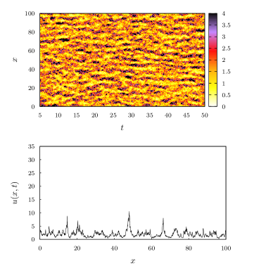
Figure 7: (Color online) Time evolution of the density $u(x,t)$ in a color map (upper panel), for $a=2$, $b=1$, $w=4$, $D=1$, $\sigma_{\xi}=0$, $\sigma_{\eta}=1.0$ (Itô noise). In the lower panel we exhibit a density profile corresponding to a cut of the color map at $t=50$.

Now we perform the same analysis for the Stratonovich case. Figure 8 displays the analysis of spatial coherence, while the time evolution is depicted in Fig. 9. In the inset of the last figure we also show the theoretical prediction given by Eq. (13), which is only valid up to a critical value, $\sigma_{\eta}^{c}\simeq 0.33$ in the case of the figure, point at which the theoretical structure function becomes divergent, although its numerical computation is possible.

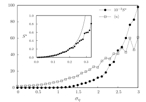
Figure 8: Analysis of the spatial coherence for $a=2$, $b=1$, $w=4$, $D=1$ and $\sigma_{\xi}=0$, for Stratonovich noise. The symbols correspond to numerical results. The inset shows a blow up of the vicinity of the origin, where the solid line corresponds to the theoretical prediction given by Eq. (13).

In terms of a spurious drift, Stratonovich noise would essentially lead to a larger growth rate, with the concomitant increase of the average density. Moreover, that spurious drift has the effect of shifting the dispersion relation, yielding Eq. (12). But, in contrast to Sec. III.1, increasing noise intensity can shift the maximum of the dispersion curve from the stability to the instability region for sufficiently large noise intensity (above its critical value). When this happens, differently to the Itô case for the same value of the parameters, persistence of spatial patterns emerges. The resulting profiles are similar to those observed for the parameter region in which patterns already occur in the deterministic limit.

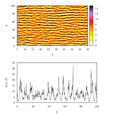
Figure 9: (Color online) Time evolution of the density $u(x,t)$ in a color map (upper panel), for $a=2$, $b=1$, $w=4$, $D=1$, $\sigma_{\xi}=0$ and $\sigma_{\eta}=1.0$ (Stratonovich case). In the lower panel we exhibit a profile corresponding to a cut of the color map at $t=50$.

Although for both noises one has $S^{\star}>0$, indicating the presence of coherence, in the Stratonovich case, $\Lambda_{1}(k^{\star})>0$ while in the Itô case $\Lambda_{0}(k^{\star})=\lambda(k^{\star})<0$. That is, despite some kind of coherence is always revealed by noise, in the Stratonovich case there is persistence of the patterns, while in the Itô case they are weakly correlated in time. Moreover, comparison of the profiles shown in Figs. (7) and (9), reveals a greater regularity and more pronounced peaks in the distribution $u(x,t)$ in the Stratonovich case.

In order to quantify the degree of persistence, we measured the spatial average of the time autocorrelation function of $u(x,t)$, $R(\tau)$ as a function of the time lag $\tau$. The autocorrelation function presents an exponential behavior after an abrupt decay, then, we considered different effective correlation times (as defined in Fig. 10), as measures of the degree of persistence. All these quantities plotted as a function of $\sigma_{\eta}$, under the Stratonovich interpretation, are presented in Fig. 10. The figure shows that persistence first increases with noise intensity, attaining a maximum, and thereafter decays with larger noise intensities for which order is spoiled. Notice than in the limit of vanishing noise intensity, the correlation times do not go to zero. The limiting values remain almost constant up to a value of $\sigma_{\eta}$ that approximately coincides with the critical one predicted by the condition $\Lambda_{1}(k^{\star})=0$ in Eq. (12). In the case of the figure, the aforementioned critical value is $\sigma_{\eta}^{c}\simeq 0.33$. In fact, the kind of persistence observed in Fig. 9 can be attributed to a positive maximum of the dispersion relation ($\Lambda_{\nu}(k^{\star})>0$). This condition is possible only for $\nu=1$ (Stratonovich interpretation) and $\sigma_{\eta}>\sigma_{\eta}^{c}$. Notice that, under the Itô interpretation ($\nu=0$), $\Lambda_{0}(k^{\star})$ is always negative if $\lambda(k^{\star})<0$, then such kind of persistent pattern cannot occur. In fact, for the Itô simulations, we observed (not shown) that below the extinction threshold noise does not affect the correlation times that remain at the level of those at vanishing noise intensity in the Stratonovich case. Hence we can conclude that for the same parameters, the effect of Itô noise is equivalent to that of Stratonovich noise below $\sigma_{\eta}^{c}$.

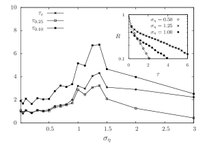
Figure 10: Correlation times as a function of $\sigma_{\eta}$, for $a=2$, $b=1$, $w=4$, $D=1$, $\sigma_{\xi}=0$ (with Stratonovich noise). The inset shows typical curves of the autocorrelation function vs the time lag $\tau$, from which correlation times were extracted: $\tau_{c}$ is the inverse rate of exponential decay, since there is an abrupt decay before the exponential regime, we also computed $\tau_{0.25}=\tau(R=0.25)$ and $\tau_{0.10}=\tau(R=0.10)$.

The impact of additive noise is shown in Fig. 11, confirming the possibility of induced coherence in this case, as predicted by Eq. (13). However, patterns present low temporal correlation, similarly to those in Fig. 7 for Itô fluctuations. Notice that Eq. (13) furnishes a good prediction of the impact of additive fluctuations observed in numerical simulations. This is because in the low noise intensity limit where Eq. (13) holds, the necessity of applying the truncation rule seldom occurs.

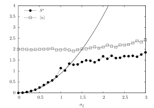
Figure 11: Analysis of the spatial coherence for $a=2$, $b=1$, $w=4$, $D=1$ and $\sigma_{\eta}=0$. The symbols correspond to numerical results. The solid line corresponds to the theoretical prediction given by Eq. (13), the dotted lines are guides to the eyes.

IV Final remarks

We incorporated stochasticity in a generalized Fisher-KPP equation, namely by adding noise to a characteristic parameter, the growth rate, as well as by means of an additive noise term. Then, we focused on the impact of such fluctuations on the stability of the asymptotic state. Although there is a formal correspondence between the Itô and Stratonovich rules to interpret multiplicative stochastic equations, we chose to present a parallel between them, for the same set of parameters, as soon as they apply to different scenarios of environment fluctuations.

When patterns are deterministically induced, Itô noise in parameter $a$ has a destructive role. Instead, when the homogeneous state is stable, noise destabilizes it, inducing the emergence of potentially dominant modes, which are hidden in the noiseless limit. However, extreme values of the noise intensity lead to extinction in both cases.

On the other side, when noise is interpreted in the Stratonovich sense, multiplicative fluctuations are able to increase population size as well as coherence, be patterns deterministically induced or not. Moreover, a crucial difference, noticed from numerical simulations, is the persistence of spatial patterns in the Stratonovich case, which is absent in the Itô one. We characterized the changes of persistence as a function of the intensity of Stratonovich noise, by directly measuring the temporal autocorrelation.

When patterns are deterministic, additive noise ($\sigma_{\xi}>0$) plays a destructive role in coherence. $S^{\star}$ decays with noise intensity, similarly to the scenario observed for Itô multiplicative fluctuations, but there is not an extinction threshold. In the absence of deterministic patterns, additive noise induces coherence, although with low temporal correlation, also as in the case of Itô fluctuations.

Future perspectives would be to consider fluctuations in the other parameters and to assume that noises possess characteristic finite scales, typical of natural environments.

References

- Malthus (1993) T. Malthus, An Essay on the Principle of Population, Oxford World’s Classics (Oxford University Press, UK, 1993).
- Verhulst (1838) P. F. Verhulst, Correspondance mathématique et physique 10, 113 (1838).
- Theraulaz et al. (2002) G. Theraulaz, E. Bonabeau, S. C. Nicolis, R. V. Solé, V. Fourcassié, S. Blanco, R. Fournier, J.-L. Joly, P. Fernández, A. Grimal, P. Dalle, and J.-L. Deneubourg, Proceedings of the National Academy of Sciences 99, 9645 (2002).
- Toner and Tu (1995) J. Toner and Y. Tu, Phys. Rev. Lett. 75, 4326 (1995).
- Rudge et al. (2013) T. J. Rudge, F. Federici, P. J. Steiner, A. Kan, and J. Haseloff, ACS Synthetic Biology 2, 705 (2013).
- Alim et al. (2013) K. Alim, G. Amselem, F. Peaudecerf, M. P. Brenner, and A. Pringle, Proceedings of the National Academy of Sciences 110, 13306 (2013).
- Castellano et al. (2009) C. Castellano, S. Fortunato, and V. Loreto, Rev. Mod. Phys. 81, 591 (2009).
- Murray (2002) J. D. Murray, Mathematical Biology: I. An Introduction, Interdisciplinary Applied Mathematics (Springer, 2002).
- Fuentes et al. (2004) M. A. Fuentes, M. N. Kuperman, and V. M. Kenkre, The Journal of Physical Chemistry B 108, 10505 (2004).
- Fuentes et al. (2003) M. A. Fuentes, M. N. Kuperman, and V. M. Kenkre, Physical Review Letters 91, 158104 (2003).
- da Cunha et al. (2011) J. A. R. da Cunha, A. L. A. Penna, and F. A. Oliveira, Physical Review E 83, 15201 (2011).
- Clerc et al. (2010) M. G. Clerc, D. Escaff, and V. M. Kenkre, Phys. Rev. E 82, 036210 (2010).
- Stephens and Sutherland (1999) P. A. Stephens and W. J. Sutherland, Trends in Ecology & Evolution 14, 401 (1999).
- Ratkowsky et al. (1982) D. A. Ratkowsky, J. Olley, T. A. McMeekin, and A. Ball, J. Bacteriol. 149, 1 (1982).
- Farrell and Rose (1967) J. Farrell and A. Rose, Annual Reviews in Microbiology 21, 101 (1967).
- Kolmogorov et al. (1937) A. N. Kolmogorov, I. G. Petrovskii, and N. S. Piskunov, Bjul. Moskovskogo Gos. Univ 1, 1 (1937).
- Fisher (1937) R. Fisher, Annals of Eugenics 7, 355 (1937).
- Murray (2003) J. D. Murray, Mathematical Biology II: Spatial Models and Biomedical Applications, Interdisciplinary Applied Mathematics (Springer, 2003).
- Kampen (1981) N. Kampen, Journal of Statistical Physics 24, 175 (1981).
- Turelli (1977) M. Turelli, Theoretical Population Biology 12, 140 (1977).
- Lande (1993) R. Lande, American Naturalist , 911 (1993).
- Sagués et al. (2007) F. Sagués, J. Sancho, and J. García-Ojalvo, Reviews of Modern Physics 79, 829 (2007).
- Agez et al. (2013) G. Agez, M. G. Clerc, E. Louvergneaux, and R. G. Rojas, Phys. Rev. E 87, 042919 (2013).
- Ridolfi et al. (2011) L. Ridolfi, P. D’Odorico, and F. Laio, Noise-induced phenomena in the environmental sciences (Cambridge University Press, 2011).
- Cross and Hohenberg (1993) M. Cross and P. Hohenberg, Reviews of Modern Physics 65, 851 (1993).
- Colombo and Anteneodo (2012) E. H. Colombo and C. Anteneodo, Physical Review E 86, 36215 (2012).
- Ibañes et al. (2000) M. Ibañes, J. García-Ojalvo, R. Toral, and J. M. Sancho, in Stochastic Processes in Physics, Chemistry, and Biology (Springer, 2000) pp. 247–256.
- Novikov (1965) E. A. Novikov, JETP 20, 1290 (1965).
- Schöpf and Zimmermann (1993) W. Schöpf and W. Zimmermann, Physical Review E 47, 1739 (1993).
- Carrillo et al. (2004) O. Carrillo, M. A. Santos, J. García-Ojalvo, and J. M. Sancho, EPL (Europhysics Letters) 65, 452 (2004).
- Horsthemke and Lefever (2006) W. Horsthemke and R. Lefever, Noise-Induced Transitions: Theory and Applications in Physics, Chemistry, and Biology, Springer complexity (Physica-Verlag, 2006).