Spin-Valley Filtering in Strained Graphene Structures with Artificially Induced Carrier Mass and Spin-Orbit Coupling

Abstract

The interplay of massive electrons with spin-orbit coupling in bulk graphene results in a spin-valley dependent gap. Thus, a barrier with such properties can act as a filter, transmitting only opposite spins from opposite valleys. In this Letter we show that a strain induced pseudomagnetic field in such a barrier will enforce opposite cyclotron trajectories for the filtered valleys, leading to their spatial separation. Since spin is coupled to the valley in the filtered states, this also leads to spin separation, demonstrating a spin-valley filtering effect. The filtering behavior is found to be controllable by electrical gating as well as by strain.

Graphene is considered a promising material for future spintronic applications, in part due to its long spin relaxation length pesin12 ; tomb07 ; zomer12 . Furthermore, owing to its band structure with two inequivalent valleys, $K$ and $K^{\prime}$, it has revived the field of valleytronics rycerz07 ; neto09 . The low energy excitations in the two valleys behave as Dirac-Weyl particles, which is most famously manifested in the presence of a magnetic field, in which Landau levels scale as $\sqrt{B}$, with a unique level at zero energy neto09 ; grujic11 . Besides, it is known that straining graphene causes time-reversal invariant gauge fields to appear, i.e., an effective magnetic field with opposite signs in opposite valleys, providing a tool for manipulating the valley degree of freedom neto09 . Recent experiments demonstrated large values of this pseudomagnetic field, which could hardly be matched in practical applications by real magnetic fields levy10 .

In this Letter we study the transmission through a thin 1D graphene barrier with artificially induced mass and spin-orbit coupling (SOC), in the presence of a pseudomagnetic field using the continuum approach. Our motivation for studying such a structure is twofold. In part it is due to a shift to a new paradigm in 2D materials research, whereby their properties are custom tailored according to specific needs by stacking different 2D crystals on top of each other. These are the so-called van der Waals heterostructures geim13 . More importantly, and in the light of this paradigm, recent theoretical and experimental work suggests that mass and SOC, which are vanishing in intrinsic graphene, could be induced with appropriate substrates and/or adatom deposition zhong11 ; sachs11 ; kinder12 ; amet13 ; hunt13 ; neto2009 ; weeks11 ; alicea12 ; ozy13 ; jin13 ; ozy14 . The studied device is found to behave as a spin-valley filter, thus lying in the intersection of the fields of spintronics and valleytronics.

In the continuum approach the carrier mass is captured by a staggered potential term $\Delta$, while SOC is captured by a masslike term $\Delta_{SO}$. The presence of both will result in a competition to open topologically distinct gaps kane05 . This competition reflects on the gap size given by $2\left|s\tau\Delta_{SO}+\Delta\right|$, where $s=+1/-1$ labels the spin $\uparrow/\downarrow$ and $\tau=+1/-1$ labels the valley $K/K^{\prime}$ degrees of freedom ezawa13 . Thus, for different spin-valleys different gaps can arise. In order to get some insight into the problem, we first study transmission through a barrier with a real magnetic field. Regardless of the magnetic field, whenever $\Delta_{SO}\neq 0$ and $\Delta\neq 0$, there is an energy range where $s\tau=+1$ states are suppressed, while $s\tau=-1$ states are not. In other words only one spin from one valley, and the opposite spin from the opposite valley are transmitted. The main effect of the magnetic field is to impose restrictions on incident angles over which the transmission can occur. This is caused by the cyclotron orbits, which are the same for all spins and valleys.

We subsequently apply the pseudomagnetic field, which leads to the reversal of the effective field, and the effective cyclotron orbits in one of the valleys. This provides the benefit of spatially separating the transmitted states according to their valley degree of freedom, and accordingly their spin degree of freedom as well. Thus a combined spin-valley filter can be obtained. Furthermore, we show that chemical potential and strain can act as a switch, rendering control over the filtering behavior. Filtering behavior in graphene devices was studied before chaves10 ; masir11 ; wu11 ; dean12 ; jiang13 ; myoung13 ; tsai13 ; lu13 ; yoko13 ; yoko14 ; however the mechanism proposed in this Letter is novel, and previously unexplored. Practical implications are discussed at the end of the Letter.

Our starting point is the Dirac-Weyl equation, in the presence of mass, SOC, and a magnetic field perpendicular to the sheet, $B_{z}$. In this case we choose the Landau gauge $\mathbf{A}=\left(0,A_{y}\right)$, and the Dirac-Weyl Hamiltonian reads

$$H=\hbar v_{F}\left[\tau k_{x}\sigma_{x}+(k_{y}+\frac{e}{\hbar}A_{y})\sigma_{y}\right]+s\tau\Delta_{SO}\sigma_{z}+\Delta\sigma_{z},$$ (1)

where $v_{F}$ is the Fermi velocity, and $\sigma_{z}$ is a Pauli matrix operating in the sublattice subspace.

We use the parameter $\tau_{B}$, such that $B_{z}=\tau_{B}B$, to capture the valley-dependent nature of the pseudomagnetic field. Setting $\tau_{B}=+1$ models the influence of the real magnetic field, while $\tau_{B}=\pm\tau$ models the two types of the pseudomagnetic field. The (pseudo)magnetic field, mass, and SOC exist only in the barrier of width $W$. The vector potential is therefore given by

$$A_{y}=\begin{cases}0,&x<0\\ \tau_{B}Bx,&0\leq x\leq W\\ \tau_{B}BW,&x>W\end{cases}.$$ (2)

In the chosen Landau gauge $k_{y}$ is a good quantum number and the solutions have the form $\Psi(x,y)=\exp(ik_{y}y)\left(\psi_{A}(x),\psi_{B}(x)\right)^{T}$. Introducing $\hbar v_{F}\epsilon=E$, and $\hbar v_{F}\delta=s\tau\Delta_{SO}+\Delta$, and decoupling the system, in the barrier one obtains

$$\left[\partial_{x}^{2}\mp\tau\tau_{B}\frac{1}{l_{B}^{2}}-(k_{y}+\tau_{B}\frac{x}{l_{B}^{2}})^{2}+\epsilon^{2}-\delta^{2}\right]\psi_{A/B}=0,$$ (3)

where $l_{B}=\sqrt{\hbar/eB}$. Using the transformation $z=\sqrt{2}\left(k_{y}l_{B}+\tau_{B}x/l_{B}\right)$, the solutions are expressed in terms of the parabolic cylinder functions $D_{\nu}(z)$ (see the Supplemental Material supmat for details), and read

$$\psi_{II}=C_{1}\left(\begin{array}[]{c}D_{\nu_{A}}(z)\\ gD_{\nu_{B}}(z)\end{array}\right)+C_{2}\left(\begin{array}[]{c}D_{\nu_{A}}(-z)\\ -gD_{\nu_{B}}(-z)\end{array}\right),$$ (4)

where $\nu_{A/B}=\left(\epsilon^{2}-\delta^{2}\right)l_{B}^{2}/2\mp\tau\tau_{B}/2-1/2$, and

$$g=i\left[\frac{\sqrt{2}}{\left(\epsilon+\tau\tau_{B}\delta\right)l_{B}}\right]^{\tau\tau_{B}}.$$ (5)

On the other hand, the incident wave function is

$$\psi_{I}=e^{ik_{x}x}\left(\begin{array}[]{c}1\\ \tau e^{i\tau\phi}\end{array}\right)+re^{-ik_{x}x}\left(\begin{array}[]{c}1\\ \tau e^{i\tau(\pi-\phi)}\end{array}\right),$$ (6)

while the solution in the third region reads

$$\psi_{III}=t\sqrt{\frac{k_{x}}{k_{x}^{\prime}}}e^{ik_{x}^{\prime}x}\left(\begin{array}[]{c}1\\ \tau e^{i\tau\theta}\end{array}\right).$$ (7)

Here, $\phi=\arctan k_{y}/k_{x}$ and $\theta=\arctan k_{y}^{\prime}/k_{x}^{\prime}$ denote the energy propagation directions before and after the barrier, where $k_{y}=q_{y}\left(0\right)$ and $k_{y}^{\prime}=q_{y}\left(W\right)$, while $q_{y}\left(x\right)=\epsilon\sin\phi+eA_{y}\left(x\right)/\hbar$ is the effective transverse momentum. The longitudinal momenta before and after the barrier are given by $k_{x}=\epsilon\cos\phi$ and $k_{x}^{\prime}=\epsilon\cos\theta$ supmat . Note that all these expressions are valid for the valence band as well supmat . Matching the wave functions at the interfaces gives a system of equations, whose solution yields the transmission amplitude $t$

$$t=\frac{2g\tau\cos\phi\left(G_{A}^{+}G_{B}^{-}+G_{A}^{-}G_{B}^{+}\right)}{e^{ik_{x}^{\prime}W}f}\sqrt{\frac{k_{x}^{\prime}}{k_{x}}},$$ (8)

where

$$\begin{split}f=g^{2}\left(F_{B}^{+}G_{B}^{-}-F_{B}^{-}G_{B}^{+}\right)+e^{i\tau\left(\theta-\phi\right)}\left(F_{A}^{+}G_{A}^{-}-F_{A}^{-}G_{A}^{+}\right)\\ +g\tau e^{i\tau\theta}\left(F_{B}^{-}G_{A}^{+}+F_{B}^{+}G_{A}^{-}\right)+g\tau e^{-i\tau\phi}\left(F_{A}^{+}G_{B}^{-}+F_{A}^{-}G_{B}^{+}\right).\end{split}$$ (9)

Here the coefficients $F^{\pm}$ and $G^{\pm}$ are given by

$$F^{\pm}_{A/B} =D_{\nu_{A/B}}\left[\pm\sqrt{2}k_{y}l_{B}\right],$$ (10)

$$G^{\pm}_{A/B} =D_{\nu_{A/B}}\left[\pm\sqrt{2}\left(k_{y}l_{B}+\tau_{B}\frac{W}{l_{B}}\right)\right].$$ (11)

In Fig. 1 we look at the behavior of transmission coefficients ($T=\left|t\right|^{2}$) in detail for a real magnetic field ($\tau_{B}=+1$). Here we show contour plots of, from top to bottom, $T_{\uparrow K}$, $T_{\uparrow K^{\prime}}$, $T_{\downarrow K}$ and $T_{\downarrow K^{\prime}}$, as a function of incident energy and angle. We adopt a set of parameters that illustrates our main points clearly: $\Delta_{SO}=30$ meV, $W=100$ nm and $B=0.2$ T, whereas $\Delta$ varies from $0$ in (a), to $\Delta=15$ meV in (b) and $\Delta=30$ meV in (c).

A common feature of all the cases depicted in Fig. 1 is that transmission is forbidden outside the transmission window delineated by the solid black line. This is because the magnetic field enforces cyclotron motion, resulting in asymmetric transmission curves with respect to the incidence angle martino07 ; masir08 . This boundary is obtained by requiring that the longitudinal momentum after the barrier becomes imaginary, so that only evanescent waves can exit, and therefore no transmission can occur. The longitudinal momentum in the third region is given by $k_{x}^{\prime 2}=\epsilon^{2}-q_{y}\left(W\right)^{2}$. Hence, this window is determined by a critical energy, below (above) which the transmission is not possible

$$\epsilon_{cr1}^{c/v}=\frac{\pm\gamma}{1\mp\tau_{B}\sin\phi},$$ (12)

where $\gamma=W/l_{B}^{2}$, and $c$ ($v$) denotes the conduction (valence) band. The window depends on $W,B$ and $\phi$, i.e., it is not a function of $\Delta_{SO},\Delta,s$ or $\tau$ at all, as can be observed in Fig. 1. However, the transmission within this window obviously depends on $\Delta_{SO},\Delta,s$ and $\tau$.

As already mentioned, in the presence of mass and SOC, the bulk band gap is given by $2\left|s\tau\Delta_{SO}+\Delta\right|$. Therefore, when both parameters are present, the $s\tau=+1$ states experience a larger gap than the $s\tau=-1$ states. To see how this might reflect on the transmission through a barrier we need to examine the behavior of the quasiclassical momentum within the barrier $q_{x}\left(x\right)=\sqrt{\epsilon^{2}-\delta^{2}-q_{y}\left(x\right)^{2}}$ supmat . Therefore, through the appearance of $\delta$, the quasiclassical momentum depends on $\Delta_{SO},\Delta,s$ and $\tau$. More specifically, when both $\Delta$ and $\Delta_{SO}$ are nonzero, whether classically forbidden regions inside the barrier will appear depends crucially on the product $s\tau$, which is a clear manifestation of the bulk band gap. The existence of forbidden regions in the barrier does not necessarily imply that the momentum after the barrier is imaginary. To see this, one can express the critical energy below (above) which the former happens

$$\epsilon_{cr2}^{c/v}=\pm\max\left(\frac{\pm\tau_{B}\gamma\sin\phi+\sqrt{\gamma^{2}+\delta^{2}\cos^{2}\phi}}{\cos^{2}\phi},\frac{\left|\delta\right|}{\cos\phi}\right).$$ (13)

This critical boundary is drawn in dashed black lines in Fig. 1, and it coincides with the transmission window (Eq. (12)) only when the bulk band gap is closed. Therefore, in between $\epsilon_{cr1}^{c}$ and $\epsilon_{cr2}^{c}$ transmission is possible, but only by tunneling through the forbidden region (regions) in the barrier, and thus perfect transmission cannot occur. Above the $\epsilon_{cr2}^{c}$ boundary, however, there is no attenuation within the barrier, and the resulting transmission is determined by the interference of electron waves. It is important to point out that below the minimum of $\epsilon_{cr2}^{c}$, which coincides with the bottom of the conduction band, the transmission is strongly suppressed.

One issue requires clarification. For the case $\Delta=0$, shown in Fig. 1(a), $\epsilon_{cr2}^{c}$ is the same for all spin and valley flavors. However, the transmissions for spin up and spin down are obviously different. This discrepancy arises due to the factor $g$, appearing in the transmission amplitude, Eq. (8). This factor is in turn just a reflection of the form of the Landau level (LL) eigenstates supmat . In fact one can easily show that the solution given by Eq. (4) reduces to the LL eigenstates once the incident energy is equal to a particular LL supmat .

It is known that inversion symmetry breaking can lead to the appearance of magnetic moments coupled with the valley degree of freedom, which in turn influence the LLs xiao07 . Similar moments arise when SOC is present as well, albeit coupled with the spin degree of freedom supmat . It is these moments that cause spin-distinguished transmission found in Fig. 1(a). A similar behavior occurs when only $\Delta$ is nonzero, but with valley differentiation instead. In fact, we have found that all of the contour plots obey the symmetry $\Delta_{SO}\leftrightarrow\Delta$, $s\leftrightarrow\tau$. This stems from the fact that the band gap and the magnetic moments display the same symmetry as well supmat . We stress, however, that this behavior has little to no impact on the effect we describe here, and will be studied in detail elsewhere.

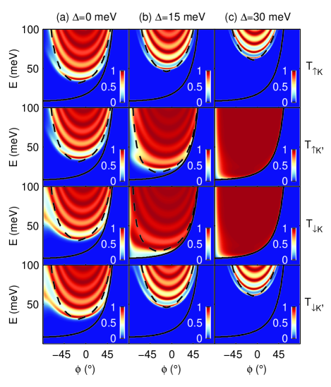
Figure 1: Contour plots of transmission coefficient versus energy and incident angle, for all spin and valley flavors. $\Delta_{SO}$ equals $30$ meV, while $\Delta$ is varied: (a) $\Delta=0$, (b) $\Delta=15$ meV and (c) $\Delta=30$ meV. The width of the barrier is taken to be $W=100$ nm, and $B=0.2$ T.

Introducing $\Delta$ will cause shrinking (enlarging) of the evanescent region for $s\tau=-1$ ($s\tau=+1$), Fig. 1(b). This will lead to the appearance of an energy range where only $s\tau=-1$ states are not suppressed. Furthermore note that these states also display lower fringe constrast. This is because the barrier is effectively reduced for these states. Finally, for the case $\Delta_{SO}=\Delta$, depicted in column (c), $s\tau=+1$ states are even further suppressed. On the other hand, for $s\tau=-1$ the barrier vanishes, as the effective dispersion returns to a Dirac cone. These states are influenced only by the magnetic field martino07 ; masir08 , which can also be inferred from the fact that now $\epsilon_{cr1}^{c/v}=\epsilon_{cr2}^{c/v}$. This means that they experience no reflection at the walls of the barrier and as a consequence there are no resonances.

Therefore, as long as $\Delta_{SO}\neq 0$ and $\Delta\neq 0$, in a particular energy range only spin up states from the $K$ valley and spin down states from the $K^{\prime}$ valley are transmitted. Introducing a pseudomagnetic field, by for instance setting $\tau_{B}=+\tau$, means that the effective magnetic field in $K^{\prime}$ valley flips. This in turn flips the transmission window in this valley to $\epsilon_{cr1K^{\prime}}^{c}=\gamma/\left(1+\sin\phi\right)$. Thus, spatial separation of the states from each valley will occur, which is an obvious consequence of their opposite cyclotron trajectories. Furthermore, since spin is coupled to the valley degree of freedom in the transmitted states, this will inevitably lead to spin separation as well.

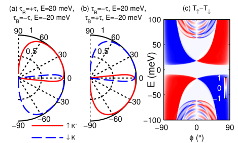
Figure 2: Polar plots of the transmission coefficient versus the incident angle for various strains and energies. In (a) $\tau_{B}=\pm\tau$, $E=\pm 20$ meV give the same transmission, while in (b) $\tau_{B}=\mp\tau$, $E=\pm 20$ meV give the same transmission. All other parameters are the same as in Fig. 1(c). The electric control of the spin-valley filtering is clearly seen in (c), where the contour plot of $T_{\uparrow}-T_{\downarrow}$ is shown.

Additionally, it follows from Eq. (8) that the transmission coefficient for $-\phi$, $-s$, $-\tau$ equals the one for $\phi$, $s$, $\tau$, which is a manifestation of time-reversal symmetry footnote1 . In other words, the transmission for spins in the valley where the effective magnetic field is reversed, will just be a mirror image of the transmission from the opposite valley and opposite spin, for which the effective magnetic field stayed the same. This is displayed in Fig. 2(a), for the same set of parameters as in Fig. 1(c), and $E=20$ meV, where the spin-valley filtering behavior is apparent. On the other hand, by choosing the opposite strain, $\tau_{B}=-\tau$, the effective magnetic field will be flipped in both valleys. This will lead to flipping of the filtered spin and valley, as depicted in Fig. 2(b), since both transmission windows flip (see Eq. (12)). In other words strain could act as a switch footnote2 .

Furthermore, the switching can also be achieved by controlling the chemical potential instead of strain. To see this, note that the transmission window for a given spin and valley in the valence band $\epsilon_{cr1}^{v}$ is a mirror reverse of the one in the conduction band $\epsilon_{cr1}^{c}$, Eq. (12). This is a consequence of different cyclotron trajectories for electrons and holes, and the same symmetry is obeyed by the semiclassical critical boundary, given in Eq. (13). Moreover, since $T\left(\epsilon,\tau_{B}=+\tau\right)=T\left(-\epsilon,\tau_{B}=-\tau\right)$ holds, Figs. 2(a) and (b) also correspond to $\tau_{B}=-\tau$, $E=-20$ meV and $\tau_{B}=\tau$, $E=-20$ meV, respectively supmat . The effect of controlling the chemical potential on spin filtering is depicted in Fig. 2(c), where the outlines of the transmission windows can be clearly seen. Note that the same plot holds for $T_{K^{\prime}}-T_{K}$, albeit with opposite filtering in the overlap region of both transmission windows. Therefore, the control of the transmitted spin-valley outside of the transmissionless gap $\left[-\gamma/2,\gamma/2\right]$ could be established by means of electrical gating. Additionally, there exist optimal energy ranges for filtering in the valence and conduction band, $\left[-\gamma,-\gamma/2\right]$ and $\left[\gamma/2,\gamma\right]$, respectively, where the transmitted states do not overlap supmat .

Finally, we include some practical considerations. First note that only minor straining would be required for inducing a pseudomagnetic field of $0.2$ T in a $100$ nm wide barrier, given the strain pattern described in Ref. guinea10 . Since $\Delta_{SO}$ and $\Delta$ equal zero in graphene, these two parameters would have to be induced artificially in the barrier, a feat possible because bulk electrons are fully exposed on the graphene surface. Hexagonal boron nitride (hBN) has an intrinsically broken inversion symmetry, and forms a generally higher quality electronic heterostructure with graphene as opposed to other substrates dean10 , manifested in reduced charge impurities, ultraflatness, and high electron mobility. It also has a minuscule lattice mismatch with respect to graphene zhong11 , which causes a moiré pattern, resulting in a Hofstadter fractal spectrum ponomarenko13 ; dean13 . While the emerging superlattice potential was suggested to induce insulating puddles with opposing masses sachs11 ; zarenia12 , it was also argued that an average gap should be opened nevertheless kinder12 . Recently, a gap of about $30$ meV in a graphene/hBN composite, consistent with inversion symmetry breaking was detected hunt13 ; woods14 . The average gap appears because the area of the favored commensurate stacking expands by stretching of the graphene lattice, once the two layers are well aligned amet13 ; woods14 ; jung14 .

On the other hand, it was suggested that engineering SOC in graphene can be achieved by adatoms or substrates neto2009 ; weeks11 ; alicea12 ; jin13 . This was indeed experimentally verified recently, where SOC as high as $17$ meV was observed ozy13 ; ozy14 . Since SOC in Eq. (1) commutes with out-of-plane spin, increasing it will not affect scattering of this spin component. However, inversion symmetry breaking will cause new extrinsic spin relaxation mechanisms pesin12 ; ochoa12 . The use of hBN as a substrate would prove beneficial here, since it was shown that the resulting heterostructure supports very long spin relaxation lengths zomer12 . Moreover, we argue that scattering processes could also be reasonably reduced by manipulating barrier length and/or strain patterns.

In conclusion, we proposed a device that enables filtering and spatial separation of opposite spin-valley pairs. The proposed spin-valley filter consists of a strained barrier with artificially engineered electron mass and SOC. Nanoribbon geometry could provide the practical testing ground for this effect, with the barrier formed perpendicular to the ribbon. If $\Delta>\Delta_{SO}$, the device would be in the topologically trivial phase, and the polarized current could in principle be detected by leads attached to the edges of the ribbon. On the other hand, if $\Delta_{SO}>\Delta$, edge states could become a nuisance. However the device could still operate in the domain of electron optics. In other words, the effect would be observable for a sufficiently collimated beam injected far from the edges. Collimation could also be achieved by means of a smooth Klein barrier in front of the studied device che06 .

- (1) Dmytro Pesin and Allan H. MacDonald, Nat. Mater. 11, 409 (2012).
- (2) Nikolaos Tombros, Csaba Jozsa, Mihaita Popinciuc, Harry T. Jonkman, and Bart J. van Wees, Nature (London) 448, 571 (2007).
- (3) P. J. Zomer, M. H. D. Guimarães, N. Tombros, and B. J. van Wees, Phys. Rev. B 86, 161416 (2012).
- (4) A. Rycerz, J. Tworzydło, and C. W. J. Beenakker, Nat. Phys. 3, 172 (2007).
- (5) A. H. Castro Neto, F. Guinea, N. M. R. Peres, K. S. Novoselov, and A. K. Geim, Rev. Mod. Phys. 81, 109 (2009).
- (6) M. Grujić, M. Zarenia, A. Chaves, M. Tadić, G. A. Farias, and F. M. Peeters, Phys. Rev. B 84, 205441 (2011).
- (7) N. Levy, S. A. Burke, K. L. Meaker, M. Panlasigui, A. Zettl, F. Guinea, A. H. Castro Neto, and M. F. Crommie, Science 329, 544 (2010).
- (8) A. K. Geim and I. V. Gregorieva, Nature (London) 499, 419 (2013).
- (9) Xiaoliang Zhong, Yoke Khin Yap, Ravindra Pandey, and Shashi P Karna, Phys. Rev. B 83, 193403 (2011).
- (10) B. Sachs, T. O. Wehling, M. I. Katsnelson, and A. I. Lichtenstein, Phys. Rev. B 84, 195414 (2011).
- (11) M. Kindermann, Bruno Uchoa, and D. L. Miller, Phys. Rev. B 86, 115415 (2012).
- (12) F. Amet, J. R. Williams, K. Watanabe, T. Taniguchi, and D. Goldhaber-Gordon, Phys. Rev. Lett. 110, 216601 (2013).
- (13) B. Hunt, J. D. Sanchez-Yamagishi, A. F. Young, M. Yankowitz, B. J. LeRoy, K. Watanabe, T. Taniguchi, P. Moon, M. Koshino, P. Jarillo-Herrero, and R. C. Ashoori, Science 340, 1427 (2013).
- (14) A. H. Castro Neto and F. Guinea, Phys. Rev. Lett. 103, 026804 (2009).
- (15) C. Weeks, J. Hu, J. Alicea, M. Franz, and R. Wu, Phys. Rev. X 1, 021001 (2011).
- (16) Jun Hu, Jason Alicea, Ruqian Wu, and Marcel Franz, Phys. Rev. Lett. 109, 266801 (2012).
- (17) J. Balakrishnan, G. K. Koon, M. Jaiswal, A. H. Castro Neto, and B. Özyilmaz, Nature Phys. 9, 284 (2013).
- (18) Kyung-Hwan Jin and Seung-Hoon Jhi, Phys. Rev. B 87, 075442 (2013).
- (19) Barbaros Özylmaz, in Scientific Workshop on 2D Materials: Beyond Graphene, Singapore, December 2013 (unpublished).
- (20) C. L. Kane and E. J. Mele, Phys. Rev. Lett. 95, 226801 (2005).
- (21) Motohiko Ezawa, Europhys. Lett. 104, 27006 (2013).
- (22) A. Chaves, L. Covaci, Kh. Yu. Rakhimov, G. A. Farias, and F. M. Peeters, Phys. Rev. B 82, 205430 (2010).
- (23) M. Ramezani Masir, A. Matulis, and F. M. Peeters, Phys. Rev. B 84, 245413 (2011).
- (24) Zhenhua Wu, F. Zhai, F. M. Peeters, H. Q. Xu, and Kai Chang, Phys. Rev. Lett. 106, 176802 (2011).
- (25) D. Moldovan, M. Ramezani Masir, L. Covaci, and F. M. Peeters, Phys. Rev. B 86, 115431 (2012).
- (26) Yongjin Jiang, Tony Low, Kai Chang, Mikhail I. Katsnelson, and Francisco Guinea, Phys. Rev. Lett. 110, 046601 (2013).
- (27) Nojoon Myoung and Gukhyung Ihm, arXiv:1312.2667v1.
- (28) Wei-Feng Tsai, Cheng-Yi Huang, Tay-Rong Chang, Hsin Lin, Horng-Tay Jeng, and A. Bansil, Nat. Commun. 4, 1500 (2013).
- (29) Wei-Tao Lu, Wen Li, Yong-Long Wang, Hua Jiang, and Chang-Tan Xu, Appl. Phys. Lett. 103, 062108 (2013).
- (30) T. Yokoyama, Phys. Rev. B 87, 241409 (2013).
- (31) Takehito Yokoyama, arXiv:1403.1962v2.
- (32) See Supplemental Material at http://link.aps.org/supplemental/10.1103/PhysRevLett.113.046601, which includes Refs. [31-34], for a detailed derivation.
- (33) P. E. Allain and J. N. Fuchs, Eur. Phys. J. B 83, 301 (2011).
- (34) Di Xiao, Wang Yao, and Qian Niu, Phys. Rev. Lett. 99, 236809 (2007).
- (35) Tianyi Cai, Shengyuan A. Yang, Xiao Li, Fan Zhang, Junren Shi, Wang Yao, and Qian Niu, Phys. Rev. B 88, 115140 (2013).
- (36) Mikito Koshino and Tsuneya Ando, Phys. Rev. B 81, 195431 (2010).
- (37) A. De Martino, L. Dell’Anna, and R. Egger, Phys. Rev. Lett. 98, 066802 (2007).
- (38) M. Ramezani Masir, P. Vasilopoulos, A. Matulis, and F. M. Peeters, Phys. Rev. B 77, 235443 (2008).
- (39) In supmat we demonstrate that , allowing a straightforward interpretation of Fig. 2 in terms of the exiting angle as well.
- (40) Note that the symmetry does not hold in general, due to the forementioned interplay with the orbital magnetic moments, although it effectively appears so.
- (41) F. Guinea, A. K. Geim, M. I. Katsnelson, and K. S. Novoselov, Phys. Rev. B 81, 035408 (2010).
- (42) C. R. Dean, A. F. Young, I. Meric, C. Lee, L. Wang, S. Sorgenfrei, K. Watanabe, T. Taniguchi, P. Kim, K. L. Shepard, and J. Hone, Nat. Nanotechnol. 5, 722 (2010).
- (43) L. A. Ponomarenko, R. V. Gorbachev, G. L. Yu, D. C. Elias, R. Jalil, A. A. Patel, A. Mishchenko, A. S. Mayorov, C. R.Woods, J. R. Wallbank, M. Mucha-Kruczynski, B. A. Piot, M. Potemski, I. V. Grigorieva, K. S. Novoselov, F. Guinea, V. I. Fal ko, and A. K. Geim, Nature 497, 594 (2013).
- (44) C. R. Dean, L. Wang, P. Maher, C. Forsythe, F. Ghahari, Y. Gao, J. Katoch, M. Ishigami, P. Moon, M. Koshino, T. Taniguchi, K. Watanabe, K. L. Shepard, J. Hone, and P. Kim, Nature (London) 497, 598 (2013).
- (45) M. Zarenia, O. Leenaerts, B. Partoens, and F. M. Peeters, Phys. Rev. B 86, 085451 (2012).
- (46) C. R.Woods, L. Britnell, A. Eckmann, R. S. Ma, J. C. Lu, H. M. Guo, X. Lin, G. L. Yu, Y. Cao, R. V. Gorbachev, A. V. Kretinin, J. Park, L. A. Ponomarenko, M. I. Katsnelson, Yu. N. Gornostyrev, K.Watanabe, T. Taniguchi, C. Casiraghi, H-J. Gao, A. K. Geim and K. S. Novoselov, Nat. Phys. 10, 451 (2014).
- (47) Jeil Jung, Ashley DaSilva, Shaffique Adam, and Allan H. MacDonald, arXiv:1403.0496v1.
- (48) H. Ochoa, A. H. Castro Neto, and F. Guinea, Phys. Rev. Lett. 108, 206808 (2012).
- (49) V. V. Cheianov and V. I. Fal’ko, Phys. Rev. B 74, 041403 (2006).