Parametric Strategy Iteration

Abstract

Program behavior may depend on parameters, which are either configured before compilation time, or provided at runtime, e.g., by sensors or other input devices. Parametric program analysis explores how different parameter settings may affect the program behavior.

In order to infer invariants depending on parameters, we introduce parametric strategy iteration. This algorithm determines the precise least solution of systems of integer equations depending on surplus parameters. Conceptually, our algorithm performs ordinary strategy iteration on the given integer system for all possible parameter settings in parallel. This is made possible by means of region trees to represent the occurring piecewise affine functions. We indicate that each required operation on these trees is polynomial-time if only constantly many parameters are involved.

Parametric strategy iteration for systems of integer equations allows to construct parametric integer interval analysis as well as parametric analysis of differences of integer variables. It thus provides a general technique to realize precise parametric program analysis if numerical properties of integer variables are of concern.

0.1 Introduction

Since the very beginnings of linear programming, parametric versions of linear programming (LP for short) have already been of interest (see, e.g., [6, 8] for an overview and [16] for recent algorithms). Parametric LP can be applied to answer questions such as: how much does the result of the analysis (optimal value/solution) depend on specific parameters? What is the precise dependency between a parameter and the result? In which regions of parameter values do these dependencies significantly change? Such types of sensitivity and mode analyses are important in order to obtain a better understanding of the problem under consideration and its potential analysis. Sensitivity and mode questions equally apply to programs whose behavior depends on parameters. Such parameters either could be provided at configuration time by engineers, or at runtime, e.g., through sensor data or other kinds of input. The goal then is to determine how the output values produced by the program may be influenced by the parameters. The same software may, e.g., control the break of a truck or a car, but must behave quite differently in the two use cases.

Here, we consider the static analysis of parameterized systems and propose methods for inferring, how numerical program invariants may depend on the parameters of the program. These questions cannot be answered by linear or integer linear programming related techniques alone, since the constraints to be solved are necessarily non-convex. Still, such questions can be answered for interval analysis or, more generally, for template-based numerical analyses such as difference bound matrices or octagons, since their analysis results can be expressed in first-order linear real arithmetic. This observation has been exploited by Monniaux [22] who applied quantifier elimination algorithms to obtain parametric analysis results. The resulting system can provide amazing results. However, if the programs under consideration have more complicated control-flow, i.e., do not consist of a single program point only, fixpoint computation realized by means of quantifier elimination does no longer seem appropriate.

In this paper, we are concerned with invariants over integers (opposed to rationals in Monniaux’ system).

Example 1.

Consider the following parametric program:

$$x={\bf p}_{1};\;{\bf while}\;(x<{\bf p}_{2})\;x=x+1;$$

where ${\bf p}_{1},{\bf p}_{2}$ are the parameters. The parametric invariant for program exit states that $x={\bf p}_{1}$ holds, if ${\bf p}_{2}\leq{\bf p}_{1}$, and $x={\bf p}_{2}$ otherwise. Thus, the analysis should distinguish two modes where the invariant inferred for program exit is significantly different, namely the set of parameter settings where ${\bf p}_{2}\leq{\bf p}_{1}$ holds and its complement. In the first mode, the value of $x$ at program exit is only sensitive to changes of the parameter ${\bf p}_{1}$, while otherwise it is sensitive to changes of the parameter ${\bf p}_{2}$.  

Note that for integer linear arithmetic, quantifier elimination is even more intricate than over the rationals. As shown in [9, 10, 11], non-parametric interval analysis as well as the analysis of differences of integer variables can be compiled into suitable integer equations. In absence of parameters, integer equation systems where no integer multiplication or division is involved, can be solved without resorting to heavy machinery such as integer linear programming. Instead, an iteration over max-strategies suffices [9, 10, 11]. Here, a max-strategy maps each application of a maximum operator to one of its arguments. Once a choice is made at each occurrence of a maximum operator, a conceptually simpler system is obtained. For systems without maximum operators, the greatest solution can be determined by means of a generalization of the Bellman-Ford algorithm. The greatest solutions of the maximum-free systems encountered during the iteration on max-strategies, provide us with an increasing sequence of lower approximations to the overall least solution of the integer system. Given such a lower approximation, we can check whether a solution and thus the least solution has already been reached. Otherwise, the given max-strategy is improved, and the iteration proceeds.

In contrast to ordinary program analysis, parametric program analysis infers a distinct program invariant for each possible parameter setting. To solve these parametric systems, we propose to apply strategy iteration simultaneously for all parameter settings (Section 0.3). We show that this algorithm terminates—given that we can effectively deal with the parametric intermediate results considered by the algorithm. For that, we show that the intermediate parametric values can be represented by region trees (Section 0.4). Here, a region tree over a finite set $C$ of linear inequalities is a data-structure for representing finite partitions of the parameter space into non-empty regions of parameter settings which are indistinguishable by means of the constraints in $C$. A value (of a set $V$ of values) is then assigned to each non-empty region of the tree. We also indicate that each basic operation which is required for implementing parametric strategy iteration can be realized with region trees in polynomial time — assuming that the number of parameters is fixed (Section 0.5). Finally, we apply parametric strategy iteration for parametric integer equations to solve parametric interval equations and thus to perform parametric program analysis for integer variables of programs, and report preliminary experimental results (Section 0.6).

0.2 Basic Concepts

In this section we provide basic notions and introduce systems of parametric integer equations. By $\overline{\mathbb{Z}}$ we denote the complete linearly ordered set $\mathbb{Z}\cup\{{{-}\infty},\infty\}$. Let ${\bf P}$ and ${\bf X}$ denote finite sets of parameters and variables (unknowns), which are disjoint. A system ${\mathcal{E}}$ of parametric integer equations is given by

$${\bf x}=e_{\bf x}\;,\qquad{\bf x}\in{\bf X}$$

where each right-hand side $e_{\bf x}$ is of the form $e_{1}\vee\ldots\vee e_{r}$ for parametric integer expressions $e_{1},\ldots,e_{r}$. Here, “$\vee$” denotes the maximum operator. In this paper, an integer expression is built up from constants in $\overline{\mathbb{Z}}$, variables, parameters, and negated parameters by means of application of operators. As operators, we consider “$\wedge$” (minimum), “$+$” (addition), “;” (test of non-negativity) and multiplication with non-negative scalars. Addition as well as scalar multiplication is extended to ${{-}\infty}$ and $\infty$ by:

$$x+{{-}\infty} ={{-}\infty}+x={{-}\infty} \forall x\in\overline{\mathbb{Z}}$$

$$x+\infty =\infty+x=\infty \forall x\in\overline{\mathbb{Z}}\backslash\{{{-}\infty}\}$$

$$c\cdot({{-}\infty}) ={{-}\infty} \forall c\geq 0$$

$$0\cdot\infty =0$$

$$c\cdot\infty =\infty \forall c>0$$

A parametric integer expression is defined by means of the following grammar:

$$e\;{::=}\;a\mid{\bf p}\mid-{\bf p}\mid{\bf x}\mid e_{1}\wedge e_{2}\mid e_{1}+e_{2}\mid e_{1}\,;\;e_{2}\mid c\cdot e_{1}$$

where $a\in\overline{\mathbb{Z}}$, $c\in\mathbb{N}$, ${\bf p}\in{\bf P}$, ${\bf x}\in{\bf X}$. Given a parameter setting $\pi:{\bf P}\to{\mathbb{Z}}$ and a variable assignment $\xi:{\bf X}\to\overline{\mathbb{Z}}$, the value of an expression $e$ is determined by:

$$\llbracket a\rrbracket_{\pi}\,\xi =a \llbracket{\bf x}\rrbracket_{\pi}\,\xi =\xi({\bf x})$$

$$\llbracket{\bf p}\rrbracket_{\pi}\,\xi =\pi({\bf p}) \llbracket e_{1}\,\Box\,e_{2}\rrbracket_{\pi}\,\xi =\llbracket e_{1}\rrbracket_{\pi}\,\xi\;\Box\;\llbracket e_{2}\rrbracket_{\pi}\,\xi$$

$$\llbracket-{\bf p}\rrbracket_{\pi}\,\xi =-\pi({\bf p}) \llbracket c\cdot e\rrbracket_{\pi}\,\xi =c\cdot\llbracket e\rrbracket_{\pi}\,\xi$$

Here, $\Box\in\{\wedge,+\}$. For a given parameter setting $\pi$, ${\mathcal{E}}_{\pi}$ denotes the (non-parametric) integer equation system obtained from ${\mathcal{E}}$ by replacing every parameter $\bf p$ of ${\mathcal{E}}$ with its value $\pi({\bf p})$. For a given parameter setting $\pi$, a solution to ${\mathcal{E}}_{\pi}$ is a variable assignment $\xi^{*}$ that satisfies all equations of ${\mathcal{E}}_{\pi}$. That is, for each equation ${\bf x}=e_{1}\vee\ldots\vee e_{r}$ in ${\mathcal{E}}$,

$$\xi^{*}({\bf x})=\llbracket e_{1}\rrbracket_{\pi}\,\xi^{*}\vee\ldots\vee\llbracket e_{r}\rrbracket_{\pi}\,\xi^{*}$$

Since all operators occurring in right hand sides are monotonic, for every parameter setting $\pi$, ${\mathcal{E}}_{\pi}$ has a uniquely determined least solution. Finally, a parametric solution of ${\mathcal{E}}$ is a mapping $\Xi$ which assigns to each possible parameter setting $\pi$, a solution of ${\mathcal{E}}_{\pi}$. $\Xi$ is the parametric least solution of ${\mathcal{E}}$ iff $\Xi(\pi)$ is the least solution of ${\mathcal{E}}_{\pi}$ for every parameter setting $\pi$.

Example 2.

Consider the parametric system ${\mathcal{E}}$ which consists of the single equation ${\bf x}=\mathbf{p}_{1}\vee({\bf x}+1\wedge\mathbf{p}_{2})$. Then the parametric least solution $\Xi$ of ${\mathcal{E}}$ is given by

$$\Xi\;\pi\;\mathbf{x} =\begin{cases}\pi(\mathbf{p}_{1})&\text{if }\pi(\mathbf{p}_{1})\geq\pi(\mathbf{p}_{2})\\ \pi(\mathbf{p}_{2})&\text{if }\pi(\mathbf{p}_{1})<\pi(\mathbf{p}_{2})\\ \end{cases}$$

for all parameter settings $\pi$.  

0.3 Parametric Strategy Iteration

In the following we w.l.o.g. assume that the set of parameters ${\bf P}$ is given by ${\bf P}=\{{\bf p}_{1},\ldots,{\bf p}_{k}\}$. Accordingly, parameter settings from ${\bf P}\to\mathbb{Z}$ can be represented as vectors from $\mathbb{Z}^{k}$. Our goal is to enhance the strategy iteration algorithm from [9, 10, 11] to an algorithm that computes parametric least solutions of systems of parametric integer equations. Conceptually, we do this by performing each operation for all parameter settings in parallel. For that, we lift the complete lattice $\overline{\mathbb{Z}}$ of integer values to the set $\mathbb{Z}^{k}\to\overline{\mathbb{Z}}$ of parametric values which is again a complete lattice w.r.t. the point-wise extension of the ordering on $\overline{\mathbb{Z}}$ where the least and greatest elements are given by the functions ${\sf const}_{{{-}\infty}}$ and ${\sf const}_{\infty}$ mapping each vector of parameters to the constant values ${{-}\infty}$ and $\infty$, respectively. Accordingly, sub-expressions of right-hand sides are no longer evaluated one by one for each parameter setting. Instead, each binary operator $\Box$ on $\overline{\mathbb{Z}}$ is lifted to a binary operator $\Box^{*}$ on parametric values from $\mathbb{Z}^{k}\to\overline{\mathbb{Z}}$ by defining:

$$(\phi_{1}\;\Box^{*}\;\phi_{2})(\pi) =\phi_{1}(\pi)\,\Box\,\phi_{2}(\pi)$$

for all parameter settings $\pi\in\mathbb{Z}^{k}$. In particular, the lifted maximum operator $\vee^{*}$ equals the least upper bound of the complete lattice $\mathbb{Z}^{k}\to\overline{\mathbb{Z}}$. Likewise, scalar multiplication with a non-negative constant $c$ is lifted point-wise from a unary operator on $\overline{\mathbb{Z}}$ to a unary operator on $\mathbb{Z}^{k}\to\overline{\mathbb{Z}}$. For convenience, we henceforth denote the lifted operators with the same symbols by which we denote the original operators.

The original system ${\mathcal{E}}$ of parametric equations over $\overline{\mathbb{Z}}$ thus can be interpreted as a system of equations over the domain $\mathbb{Z}^{k}\to\overline{\mathbb{Z}}$ of parametric values. For all parametric variable assignments $\rho:{\bf X}\to\mathbb{Z}^{k}\to\overline{\mathbb{Z}}$, expressions $e$ are interpreted as follows:

$$\llbracket{\bf p}_{i}\rrbracket\;\rho ={\sf proj}_{i} \llbracket{\bf-p}_{i}\rrbracket\;\rho ={\sf-proj}_{i}$$

$$\llbracket a\rrbracket\;\rho ={\sf const}_{a} \llbracket{\bf x}\rrbracket\;\rho =\rho({\bf x})$$

$$\llbracket e_{1}\,\Box\,e_{2}\rrbracket\;\rho =\llbracket e_{1}\rrbracket\,\rho\;\Box\;\llbracket e_{2}\rrbracket\,\rho \llbracket c\cdot e\rrbracket\;\rho =c\cdot\llbracket e\rrbracket\;\rho$$

Here, $\Box$ is a binary operator, ${\sf const}_{a}$ is a parametric value which maps all arguments to the constant $a$, and ${\sf proj}_{i}$ denotes the projection onto the $i$th component of its argument vector.

With respect to this interpretation the least solution $\rho^{*}$ of ${\mathcal{E}}$ is a mapping of type ${\bf X}\to\mathbb{Z}^{k}\to\overline{\mathbb{Z}}$. Let us call $\rho^{*}$ the least parametric solution. Let $\Xi$ denote the parametric least solution as defined in the last section. Then $\Xi$ and $\rho^{*}$ are not identical — but in one-to-one correspondence. By fixpoint induction, it can be verified that:

$$\Xi\;\pi\;{\bf x}=\rho^{*}{\bf x}\;\pi$$

for all variables ${\bf x}\in{\bf X}$, and all parameter settings $\pi\in\mathbb{Z}^{k}$. In the same way as the abstract domain ${\overline{\mathbb{Z}}}$ and the operators on ${\overline{\mathbb{Z}}}$, we also lift the notion of a strategy from [10] to the notion of a parametric strategy. For technical reasons, let us assume that the right-hand side for each variable in ${\mathcal{E}}$ is of the form $a\vee e_{1}\vee\ldots e_{r}$ where $a\in\overline{\mathbb{Z}}$. This can always be achieved, e.g., by replacing right-hand sides $e$ which are not of the right format with ${{-}\infty}\vee e$. A parametric strategy $\sigma$ then assigns to each variable ${\bf x}$, a parametric choice. If the right-hand side for ${\bf x}$ is given by $e_{0}\vee\ldots\vee e_{r}$, $\sigma\,{\bf x}$ maps each parameter setting $\pi\in\mathbb{Z}^{k}$ to a natural number in the range $[0,r]$ (signifying one of the argument expressions $e_{i}$).

Moreover, we need an operator “${\sf next}$” which takes a given parametric strategy $\sigma$ together with a parametric variable assignment $\rho:{\bf X}\to\mathbb{Z}^{k}\to\overline{\mathbb{Z}}$ and then, for every parameter setting $\pi$, switches the choice provided by $\sigma$ whenever required by the evaluation of subexpressions according to $\rho$. That is, $\sigma^{\prime}={\sf next}(\sigma,\rho)$ implies that the following properties hold for all equations ${\bf x}=e_{0}\vee\ldots\vee e_{r}$ and all parameter settings $\pi$:

1. $\llbracket e_{\sigma^{\prime}\,{\bf x}\,\pi}\rrbracket\,\rho\,\pi\geq\llbracket e_{i}\rrbracket\,\rho\,\pi$ for all $i\in\{0,\ldots,r\}$.

2. If $\llbracket e_{\sigma\,{\bf x}\,\pi}\rrbracket\,\rho\,\pi\geq\llbracket e_{i}\rrbracket\,\rho\,\pi$ for all $i$, then $\sigma^{\prime}\,{\bf x}\,\pi=\sigma\,{\bf x}\,\pi$.

Note that this operator changes the choice given by the argument strategy $\sigma$ only if a real improvement is guaranteed. An operator “${\sf next}$” with properties 1) and 2) is a locally optimal parametric strategy improvement operator because it chooses for each ${\bf x}$ a best alternative everywhere (relative to $\rho$). For the correctness of the algorithm it would be sufficient to choose some strategy that is an improvement compared to the current strategy at $\rho$. Finally, we need an operator “${\sf select}$” which, based on a parametric choice $\phi:\mathbb{Z}^{k}\to\mathbb{N}$, selects one of the arguments, i.e., ${\sf select}\;\phi\;(v_{0},\ldots,v_{r})$ is the parametric value given by:

$${\sf select}\;\phi\;(v_{0},\ldots,v_{r})\;\pi =v_{\phi(\pi)}\,\pi$$

for all parameter settings $\pi$.

With these parametric versions of the corresponding operators used by strategy iteration, we propose the algorithm in Fig. 1 for systems of parametric integer equations with $n$ unknowns. The resulting algorithm is called parametric strategy iteration or PSI for short.

$\begin{array}[]{lll}\sigma=\{{\bf x}\mapsto{\sf const}_{0}\mid{\bf x}\in{\bf X}\};&/\!/&\textrm{initial strategy}\\ {\bf do}\;\{\\ \quad{\bf forall}\;({\bf x}\in{\bf X})\;\;\rho({\bf x})={\sf const}_{\infty};&/\!/&\textrm{begin BF}\\ \quad{\bf for}\;({\bf int}\;i=0;i<n;i{+}{+})\\ \quad\quad{\bf forall}\;(({\bf x}=e_{0}\vee\ldots\vee e_{r})\in{\cal E})\\ \quad\quad\quad\rho({\bf x})={\sf select}\,(\sigma\,{\bf x})\,(\llbracket e_{0}\rrbracket\,\rho,\ldots,\llbracket e_{r}\rrbracket\,\rho);&/\!/&\textrm{end BF}\\ \quad{\it old}=\sigma;\\ \quad\sigma={\sf next}(\sigma,\rho);&/\!/&\textrm{strategy improvement}\\ \}\;{\bf while}\;({\it old}\neq\sigma);&/\!/&\textrm{termination detection}\\ {\sf output}(\rho);\end{array}$

Figure 1: Parametric strategy iteration for a parametric integer equation system with $n$ unknowns.

$\begin{array}[]{lll}\sigma=\{{\bf x}\mapsto 0\mid{\bf x}\in{\bf X}\};&\qquad\qquad/\!/&\textrm{initial strategy}\\ {\bf do}\;\{\\ \quad{\bf forall}\;({\bf x}\in{\bf X})\;\;\rho({\bf x})=\infty;&\qquad\qquad/\!/&\textrm{begin BF}\\ \quad{\bf for}\;({\bf int}\;i=0;i<n;i{+}{+})\\ \quad\quad{\bf forall}\;(({\bf x}=e_{0}\vee\ldots\vee e_{r})\in{\cal E})\\ \quad\quad\quad\rho({\bf x})=\llbracket e_{\sigma\,{\bf x}}\rrbracket\,\rho;&\qquad\qquad/\!/&\textrm{end BF}\\ \quad{\it old}=\sigma;\\ \quad\sigma={\sf next}(\sigma,\rho);&\qquad\qquad/\!/&\textrm{strategy improvement}\\ \}\;{\bf while}\;({\it old}\neq\sigma);&\qquad\qquad/\!/&\textrm{termination detection}\\ {\sf output}(\rho);\end{array}$

Figure 2: Ordinary strategy iteration for a non-parametric integer equation system with $n$ unknowns.

PSI starts with the initial parametric strategy $\sigma$ mapping each variable and parameter setting to the constant $0$, i.e., it selects for each variable and parameter setting the constant term on the right-hand side. For a given parametric strategy, the Bellman-Ford algorithm is used to determine the greatest solution (the for-loop labeled as BF). This Bellman-Ford iteration amounts to $n$ rounds of round robin iteration ($n$ the number of variables) starting from the top element of the lattice. During round robin iteration, the appropriate integer expression $e_{i}$ as right-hand side for each variable ${\bf x}$ and each parameter setting $\pi$, is selected by means of the auxiliary function ${\sf select}$ according to the current parametric strategy $\sigma$. As a result of Bellman-Ford iteration for all parameter settings in parallel, the next approximation $\rho$ to the least parametric fixpoint is obtained. This parametric variable assignment then is used to improve the current parametric strategy $\sigma$ by means of the operator “${\sf next}$”. This is repeated until the parametric strategy does not change any more.

For a comparison, Fig. 2 shows a version of the non-parametric strategy iteration as presented in [10]. The mappings $\rho,\sigma$ there have functionalities:

$$\rho:{\bf X}\to\overline{\mathbb{Z}}\qquad\sigma:{\bf X}\to\mathbb{N}$$

where the evaluation $\llbracket e_{i}\rrbracket$ of expressions $e_{i}$ results in integer values only. Since the strategy $\sigma$ specifies a single integer expression $e_{i}$ for any given variable $\bf x$, the call to “${\sf select}$” in PSI can be simplified to $\llbracket e_{\sigma\,{\bf x}}\rrbracket\,\rho$. This optimization is not possible in the parametric case, since different parameter values may result in different $e_{i}$ to be selected. For systems of integer equalities without parameters strategy iteration computes the least solution as has been shown in [10].

Assume for a moment that we can compute with parametric values and parametric strategies effectively, i.e., can represent them in some data structure, test them for equality, compute the results of parametric operator applications, as well as realize the operations “${\sf select}$” and “${\sf next}$”. Then the algorithmic scheme from Fig. 1 can be implemented, and we obtain:

Theorem 1.

Let ${\mathcal{E}}$ be a parametric integer equation system with $n$ variables where each right-hand side is a maximum of at most $r$ non-constant integer expressions. The following holds:

1. Parameterized strategy iteration as given by Fig. 1 terminates after at most $(r+1)^{n}$ strategy improvement steps where each round of improvement requires at most ${\cal O}(n\cdot|{\cal E}|)$ evaluations of parametric operators.

2. On termination, the algorithm returns the least parametric solution of $\cal E$.

Proof.

First we observe that, when probing the intermediate values of $\sigma$ and $\rho$ for any given parameter setting $\pi=(p_{1},\ldots,p_{k})\in\mathbb{Z}^{k}$, the algorithm from Fig. 1 for the parametric system ${\mathcal{E}}$ returns the same values and strategic choices as the algorithm from Fig. 2 when run on the integer system ${\mathcal{E}}_{\pi}$. Moreover upon termination, the strategic choices $\sigma\,{\bf x}\,\pi$ as well as the values $\rho\,{\bf x}\,\pi$ do no longer change, and therefore for each parameter setting $\pi$, a least solution of ${\mathcal{E}}_{\pi}$ has been attained. Since the maximal number of strategies considered by strategy iteration for ordinary integer systems is bounded by $(r+1)^{n}$ (independently of the values of the constants in the system), we conclude that the parametric algorithm also performs at most $(r+1)^{n}$ strategy improvement steps. Therefore, the algorithm terminates. Since then for each parameter setting $\pi$, a least fixpoint of ${\mathcal{E}}_{\pi}$ has been obtained, the resulting assignment is equal to the least parametric solution of $\cal E$.  

Being able to effectively compute with parametric variable assignments and parametric strategies is crucial for the implementation of parametric strategy iteration as a practical algorithm. In the following we will explore the structure of parametric variable assignments and parametric strategies occurring during the algorithm.

A set $S\subseteq\mathbb{Z}^{k}$ of integer points is called convex iff $S$ equals the set of integer points inside its convex hull over the rationals. A mapping $f:\mathbb{Z}^{k}\to V$ ($V$ some set) is called piecewise constant iff there is a finite partition $\Psi$ of $\mathbb{Z}^{k}$ into nonempty convex sets together with a mapping $\Psi_{f}:\Psi\to V$ such that $f(\pi)=\Psi_{f}(P)$ for all $P\in\Psi$ and all $\pi\in P$. The cardinality of the partition $\Psi$ is called the fragmentation of $f$. In fact, the fragmentation of $f$ depends on the representation of $f$ rather than the function $f$ itself. Still, we intentionally do not differentiate between the function and its representation here. Let ${\sf Aff}_{k}\subseteq\mathbb{Z}^{k}\to\overline{\mathbb{Z}}$ denote the set of functions which are either ${\sf const}_{{{-}\infty}}$, ${\sf const}_{\infty}$ or an affine function from $\mathbb{Z}^{k}\to\mathbb{Z}$. We call $f\in\mathbb{Z}^{k}\to\overline{\mathbb{Z}}$ piecewise affine iff there is a piecewise constant mapping $\tilde{f}:\mathbb{Z}^{k}\to{\sf Aff}_{k}$ such that $f(\pi)=\tilde{f}(\pi)(\pi)$. If $f$ is piecewise affine, then there is a finite partition $\Psi$ of $\mathbb{Z}^{k}$ into non-empty convex sets together with a mapping $\Psi_{f}:\Psi\to{\sf Aff}_{k}$ such that $f(\pi)=\Psi_{f}(P)(\pi)$ for all $P\in\Psi$ and $\pi\in P$.

Assume $f_{1},f_{2}$ are piecewise affine where both mappings share the same partition $\Psi$ of the parameter space $\mathbb{Z}^{k}$ into convex sets. Then the functions $c\cdot f_{1}$ as well as $f_{1}+f_{2}$ are piecewise affine using the same partition $\Psi$. The functions $f_{1}\vee f_{2}$, $f_{1}\wedge f_{2}$, and $f_{1};f_{2}$ are piecewise affine as well with, however, a possibly different finite partition into convex sets. The fragmentation is increased at most by a factor 2. From that, we conclude that the inner for-loop which implements the BF iteration, may increase the fragmentation of a common partition of values and the parametric strategy $\sigma$ only by a factor $2^{nm_{\wedge}}$, where $m_{\wedge}$ is the number of occurrences of minimum operators $\wedge$ in $\cal E$. The applications of the operator “;” do not contribute, since, in this phase, they never evaluate to a parametric value which returns ${{-}\infty}$. Assume that $\rho$ is the parametric variable assignment computed for the parametric strategy $\sigma$ after executing the inner for-loop. The parametric strategy $\sigma^{\prime}$ returned by the call to the ${\sf next}$-function for $\sigma$ and $\rho$ will again be a piecewise constant function whose fragmentation compared with the fragmentation of $\rho$ is increased at most by a factor of $2^{m_{\vee}+m_{\wedge}+m_{;}}$, where $m_{\vee}$ and $m_{;}$ denote the number of occurrences of $\vee$-operators and ;-operators, respectively. This holds because we basically have to evaluate right-hand sides in order to apply the function $\sf next$ to $\sigma$ and $\rho$. Therefore, compared with the fragmentation of $\sigma$, the fragmentation of $\sigma^{\prime}$ increased by a factor of at most $2^{m_{\vee}+m_{\wedge}+m_{;}}\cdot 2^{nm_{\wedge}}=2^{m_{\vee}+(n+1)m_{\wedge}+m_{;}}$. Since the initial strategy has fragmentation 1 and the total number of strategy improvement steps is bounded, we obtain our second theorem:

Theorem 2.

Consider the parametric strategy improvement algorithm from Fig. 1. All encountered parametric strategies are piecewise constant. Likewise, all encountered variable assignments are piecewise affine. Additionally:

1. The fragmentation is bounded by $2^{d\cdot(m_{\vee}+(n+1)m_{\wedge}+m_{;})}$, where $n$ is the number of unknowns in the integer system of equations, $m_{\Box}$ is the number of $\Box$-operators, where $\Box\in\{\vee,\wedge,;\}$, and $d$ is the maximal number of strategies for any parameter setting.

2. The absolute value of any occurring number is bounded by $(c\vee 2)^{sn}\cdot a$ where $a$ is the maximum of the absolute values of all constants, $c$ is the maximal occurring constant in a scalar multiplication and $s$ is the maximal size of a right-hand side.

In the second part of Theorem 2, we provided bounds for the coefficients occurring in affine functions of parametric values. These bounds follow since each parametric value is determined by means of $n$ round of round robin iteration. Consequently the sizes of the numbers occurring in parametric values are always polynomial in the input size of PSI. Since each inequality used for refining the current partition of the parameter space is obtained from the comparison of two affine functions, we conclude that the sizes of coefficients of all occurring inequalities also remain polynomial.

0.4 Region Trees

The key issue for a practical implementation of PSI is to provide an efficient data-structure for partitions of the parameter space $\mathbb{Z}^{k}$ into convex components. In case $k=1$, i.e., when the system depends on a single parameter only, the partition $\Psi$ consists of a set of non-empty intervals $[{{-}\infty},z_{0}],[z_{0}+1,z_{1}]\ldots,[z_{r-1}+1,z_{r}],[z_{r}+1,\infty]$ whose union equals $\mathbb{Z}$. Thus, it can be represented by a finite ordered list $[z_{0};\ldots;z_{r}]$ (see Fig. 3).

Figure 3: The partition $[-4,0,1,3]$ where the elements of the second region are displayed.

By means of the list representation, all required operations on parametric values as well as on parametric strategies can be realized in polynomial time.

The case $k>1$ is less obvious. We use a representation based on satisfiable conjunctions of linear inequalities on parameters $a_{1}{\bf p}_{1}+\ldots+a_{k}{\bf p}_{k}\leq b$ with $a_{1},\ldots,a_{k},b\in\mathbb{Z}$. Note that the negation of this inequality is given by the inequality $-a_{1}{\bf p}_{1}-\ldots-a_{k}{\bf p}_{k}\leq-b-1$. Disjunctions of satisfiable conjunctions of inequalities are organized into a binary tree $t$ as shown, e.g., in Fig. 4 on top. Each node in the tree is labeled with an inequality $c$. The left child of a node labeled with $c$ corresponds to the case where $c$ holds while the right child corresponds to the case where $\neg c$ holds. A leaf $v$ of the tree $t$ thus represents the conjunction of the inequalities as provided by the path reaching $v$. The path $(c_{1},j_{1})\ldots(c_{r},j_{r})$ in $t$ which successively visits the nodes labeled by $c_{1},\ldots,c_{r}$ and continues with the $j_{1},\ldots,j_{r}$th successors, respectively, (where $j_{i}\in\{1,2\}$), represents the conjunction $c_{1}^{j_{1}}\wedge\ldots\wedge c_{r}^{j_{r}}$ where $c^{1}=c$ and $c^{2}=\neg c$. As an invariant of $t$, we maintain that all conjunctions corresponding to paths in $t$ are satisfiable. The leaves of $t$ are annotated with the values attained in the corresponding parameter region. In order to obtain a more canonical representation, we additionally impose a strict linear ordering $\prec$ on the inequalities (analogous to the linear ordering of variables for OBDDs) where the inequality $c$ at a node in $t$ should be less than all successor inequalities. Moreover, we demand that $c\prec\neg c$ should hold. We call the corresponding data-structure region tree.

Example 3.

Consider the following set of linear inequalities:

$$-2{\bf p}_{1}+{\bf p}_{2} \leq-2 -{\bf p}_{1}-{\bf p}_{2} \leq-6 -{\bf p}_{1}-{\bf p}_{2} \leq-2$$

Assume further that the inequalities are ordered from left to right and that each of them is smaller than its negation. Then we obtain a region tree as depicted in Fig. 4 at the top, where the integer points corresponding to the second leaf are shown at the bottom. The tree is not a full binary tree, since the second inequality $-{\bf p}_{1}-{\bf p}_{2}\leq-6$ implies the third inequality $-{\bf p}_{1}-{\bf p}_{2}\leq-2$.

          \begin{picture}(3264.0,3174.0)(529.0,-4843.0)\end{picture}

Figure 4: The region tree for the inequalities of Example 3 together with the region represented by the second leaf.

 

A trivial upper bound for the number of leaves of a region tree over a set of $n$ linear inequalities is given by $2^{n}$. However, in our application we assume that the parameter space is of fixed dimensionality $k$. Therefore many occurring inequalities are at least partially redundant. For the important case where $k\leq n$, we can establish the following more precise upper bound on the number of leaves:

Lemma 1.

The number of leaves of a region tree over $n$ linear inequalities over $k$ parameters with $k\leq n$ is bounded by $\sum_{i=0}^{k}\binom{n}{i}$.  

A similar bound has been inferred for cells of maximal dimension $k$ in arrangements of $n$ hyperplanes (see, e.g., [15]). The intersection of halfspaces as required for our estimation, results in an identical recurrence relation and therefore in an identical solution. As a consequence of Lemma 1, the number of leaves and thus also the number of nodes of a region tree for a fixed set of parameters is polynomial in the number of involved linear inequalities.

When maintaining region trees, we repeatedly must verify whether a (growing) conjunction of linear inequalities is satisfiable (over $\mathbb{Z}$). Several algorithms have been proposed to solve this problem (see, e.g., [24, 5]). If the number of parameters is fixed and small, polynomial run-time can be guaranteed, e.g., by relying on the LLL algorithm for lattices in combination with the ellipsoid method [18, 17] or by means of generating functions [19]. Note that for small numbers of variables, even Fourier-Motzkin elimination (though only complete for rational satisfiability) is polynomial.

0.5 Implementing Parametric Strategy Iteration

The efficiency of the resulting algorithm crucially depends on the fragmentation of parametric variable assignments and strategies occurring during iteration. Instead of globally maintaining a single common partition, we allow individual partitions for each intermediately computed value as well as for each variable from $\bf X$. Before applying a binary operator to parametric argument values $t_{1},t_{2}$, first a common refinement of the partitions of $t_{1},t_{2}$ is computed by means of a function “${\sf align}$”. Given that ${{}^{\prime}}a\;{\sf tree}$ is the type of region trees whose leaves are labeled with values of type ${{}^{\prime}}a$, the function “${\sf align}$” has the following type

$$\begin{array}[]{lll}{\sf align}&:&{{}^{\prime}}a\;{\sf tree}\to{{}^{\prime}}b\;{\sf tree}\to({{}^{\prime}}a*{{}^{\prime}}b)\;{\sf tree}\end{array}$$

In case of addition, the operator “$+$” is applied for each component separately. In case of minimum, the components of the common refinement may be further split into halves in order to represent the result as piecewise affine function. Here, an extra function “${\sf normalize}$” is required which re-establishes the ordering on the inequalities in the tree.

Since the number of nodes of a region tree is polynomial in the number $n$ of inequalities, and each required subsumption test is polynomial in $n$ and the maximal size of an occurring number, we obtain:

Lemma 2.

Assume that $C$ is a set of $n$ linear inequalities over a fixed finite set of parameters where the sizes of all occurring numbers are bounded by $m$. Then the operations “${\sf align}$” as well as addition, scalar multiplication and minimum lifted to region trees with inequalities from $C$ are polynomial-time in the numbers $n$ and $m$.  

We build up the nodes of the resulting trees in pre-order. In order to achieve the given complexity bound, we take care not to introduce nodes which correspond to unsatisfiable conjunctions of inequalities, i.e., empty regions. Similar to parametric variable assignments, also parametric strategies are not determined as a whole. Instead, we maintain for each right-hand side $a\vee e_{1}\vee\ldots\vee e_{r}$ a separate piecewise constant mapping from $\mathbb{Z}^{k}$ into the range $[0,r]$ of natural numbers which identifies for each parameter setting, the subexpression which is currently selected. The idea is that one variable ${\bf x}$ should not suffer from the fragmentation required for another unrelated variable of the system. Also for the operations “${\sf next}$” and “${\sf select}$”, we obtain:

Lemma 3.

Assume that $C$ is a finite set of linear inequalities over a fixed finite set of parameters. Then the operations ${\sf next}$ and ${\sf select}$ are polynomial-time in the number $n$ of variables and the size of $C$.  

Putting lemmas 2, 3 together we conclude that the running time of PSI is fast, whenever the number of occurring inequalities is small and only few strategies are encountered. Summarizing, we obtain:

Theorem 3.

Consider a system ${\mathcal{E}}$ of integer equations with $k$ parameters. The least parametric solution of ${\mathcal{E}}$ can be computed in time polynomial in the bit size of ${\mathcal{E}}$, the maximal number of strategies encountered for any parameter setting, and the maximal number of encountered inequalities.  

Although in our experiments with interval analysis for the benchmark programs used in Section 0.6, the sets of involved inequalities stayed reasonably small, this however need not always be the case.

Example 4.

For each $m\geq 0$, consider the following system with a single parameter ${\bf p}$:

$${\bf x}_{i} ={\bf x}_{i+1}\vee-2^{i}+{\bf x}^{\prime}_{i+1} {\bf x}_{m} ={\bf x}\vee-2^{m}+{\bf x}^{\prime} {\bf x} ={\bf p}\wedge-{\bf p}$$

$${\bf x}^{\prime}_{i} ={\bf x}^{\prime}_{i+1}\wedge 2^{i}+{\bf x}_{i+1} {\bf x}^{\prime}_{m} ={\bf x}^{\prime}\wedge 2^{m}+{\bf x} {\bf x}^{\prime} =-{\bf p}\vee{\bf p}$$

where $1\leq i<m$. Let $\rho^{*}$ be the least parametric solution. Then we have:

$$\rho^{*}\;{\bf x}_{1}\;p=\left\{\begin{array}[]{rll}-p-2^{m}&\quad\text{if}&p\leq-2^{m}-1\\ 0&\quad\text{if}&-2^{m}\leq p\leq 2^{m},\;p\;\text{even}\\ -1&\quad\text{if}&-2^{m}\leq p\leq 2^{m},\;p\;\text{odd}\\ p-2^{m}&\quad\text{if}&2^{m}+1\leq p\\ \end{array}\right.$$

Thus, the fragmentation of the mapping $\rho^{*}$ necessarily grows exponentially with $m$.  

We conclude that for large values $m$, any parametric analyzer will exhibit an exponential behavior on the system of equations from Example 4.

0.6 Parametic Program Analysis and Experimental Evaluation

As indicated in the introduction, interval analysis for integer variables can be compiled into a finite system of integer equations. The set of unknowns of this system are of the forms ${\bf x}_{u}^{-}$ and ${\bf x}_{u}^{+}$ where $u$ is a program point and $x$ is a program variable of the program to be analyzed, and the superscripts $-,+$ indicate the negated lower bounds and the upper bounds of the respective intervals (see [9, 10] for the details of the transformation). The least solution $\rho^{*}$ of the integer system then translates into the program invariant which, for program point $u$ and variable $x$, asserts that all runtime values of $x$ are in the interval $[-\rho^{*}({\bf x}_{u}^{-}),\rho^{*}({\bf x}_{u}^{+})]$. Here, $[\infty,{{-}\infty}]$ signifies the empty set of values (unreachability of $u$).

The transformation of programs into integer equations is readily extended to programs with parameters. For the sake of the transformation, parameters are treated as constants occurring in the program, thus resulting in a parametric system of equations as introduced in Section 0.2. For the program of Example 1, e.g., we obtain:

$${\bf x}_{1}^{-} ={\bf p}_{1}\vee{\bf x}_{3}^{-} {\bf x}_{2}^{-} =({\bf x}_{1}^{+}+\infty);({\bf x}_{1}^{-}+{\bf p}_{2}-1);({\bf x}_{1}^{-}\wedge\infty)$$

$${\bf x}_{3}^{-} ={\bf x}_{2}^{-}+(-1) {\bf x}_{4}^{-} =({\bf x}_{1}^{+}+(-{\bf p}_{2}));({\bf x}_{1}^{-}+\infty);({\bf x}_{1}^{-}\wedge-{\bf p}_{2})$$

$${\bf x}_{1}^{+} ={\bf p}_{1}\vee{\bf x}_{3}^{+} {\bf x}_{2}^{+} =({\bf x}_{1}^{+}+\infty);({\bf x}_{1}^{-}+{\bf p}_{2}-1);({\bf x}_{1}^{+}\wedge{\bf p}_{2}-1)$$

$${\bf x}_{3}^{+} ={\bf x}_{2}^{+}+1 {\bf x}_{4}^{+} =({\bf x}_{1}^{+}+(-{\bf p}_{2}));({\bf x}_{1}^{-}+\infty);({\bf x}_{1}^{+}\wedge\infty)$$

The least parametric solution for the unknowns ${\bf x}_{4}^{-}$ and ${\bf x}_{4}^{+}$ (signifying the bounds of the values of $x$ at program exit) is given by:

$$\xi({\bf x}_{4}^{-}) ={\it if}\;-{\bf p}_{1}+{\bf p}_{2}\leq 0\;{\it then}\;-{\bf p}_{1}\;{\it else}\;-{\bf p}_{2}$$

$$\xi({\bf x}_{4}^{+}) ={\it if}\;-{\bf p}_{1}+{\bf p}_{2}\leq 0\;{\it then}\;{\bf p}_{1}\;{\it else}\;{\bf p}_{2}$$

The resulting parametric invariant for the program exit states that $x$ equals ${\bf p}_{1}$, if $-{\bf p}_{1}+{\bf p}_{2}\leq 0$, and $x$ equals ${\bf p}_{2}$ otherwise.

We have provided prototypical implementations of parametric strategy iteration for parametric integer equations, and based on these implementations, also for parametric interval equations. For convenience, the user may additionally specify a boolean combination of linear constraints as a global assumption on the parameter values of interest. Thus, we may, e.g., specify that generally,

$$\begin{array}[]{l}0\leq{\bf p}_{1}\wedge{\bf p}_{1}\leq{\bf p}_{2}\end{array}$$

should hold. Then the analyzer takes only considers values less or equal to the tree in Fig. 5.

Figure 5: The topmost value under the assumption $0\leq{\bf p}_{1}\leq{\bf p}_{2}$.

One implementation based on lists, deals with the one-parameter case only, while the other implementation, which is based on region trees, can deal with multiple parameters. The total ordering $\prec$ used by our analyzer orders according to the number of variables, where the lexicographical ordering on the vector of coefficients is used for constraints with the same number of variables. For deciding satisfiability of conjunctions of inequalities, we generally rely on Fourier-Motzkin elimination (with integer tightening). Only in the very end, when it comes to produce the final result, we purge regions containing no integer points by means of an integer solver. We have tried our implementations on the rate limiter example from [22] as well as on several small (about 20 interval unknowns) but intricate systems of equations in order to evaluate the impact of the number of parameters as well as the impact of the chosen method for checking emptiness of integer polyhedrons on the practical performance. The tests have been executed on an Intel(R) Core(TM) i5-3427U CPU running Ubuntu. On that machine, parametric interval analysis of the rate limiter example terminated after less than 5s. The remaining benchmarks are based on programs where interval analysis according to the standard widening/narrowing approach fails to compute the least solution. For each example equation system, we successively introduce parameters for the constants used, e.g., in conditions and initializers. The system of equations nested is derived from a program with two independent nested loops. The systems amato$j$ correspond to three example programs presented in [1]. The system rupak corresponds to an example program by Rupak Majumdar presented at MOD’11. Both amato$2$ and rupak do not realize a plain interval analysis but additionally track differences of variables.

Interestingly, the number of required strategy improvements does not depend on the number of parameters — with the notable exception amato0 where for three and four parameters, the number increases from 8 to 9. Generally, the number of iterations is always significantly lower than the number of unknowns in the system of equations.

  

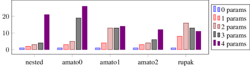
Figure 6: Fragmentation.

Figure 6 shows the number of regions in the results with different behavior. For the 0 parameter case this is always 1. As expected, the fragmentation increases with the number of parameters — but not as excessively as we expected. In case of rupak, the number of regions even decreased for three and four parameters. The reason is that by introducing fresh parameters, also the ordering on inequalities changes. The ordering on the other hand may have a significant impact onto fragmentation.

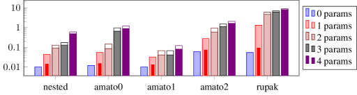
Figure 7: Execution time in (s).

Figure 7 shows the running times of the benchmarks on a logarithmic scale. We visualize the run-times for 0 through 4 parameters each. The filled and outlined bars correspond to Fourier-Motzkin elimination and integer satisfiability for testing emptiness of regions, respectively. The inscribed red bars in the single parameter case represent the run-time obtained by using linear lists instead of region trees. The bottom-line case without parameters is fast and the dedicated implementation for single parameters increases the run-time only by a factor of approximately 1.4. Using region trees clearly incurs an extra penalty, which increases significantly with the number of parameters. While replacing Fourier-Motzkin elimination for testing emptiness of regions with an enhanced algorithm for integer satisfiability increases the run-time only by an extra factor of about 1.5. When considering absolute run-times, however, it turns out that the solver even for four parameters together with full integer satisfiability is not prohibitively slow (a few seconds only for all benchmark equation systems). Details on experimental results can be found at www2.in.tum.de/~seidl/psi.

0.7 Related Work

Parametric analysis of linear numerical program properties has been advocated by Monniaux [22, 23] by compiling the abstract program semantics to real linear arithmetic and then use quantifier elimination to determine the parametric invariants. We have conducted experiments with Monniaux’ tool Mjollnir, by which we tried to solve real relaxations of parametric integer equations. Since Mjollnir has no native support for positive or negative infinities these values had to be encoded through formulas with extra propositional variables. This approach, however, did not scale to the sizes we needed. Our conjecture is that the high Boolean complexity of the formulas causes severe problems. Beyond that, fewer calls to quantifier elimination for formulas with many variables (as required by Mjollnir) may be more expensive than many calls to an integer solver for formulas with few variables (namely, the parameters as in our approach). All in all, since our integer tool and Mjollnir tackle slightly different problems, a precise comparison is difficult. Still, our experiments indicates that our approach behaves better than a quantifier elimination-based approach for applications where the control-flow is complex with multiple control-flow points, but where few parameters are of interest.

Since long, relational program analyses, e.g., by means of polyhedra have been around [4, 2] which also allow to infer linear relationships between parameters and program variables. The resulting invariants, however, are convex and thus do not allow to differentiate between different linear dependencies in different regions. In order to obtain invariants as precise as ours, one would have to combine polyhedral domains with some form of trace partitioning [20]. These kinds of analysis, though, must rely on widening and narrowing to enforce termination, whereas our algorithms avoid widening and narrowing completely and directly compute least solutions, i.e., the best possible parametric invariants.

Parametric analysis of a different kind has also been proposed by Reineke [25] in the context of worst-case execution time (WCET). They rely on parametric linear programming as implemented by the PIP tool [7] and infer the dependence of the WCET on architecture parameters such as the chache size by means of black box sampling of the WCETs obtained for different parameter settings.

Our data structure of region trees is a refinement of the tree-like data-structure Quast provided by the PIP tool [7]. Similar data-structures are also used by Monniaux [22] to represent the resulting invariants, and by Mihaila et al. [21] to differentiate between different phases of a loop iteration. In our implementation, we additionally enforce a total ordering on the constraints in the tree nodes and allow arbitrary values at the leaves. Total orderings on constraints have also been proposed for linear decision diagrams [3]. Variants of LDDs later have been used to implement non-convex linear program invariants [13, 12] and in [14] for representing linear arithmetic formulas when solving predicate abstraction queries. In our application, sharing of subtrees is not helpful, since each node $v$ represents a satisfiable conjunction of the inequalities which is constituted by the path reaching $v$ from the root of the data-structure. Moreover, our application requires that the leaves of the data-structure are not just annotated with a Boolean value (as for LDDs), but with values from various sets, namely strategic choices, affine functions or even pairs thereof.

0.8 Conclusion

Solving systems of parametric integer equations allows to solve also systems of parametric interval equations, and thus to realize parametric program analysis for programs using integer variables. To solve parametric integer equations, we have presented parametric strategy iteration. Instead of solving integer optimization and satisfiability problems involving all unknowns of the problem formulation (as an approach based on quantifier elimination), our algorithm is a smooth generalization of ordinary strategy iteration, which applies integer satisfiability to inequalities involving parameters only. Our prototypical implementation indicates that this approach indeed has the potential to deal with nontrivial problems — at least when only few parameters are involved. Introducing further parameters significantly increases the analysis costs. Surprisingly, the number of strategies required as well as the fragmentation observed in our examples increased only moderately. Accordingly, the required running times were quite decent.

More experiments are necessary, though, to obtain a deeper understanding of parametric strategy iteration. Also, we are interested in exploring the practical potential of sensitivity and mode analysis enabled by this new algorithm, e.g., for automotive and avionic applications.

Acknowledgement. We thank Stefan Barth (LMU) for Example 4, and Jan Reineke (Universität des Saarlandes) for useful discussions.

References

- [1] Gianluca Amato and Francesca Scozzari. Localizing widening and narrowing. In Static Analysis Symposium, volume 7935 of LNCS, pages 25–42. Springer, 2013.
- [2] Roberto Bagnara, Patricia M. Hill, and Enea Zaffanella. The Parma polyhedra library: Toward a complete set of numerical abstractions for the analysis and verification of hardware and software systems. Sci. Comput. Program., 72(1–2):3–21, 2008.
- [3] Sagar Chaki, Arie Gurfinkel, and Ofer Strichman. Decision diagrams for linear arithmetic. In Formal Methods in Computer-Aided Design, pages 53–60. IEEE Press, 2009.
- [4] Patrick Cousot and Nicolas Halbwachs. Automatic discovery of linear restraints among variables of a program. In Principles of Programming Languages, pages 84–96. ACM Press, 1978.
- [5] Isil Dillig, Thomas Dillig, and Alex Aiken. Cuts from proofs: A complete and practical technique for solving linear inequalities over integers. In Computer Aided Verification, volume 5643 of LNCS, pages 233–247. Springer, 2009.
- [6] Paul Feautrier. Parametric integer programming. RAIRO Recherche Opérationnelle, 22:243–268, 1988.
- [7] Paul Feautrier, Jean-François Collard, and Cédric Bastoul. A Solver for Parametric Integer Programming Problems, 2007.
- [8] Thomas Gal and Harvey J. Greenberg, editors. Advances in Sensitivity Analysis and Parametric Programming. Kluwer Academic Publishers, 1997.
- [9] Thomas Gawlitza and Helmut Seidl. Precise fixpoint computation through strategy iteration. In Programming Languages and Systems, volume 4421 of LNCS, pages 300–315. Springer, 2007.
- [10] Thomas Gawlitza and Helmut Seidl. Precise interval analysis vs. parity games. In Formal Methods, volume 5014 of LNCS, pages 342–357. Springer, 2008.
- [11] Thomas Gawlitza and Helmut Seidl. Abstract interpretation over zones without widening. In Workshop on Invariant Generation, volume 1 of EPiC, pages 12–43. EasyChair, 2012.
- [12] Khalil Ghorbal, Franjo Ivancic, Gogul Balakrishnan, Naoto Maeda, and Aarti Gupta. Donut domains: Efficient non-convex domains for abstract interpretation. In Verification, Model Checking, and Abstract Interpretation, volume 7148 of LNCS, pages 235–250. Springer, 2012.
- [13] Arie Gurfinkel and Sagar Chaki. Boxes: A symbolic abstract domain of boxes. In Static Analysis Symposium, volume 6337 of LNCS, pages 287–303. Springer, 2010.
- [14] Arie Gurfinkel, Sagar Chaki, and Samir Sapra. Efficient predicate abstraction of program summaries. In NASA Formal Methods, volume 6617 of LNCS, pages 131–145. Springer, 2011.
- [15] D. Halperin. Arrangements. In Joseph O’Rourke Jacob E. Goodman, editor, Handbook of Discrete and Computational Geometry (2nd Edition), chapter 24, pages 529–562. CRC Press, Inc., 2004.
- [16] A. Holder. Parametric LP analysis. Encyclopedia of Operations Research and Management Science, 2011.
- [17] Leonid G. Khachiyan. Polynomial algorithms in linear programming. USSR Computational Mathematics and Mathematical Physics, 20(1):53–72, 1980.
- [18] H.W. Lenstra, A.K. Lenstra, and L. Lovász. Factoring polynomials with rational coefficients. Mathematische Annalen, 261:515–534, 1982.
- [19] Jesús A. De Loera, David Haws, Raymond Hemmecke, Peter Huggins, and Ruriko Yoshida. Three kinds of integer programming algorithms based on Barvinok’s rational functions. In Integer Programming and Combinatorial Optimization, volume 3064 of LNCS, pages 244–255. Springer, 2004.
- [20] L. Mauborgne and X. Rival. Trace partitioning in abstract interpretation based static analyzers. In European Symposium on Programming, volume 3444 of LNCS, pages 5–20. Springer, 2005.
- [21] B. Mihaila, A. Sepp, and A. Simon. Widening as abstract domain. In NASA Formal Methods, volume 7871 of LNCS, pages 170–186. Springer, 2013.
- [22] David Monniaux. Automatic modular abstractions for linear constraints. In Principles of Programming Languages, pages 140–151. ACM Press, 2009.
- [23] David Monniaux. Quantifier elimination by lazy model enumeration. In Computer Aided Verification, volume 6174 of LNCS, pages 585–599. Springer, 2010.
- [24] William Pugh. The omega test: a fast and practical integer programming algorithm for dependence analysis. In Supercomputing, pages 4–13. IEEE Press, 1991.
- [25] Jan Reineke and Johannes Doerfert. Architecture-parametric timing analysis. In Real-Time and Embedded Technology and Applications Symposium, April 2014. To appear.