Effect of transitions in the Planck mass during inflation
on primordial power spectra

Abstract

We study the effect of sudden transitions in the effective Planck mass during inflation on primordial power spectra. Specifically, we consider models in which this variation results from the non-minimal coupling of a Brans-Dicke type scalar field. We find that the scalar power spectra develop features at the scales corresponding to those leaving the horizon during the transition. In addition, we observe that the tensor perturbations are largely unaffected, so long as the variation of the Planck mass is below the percent level. Otherwise, the tensor power spectra exhibit damped oscillations over the same scales. Due to significant features in the scalar power spectra, the tensor-to-scalar ratio $r$ shows variation over the corresponding scales. Thus, by studying the spectra of both scalar and tensor perturbations, one can constrain sudden but small variations of the Planck mass during inflation. We illustrate these effects with a number of benchmark single- and two-field models. In addition, we comment on their implications and the possibility to alleviate the tension between the observations of the tensor-to-scalar ratio performed by the Planck and BICEP2 experiments.

I Introduction

Aside from resolving a number of issues in the standard hot Big Bang scenario (see e.g. Sarkar:1995dd ; Lyth:1998xn ; LiddleLyth ; Baumann:2014nda ), including the horizon problem and overabundance of magnetic monopoles, inflationary cosmology has made a number of predictions consistent with current observations of the Cosmic Microwave Background (CMB). These include the expectation of an almost spatially-flat universe and an approximately scale-invariant power spectrum of the primordial curvature perturbations, as confirmed by the Wilkinson Microwave Anisotropy Probe (WMAP) Hinshaw:2012aka and, more recently, the Planck Satellite Ade:2013uln .

Many models of inflation also predict a cosmological gravitational wave background, parametrized in terms of the tensor-to-scalar ratio $r$. Recently, the BICEP2 experiment Ade:2014xna reported a detection of B-mode polarization in the CMB. When interpreted as being produced by such a background of primordial gravitational waves, this translates into a tensor-to-scalar ratio of

$$r=0.20^{+0.07}_{-0.05}\;,$$ (1)

around $\ell\simeq 80$, i.e. $k_{\rm BICEP}\simeq 0.005~{}{\rm Mpc}^{-1}$. This would be in tension with the previous limit set by Planck Ade:2013uln of $r\leq 0.11$ ($95\%$ C.L.) at the pivot scale $k_{0}\simeq 0.002~{}{\rm Mpc}^{-1}$, i.e. $\ell\simeq 28$. Such a value for the amplitude of the gravitational wave background would determine the scale of inflation to be at the GUT scale. Moreover, a value of $r\geq 0.1$ would rule out a large number of inflationary models in which the displacement of the field is smaller than $M_{\rm Pl}$ Lyth:1996im ; Hotchkiss:2011gz ; Antusch:2014cpa . Super-Planckian excursion of the inflaton field can be realized within a number of models, including assisted inflation Liddle:1998jc ; Kanti:1999vt ; Copeland:1999cs ; Mazumdar:2001mm ; Jokinen:2004bp , natural inflation Freese:1990rb ; Adams:1992bn ; Kim:2004rp , string-inspired many-field models Dimopoulos:2005ac ; Ashoorioon:2009wa ; Ashoorioon:2011ki ; Ashoorioon:2014jja and monodromy Silverstein:2008sg ; McAllister:2014mpa ; Hebecker:2014eua . In addition, values of $r>0.11$ can be realized in scalar models in which the potential has flat directions Ballesteros:2014yva .

Many authors have proposed solutions to alleviate the tension between BICEP2 and Planck on both theoretical Wang:2014kqa ; Ashoorioon:2014nta ; McDonald:2014kia ; Kawasaki:2014fwa ; Xu:2014laa ; Bastero-Gil:2014oga ; Cai:2014hja ; Mukohyama:2014gba and experimental grounds Liu:2014mpa ; Mortonson:2014bja ; Flauger:2014qra . In non-singular bouncing cosmologies Mukhanov:1991zn , it was shown Xia:2014tda that the emergence of jump features in the scalar and tensor power spectra at a given scale may conspire to lessen this discrepancy. This tension can also be alleviated in Starobinsky models Starobinsky:1992ts , if the speed of the inflaton field undergoes a sudden change Contaldi:2014zua . In addition, sharp features are observed in the scalar power spectra in models of punctuated inflation, where the shape of the inflaton potential changes discontinuously at a given scale Jain:2008dw ; Jain:2009pm ; Hazra:2010ve . An inflaton potential with a step was studied in the Einstein frame Adams:2001vc (see also Joy:2007na ) and shown to result in oscillations in the power spectra. Fading oscillatory features in the primordial scalar power spectrum can also occur from jumps in the potential Ashoorioon:2006wc ; Ashoorioon:2008qr ; Firouzjahi:2014fda ; Bartolo:2013exa ; Battefeld:2010rf , particle production during inflation Barnaby:2010ke ; Battefeld:2010vr ; Battefeld:2013bfl or turns in the inflaton trajectory in the landscape of heavy fields Cespedes:2012hu ; Achucarro:2012fd ; Cespedes:2013rda ; Saito:2013aqa ; Konieczka:2014zja . For a discussion of observed features in the primordial power spectrum, see for instance Aslanyan:2014mqa and references therein.

Recently, there has also been renewed interest in models of inflation with time-varying gravitational constants Abolhasani:2012tz . The potential time-dependence of physical constants has long been recognized Dirac:1937ti and variation in the effective gravitational coupling is known to arise in theories of modified gravity, such as Brans-Dicke Scalar-Tensor Brans:1961sx ; Fujii:1974bq ; Minkowski:1977aj ; Linde:1979kf ; Fujii:1982ms ; DeFelice:2011hq and Tensor-Vector-Scalar (TeVeS) theory Bekenstein:2004ne ; Bekenstein:2008pc . The latter provides a relativistic basis for Milgrom’s Modified Newtonian Dynamics (MOND) Milgrom:1983ca . Time-dependency may also arise in Supersymmetric String Theories Wu:1986ac ; Ivashchuk:1988bs ; Ivashchuk:2014rga .

The implications of a time-varying gravitational constant (see also Uzan:2010pm ) have been studied in the radiation and matter dominated epochs Wetterich:1987fk . It was shown in Accetta:1990yb that modulations of the gravitational constant can result from the non-minimal coupling of a massive scalar field that oscillates around its vacuum expectation value (VEV). It was found that cosmological measurements can be affected when the frequency of oscillations is high compared to the Hubble expansion rate. This work was extended in Steinhardt:1994vs to consider a scenario in which the Brans-Dicke field is driven away from its VEV during inflation, thereby inducing oscillations. For cosmological perturbation theory in models beyond General Relativity, see Mukhanov:1990me , Hwang:2005hb and references therein.

There are various experiments that test models with a time-dependent Newton’s constant: lunar ranging observations Williams:2004qba ; Muller:2007zzb , Big Bang Nucleosynthesis (BBN) Copi:2003xd ; Santiago:1997mu ; Bambi:2005fi ; Coc:2006rt , gravitational waves Yunes:2009bv and, more recently, the WiggleZ experiment Nesseris:2011pc . In addition, it has been shown that the late-time evolution of the gravitational constant can be constrained through comparisons of the ages of globular clusters with independent measurements of the age of the Universe Degl'Innocenti:1995nt and by observations of type 1a supernovae GarciaBerro:2005yw ; Nesseris:2006jc , as well as pulsating white dwarfs GarciaBerro:2011wc ; Corsico:2013ida , pulsars BisnovatyiKogan:2005ap ; Jofre:2006ug ; Verbiest:2008gy ; Lazaridis:2009kq and neutron-star surface temperatures Krastev:2007en . Such limits on the variation of the gravitational constant place constraints on scalar-tensor theories Babichev:2011iz in addition to those obtained from observations of primordial density perturbations Chiba:1997ij ; Tsujikawa:2000wc ; Lee:2010zy and gravitational Cherenkov radiation Kimura:2011qn .

In this article, we show that sharp features may arise in the scalar power spectra as a result of transitions in the effective Planck mass (or equivalently Newton’s gravitational constant) during inflation. Specifically, we address the question of whether smooth step variations in the gravitational coupling, occurring during the observable window of scales between 60 and 50 $e$-folds before the end of inflation Turner:1993xz ; Liddle:2003as , have sizeable effects on the power spectra for curvature and tensor perturbations. Step changes in the Planck mass could result from a first-order phase transition in the VEV of a Brans-Dicke field Abolhasani:2012tz . Alternatively, as we will consider, the step change could arise through a second-order transition, with the Brans-Dicke field rolling slowly towards its VEV. We consider two scenarios: one in which the role of Brans-Dicke field is played by the inflaton itself and a two-field model in which this role is played by a second auxiliary field. The variations that we have in mind are not violent ones, i.e. the variations of $M_{\rm Pl}$ are not of order $1$. Instead, they are typically of order a percent or less. Nevertheless, we illustrate that, for a particular choice of parameters for the single-field model, the impact upon the resulting power spectra and, consequently, the tensor-to-scalar ratio $r$ has the potential to alleviate the aforementioned discrepancy between BICEP2 and Planck. Furthermore, in contrast to potentials with a step Adams:2001vc , we show that oscillations are not observed in the scalar power spectra when the step transition occurs instead in the non-minimal coupling of the Brans-Dicke field.

The paper is organized as follows. In Sec. II, we describe the relevant background field and perturbation equations for the single-field model under consideration. In Sec. III, we solve these systems of equations numerically for a number of single- and two-field benchmark models, illustrating the potential implications for observations of primordial power spectra. Finally, in Sec. IV, we provide our conclusions. In addition, App. A summarizes the background and perturbation equations for the two-field model considered and App. B describes the approximate analytic solutions to the background evolution, relevant to Sec. III.

II Field equations

Our goal is to study the influence of variations in the effective Planck mass (or equivalently Newton’s gravitational constant) on inflation and the primordial power spectra for scalar and tensor perturbations. This can be described conveniently in the context of scalar-tensor theories. Specifically, we will focus on the case in which the evolution of the inflaton itself causes this variation by means of its non-minimal coupling to the Ricci scalar. For this reason and throughout this article, we choose to perform the computations in the Jordan frame, which allows us to model these variations in the Planck mass intuitively. Nevertheless, physical observables do not depend on the choice of frame (see e.g. Kaiser:1994vs ; Kaiser:1995nv ; Prokopec:2013zya and references therein) and hence equivalent results would be obtained in the Einstein frame.

The single-field action that we consider is of the form

$$S^{(\varphi)}\ =\ \frac{1}{2}\int d^{4}x\sqrt{-g}\bigg{[}M_{\rm Pl}^{2}F(\varphi)R-g^{\mu\nu}\varphi_{,\mu}\varphi_{,\nu}-2U(\varphi)\bigg{]}\;,$$ (2)

where $M_{\rm Pl}^{2}=(8\pi G_{\ast})^{-1}$ is the reduced Planck mass, with $G_{*}$ being the present-day Newton’s constant; $R$ is the Ricci scalar and $U(\varphi)$ is the potential of the scalar field $\varphi$. Hereafter, we set $M_{\rm Pl}=1$, with all dimensionful quantities understood to be in units of the reduced Planck mass. The coupling of gravity to other energy and matter degrees of freedom is then determined by the effective Planck mass $F(\varphi)$.

Varying the action Eq. (2) with respect to the metric, we obtain the Einstein equations, which are given by

$$G_{\mu\nu}=\frac{1}{F(\varphi)}\bigg{[}\varphi_{,\mu}\varphi_{,\nu}-\frac{1}{2}g_{\mu\nu}g^{\alpha\beta}\varphi_{,\alpha}\varphi_{,\beta}+F_{;\mu\nu}(\varphi)-g_{\mu\nu}\Box F(\varphi)-g_{\mu\nu}U(\varphi)\bigg{]}\;,$$ (3)

where $G_{\mu\nu}$ is the Einstein tensor, $\Box$ is the d’Alembertian operator and $,\mu$ and $;\mu$ denote partial and covariant derivatives with respect to the spacetime coordinate $x^{\mu}$, respectively. Varying the action with respect to the scalar field $\varphi$ yields the Klein-Gordon equation, written in Brans-Dicke form as

$$2\varpi(\varphi)\Box\varphi(\varphi)=-\varpi_{,\varphi}(\varphi)g^{\mu\nu}\varphi_{,\mu}\varphi_{,\nu}-4F_{,\varphi}(\varphi)U(\varphi)+2F(\varphi)U_{,\varphi}(\varphi)\;,$$ (4)

where we have defined $\varpi(\varphi)=F(\varphi)+\frac{3}{2}F_{,\varphi}^{2}(\varphi)$, in which $,\varphi$ denotes partial differentiation with respect to the scalar field $\varphi$. Hereafter, we will omit arguments on the functions of the scalar field for notational convenience.

II.1 Background

We shall assume a spatially homogeneous and isotropic background spacetime, described by the Friedmann-Robertson-Walker (FRW) line element

$$\mathrm{d}s^{2}=-\mathrm{d}t^{2}+a^{2}(t)\delta_{ij}\mathrm{d}x^{i}\mathrm{d}x^{j}\;,$$ (5)

where $\delta_{ij}$ is the Kronecker delta and $a(t)$ is the scale factor. In FRW space-time, Eq. (4) is then

$$\ddot{\varphi}+3H\dot{\varphi}=\frac{1}{2\varpi}[-\varpi,_{\varphi}\dot{\varphi}^{2}+4F,_{\varphi}U-2FU,_{\varphi}]\;,$$ (6)

where $\dot{}$ denotes differentiation with respect to the cosmic time $t$ and $H=\dot{a}/a$ is the Hubble parameter. Furthermore, the Friedmann equations take the form

$$H^{2} =\frac{1}{3F}\bigg{[}\frac{1}{2}\dot{\varphi}^{2}+U-3H\dot{F}\bigg{]}\;,$$ (7a)

$$-2\dot{H} =\frac{1}{F}\bigg{[}\dot{\varphi}^{2}+\ddot{F}-H\dot{F}\bigg{]}\;.$$ (7b)

Equations (3), (6) and (7) suggest to define an effective energy density $\rho$ and pressure $p$ for the scalar field as follows:

$$\rho =\frac{1}{F}\bigg{[}\frac{1}{2}\dot{\varphi}^{2}+U-3H\dot{F}\bigg{]}\;,$$ (8a)

$$p =\frac{1}{F}\bigg{[}\frac{1}{2}\dot{\varphi}^{2}-U+\ddot{F}+2H\dot{F}\bigg{]}\;.$$ (8b)

We note that these are effective quantities and that the corresponding energy-momentum tensor $T^{(\varphi)}_{\mu\nu}$ is conserved, i.e. $T_{\mu\nu}^{(\varphi);\mu}=0$.

In order to test the generalities of the single–field results, we consider a two-field model, in which the action Eq. (2) is supplemented with an additional minimally-coupled scalar $\chi$ with action

$$S^{(\chi)}\ =\ -\>\frac{1}{2}\int d^{4}x\sqrt{-g}\bigg{[}g^{\mu\nu}\chi_{,\mu}\chi_{,\nu}+2V(\chi)\bigg{]},$$ (9)

where the potential $V(\chi)$ is given by

$$V(\chi)\ =\ \frac{1}{2}m_{\chi}^{2}\chi^{2}\;.$$ (10)

The pertinent background field and perturbation equations for the two-field model $S=S^{(\varphi)}+S^{(\chi)}$ are summarized in App. A.

II.2 Perturbations

II.2.1 Scalar perturbations

We will now focus our attention on the first-order perturbation equations, which will be studied in the Newtonian gauge. In this gauge, the scalar metric perturbations are expressed by the following line element, cf. Eq. (5),

$$ds^{2}=-(1+2\Psi)\mathrm{d}t^{2}+a(t)^{2}(1-2\Phi)\delta_{ij}\mathrm{d}x^{i}\mathrm{d}x^{j}\;,$$ (11)

where $\Psi$ and $\Phi$ are the scalar metric perturbations.

The scalar field $\varphi(t,\mathbf{x})$ is decomposed in terms of the homogeneous background contribution $\varphi(t)$ and the perturbation $\delta\varphi(t,\mathbf{x})$, i.e.

$$\varphi(t,\mathbf{x})=\varphi(t)+\delta\varphi(t,\mathbf{x})\;.$$ (12)

Thereafter, we work with the Fourier components of the perturbations, $\delta\varphi_{k}(t)$, satisfying $\nabla^{2}\delta\varphi_{k}=-k^{2}\delta\varphi_{k}$. In what follows, the subscript $k$ will be omitted in order to shorten the subsequent expressions.

The resulting perturbation equation for the scalar field is

$$\delta\ddot{\varphi} +\bigg{[}3H+\frac{\varpi,_{\varphi}}{\varpi}\dot{\varphi}\bigg{]}\delta\dot{\varphi}+\bigg{[}\frac{1}{2}\bigg{(}\frac{\varpi,_{\varphi}}{\varpi}\bigg{)}_{\!\!,\varphi}\!\dot{\varphi}^{2}-\frac{1}{2}\bigg{(}\frac{1}{\varpi}(4F,_{\varphi}U-2FU,_{\varphi})\bigg{)}_{\!\!,\varphi}+\frac{k^{2}}{a^{2}}\bigg{]}\delta\varphi$$

$$-(\dot{\Psi}+3\dot{\Phi})\dot{\varphi}+\frac{1}{\varpi}\bigg{[}-4F_{,\varphi}U+2FU_{,\varphi}\bigg{]}\Psi=0\;.$$ (13)

Additionally, in the Newtonian gauge, the perturbed Einstein equations are given by the following:

$$3H(\dot{\Phi}+H\Psi)+\frac{k^{2}}{a^{2}}\Phi =-\frac{1}{2}\delta\rho\;,$$ (14a)

$$\dot{\Phi}+H\Psi =-\frac{1}{2}\delta q\;,$$ (14b)

$$\ddot{\Phi}+(2\dot{H}+3H^{2})\Psi+H(\dot{\Psi}+3\dot{\Phi}) =\frac{1}{2}\delta p\;,$$ (14c)

where $\delta\rho$, $\delta q$ and $\delta p$, obtained from the effective energy-momentum tensor $T_{\mu\nu}$ mentioned earlier, are the perturbations in the energy density, momentum potential and pressure, respectively:

$$\delta\rho =\frac{1}{F}\bigg{[}\dot{\varphi}\delta\dot{\varphi}-\dot{\varphi}^{2}\Psi+U,_{\varphi}\delta\varphi+\,3\dot{F}(\dot{\Phi}+2H\Psi)-3H(\delta\dot{F}+H\delta F)-\frac{k^{2}}{a^{2}}\delta F\bigg{]}\;,$$ (15a)

$$\delta q =-\frac{1}{F}\bigg{[}\dot{\varphi}\delta\varphi+\delta\dot{F}-\dot{F}\Psi-H\delta F\bigg{]}\;,$$ (15b)

$$\delta p =\frac{1}{F}\bigg{[}\dot{\varphi}\delta\dot{\varphi}-\dot{\varphi}^{2}\Psi-U,_{\varphi}\delta\varphi-\,p\,\delta F+\delta\ddot{F}+2H\delta\dot{F}-\dot{F}\dot{\Psi}-2\dot{F}\dot{\Phi}$$

$$\qquad-\,2(\ddot{F}+2H\dot{F})\Psi+\frac{k^{2}}{a^{2}}\delta F\bigg{]}\;.$$ (15c)

Hence, we find that anisotropic stress is present in the Jordan frame with

$$\Phi-\Psi=\frac{\delta F}{F}=\frac{F_{,\varphi}\delta\varphi}{F}\;.$$ (16)

The observational quantities include the spectral index $n_{s}$ and its running $\alpha$, which can be obtained from the curvature (scalar) power spectra by using Kosowsky:1995aa ; Hinshaw:2012aka

$$\mathcal{P}_{\zeta}(k)=\mathcal{P}_{\zeta}(k_{0})\bigg{(}\frac{k}{k_{0}}\bigg{)}^{n_{s}(k_{0})-\,1+\frac{1}{2}\ln(k/k_{0})\,\alpha}\;.$$ (17)

The scalar perturbations

$$\mathcal{P}_{\zeta}\ =\ \frac{k^{3}}{2\pi^{2}}|\zeta|^{2}$$ (18)

are provided by the curvature perturbation on constant hypersurfaces $\zeta$, defined via

$$\zeta=-\,\Phi-\frac{H}{\dot{\rho}}\delta\rho\;.$$ (19)

At the Planck pivot scale $k_{0}$, the amplitude of the power spectrum is $\mathcal{P}_{\zeta}(k_{0})\sim 2.15\times 10^{-9}$ Ade:2013uln . The running index $\alpha$, in relation to the spectral index $n_{s}$, is given by

$$\alpha=\frac{d\,n_{s}}{d\,\mathrm{ln}k}\;.$$ (20)

The current best fit values for both the spectral index and its running, as measured by Planck Ade:2013uln , are

$$n_{s}=0.9603\pm 0.0073~{},\qquad\qquad\alpha=-\,0.0134\pm 0.0090\;.$$ (21)

II.2.2 Tensor perturbations

We shall also study the effect of variations in the Planck mass on tensor perturbations. The equations for the tensor modes take the standard form, since they are not affected by the presence of the non-minimal coupling $F(\varphi)$. Specifically, the power spectrum for the tensor perturbations is given by Habib:2005mh

$$\mathcal{P}_{\mathrm{T}}\ =\ \frac{k^{3}}{2\pi^{2}}\bigg{|}\frac{v_{k}}{a}\bigg{|}^{2}~{},$$ (22)

where the mode equation for gravitational waves takes the form

$$v_{k}^{\prime\prime}+\bigg{(}k^{2}-\frac{a^{\prime\prime}}{a}\bigg{)}v_{k}\ =\ 0\;,$$ (23)

in which the prime (^′) denotes the derivative with respect to conformal time $\eta=\int_{0}^{t}\frac{\mathrm{d}t^{\prime}}{a(t^{\prime})}$.

Finally, the tensor-to-scalar ratio $r$ is given in terms of the scalar and tensor power spectra $\mathcal{P}_{\mathrm{T}}$ and $\mathcal{P}_{\zeta}$, see Eqs. (18) and (22) via PeterUzan

$$r=\frac{8\mathcal{P}_{\mathrm{T}}}{\mathcal{P}_{\zeta}}~{}.$$ (24)

III Model with step variation in the Planck mass

In this section, we will consider models in which the effective Planck mass undergoes a step transition during the inflationary epoch. To this end, we consider the following non-minimal coupling and potential for a canonical Brans-Dicke scalar field:

$$F(\varphi) =1-\beta\,\{\,1+\tanh[(\varphi-\varphi_{\ast})/\gamma\,]\,\}\;,$$ (25)

$$U(\varphi) =\frac{1}{2}m_{\varphi}^{2}\varphi^{2}\;,$$ (26)

where $m_{\varphi}$ is the mass of the scalar field $\varphi$, $\beta$ is a dimensionless constant, and $\gamma$ and $\varphi_{\ast}$ are constants of mass dimension. As we shall see, the parameters $\beta$ and $\gamma$ determine the amplitude and sharpness of the transition in $F$ and $\varphi_{\ast}$ determines the field value at which the transition occurs. We have chosen the quadratic potential for concreteness. However, we should emphasize that the features observed in the forthcoming sections are anticipated to persist for other choices of the potential $U(\varphi)$.

In the first instance, we will consider a single field model, in which the Brans-Dicke field also drives inflation. Subsequently, we will consider a two-field model, in which a second minimally-coupled scalar field acts as the inflaton. Nevertheless, in both cases and for each of the benchmark models considered, the values of the parameters are chosen so as to obtain successful inflation, with the inflationary period lasting a total of 66 $e$-folds.

Before proceeding, we will now illustrate that the Jordan-frame model described above is not equivalent to an Einstein-frame model of an inflaton potential with a step, see Adams:2001vc . By means of a conformal transformation, we could transform the model in Eqs. (25) and (26) to the Einstein frame. Therein, the new potential for the Brans-Dicke field $\varphi$ would become

$$\tilde{U}(\varphi)\ =\ \frac{U(\varphi)}{F^{2}(\varphi)}\ =\ \frac{m_{\varphi}^{2}\varphi^{2}}{2\big{\{}1-\beta\,\{\,1+\tanh[(\varphi-\varphi_{\ast})/\gamma\,]\}^{2}}\;,$$ (27)

which resembles the step potential in Adams:2001vc for $\beta\ll 1$. Note however that we should anticipate different dynamics, since in the Einstein frame the kinetic term of the model we consider will not be of canonical form, as it is in Adams:2001vc . The canonical field $\tilde{\varphi}$ is related to the non-canonical $\varphi$ through the relation

$$\tilde{\varphi}=\int\sqrt{\frac{2F(\varphi)+3{F_{,\varphi}(\varphi)}^{2}}{2F(\varphi)^{2}}}~{}d\varphi.$$ (28)

Inverting the above equation, one can derive $\varphi$ in terms of $\tilde{\varphi}$, at least implicitly. Upon replacement of $\varphi$ in terms of $\tilde{\varphi}$ in $\tilde{U}(\varphi)$, the potential for the canonical field $\tilde{\varphi}$ could be obtained. However, the final form of the potential, written in terms of the canonical field $\tilde{\varphi}$, will not be the potential with a step Eq. (27). As such, we conclude that a step potential of a canonical field is not an appropriate phenomenological model of a Jordan-frame action in which the effective Planck mass undergoes a step change. Thus, the model under investigation here differs from those considered previously in the literature, leading to significantly different predictions for the scalar and tensor spectra.

Returning to the Jordan frame, the dynamics of the fields will be solved numerically, following the method outlined in Tsujikawa:2002qx ; the derivatives of the background fields are given their slow-roll values and the initial field perturbations will have the standard oscillatory Bunch-Davies initial conditions Adams:2001vc . In order to calculate the tensor perturbations generated by the system, we employ the methods described in Adams:2001vc ; Habib:2005mh .

In App. B, we use an approximate analytic solution to the background field equations in order to illustrate the dependence on the parameters $\beta$ and $\gamma$ of the resulting features in the slow-roll parameter $\varepsilon$. The latter allows us to infer the dependency on the same parameters of the features in the scalar power spectra $\mathcal{P}_{\zeta}$ and the tensor-to-scalar ratio $r$.

III.1 Single-field model

III.1.1 Minimally-coupled limit

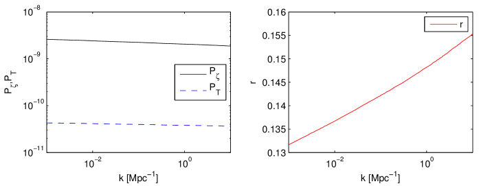
Figure 1: Power spectra (left) of scalar ($\mathcal{P}_{\zeta}$, solid black) and tensor perturbations ($\mathcal{P}_{\mathrm{T}}$, blue dashed) and the associated tensor-to-scalar ratio $r$ (right) against wavenumber $k$ (${\rm Mpc^{-1}}$) for the minimally-coupled scenario. The model parameters are $m_{\varphi}=6.5\times 10^{-6}$, with $\varphi_{\mathrm{ini}}=16.179$.

We first consider the minimally-coupled case, in which $\beta=0$, i.e. $F=1$. The value of the scalar field $\varphi$ at the start of inflation is taken to be $\varphi_{\mathrm{ini}}=16.179$. The mass of the scalar field is chosen to be $m_{\varphi}=6.5\times 10^{-6}$, so that the power spectrum for the scalar perturbations at the Planck pivot scale is approximately $2.15\times 10^{-9}$. The power spectra for the scalar and tensor perturbations are given in Fig. 1. Notice that we have defined the number of $e$-folds $N$ such that $N=0$ at the start of inflation.

There are no features generated in this model, as we would expect for minimally-coupled single-field inflation. The spectral and running indices are calculated to be

$$n_{s}=0.968865\;,\qquad\alpha=0.00107427\;.$$ (29)

In addition to this, the tensor-to-scalar ratio at the pivot scale $k_{0}$ is

$$r(k_{0})=0.133205$$ (30)

We have chosen a quadratic potential for simplicity. The model is under slight pressure from the Planck experiment Ade:2013uln (cf. Ashoorioon:2013eia , which attempts to reconcile this model with the Planck data), although it is still within the $68\%$ C.L. in the $n_{s}-r$ plane. Nevertheless, the phenomenological conclusions presented later in this paper do not depend heavily on the choice of potential.

III.1.2 Benchmark 1

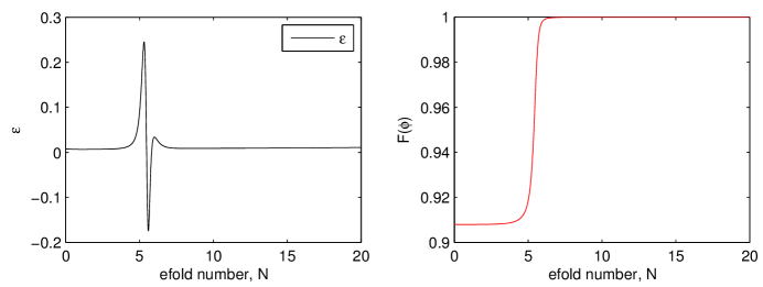
Figure 2: Evolution of the slow-roll parameter $\varepsilon$ (left) and the effective Planck mass $F$ (right) for the first $20$ $e$-folds of inflation in benchmark model 1. The model parameters are $m_{\varphi}=2.1\times 10^{-5}$, $\beta=0.0460$, $\gamma=0.145$ and $\varphi_{\ast}=15.8$, with $\varphi_{\mathrm{ini}}=16.5783$.

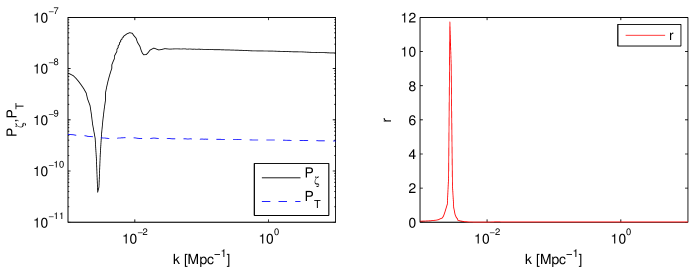
Figure 3: Power spectra (left) of scalar ($\mathcal{P}_{\zeta}$, solid black) and tensor perturbations ($\mathcal{P}_{\mathrm{T}}$, blue dashed) and the associated tensor-to-scalar ratio $r$ (right) against wavenumber $k$ (${\rm Mpc^{-1}}$) for benchmark model 1. The model parameters are $m_{\varphi}=2.1\times 10^{-5}$, $\beta=0.0460$, $\gamma=0.145$ and $\varphi_{\ast}=15.8$, with $\varphi_{\mathrm{ini}}=16.5783$.

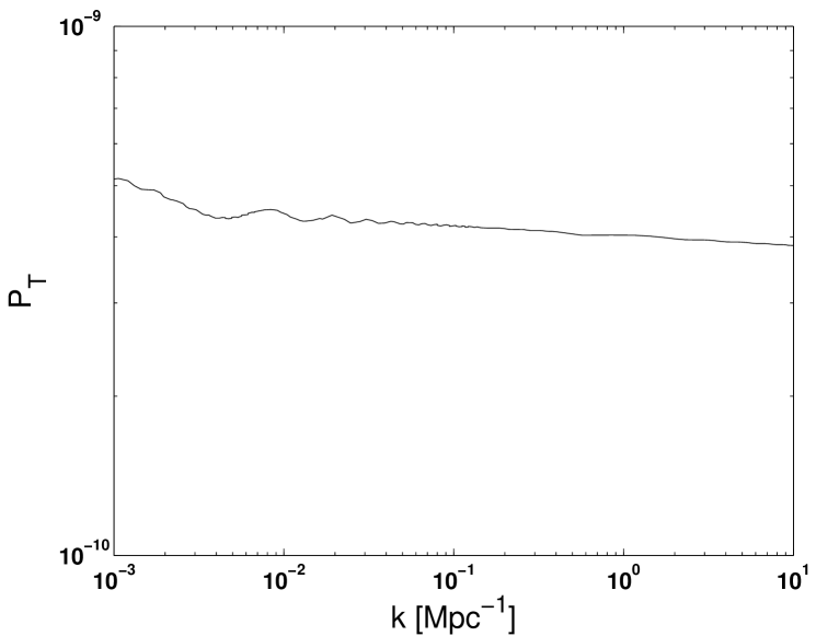
Figure 4: The power spectrum of tensor perturbations ($\mathcal{P}_{\mathrm{T}}$) showing the damped oscillations present for benchmark model 1. The model parameters are $m_{\varphi}=2.1\times 10^{-5}$, $\beta=0.0460$, $\gamma=0.145$ and $\varphi_{\ast}=15.8$, with $\varphi_{\mathrm{ini}}=16.5783$.

In this first benchmark model, we will consider a steep transition in the Planck mass, causing a violent feature in the slow-roll parameter $\varepsilon$. Specifically, the model parameters are $m_{\varphi}=2.1\times 10^{-5}$, $\beta=0.0460$, $\gamma=0.145$ and $\varphi_{\ast}=15.8$, with the initial field value $\varphi_{\mathrm{ini}}=16.5783$. The $e$-fold evolutions of $F$ and $\varepsilon$ are displayed in Fig. 2, in which we see a transient violation of slow-roll.

The resulting scalar and tensor power spectra are displayed in the left panel of Fig. 3. We see an extremely sharp dip in the power spectrum of the scalar perturbation at $k\sim 0.003~{}\mathrm{Mpc}^{-1}$. This feature and the smaller oscillation-like fluctuations that follow coincide with those observed in the slow-roll parameter in Fig. 2. Notice however that these features do not resemble the dramatic oscillations seen in inflationary models with a step potential, see Adams:2001vc . For this set of parameters, we also observe damped oscillations in the tensor power spectrum, as demonstrated in Fig. 4. However, the amplitude of this effect is significantly smaller than that of the feature in the scalar power spectrum.

These observations may be understood in terms of the behaviour of the slow-roll parameter $\varepsilon$. Specifically, in the single-field model, the scalar power spectrum $\mathcal{P}_{\zeta}\sim H^{2}/\varepsilon$, whereas $\mathcal{P}_{T}\sim H^{2}$. Hence, we see that the sharp rise in the slow-roll parameter leads to a sharp dip in the scalar power spectrum at the same scale, whilst leaving the tensor power spectrum largely unaffected.

The tensor-to-scalar ratio as a function of the wavenumber is presented in the right-hand side panel of Fig. 3. We see a sharp rise in $r$ at scales corresponding to the feature in the slow-roll parameter $\varepsilon$, since $r\sim\mathcal{P}_{T}/\mathcal{P}_{\zeta}\sim\varepsilon$. Although an unrealistically-large tensor-to-scalar ratio is generated in the region of the Planck pivot scale in this benchmark model, this can be useful in constraining the parameters of the non-minimal coupling $F$.

III.1.3 Benchmark 2

In this example, we show that one can produce features in the scalar power spectrum that reduce the tension between the tensor-to-scalar ratio $r$ observed by the Planck Ade:2013uln and BICEP2 Ade:2014xna experiments, as described in Sec. I. To this end, we choose the following set of model parameters: $m_{\varphi}=6.9\times 10^{-6}$, $\beta=0.002$, $\gamma=0.111$ and $\varphi_{\ast}=15.49$, with the initial field value $\varphi_{\mathrm{ini}}=16.2271$.

In Fig. 5, we see that the slow-roll parameter creates a peak due to the increase in the coupling at approximately $N=6$. Notice that, with this combination of parameters, the initial value of $F(\varphi_{\mathrm{ini}})=0.996$ deviates by less than $0.5\%$ from minimal coupling, compared with $\sim 10\%$ deviation in benchmark 1.

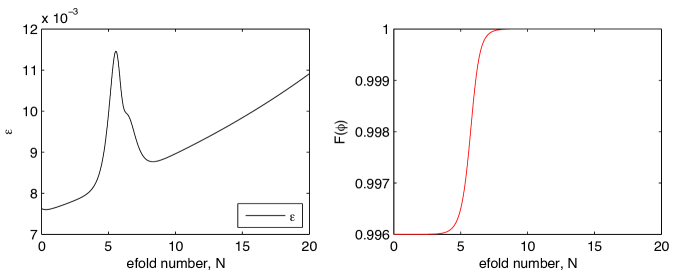
Figure 5: Evolution of the slow-roll parameter $\varepsilon$ (left) and the effective Planck mass $F$ (right) for the first $20$ $e$-folds of inflation in benchmark model 2. The model parameters are $m_{\varphi}=6.9\times 10^{-6}$, $\beta=0.002$, $\gamma=0.111$ and $\varphi_{\ast}=15.49$, with $\varphi_{\mathrm{ini}}=16.2271$.

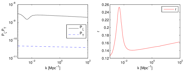
Figure 6: Power spectra (left) of scalar ($\mathcal{P}_{\zeta}$, solid black) and tensor perturbations ($\mathcal{P}_{\mathrm{T}}$, blue dashed) and the associated tensor-to-scalar ratio $r$ (right) against wavenumber $k$ (${\rm Mpc^{-1}}$) for benchmark model 2. The model parameters are $m_{\varphi}=6.9\times 10^{-6}$, $\beta=0.002$, $\gamma=0.111$ and $\varphi_{\ast}=15.49$, with $\varphi_{\mathrm{ini}}=16.2271$.

The resulting power spectra for the scalar and tensor perturbations are displayed in the left panel of Fig. 6 and the tensor-to-scalar ratio versus wavenumber in the right panel. As expected, a reduction in the power is observed. The tensor power spectrum, on the other hand, is unaffected. We see that, with this choice of parameters, the value of $r$ at $k\simeq 0.005~{}{\rm Mpc}^{-1}$, see Eq. (1), is consistent with the BICEP2 result, whilst maintaining agreement with the Planck limit of $r\leq 0.11$ at $k\simeq 0.002~{}{\rm Mpc}^{-1}$.

For $k>10^{-2}$, the value of the spectral tilt is $n_{s}\approx 0.98$. The maximum value of the spectral index in the vicinity of the feature is obtained by means of Stewart:1993bc

$$n_{s}(k)\ \approx\ 1+k\,\frac{\mathrm{d}}{\mathrm{d}k}\ln\,\mathcal{P}_{\zeta}(k)\;.$$ (31)

One can obtain a rough estimate on the maximum magnitude for the non-linearity parameter $f_{\mathrm{{NL}}}$ in the squeezed limit Maldacena:2002vr of

$$|f_{\mathrm{NL}}|_{\mathrm{max}}\ \approx\ \frac{5}{12}|1-n_{s}|\ \approx\ 0.45\;.$$ (32)

Thus, even in the vicinity of the transition, this model remains consistent with the Planck limit for local non-Gaussianity of $f_{\mathrm{NL}}^{\mathrm{loc}}\>=\>2.7\pm 5.8$ Ade:2013ydc .

III.1.4 Benchmark 3

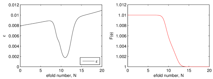
Figure 7: Evolution of the slow-roll parameter $\varepsilon$ (left) and the effective Planck mass $F$ (right) for the first $20$ $e$-folds of inflation in benchmark model 3. The model parameters are $m_{\varphi}=6.5\times 10^{-6}$, $\beta=-0.005$, $\gamma=0.100$ and $\varphi_{\ast}=14.64$, with $\varphi_{\mathrm{ini}}=15.9055$.

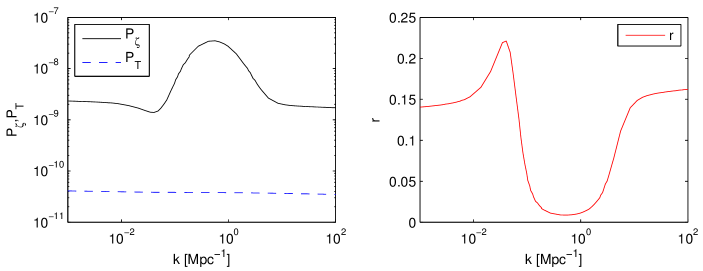
Figure 8: Power spectra (left) of scalar ($\mathcal{P}_{\zeta}$, solid black) and tensor perturbations ($\mathcal{P}_{\mathrm{T}}$, blue dashed) and the associated tensor-to-scalar ratio $r$ (right) against wavenumber $k$ (${\rm Mpc^{-1}}$) for benchmark model 3. The model parameters are $m_{\varphi}=6.5\times 10^{-6}$, $\beta=-0.005$, $\gamma=0.100$ and $\varphi_{\ast}=14.64$, with $\varphi_{\mathrm{ini}}=15.9055$.

Finally, to illustrate the enhancement of power over certain scales, we consider the case in which the the factor $\beta$ is negative. The model parameters chosen are $m_{\varphi}=6.5\times 10^{-6}$, $\beta=-0.005$, $\gamma=0.100$ and $\varphi_{\ast}=14.64$, with the initial field value $\varphi_{\mathrm{ini}}=15.9055$.

The evolutions of the slow-roll parameter $\varepsilon$ and coupling $F(\varphi)$ for this choice of parameters are displayed in Fig. 7. We see that the change in sign of $\beta$ causes a dip in the evolution of the slow-roll parameter, which lasts approximately $7$ $e$-folds for this set of parameters. As we would anticipate given the earlier examples, this results in a region of enhancement in the scalar power spectrum. The scalar power spectrum is shown in the left panel of Fig. 8. In addition, Fig. 8 presents both the scalar and tensor power spectra as well as the gravitational coupling as functions of wavenumber. There is no considerable effect upon the tensor power spectrum. From the right panel of Fig. 8, we see that the enhancement in the scalar power spectrum suppresses the tensor-to-scalar ratio in the range: $10^{-1}~{}{\rm Mpc^{-1}}<k<10^{1}~{}{\rm Mpc^{-1}}$ compared with the enhancement for $10^{-2}~{}{\rm Mpc^{-1}}<k<10^{-1}~{}{\rm Mpc^{-1}}$, corresponding to the initial suppression of power.

III.2 Two-field model

In this section, we calculate the power spectra of a two-field model directly in the Jordan frame. The transition in the Planck mass results again from the Brans-Dicke scalar $\varphi$, see Eq. (2), whilst inflation is instead driven dominantly by an additional minimally-coupled scalar $\chi$, see Eq. (9).

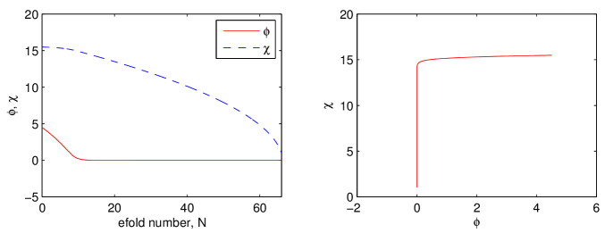
Figure 9: Evolution of $\varphi$ and $\chi$ versus $e$-fold number $N$ (left) and the field trajectory in the $\varphi$-$\chi$ plane for the same $e$-foldings, illustrating the sharp turn at $N\sim 10$ (right).

The model parameters chosen are $m_{\chi}=5.6\times 10^{-6}$, $m_{\varphi}=4.48\times 10^{-5}$, $\beta=0.009$, $\gamma=0.111$ and $\varphi_{\ast}=1.0$. The initial field values are $\varphi_{\mathrm{ini}}=4.5$ and $\chi_{\mathrm{ini}}=15.489$. Figure 9 shows the evolution of the Brans-Dicke field $\varphi$ and the scalar $\chi$. Therein and for these model parameters, it is clear that the last $50$ $e$-folds of inflation are driven by the would-be inflaton field $\chi$. The evolutions of the slow-roll parameter $\varepsilon$ and the effective Planck mass $F$ are shown in Fig. 10. Here, we see the feature arising from the step change in the effective Planck mass superposed upon an additional background from the more-rapid evolution of the Brans-Dicke field, as it rolls to the origin.

The smooth enhancement in the tensor power spectrum for $k\lesssim 10^{-2}~{}\mathrm{Mpc}^{-1}$ from the change of slope in the tensor spectral index can be understood in terms of the overall reduction of the slow-roll parameter after the turn in the field trajectories shown in Fig. 9. Specifically, the $k$-dependent tilt of the tensor power spectrum is given in the Jordan frame by Hwang:1996xh ; Hwang:2001pu ; DeFelice:2010aj

$$n_{t}\ =\ -2\varepsilon-\frac{\dot{\varphi}F_{,\varphi}}{HF}\;,$$ (33)

where $\varepsilon=-\dot{H}/H^{2}$ is the usual first slow-roll parameter. Noting that the variation of $F(\varphi)$ is zero before and after the transition, the slope of the tensor spectrum is given only by $\varepsilon$, which is larger before the turn in the trajectory occurs.

However, as we see from Fig. 11, the variation in the scalar power spectra that resulted from the transition in the Planck mass in the single-field cases is not apparent. This is in spite of the fact that the fluctuation of the slow-roll parameter in the vicinity of the transition is comparable with the first single-field benchmark model. This observation can be understood as follows. The turn in the field trajectory also leads to the conversion of isocurvature to curvature perturbations, which washes out the anticipated feature and results in the enhancement of the scalar power spectrum at scales $k\lesssim 10^{-2}~{}\mathrm{Mpc}^{-1}$, leaving the trajectory before the turn Gordon:2000hv . This conversion of isocurvature modes for non-minimally-coupled two-field modes renders the curvature perturbations frame-dependent White:2012ya . We have examined this observed suppression of the features in the power spectrum with larger transitions in Newton’s constant. In this case, although still partially washed out, the features could be more clearly seen. Further study of such effects on the scalar power spectrum, and also the curvature spectrum in the Einstein frame, will be presented in future work.

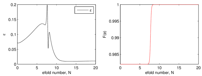
Figure 10: Evolution of the slow-roll parameter $\varepsilon$ (left) and the effective Planck mass $F$ (right) for the first $20$ $e$-folds of inflation in the two-field model. The model parameters are $m_{\chi}=5.6\times 10^{-6}$, $m_{\varphi}=4.48\times 10^{-5}$, $\beta=0.009$, $\gamma=0.111$ and $\varphi_{\ast}=1.00$, with $\chi_{\mathrm{ini}}=15.489$ and $\varphi_{\mathrm{ini}}=4.5$.

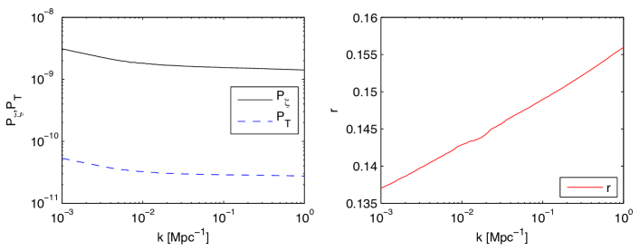
Figure 11: Power spectra (left) of scalar ($\mathcal{P}_{\zeta}$, solid black) and tensor perturbations ($\mathcal{P}_{\mathrm{T}}$, blue dashed) and the associated tensor-to-scalar ratio $r$ (right) against wavenumber $k$ (${\rm Mpc^{-1}}$) for the two-field model. The model parameters are $m_{\chi}=5.6\times 10^{-6}$, $m_{\varphi}=4.48\times 10^{-5}$, $\beta=0.009$, $\gamma=0.111$ and $\varphi_{\ast}=1.00$, with $\chi_{\mathrm{ini}}=4.5$ and $\varphi_{\mathrm{ini}}=15.489$.

IV Conclusions

We have studied the impact of sudden transitions in the effective Planck mass during inflation on primordial power spectra. In the case of single field models, we have shown that such variation gives rise to strong features in the scalar power spectra at scales corresponding to those leaving the horizon during the transition. In addition, corresponding features occur in the tensor-to-scalar ratio at the same scales. In comparison to Adams:2001vc , these features do not exhibit the oscillations that occur for step transitions in the inflationary potential itself. As shown in Sec. III, the resulting variation in the tensor-to-scalar ratio can potentially alleviate the tension between recent measurements by the Planck and BICEP2 experiments. A detailed comparison to data will be performed in future work.

Similar transitions in the Planck mass were studied in a two-field model. In this case however, sharp features are not observed in the scalar power spectrum and tensor-to-scalar ratio, as they are washed out by the conversion of isocurvature modes.

Appendix A Field equations: two-field model

In this appendix, we summarize the pertinent background field and perturbation equations for the two-field model with action comprising Eqs. (2) and (9).

The Einstein equation takes the form

$$G_{\mu\nu}=\frac{1}{F}\bigg{[}T^{(\chi)}_{\mu\nu}+\varphi_{,\mu}\varphi_{,\nu}-\frac{1}{2}g_{\mu\nu}g^{\alpha\beta}\varphi_{,\alpha}\varphi_{,\beta}+F_{;\mu\nu}-g_{\mu\nu}\Box F-g_{\mu\nu}U\bigg{]}~{},$$ (34)

where

$$T^{(\chi)}_{\mu\nu}=-\frac{2}{\sqrt{-g}}\frac{\delta S^{(\chi)}}{\delta g^{\mu\nu}}$$ (35)

is the energy-momentum tensor of the field $\chi$. Varying the full action Eq. (9) with respect to the two scalar fields yields their equations of motion:

$$2\varpi\Box\varphi\ =\ F_{,\varphi}g^{\mu\nu}T^{(\chi)}_{\mu\nu}-\varpi_{,\varphi}g^{\mu\nu}\varphi_{,\mu}\varphi_{,\nu}-4F_{,\varphi}U+2FU_{,\varphi}~{},$$ (36a)

$$\Box\chi\ =\ V_{,\chi}~{}.$$ (36b)

Lastly, the Friedmann equations take the following forms:

$$H^{2} \ =\ \frac{1}{3F}\bigg{[}\frac{1}{2}\dot{\varphi}^{2}+\frac{1}{2}\dot{\chi}^{2}+U+V-3H\dot{F}\bigg{]}~{},$$ (37a)

$$-2\dot{H} \ =\ \frac{1}{F}\bigg{[}\dot{\varphi}^{2}+\dot{\chi}^{2}+\ddot{F}-H\dot{F}\bigg{]}~{}.$$ (37b)

The relevant perturbation equations may be found in White:2012ya ; Kaiser:2010yu and are given by

$$\delta\ddot{\varphi} +\bigg{[}3H+\frac{\varpi,_{\varphi}}{\varpi}\dot{\varphi}\bigg{]}\delta\dot{\varphi}$$

$$+\bigg{[}\frac{1}{2}\bigg{(}\frac{F,_{\varphi}}{\varpi}\bigg{)}_{,\varphi}T^{(\chi)}+\frac{1}{2}\bigg{(}\frac{\varpi,_{\varphi}}{\varpi}\bigg{)}_{,\varphi}\dot{\varphi}^{2}-\frac{1}{2}\bigg{(}\frac{1}{\varpi}(4F,_{\varphi}U-2FU,_{\varphi})\bigg{)}_{,\varphi}+\frac{k^{2}}{a^{2}}\bigg{]}\delta\varphi$$

$$-(\dot{\Psi}+3\dot{\Phi})\dot{\varphi}+\frac{1}{\varpi}\bigg{[}F_{,\varphi}T^{(\chi)}-4F_{,\varphi}U+2FU_{,\varphi}\bigg{]}\Psi$$

$$+\frac{1}{2\varpi}F_{,\varphi}\delta T^{(\chi)}=0~{},$$ (38a)

$$\delta\ddot{\chi} +3H\delta\dot{\chi}+\frac{k^{2}}{a^{2}}\delta\chi-(\dot{\Psi}+3\dot{\Phi})\dot{\chi}+\,2V,_{\chi}\Psi+V,_{\chi\chi}\delta\chi=0~{}.$$ (38b)

The rhs’s of the perturbed Einstein equations (14) are given by

$$\delta\rho =\frac{1}{F}\bigg{[}\dot{\varphi}\delta\dot{\varphi}-\dot{\varphi}^{2}\Psi+\dot{\chi}\delta\dot{\chi}-\dot{\chi}^{2}\Psi+(U,_{\varphi}\delta\varphi+V,_{\chi}\delta\chi)+\,3\dot{F}(\dot{\Phi}+2H\Psi)$$

$$\qquad-3H(\delta\dot{F}+H\delta F)-\frac{k^{2}}{a^{2}}\delta F\bigg{]}~{},$$ (39a)

$$\delta q =-\frac{1}{F}\bigg{[}\dot{\varphi}\delta\varphi+\dot{\chi}\delta\chi+\delta\dot{F}-\dot{F}\Psi-H\delta F\bigg{]}~{},$$ (39b)

$$\delta p =\frac{1}{F}\bigg{[}\dot{\varphi}\delta\dot{\varphi}-\dot{\varphi}^{2}\Psi+\dot{\chi}\delta\dot{\chi}-\dot{\chi}^{2}\Psi-(U,_{\varphi}\delta\varphi+V,_{\chi}\delta\chi)-\,p_{\rm tot}\delta F+\delta\ddot{F}+2H\delta\dot{F}$$

$$\qquad-\dot{F}\dot{\Psi}-2\dot{F}\dot{\Phi}-\,2(\ddot{F}+2H\dot{F})\Psi+\frac{k^{2}}{a^{2}}\delta F\bigg{]}~{},$$ (39c)

where $p_{\mathrm{tot}}$ is the total effective pressure from the two fields. The latter is defined as

$$p_{\mathrm{tot}}=\frac{1}{F}\bigg{[}\frac{1}{2}\dot{\varphi}^{2}+\frac{1}{2}\dot{\chi}^{2}-U-V+\ddot{F}+2H\dot{F}\bigg{]}~{}.$$ (40)

Appendix B Approximate analytic solution: single-field models

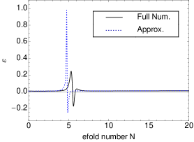
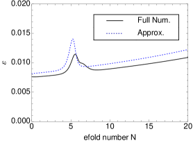
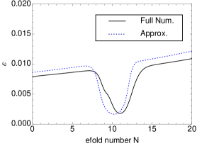
Figure 12: Comparison of the full numerical (solid black) and approximate analytic (dotted blue) solutions for the slow-roll parameter for benchmark models 1 (top left), 2 (top right) and (bottom) 3. The $e$-fold number scaling for the approximate solution was determined semi-analytically.

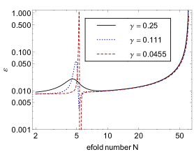
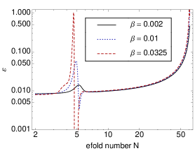
Figure 13: Approximate evolution of the slow-roll parameter $\varepsilon$ for a range of values of the parameter $\gamma$ (left, $\beta=0.01$) and $\beta$ (right, $\gamma=0.111$). The remaining model parameters were those of benchmark model 2: $m_{\varphi}=6.9\times 10^{-6}$, $\varphi_{\ast}=15.49$ and $\varphi_{\mathrm{ini}}=16.2271$.

In order to cross-check the numerical simulations and to understand the behaviour of the features in terms of variations of the parameters $\beta$ and $\gamma$, it is illustrative to obtain an approximate analytic expression for the phase diagram of the Brans-Dicke field $\varphi$ and the slow-roll parameter $\varepsilon$. By means of Eqs. (6) and (7), we may show that $\dot{\varphi}$ is given by the negative root of

$$\dot{\varphi}^{2}\ =\ \frac{1}{2A}\bigg{[}-B+\sqrt{B^{2}+4AC^{2}}\bigg{]}\;,$$ (41)

where

$$A(\varphi)\ =\ 6\bigg{(}\frac{\varpi}{F}\bigg{)}^{2}F-\varpi_{,\varphi}^{2}+3\big{(}\varpi^{2}\big{)}_{,\varphi}\bigg{(}\frac{F_{,\varphi}}{F}\bigg{)}\;,\qquad$$ (42a)

$$B(\varphi)\ =\ 12\bigg{(}\frac{\varpi}{F}\bigg{)}^{2}UF+2C\bigg{(}\varpi_{,\varphi}-3\varpi\frac{F_{,\varphi}}{F}\bigg{)}\;,\qquad$$ (42b)

$$C(\varphi)\ =\ 4F_{,\varphi}U-2FU_{,\varphi}-2\varpi\ddot{\varphi}\;.$$ (42c)

In order to find $\dot{\varphi}\equiv\dot{\varphi}(\varphi)$, we proceed iteratively under the assumption that $\ddot{\varphi}$ remains small in spite of the transient features due to transition in the effective Planck mass. In this way, we may approximate

$$C\approx C_{1}\ =\ 4F_{,\varphi}U-2FU_{,\varphi}-2\varpi\ddot{\varphi}_{1}\;,$$ (43)

with

$$\ddot{\varphi}_{1}\ =\ \frac{\mathrm{d}}{\mathrm{d}t}\dot{\varphi}_{0}\ \approx\ \dot{\varphi}_{0}\frac{\mathrm{d}}{\mathrm{d}\varphi}\dot{\varphi}_{0}\;,$$ (44)

where

$$\dot{\varphi}_{0}^{2}\ =\ \frac{1}{2A}\bigg{[}-B_{0}+\sqrt{B_{0}^{2}+4AC_{0}^{2}}\bigg{]}\;,$$ (45)

in which $C$ has been replaced throughout by

$$C_{0}\ =\ 4F_{,\varphi}U-2FU_{,\varphi}\;.$$ (46)

Figure 12 shows a comparison of the analytic approximation and full numerical results for benchmark models 1–3. We see that the shapes of the features are reproduced by the approximate solution. However, for the strong feature in benchmark model 1, the amplitude of the analytic approximation does not model well the full numerical solution. Here, we conclude that $\ddot{\varphi}/M_{\rm Pl}$ is not sufficiently small for this set of parameters for the first-order approximation detailed above to hold.

In Fig. 13, we show the evolution of the slow-roll parameter $\varepsilon$ determined using the analytic approximation above for a range of values for the parameters $\gamma$ and $\beta$. The field-dependency of the $e$-fold number $N$ was determined semi-analytically. These plots are indicative of the tuning possible for the shape of the feature in the slow-roll parameter and subsequently that occurring in the scalar power spectra $\mathcal{P}_{\zeta}$ as well as the tensor-to-scalar ratio $r$. Specifically, smaller values of $\beta$ and larger values of $\gamma$ lead to sharper and more violent features in the slow-roll parameter and therefore in the scalar power spectra. We reiterate that this first-order approximation in $\ddot{\varphi}$ only allows comparison of the shape of the feature in the slow-roll parameter. The overestimate of the amplitude noted above can also be seen from Fig. 13, in which the duration of inflation is of order $10\%$ shorter than the full numerical solutions, decreasing marginally with increasing amplitude of the feature in the slow-roll parameter.

References

- (1) S. Sarkar, Rept. Prog. Phys. 59 (1996) 1493 [hep-ph/9602260].
- (2) D. H. Lyth and A. Riotto, Phys. Rept. 314 (1999) 1 [hep-ph/9807278].
- (3) A. Liddle and D. Lyth, “Cosmological Inflation and Large-Scale Structure,” Cambridge University Press (2000).
- (4) D. Baumann and L. McAllister, [arXiv:1404.2601 [hep-th]].
- (5) G. Hinshaw et al. [WMAP Collaboration], Astrophys. J. Suppl. 208, 19 (2013) [arXiv:1212.5226 [astro-ph.CO]].
- (6) P. A. R. Ade et al. [Planck Collaboration], [arXiv:1303.5082 [astro-ph.CO]].
- (7) P. A. R. Ade et al. [BICEP2 Collaboration], Phys. Rev. Lett. 112, 241101 (2014) [arXiv:1403.3985 [astro-ph.CO]].
- (8) D. H. Lyth, Phys. Rev. Lett. 78, 1861 (1997) [hep-ph/9606387].
- (9) S. Hotchkiss, A. Mazumdar and S. Nadathur, JCAP 1202 (2012) 008 [arXiv:1110.5389 [astro-ph.CO]].
- (10) S. Antusch and D. Nolde, JCAP 1405, 035 (2014) [arXiv:1404.1821 [hep-ph]].
- (11) A. R. Liddle, A. Mazumdar and F. E. Schunck, Phys. Rev. D 58 (1998) 061301 [astro-ph/9804177].
- (12) P. Kanti and K. A. Olive, Phys. Rev. D 60 (1999) 043502 [hep-ph/9903524].
- (13) E. J. Copeland, A. Mazumdar and N. J. Nunes, Phys. Rev. D 60 (1999) 083506 [astro-ph/9904309].
- (14) A. Mazumdar, S. Panda and A. Pérez-Lorenzana, Nucl. Phys. B 614 (2001) 101 [hep-ph/0107058].
- (15) A. Jokinen and A. Mazumdar, Phys. Lett. B 597 (2004) 222 [hep-th/0406074].
- (16) K. Freese, J. A. Frieman and A. V. Olinto, Phys. Rev. Lett. 65 (1990) 3233.
- (17) F. C. Adams, J. R. Bond, K. Freese, J. A. Frieman and A. V. Olinto, Phys. Rev. D 47 (1993) 426 [hep-ph/9207245].
- (18) J. E. Kim, H. P. Nilles and M. Peloso, JCAP 0501 (2005) 005 [hep-ph/0409138].
- (19) S. Dimopoulos, S. Kachru, J. McGreevy and J. G. Wacker, JCAP 0808, 003 (2008) [hep-th/0507205].
- (20) A. Ashoorioon, H. Firouzjahi and M. M. Sheikh-Jabbari, JCAP 0906, 018 (2009) [arXiv:0903.1481 [hep-th]].
- (21) A. Ashoorioon and M. M. Sheikh-Jabbari, JCAP 1106, 014 (2011) [arXiv:1101.0048 [hep-th]].
- (22) A. Ashoorioon and M. M. Sheikh-Jabbari, [arXiv:1405.1685 [hep-th]].
- (23) E. Silverstein and A. Westphal, Phys. Rev. D 78, 106003 (2008) [arXiv:0803.3085 [hep-th]].
- (24) L. McAllister, E. Silverstein, A. Westphal and T. Wrase, [arXiv:1405.3652 [hep-th]].
- (25) A. Hebecker, S. C. Kraus and L. T. Witkowski, [arXiv:1404.3711 [hep-th]].
- (26) G. Ballesteros and J. A. Casas, [arXiv:1406.3342 [astro-ph.CO]].
- (27) Y. Wang and W. Xue, [arXiv:1403.5817 [astro-ph.CO]].
- (28) A. Ashoorioon, K. Dimopoulos, M. M. Sheikh-Jabbari and G. Shiu, [arXiv:1403.6099 [hep-th]].
- (29) J. McDonald, [arXiv:1403.6650 [astro-ph.CO]].
- (30) M. Kawasaki, T. Sekiguchi, T. Takahashi and S. Yokoyama, [arXiv:1404.2175 [astro-ph.CO]].
- (31) L. Xu, B. Chang and W. Yang, [arXiv:1404.3804 [astro-ph.CO]].
- (32) M. Bastero-Gil, A. Berera, R. O. Ramos and J. G. Rosa, [arXiv:1404.4976 [astro-ph.CO]].
- (33) Y.-F. Cai and Y. Wang, [arXiv:1404.6672 [astro-ph.CO]].
- (34) S. Mukohyama, R. Namba, M. Peloso and G. Shiu, [arXiv:1405.0346 [astro-ph.CO]].
- (35) H. Liu, P. Mertsch and S. Sarkar, [arXiv:1404.1899 [astro-ph.CO]].
- (36) M. J. Mortonson and U. Seljak, JCAP10(2014)035 [arXiv:1405.5857 [astro-ph.CO]].
- (37) R. Flauger, J. C. Hill and D. N. Spergel, [arXiv:1405.7351 [astro-ph.CO]].
- (38) V. F. Mukhanov and R. H. Brandenberger, Phys. Rev. Lett. 68 (1992) 1969.
- (39) J.-Q. Xia, Y.-F. Cai, H. Li and X. Zhang, Phys. Rev. Lett. 112 (2014) 251301 [arXiv:1403.7623 [astro-ph.CO]].
- (40) A. A. Starobinsky, JETP Lett. 55 (1992) 489 [Pisma Zh. Eksp. Teor. Fiz. 55 (1992) 477].
- (41) C. R. Contaldi, M. Peloso and L. Sorbo, JCAP 1407 (2014) 014 [arXiv:1403.4596 [astro-ph.CO]].
- (42) R. K. Jain, P. Chingangbam, J.-O. Gong, L. Sriramkumar and T. Souradeep, JCAP 0901, 009 (2009) [arXiv:0809.3915 [astro-ph]].
- (43) R. K. Jain, P. Chingangbam, L. Sriramkumar and T. Souradeep, Phys. Rev. D 82, 023509 (2010) [arXiv:0904.2518 [astro-ph.CO]].
- (44) D. K. Hazra, M. Aich, R. K. Jain, L. Sriramkumar and T. Souradeep, JCAP 1010, 008 (2010) [arXiv:1005.2175 [astro-ph.CO]].
- (45) J. A. Adams, B. Cresswell and R. Easther, Phys. Rev. D 64, 123514 (2001) [astro-ph/0102236].
- (46) M. Joy, V. Sahni and A. A. Starobinsky, Phys. Rev. D 77, 023514 (2008) [arXiv:0711.1585 [astro-ph]].
- (47) A. Ashoorioon and A. Krause, [hep-th/0607001].
- (48) A. Ashoorioon, A. Krause and K. Turzynski, JCAP 0902, 014 (2009) [arXiv:0810.4660 [hep-th]].
- (49) H. Firouzjahi and M. H. Namjoo, [arXiv:1404.2589 [astro-ph.CO]].
- (50) N. Bartolo, D. Cannone and S. Matarrese, JCAP 1310, 038 (2013) [arXiv:1307.3483 [astro-ph.CO]].
- (51) D. Battefeld, T. Battefeld, H. Firouzjahi and N. Khosravi, JCAP 1007, 009 (2010) [arXiv:1004.1417 [hep-th]].
- (52) N. Barnaby, Phys. Rev. D 82, 106009 (2010) [arXiv:1006.4615 [astro-ph.CO]].
- (53) D. Battefeld, T. Battefeld, J. T. Giblin, Jr. and E. K. Pease, JCAP 1102, 024 (2011) [arXiv:1012.1372 [astro-ph.CO]].
- (54) D. Battefeld, T. Battefeld and D. Fiene, [arXiv:1309.4082 [astro-ph.CO]].
- (55) S. Céspedes, V. Atal and G. A. Palma, JCAP 1205, 008 (2012) [arXiv:1201.4848 [hep-th]].
- (56) A. Ach carro, J. -O. Gong, G. A. Palma and S. P. Patil, Phys. Rev. D 87, no. 12, 121301 (2013) [arXiv:1211.5619 [astro-ph.CO]].
- (57) S. Céspedes and G. A. Palma, JCAP 1310, 051 (2013) [arXiv:1303.4703 [hep-th]].
- (58) R. Saito and Y. -i. Takamizu, JCAP 1306, 031 (2013) [arXiv:1303.3839 [astro-ph.CO]].
- (59) M. Konieczka, R. H. Ribeiro and K. Turzynski, JCAP 1407 (2014) 030 [arXiv:1401.6163 [astro-ph.CO]].
- (60) G. Aslanyan, L. C. Price, K. N. Abazajian and R. Easther, JCAP 08 (2014) 052 [arXiv:1403.5849 [astro-ph.CO]].
- (61) A. A. Abolhasani, H. Firouzjahi and M. Noorbala, Phys. Rev. D 86, 043522 (2012) [arXiv:1206.0903 [astro-ph.CO]].
- (62) P. A. M. Dirac, Nature 139 (1937) 323.
- (63) C. Brans and R. H. Dicke, Phys. Rev. 124 (1961) 925.
- (64) Y. Fujii, Phys. Rev. D 9 (1974) 874.
- (65) P. Minkowski, Phys. Lett. B 71 (1977) 419.
- (66) A. D. Linde, Pisma Zh. Eksp. Teor. Fiz. 30 (1979) 479 [Phys. Lett. B 93 (1980) 394].
- (67) Y. Fujii, Phys. Rev. D 26 (1982) 2580.
- (68) A. De Felice, T. Kobayashi and S. Tsujikawa, Phys. Lett. B 706 (2011) 123 [arXiv:1108.4242 [gr-qc]].
- (69) J. D. Bekenstein, Phys. Rev. D 70 (2004) 083509 [Erratum-ibid. D 71 (2005) 069901] [astro-ph/0403694].
- (70) J. D. Bekenstein and E. Sagi, Phys. Rev. D 77, 103512 (2008) [arXiv:0802.1526 [astro-ph]].
- (71) M. Milgrom, Astrophys. J. 270 (1983) 365.
- (72) Y. -S. Wu and Z. Wang, Phys. Rev. Lett. 57 (1986) 1978.
- (73) V. D. Ivashchuk and V. N. Melnikov, Nuovo Cim. B 102 (1988) 131.
- (74) V. D. Ivashchuk and V. N. Melnikov, Grav. Cosmol. 20 (2014) 26 [arXiv:1401.5491 [gr-qc]].
- (75) J. -P. Uzan, Living Rev. Rel. 14 (2011) 2 [arXiv:1009.5514 [astro-ph.CO]].
- (76) C. Wetterich, Nucl. Phys. B 302 (1988) 645.
- (77) F. S. Accetta and P. J. Steinhardt, Phys. Rev. Lett. 67, 298 (1991).
- (78) P. J. Steinhardt and C. M. Will, Phys. Rev. D 52, 628 (1995) [astro-ph/9409041].
- (79) V. F. Mukhanov, H. A. Feldman and R. H. Brandenberger, Phys. Rept. 215, 203 (1992).
- (80) J. C. Hwang and H. Noh, Phys. Rev. D 71 (2005) 063536 [gr-qc/0412126].
- (81) J. G. Williams, S. G. Turyshev and D. H. Boggs, Phys. Rev. Lett. 93, 261101 (2004) [gr-qc/0411113].
- (82) J. Muller and L. Biskupek, Class. Quant. Grav. 24 (2007) 4533.
- (83) C. J. Copi, A. N. Davis and L. M. Krauss, Phys. Rev. Lett. 92, 171301 (2004) [astro-ph/0311334].
- (84) D. I. Santiago, D. Kalligas and R. V. Wagoner, Phys. Rev. D 56 (1997) 7627 [gr-qc/9706017].
- (85) C. Bambi, M. Giannotti and F. L. Villante, Phys. Rev. D 71, 123524 (2005) [astro-ph/0503502].
- (86) A. Coc, K. A. Olive, J. -P. Uzan and E. Vangioni, Phys. Rev. D 73 (2006) 083525 [astro-ph/0601299].
- (87) N. Yunes, F. Pretorius and D. Spergel, Phys. Rev. D 81, 064018 (2010) [arXiv:0912.2724 [gr-qc]].
- (88) S. Nesseris, C. Blake, T. Davis and D. Parkinson, JCAP 1107, 037 (2011) [arXiv:1107.3659 [astro-ph.CO]].
- (89) S. Degl’Innocenti, G. Fiorentini, G. G. Raffelt, B. Ricci and A. Weiss, Astron. Astrophys. 312, 345 (1996) [astro-ph/9509090].
- (90) E. García-Berro, Y. A. Kubyshin and P. Loren-Aguilar, Int. J. Mod. Phys. D 15 (2006) 1163 [gr-qc/0512164].
- (91) S. Nesseris and L. Perivolaropoulos, Phys. Rev. D 73 (2006) 103511 [astro-ph/0602053].
- (92) E. García-Berro, P. Lorén-Aguilar, S. Torres, L. G. Althaus and J. Isern, JCAP 1105 (2011) 021 [arXiv:1105.1992 [gr-qc]].
- (93) A. H. Córsico, L. G. Althaus, E. García-Berro and A. D. Romero, JCAP 1306 (2013) 032 [arXiv:1306.1864 [astro-ph.SR]].
- (94) G. S. Bisnovatyi-Kogan, Int. J. Mod. Phys. D 15 (2006) 1047 [gr-qc/0511072].
- (95) P. Jofré, A. Reisenegger and R. Fernández, Phys. Rev. Lett. 97 (2006) 131102 [astro-ph/0606708].
- (96) J. P. W. Verbiest, M. Bailes, W. van Straten, G. B. Hobbs, R. T. Edwards, R. N. Manchester, N. D. R. Bhat and J. M. Sarkissian et al., Astrophys. J. 679 (2008) 675 [arXiv:0801.2589 [astro-ph]].
- (97) K. Lazaridis, N. Wex, A. Jessner, M. Kramer, B. W. Stappers, G. H. Janssen, G. Desvignes and M. B. Purver et al., Mon. Not. R. Astron. Soc. 400 (2009) 805 [arXiv:0908.0285 [astro-ph.GA]].
- (98) P. G. Krastev and B. -A. Li, Phys. Rev. C 76 (2007) 055804 [nucl-th/0702080 [nucl-th]].
- (99) E. Babichev, C. Deffayet and G. Esposito-Farèse, Phys. Rev. Lett. 107 (2011) 251102 [arXiv:1107.1569 [gr-qc]].
- (100) T. Chiba, N. Sugiyama and J. Yokoyama, Nucl. Phys. B 530 (1998) 304 [gr-qc/9708030].
- (101) S. Tsujikawa and H. Yajima, Phys. Rev. D 62, 123512 (2000) [hep-ph/0007351].
- (102) S. Lee, JCAP 1103 (2011) 021 [arXiv:1012.2646 [astro-ph.CO]].
- (103) R. Kimura and K. Yamamoto, JCAP 1207 (2012) 050 [arXiv:1112.4284 [astro-ph.CO]].
- (104) M. S. Turner, Phys. Rev. D 48 (1993) 3502 [astro-ph/9302013].
- (105) A. R. Liddle and S. M. Leach, Phys. Rev. D 68 (2003) 103503 [astro-ph/0305263].
- (106) D. I. Kaiser, Phys. Rev. D 52, 4295 (1995) [astro-ph/9408044].
- (107) D. I. Kaiser, [astro-ph/9507048].
- (108) T. Prokopec and J. Weenink, JCAP 1309 (2013) 027 [arXiv:1304.6737 [gr-qc]].
- (109) A. Kosowsky and M. S. Turner, Phys. Rev. D 52, 1739 (1995) [astro-ph/9504071].
- (110) S. Habib, A. Heinen, K. Heitmann and G. Jungman, Phys. Rev. D 71, 043518 (2005) [astro-ph/0501130].
- (111) P. Peter and J.-P. Uzan, Primordial cosmology, Oxford University Press, Oxford (2013).
- (112) S. Tsujikawa, D. Parkinson and B. A. Bassett, Phys. Rev. D 67, 083516 (2003) [astro-ph/0210322].
- (113) A. Ashoorioon, K. Dimopoulos, M. M. Sheikh-Jabbari and G. Shiu, JCAP 1402, 025 (2014) [arXiv:1306.4914 [hep-th]].
- (114) R. H. Ribeiro, JCAP 1205 (2012) 037 [arXiv:1202.4453 [astro-ph.CO]].
- (115) E. D. Stewart and D. H. Lyth, Phys. Lett. B 302, 171 (1993) [gr-qc/9302019].
- (116) J. M. Maldacena, JHEP 0305 (2003) 013 [astro-ph/0210603].
- (117) P. A. R. Ade et al. [Planck Collaboration], [arXiv:1303.5084 [astro-ph.CO]].
- (118) J.-c. Hwang and H. Noh, Phys. Rev. D 54 (1996) 1460.
- (119) J.-c. Hwang and H. Noh, Phys. Lett. B 506 (2001) 13 [astro-ph/0102423].
- (120) A. De Felice and S. Tsujikawa, Living Rev. Rel. 13, 3 (2010) [arXiv:1002.4928 [gr-qc]].
- (121) C. Gordon, D. Wands, B. A. Bassett and R. Maartens, Phys. Rev. D 63, 023506 (2000) [astro-ph/0009131].
- (122) J. White, M. Minamitsuji and M. Sasaki, JCAP 1207, 039 (2012) [arXiv:1205.0656 [astro-ph.CO]].
- (123) D. I. Kaiser and A. T. Todhunter, Phys. Rev. D 81, 124037 (2010) [arXiv:1004.3805 [astro-ph.CO]].