The Violation of the Taylor Hypothesis in Measurements of Solar Wind Turbulence

Abstract

Motivated by the upcoming Solar Orbiter and Solar Probe Plus missions, qualitative and quantitative predictions are made for the effects of the violation of the Taylor hypothesis on the magnetic energy frequency spectrum measured in the near-Sun environment. The synthetic spacecraft data method is used to predict observational signatures of the violation for critically balanced Alfvénic turbulence or parallel fast/whistler turbulence. The violation of the Taylor hypothesis can occur in the slow flow regime, leading to a shift of the entire spectrum to higher frequencies, or in the dispersive regime, in which the dissipation range spectrum flattens at high frequencies. It is found that Alfvénic turbulence will not significantly violate the Taylor hypothesis, but whistler turbulence will. The flattening of the frequency spectrum is therefore a key observational signature for fast/whistler turbulence.

1. Introduction

The turbulent cascade of energy from large to small scales influences plasma evolution and heating in many astrophysical environments, from galaxy clusters and accretion disks to the solar corona and solar wind. Extensive in situ observations of the near-Earth solar wind provide invaluable opportunities to test theories of turbulent transport, dissipation, and heating. Upcoming missions, including Solar Orbiter and Solar Probe Plus, will make the first in situ measurements of turbulence in the near-Sun environment, providing crucial data to identify the mechanisms governing coronal heating.

The interpretation of in situ measurements of plasma turbulence is complicated by the fact that the turbulence is measured in a frame of reference (the spacecraft frame) that is in relative motion with respect to the frame of reference of the solar wind plasma (the plasma frame). For a spatial Fourier mode with wavevector $\mathbf{k}$, the transformation from the frequency $\omega$ in the plasma frame to the observed frequency $\omega_{sc}$ in the spacecraft frame yields the relation

$$\omega_{sc}=\omega+\mathbf{k}\cdot\mathbf{v}_{sw},$$ (1)

(Taylor, 1938); a derivation can be found in a companion work, Howes et al. (2014b), heretofore referred to as Paper I. For a turbulent distribution of modes in wavevector space, the plasma-frame frequency term $\omega$ and spatial advection term $\mathbf{k}\cdot\mathbf{v}_{sw}$, both contributing to the spacecraft-frame frequency, cannot be uniquely separated using single-point spacecraft measurements.

The typically super-Alfvénic velocity of the solar wind near Earth, $v_{sw}\gg v_{A}$, motivates the use of the Taylor hypothesis (Taylor, 1938; Fredricks & Coroniti, 1976), assuming that $|\omega|\ll|\mathbf{k}\cdot\mathbf{v}_{sw}|$, thereby relating the spacecraft-frame frequency directly to the wavenumber of spatial fluctuations, $\omega_{sc}\simeq\mathbf{k}\cdot\mathbf{v}_{sw}$. When the plasma-frame frequency is non-negligible, $|\omega|\gtrsim|\mathbf{k}\cdot\mathbf{v}_{sw}|$, the Taylor hypothesis is violated. A number of previous studies have addressed this issue in the context of different analyses of solar wind measurements (Fredricks & Coroniti, 1976; Matthaeus & Goldstein, 1982; Goldstein et al., 1986; Leamon et al., 1998; Jian et al., 2009; Perri & Balogh, 2010). In Paper I (Howes et al 2014b), analytic expressions for the validity of the Taylor hypothesis are derived for plasma waves relevant to solar wind turbulence. In this letter, we aim to determine the qualitative and quantitative effects of the violation of the Taylor hypothesis on the magnetic energy frequency spectrum in the solar wind, and in doing so validate expressions derived in Paper I.

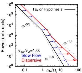
Figure 1.— Model of the magnetic energy spectrum vs. normalized frequency, $\omega_{*}/\Omega_{i}=(\omega_{sc}/\Omega_{i})/(v_{sw}/v_{A})$, for a turbulent distribution of whistler waves with $v_{sw}/v_{A}=1$, illustrating the mapping of the wavenumber spectrum (Taylor hypothesis, black) to the measured frequency spectrum. Violation of the Taylor hypothesis for slow flow leads to constant shift to higher frequency (blue arrows) of the entire spectrum. At high frequency, the dispersive nature of the whistler waves leads to a flattening of the frequency spectrum (red arrows).

To explore the violation of the Taylor hypothesis for turbulence measurements in the solar wind requires an estimate of the plasma-frame frequency of the turbulent fluctuations. We assume that the frequency of the turbulent fluctuations is well characterized by the frequency of the linear waves supported by the solar wind plasma (TenBarge & Howes, 2012). This assumption of linear wave frequencies is one element of a broader approach to the modeling of plasma turbulence called the quasilinear premise; a discussion of this approach, including supporting evidence, is presented in Klein et al. (2012) and Howes et al. (2014a). Note that the study presented here depends only on the less stringent requirement that the linear wave frequency is a good measure of the maximum frequency of turbulent fluctuations. In the weakly collisional conditions of the solar wind plasma, we explore models in which the turbulent fluctuations in the dissipation range are a broadband spectrum of either kinetic Alfvén waves or whistler waves, as suggested from a variety of turbulence theories (Goldreich & Sridhar, 1995; Stawicki et al., 2001; Galtier, 2006; Boldyrev, 2006; Schekochihin et al., 2009), numerical simulations (Howes et al., 2008b; Saito et al., 2008; Parashar et al., 2009; Gary et al., 2012; TenBarge & Howes, 2012), and solar wind observations (Bale et al., 2005; Sahraoui et al., 2010; Salem et al., 2012; Chen et al., 2013).

In this Letter, we predict effects of the violation of the Taylor hypothesis on Solar Probe Plus measurements of the magnetic energy spectrum as a function of the ratio of solar wind velocity to Alfvén velocity, $\overline{V}\equiv v_{sw}/v_{A}$. Both the synthetic spacecraft data method and a simplified analytical model are used to predict the mapping of a given wavenumber spectrum of the turbulence to a measured frequency spectrum.

As illustrated in Fig. 1, the Taylor hypothesis is violated in two regimes: the slow flow regime and the dispersive regime. In the slow flow regime, the solar wind flow is slow enough that the plasma frame-frequency term is non-negligible compared to the advection term, $|\omega|\gtrsim|\mathbf{k}\cdot\mathbf{v}_{sw}|$, leading to a constant shift of the spacecraft-frame frequency spectrum to higher frequency (blue arrows), without altering the scaling of the spectrum. In the dispersive regime, the plasma-frame frequency increases more rapidly than linearly with the wavenumber, but the advection term only increases linearly, so the plasma-frame frequency term will eventually dominate the spacecraft-frame frequency, leading to a flattening of the magnetic energy spectrum (red arrows). This applies to a turbulent spectrum of kinetic Alfvén waves or whistler waves, but the anisotropic distribution of turbulent power in wavevector space plays an important role in distinguishing these two cases. A complete explanation of Fig. 1 is deferred to the discussion section below.

2. Synthetic Spacecraft Data Method

To determine the impact of the plasma-frame frequency on the observed magnetic energy frequency spectrum, we generate time series using the synthetic spacecraft data method (Klein et al., 2012). Adopting the quasilinear premise, this method models the turbulence as a spectrum of randomly-phased, linear kinetic wave modes. By sampling along a trajectory through the synthetic plasma volume, we create single-point time series that may undergo the same analysis as in situ measurements. First- and second-order correlations in the turbulence, including energy spectra, can be modeled using these synthetic time series and are found to be in good agreement with solar wind observations (Howes et al., 2012; Klein et al., 2012; TenBarge et al., 2012; Klein et al., 2014), but since the nonlinear interactions responsible for the turbulent energy transfer between modes are not modeled, such synthetic time series cannot be used to study third- or higher-order correlations.

To create the synthetic data, the magnetic field is calculated as a time series along a defined trajectory $\mathbf{r}(t)=-\mathbf{v}_{sw}t$ in the plasma volume according to eq. (3) from Paper I

$$\mathbf{B}(t)=\sum_{m}\sum_{\mathbf{k}}\hat{\mathbf{B}}_{m}(\mathbf{k})e^{-i[\mathbf{k}\cdot\mathbf{v}_{sw}+\omega_{m}(\mathbf{k})]t},$$ (2)

where $\omega_{m}(\mathbf{k})$ is the linear eigenfrequency for wave mode $m$ with wavevector $\mathbf{k}$, and $\hat{\mathbf{B}}_{m}(\mathbf{k})$ is the corresponding complex Fourier coefficient, each of which is multiplied by a random phase $\exp(i\eta_{\mathbf{k},m})$.

In this Letter, the synthetic data is generated on a cubic wavevector grid with $512^{3}$ points, spanning one of two ranges: the inertial range $0.01\leq|k_{j}\rho_{i}|\leq 2.56$, or the transition range $0.1\leq|k_{j}\rho_{i}|\leq 25.6$, where $\rho_{i}$ is the ion gyroradius and the index $j$ signifies $x$, $y$, or $z$. The frequencies and eigenfunctions for the linear kinetic wave modes are calculated numerically for each wavevector using the linear Vlasov-Maxwell dispersion relation (Quataert, 1998; Howes et al., 2006). The fully ionized, proton-electron plasma is assumed to have an isotropic, non-relativistic Maxwellian velocity distribution with a realistic mass ratio, $m_{i}/m_{e}=1836$, and equal ion and electron temperatures. We choose the ion plasma beta $\beta_{i}=8\pi n_{i}T_{i}/B^{2}=1$, so the ion gyroradius and ion inertial length are equal, $d_{i}=\rho_{i}/\sqrt{\beta_{i}}$

We study the violation of the Taylor hypothesis for two turbulence models: (i) critically balanced Alfvénic turbulence, or (ii) parallel fast/whistler turbulence. For the Alfvénic case, only wavevectors at or below critical balance, $k_{\parallel}B_{0}\lesssim k_{\perp}\delta B_{\perp}$, (Goldreich & Sridhar, 1995; Howes et al., 2008a, 2011; TenBarge & Howes, 2012) are nonzero; for the fast/whistler case, only wavevectors at an angle $\leq 45^{\circ}$ with respect to the mean magnetic field $\mathbf{B}_{0}$ are nonzero. The distribution of power is axisymmetric about $\mathbf{B}_{0}$, with amplitudes chosen to yield a one-dimensional magnetic energy spectrum breaking from $k^{-5/3}$ to $k^{-2.8}$ at $k\rho_{i}=1$, consistent with observations (Alexandrova et al., 2008; Podesta, 2009; Sahraoui et al., 2009). Variation of these spectral indices within observational constraints does not significantly impact our findings.

The synthetic time series are sampled on a $45^{\circ}$ trajectory with respect to $\mathbf{B}_{0}$. For each turbulence model and wavevector range, we choose five values of $\overline{V}\in[10.0,3.0,1.0,0.3,0.1]$ to model conditions in both the near-Earth solar wind and solar corona, constructing an ensemble of $64$ time series with independent random phases $\eta_{\mathbf{k},m}$ for each case. A Taylor hypothesis case is also computed with $\omega_{m}(\mathbf{k})=0$ in eq. (2). The magnetic energy frequency spectrum is calculated for each time series and then ensemble averaged. These averages are shown in Figs. 2 and 3, with the spectra of the inertial and transition ranges overlaid.

3. Results

In Fig. 2, the magnetic energy spectra for the five $\overline{V}$ cases (colors) are compared to the Taylor hypothesis case (black). In Fig. 3, each $\overline{V}$ case is offset vertically for individual comparison to the Taylor hypothesis case (grey, same vertical offsets), with inertial range (blue) and transition range (red) results distinguished.

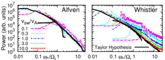
Figure 2.— Averaged magnetic energy spectra from an ensemble of synthetic spacecraft data generated from critically balanced Alfvénic (left) or parallel fast/whistler (right) turbulence for 5 values of $\overline{V}$ (colors) and the Taylor hypothesis case (black). Inertial and transition range results are overlaid.

To facilitate the comparison between frequency spectra with differing values of $\overline{V}$, we adopt the normalization $\omega_{*}/\Omega_{i}\equiv(\omega_{sc}/\Omega_{i})/\overline{V}$, which transforms eq. (1) to

$$\omega_{*}/\Omega_{i}=(\omega/\Omega_{i})/\overline{V}+kd_{i}\cos\theta,$$ (3)

where $\mathbf{k}\cdot\mathbf{v}_{sw}=kv_{sw}\cos\theta$. This transformation puts the $\overline{V}$ dependence into the plasma-frame frequency term, so any difference between the Taylor hypothesis case and a finite $\overline{V}$ case is due to a violation of the Taylor hypothesis.

The primary qualitative results of this Letter are apparent in Figs. 2 and 3. For the critically balanced Alfvénic turbulence (left panels), there is no significant violation of the Taylor hypothesis for flow velocity ratios $\overline{V}\geq 0.3$. For the parallel fast/whistler turbulence, the Taylor hypothesis is violated significantly for all values of $\overline{V}$. These results confirm the analytical predictions in Paper I. The spacecraft-frame frequency spectrum for the case of parallel fast/whistler turbulence is modified qualitatively by two distinct effects.

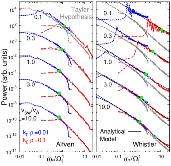
Figure 3.— The same spectra shown in Fig. 2 offset vertically to highlight deviation of each case from the Taylor hypothesis case (grey). Inertial (blue dash) and transition (red dot-dash) ranges are shown. In the right panel, the analytical model (black solid) is plotted, along with the break (green circle) and critical (cyan triangle) frequencies.

The first effect is a shift of the entire spectrum from the Taylor hypothesis case to higher frequency, seen for $\overline{V}\leq 1$. This effect is due to the slow flow of the solar wind with respect to the Alfvén velocity, $v_{sw}\lesssim v_{A}$. The non-negligible contribution from the plasma-frame frequency in eq. (1) leads to this constant shift at all frequencies and is highlighted by a shift to the right of the break frequency, $\omega_{b*}$ (green circle in Fig. 3). In contrast, for critically balanced Alfvénic turbulence, there is not a significant shift in $\omega_{b*}$ for any value of $\overline{V}$.

The second effect is the flattening of the spectrum at high frequency, most easily seen in the right panels of Figs. 2 and 3 as $\overline{V}$ decreases. This effect is due to the dispersive nature of whistler waves at $kd_{i}\gtrsim 1$, leading to a more rapid than linear increase of plasma-frame frequency with increasing wavenumber. Since the spatial advection term scales linearly with wavenumber, even for rapid solar wind flow, eventually the plasma-frame frequency term will become non-negligible due to its more rapid increase with wavenumber. This dispersive increase of the wave frequency flattens the frequency spectrum for frequencies higher than a critical frequency, $\omega_{c*}$ (cyan triangle in Fig. 3), although this transition is often gradual.

Several other minor features are apparent in Figs. 2 and 3. First, the pronounced peaks in the low $\overline{V}$ cases are an artifact caused by the discrete nature of our wavevector grid at the largest scales. Second, the contribution from the plasma-frame frequency shifts power to higher frequencies, causing a small but noticeable aliasing at the high-frequency end of the spectra as more power is shifted above the Nyquist frequency of the synthetic time series. Finally, small bumps in the spectra for the Alfvénic cases with $\overline{V}\leq 0.3$ at $\omega_{*}/\Omega_{i}\sim 10$ are due to a mode transition from kinetic Alfvén waves to ion Bernstein waves in our turbulent power distribution at $k_{\perp}\rho_{i}\simeq 7$.

4. Analytical Model

To illuminate the effect of the violation of the Taylor hypothesis, we construct a simple analytical model that reproduces the two primary qualitative effects in the slow flow and dispersive regimes. Here we present only the model for the parallel fast/whistler turbulence.

For a given piecewise-continuous, magnetic energy wavenumber spectrum $E(k)=(E_{0}/k_{0})(kd_{i})^{-5/3}$ at $kd_{i}<1$ and $E(k)=(E_{0}/k_{0})(kd_{i})^{-2.8}$ at $kd_{i}\geq 1$, the problem boils down to finding a mapping $k(\omega_{sc})$ so that we may determine the frequency spectrum $E(\omega_{sc})=E[k(\omega_{sc})]$. Here $k_{0}$ is the outer scale wavenumber and $E_{0}$ is a constant to adjust the total turbulent magnetic energy. The fast/whistler wave dispersion relation is expressed by $\omega=kv_{A}\sqrt{1+(k_{\parallel}di)^{2}}$ in Paper I.

The key simplification needed to obtain an analytical solution is to find the mapping $k(\omega_{sc})$ along a particular 1D path through 3D wavevector space. We choose the path $k_{\perp}=k_{\parallel}$, and we sample at velocity $\mathbf{v}_{sw}$ along this path at a $45^{\circ}$ angle with respect to $\mathbf{B}_{0}$; in this case, $\theta=0$, so $\mathbf{k}\cdot\mathbf{v}_{sw}=kv_{sw}$. Although this choice may seem to limit the generality of the solution, the steeply dropping energy spectrum is dominated by the largest frequency associated with a particular wavevector amplitude $k$; the case $\theta=0$ gives the maximum frequency from the advection term for a given $k$, and therefore this is the dominant contribution. Along this path, eq. (3) becomes

$$\omega_{*}/\Omega_{i}=kd_{i}\left[1+\sqrt{1+(1/2)(kd_{i})^{2}}/\overline{V}\right].$$ (4)

We convert this function into the piecewise function $\omega_{*}/\Omega_{i}=kd_{i}(1+1/\overline{V})$ for $kd_{i}<\sqrt{2}$ and $\omega_{*}/\Omega_{i}=kd_{i}[1+kd_{i}/(\overline{V}\sqrt{2})]$ for $kd_{i}\geq\sqrt{2}$. This piecewise function may be easily inverted to yield,

$$kd_{i}=\left\{\begin{array}[]{lc}\frac{\omega_{*}}{\Omega_{i}}\frac{\overline{V}}{1+\overline{V}},&\frac{\omega_{*}}{\Omega_{i}}<\sqrt{2}(1+\frac{1}{\overline{V}})\\ -\frac{\overline{V}}{\sqrt{2}}+\sqrt{\frac{\overline{V}^{2}}{2}+\sqrt{2}\frac{\omega_{*}}{\Omega_{i}}\overline{V}},&\frac{\omega_{*}}{\Omega_{i}}\geq\sqrt{2}(1+\frac{1}{\overline{V}}).\end{array}\right.$$ (5)

Using this function for $k(\omega_{*})$, we can immediately plot the frequency spectrum $E(\omega_{*})$, shown as the solid black lines in the right panel of Fig. 3. This simple analytical model agrees well with the frequency spectra generated by the synthetic spacecraft data method at all values of $\overline{V}$. In addition, the model may be used to obtain analytical estimates for the break frequency $\omega_{b*}$ and the critical frequency $\omega_{c*}$. The break frequency for our model occurs at $kd_{i}=1$, so we obtain $\omega_{b*}/\Omega_{i}=1+1/\overline{V}$, given by the green circles in Fig. 3. The critical frequency, where dispersive effects become significant, requires both the waves to be dispersive and the plasma-frame frequency term to be significant (taken to be $|\omega|\geq|\mathbf{k}\cdot\mathbf{v}_{sw}|/3$). This concurrence occurs at $kd_{i}=\sqrt{2}\max[1,((\overline{V}/3)^{2}-1)^{1/2}]$ and leads to a prediction for the critical frequency of $\omega_{c*}/\Omega_{i}=\sqrt{2}(1+1/\overline{V})$ for $\overline{V}\leq 3\sqrt{2}$ and $\omega_{c*}/\Omega_{i}=\sqrt{2}[((\overline{V}/3)^{2}-1)^{1/2}+((\overline{V}/3)^{2}-1)/\overline{V}]$ for $\overline{V}>3\sqrt{2}$, indicated by cyan triangles in Fig. 3.

5. Discussion

We can use this analytical model to predict quantitatively the effect of the violation of the Taylor hypothesis on the magnetic energy frequency spectrum, as depicted in Fig. 1. The violation in the slow flow regime is easily calculated in the limit $kd_{i}\ll 1$, simplifying eq. (4) to $\omega_{*}/\Omega_{i}\simeq kd_{i}(1+1/\overline{V})$. Since the scaling of $\omega_{*}$ is the same as $k$, the spectrum will have the same scaling but will be shifted to higher frequency by a factor $(1+1/\overline{V})$, as depicted by the blue arrows in Fig. 1. To highlight this effect for non-dispersive waves, we apply this result to an artificial fast/whistler dispersion relation that has no dispersion, $\omega/\Omega_{i}=kd_{i}$ (blue dot-dash).

To calculate the violation of the Taylor hypothesis in the dispersive regime, we simplify eq. (4) in the limit $kd_{i}\gg 1$ to $\omega_{*}/\Omega_{i}\simeq kd_{i}[1+kd_{i}/(\overline{V}\sqrt{2})]$. When $kd_{i}\gg\overline{V}\sqrt{2}$, the plasma-frame frequency term dominates due to the more rapid than linear increase of whistler wave frequency with wavenumber, $\omega/\Omega_{i}=kd_{i}\sqrt{1+(kd_{i})^{2}/2}$, giving $\omega_{*}/\Omega_{i}\simeq(kd_{i})^{2}/(\overline{V}\sqrt{2})$. Therefore, we obtain a mapping $k\propto\omega_{*}^{1/2}$, leading to a flattening of the frequency spectrum to $E(k)\propto k^{-2.8}\propto\omega_{*}^{-1.4}$, as indicated by the red arrows in Fig. 1. Note, however, that the onset of this flattening can be gradual, only reaching $E(k)\propto\omega_{sc}^{-1.4}$ at $kd_{i}\gg\overline{V}\sqrt{2}$, as seen in Fig. 1.

To highlight further the features of the model and to compare to the synthetic spacecraft data results, we plot compensated spectra in Fig. 4. The magnetic energy frequency spectra produced from the inertial range (blue) and transition range (red) are compensated by $\omega^{1.7}_{*}$ and $\omega^{2.8}_{*}$, respectively. For three parallel fast/whistler cases with $\overline{V}=10.0,1.0,0.3$, (counter-clockwise from lower right) the compensated energy spectra are flat up to $\omega_{c*}$, and steepen at higher frequencies. The values for $\omega_{b*}$ and $\omega_{c*}$ calculated from the model correspond well with the breaks seen in the compensated synthetic energy spectra. The strong correspondence between the one-dimensional analytic model and the three-dimensional synthetic spacecraft results serve as a posteriori support for the approximations used in the analytic model.

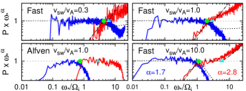
Figure 4.— Compensated magnetic energy spectra from four synthetic data sets generated for Alfvénic turbulence with $\overline{V}=1.0$ (lower left) and fast/whistler turbulence with $\overline{V}=10.0,\ 1.0,\ 0.3$ (counter-clockwise from lower right). Spectra from the inertial and transition ranges are compensated by $\omega_{*}^{1.7}$ (blue) and $\omega_{*}^{2.8}$ (red). Also plotted are the analytical model compensated by $\omega_{*}^{1.7}$ (black dash) and $\omega_{*}^{2.8}$ (black dot-dash), as well as $\omega_{b*}$ (green circle) and $\omega_{c*}$ (cyan triangle).

Note that synthetic time series with $\beta_{i}\ll 1$ (not shown here), relevant to the near-Sun environment, have been found to have qualitatively similar spectral features to those described here.

6. Conclusions

In this Letter, we determine the qualitative and quantitative effects on the measured magnetic energy frequency spectrum in the solar wind due to the violation of the Taylor hypothesis. For upcoming spacecraft missions, such as Solar Probe Plus, we find the Taylor hypothesis may be violated in two regimes: the slow flow and dispersive regimes. In the slow flow regime, a significant plasma-frame frequency contribution to the spacecraft-frame frequency leads to a shift of the frequency spectrum to higher frequency by a factor $1+v_{A}/v_{sw}$ relative to a Taylor hypothesis case where $\omega_{sc}=\mathbf{k}\cdot\mathbf{v}_{sw}$ but no change in the scaling of the spectrum. Since the underlying wavevector spectrum cannot be determined by a single spacecraft, this effect is undetectable. In the dispersive regime, the dispersive increase of wave frequency with wavenumber, $\omega\propto k^{2}$, can lead to a flattening of the typical dissipation range $k^{-2.8}$ wavenumber spectrum to an $\omega^{-1.4}$ frequency spectrum. We confirm earlier predictions from Paper I that critically balanced Alfvénic turbulence will not, but parallel fast/whistler turbulence will, significantly violate the Taylor hypothesis, especially near the Alfvén critical point where $v_{sw}\sim v_{A}$. Thus, a flattening of the frequency spectrum in the dissipation range is the predicted observational signature for fast/whistler turbulence. For Solar Probe Plus measurements, the shifting of power to higher frequencies may also threaten to cause significant aliasing of measured signals, even at the high sampling rate of the instruments.

This work was supported by NSF CAREER AGS-1054061 and NASA NNX10AC91G.

References

- Alexandrova et al. (2008) Alexandrova, O., Carbone, V., Veltri, P., & Sorriso-Valvo, L. 2008, ApJ, 674, 1153
- Bale et al. (2005) Bale, S. D., Kellogg, P. J., Mozer, F. S., Horbury, T. S., & Reme, H. 2005, PhRvL, 94, 215002
- Boldyrev (2006) Boldyrev, S. 2006, PhRvL, 96, 115002
- Chen et al. (2013) Chen, C. H. K., Boldyrev, S., Xia, Q., & Perez, J. C. 2013, PhRvL, 110, 225002
- Fredricks & Coroniti (1976) Fredricks, R. W., & Coroniti, F. V. 1976, JGR, 81, 5591
- Galtier (2006) Galtier, S. 2006, JPlPh, 72, 721
- Gary et al. (2012) Gary, S. P., Chang, O., & Wang, J. 2012, ApJ, 755, 142
- Goldreich & Sridhar (1995) Goldreich, P., & Sridhar, S. 1995, ApJ, 438, 763
- Goldstein et al. (1986) Goldstein, M. L., Roberts, D. A., & Matthaeus, W. H. 1986, JGR, 91, 13357
- Howes et al. (2012) Howes, G. G., Bale, S. D., Klein, K. G., et al. 2012, ApJL, 753, L19
- Howes et al. (2006) Howes, G. G., Cowley, S. C., Dorland, W., et al. 2006, ApJ, 651, 590
- Howes et al. (2008a) —. 2008a, JGR, 113, 5103
- Howes et al. (2008b) Howes, G. G., Dorland, W., Cowley, S. C., et al. 2008b, PhRvL, 100, 065004
- Howes et al. (2014a) Howes, G. G., Klein, K. G., & TenBarge, J. M. 2014a, arXiv:1404.2913
- Howes et al. (2014b) —. 2014b, ApJ, 789, 106
- Howes et al. (2011) Howes, G. G., Tenbarge, J. M., & Dorland, W. 2011, PhPl, 18, 102305
- Jian et al. (2009) Jian, L. K., Russell, C. T., Luhmann, J. G., et al. 2009, ApL, 701, L105
- Klein et al. (2012) Klein, K. G., Howes, G. G., TenBarge, J. M., et al. 2012, ApJ, 755, 159
- Klein et al. (2014) Klein, K. G., Howes, G. G., TenBarge, J. M., & Podesta, J. J. 2014, ApJ, 785, 138
- Leamon et al. (1998) Leamon, R. J., Smith, C. W., Ness, N. F., Matthaeus, W. H., & Wong, H. K. 1998, JGR, 103, 4775
- Matthaeus & Goldstein (1982) Matthaeus, W. H., & Goldstein, M. L. 1982, JGR, 87, 6011
- Parashar et al. (2009) Parashar, T. N., Shay, M. A., Cassak, P. A., & Matthaeus, W. H. 2009, PhPl, 16, 032310
- Perri & Balogh (2010) Perri, S., & Balogh, A. 2010, ApJ, 714, 937
- Podesta (2009) Podesta, J. J. 2009, ApJ, 698, 986
- Quataert (1998) Quataert, E. 1998, ApJ, 500, 978
- Sahraoui et al. (2010) Sahraoui, F., Goldstein, M. L., Belmont, G., Canu, P., & Rezeau, L. 2010, PhRvL, 105, 131101
- Sahraoui et al. (2009) Sahraoui, F., Goldstein, M. L., Robert, P., & Khotyaintsev, Y. V. 2009, PhRvL, 102, 231102
- Saito et al. (2008) Saito, S., Gary, S. P., Li, H., & Narita, Y. 2008, PhPl, 15, 102305
- Salem et al. (2012) Salem, C. S., Howes, G. G., Sundkvist, D., et al. 2012, ApL, 745, L9
- Schekochihin et al. (2009) Schekochihin, A. A., Cowley, S. C., Dorland, W., et al. 2009, ApJS, 182, 310
- Stawicki et al. (2001) Stawicki, O., Gary, S. P., & Li, H. 2001, JGR, 106, 8273
- Taylor (1938) Taylor, G. I. 1938, RSPSA, 164, 476
- TenBarge & Howes (2012) TenBarge, J. M., & Howes, G. G. 2012, PhPl, 19, 055901
- TenBarge et al. (2012) TenBarge, J. M., Podesta, J. J., Klein, K. G., & Howes, G. G. 2012, ApJ, 753, 107