Entanglement negativity in the harmonic chain out of equilibrium

Abstract

We study the entanglement in a chain of harmonic oscillators driven out of equilibrium by preparing the two sides of the system at different temperatures, and subsequently joining them together. The steady state is constructed explicitly and the logarithmic negativity is calculated between two adjacent segments of the chain. We find that, for low temperatures, the steady-state entanglement is a sum of contributions pertaining to left- and right-moving excitations emitted from the two reservoirs. In turn, the steady-state entanglement is a simple average of the Gibbs-state values and thus its scaling can be obtained from conformal field theory. A similar averaging behaviour is observed during the entire time evolution. As a particular case, we also discuss a local quench where both sides of the chain are initialized in their respective ground states.

1 Introduction

In the last decade it has been recognized that the entanglement content of many-body quantum states carries essential information about the underlying system [1, 2]. In the simplest case, when the system is in a pure state, the entanglement between two complementary parts is measured by the entanglement entropy. One of the most remarkable results for the case of one-dimensional systems is that the entanglement entropy of ground states displays a universal behaviour. At critical points it grows logarithmically in the subsystem size [3], with a prefactor governed by the central charge of the underlying conformal field theory (CFT) [4]; while for noncritical chains it saturates to a finite value, i.e., an area law holds [5].

However, the use of the entropy as an entanglement measure is restricted to pure states and a bipartite setting. The entanglement between non-complementary subsystems, embedded in a larger system, thus needs a different characterization, since the reduced state is in general mixed. Among the numerous proposals to quantify mixed-state entanglement [6], the logarithmic negativity [7, 8] turns out to be a particularly useful and easily computable measure. It is especially simple to evaluate for coupled harmonic oscillators [9] and in general for Gaussian states of continuous variable systems [10]. In particular, the logarithmic negativity was used to characterize tripartite entanglement in the ground state of the one-dimensional harmonic chain [11]. Furthermore, results obtained for various quantum spin chains [12, 13] indicate universal features in the entanglement of disjoint intervals at criticality. These universal features have recently been understood via CFT methods [14, 15]; the corresponding analytical predictions have been compared to numerical simulations in various 1D critical systems [16, 17, 18] and a very good agreement was found. In two dimensions, entanglement negativity has also been shown to detect topological order [19, 20].

In spite of this renewed interest, the behaviour of the entanglement negativity has not yet been investigated out of equilibrium. Here we consider such a problem for a chain of harmonic oscillators that is released from an initial state where the two sides of the chain are kept at different temperatures. The system driven by this thermal gradient evolves, for long times, into a nonequilibrium steady state (NESS) carrying a constant flux of energy. In the gapless limit of the harmonic chain and for sufficiently low reservoir temperatures, the NESS is believed to be described by a nonequilibrium CFT with universal behaviour for e.g. the energy flow [21, 22] and thus one expects that universal signatures may also appear in the entanglement negativity.

The choice of our nonequlibrium setup is further motivated by recent studies of a free-fermion chain where the same type of NESS was shown to violate the area law for the mutual information [23]. Similar logarithmic violations were found for the XY spin chain [24] which shows a marked contrast to the thermal-state behaviour where a strict area law can be proven to hold [25]. Since the mutual information measures only the total (classical + quantum) correlations between subsystems, it is natural to ask whether such a singular behaviour would be present for the steady-state entanglement negativity. The NESS of the harmonic chain is an ideal candidate to attack this question since, in contrast to free fermions or spin chains, the logarithmic negativity can easily be extracted from the covariance matrix [9].

Here we focus on the entanglement between adjacent segments of the chain and in a low-temperature limit of the NESS. Our main result is to show that the logarithmic negativity is, to a very good approximation, a sum of two contributions from left- and right-moving normal-mode excitations emitted from the reservoirs. They both carry one-half of the corresponding thermal-state entanglement that can be found from a simple generalization of the ground-state CFT calculations [14, 15]. Hence the steady-state entanglement of the harmonic chain obeys a strict area law.

In the next section we define the model and describe the initial and time evolved states, which is followed by a discussion of the steady state properties for the infinite chain in Sec. 3. Next, we present the covariance matrix formalism in Sec. 4 that is used to obtain the logarithmic negativity. The method is then applied to calculate the steady-state entanglement in Sec. 5 whereas the full time evolution starting from the initial state is presented in Sec. 6. The results are discussed in Sec. 7 and some details of the calculations are presented in two Appendices.

2 Model and setting

The Hamiltonian of the harmonic chain of length $N$ (with units $m=\hbar=1$) is given by

$$H=\frac{1}{2}\sum_{n=0}^{N}\left[p_{n}^{2}+K({x}_{n+1}-{x}_{n})^{2}+\omega_{0}^{2}x_{n}^{2}\right],$$ (1)

where $x_{n}$ and $p_{n}$ denote the position and momentum operators of the $n$-th oscillator with canonical commutation relations $\left[x_{m},p_{n}\right]=i\delta_{m,n}$ and $\left[x_{m},x_{n}\right]=\left[p_{m},p_{n}\right]=0$. The parameters $K$ and $\omega_{0}^{2}$ set the strength of the nearest neighbour coupling and the external harmonic confining potential at each site, respectively. On the chain ends we impose Dirichlet boundary conditions (fixed walls) which imply $x_{0}=x_{N+1}=0$ and $p_{0}=p_{N+1}=0$.

The initial state is given by a simple product of Gibbs states

$$\rho(0)=\frac{1}{Z_{l}}\mathrm{e}^{-\beta_{l}H_{l}}\otimes\frac{1}{Z_{r}}\mathrm{e}^{-\beta_{r}H_{r}}\,,$$ (2)

with inverse temperatures $\beta_{l}$ and $\beta_{r}$ for the left and right half-chains, respectively. The Hamiltonian $H_{l}$ ($H_{r}$) is defined by a similar expression as in Eq. (1) with the limits of the sum given by $0,N/2$ ($N/2,N$) and Dirichlet boundary conditions imposed at sites $0$ and $N/2+1$ ($N/2$ and $N+1$). The initially disconnected halves are joined together at time $t=0$ and the state evolves unitarily $\rho(t)=\mathrm{e}^{-iHt}\rho(0)\mathrm{e}^{iHt}$ under the action of Hamiltonian (1). The change in the geometry of the chain is depicted in Fig. 1.

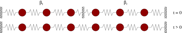
Figure 1: Geometry of the oscillator chain before and after the quench.

Since both the initial state as well as the time evolution operator is Gaussian, $\rho(t)$ can be fully characterized by its $2N\times 2N$ covariance matrix $C(t)$. This can be written in a block-matrix form, composed of symmetric $2\times 2$ matrices

$$C_{m,n}(t)=\langle R_{m}(t)R^{T}_{n}(t)+R_{n}(t)R^{T}_{m}(t)\rangle,\quad R_{n}(t)=\left(\begin{array}[]{c}x_{n}(t)\\ p_{n}(t)\end{array}\right),$$ (3)

where $R_{n}(t)$ is a vector of the position and momentum operators in the Heisenberg picture at site $n$, and $\langle\mathcal{O}(t)\rangle=\Tr\left[\rho(0)\mathcal{O}(t)\right]$ denotes the average of observable $\mathcal{O}(t)$ taken with the initial-state density operator.

To obtain the time evolution of $R_{n}(t)$, we first introduce new operators by the canonical transformation

$$x_{k}=\sum_{n=1}^{N}\phi_{k}(n)x_{n},\quad\phi_{k}(n)=\sqrt{\frac{2}{N+1}}\sin\frac{\pi kn}{N+1},\quad k=1,\dots,N,$$ (4)

and similarly for $p_{k}$. Note, that $\phi_{k}(n)$ are just the eigenvectors of the dynamical matrix in the Hamiltonian, satisfying Dirichlet boundary conditions $\phi_{k}(0)=\phi_{k}(N+1)=0$. The Hamiltonian is then transformed into

$$H=\frac{1}{2}\sum_{k=1}^{N}\left(p_{k}^{2}+\omega_{k}^{2}x_{k}^{2}\right),$$ (5)

with a dispersion relation

$$\omega_{k}=\sqrt{\omega_{0}^{2}+4K\sin^{2}(q_{k}/2)},\qquad q_{k}=\frac{\pi k}{N+1}.$$ (6)

In the following we will choose $K=1$, which sets the maximal velocity of the normal-mode excitations to unity.

The Heisenberg equations of motion are given by $\dot{x}_{k}(t)=p_{k}(t)$ and $\dot{p}_{k}(t)=-\omega_{k}^{2}x_{k}(t)$, which yields $R(t)=S(t)R(0)$ with a symplectic matrix $S(t)$ of block form

$$S_{m,n}(t)=\sum_{k=1}^{N}\phi_{k}^{*}(m)\phi_{k}(n)\left(\begin{array}[]{cc}\cos\omega_{k}t&\omega_{k}^{-1}\sin\omega_{k}t\\ -\omega_{k}\sin\omega_{k}t&\cos\omega_{k}t\end{array}\right).$$ (7)

The time-evolution of the covariance matrix then reads

$$C(t)=S(t)C(0)S(t)^{T},\qquad C(0)=\left(\begin{array}[]{cc}C^{l}&0\\ 0&C^{r}\end{array}\right),$$ (8)

where $C(0)$ has a block-diagonal form, composed of $N\times N$ covariance matrices of Gibbs states on the two disconnected half-chains. Their matrix elements are given by

$$C^{\alpha}_{m,n}=\sum_{k=1}^{N/2}\phi^{*}_{\alpha,k}(m)\phi_{\alpha,k}(n)\left(\begin{array}[]{cc}\omega_{\alpha,k}^{-1}&0\\ 0&\omega_{\alpha,k}\end{array}\right)\coth\frac{\beta_{\alpha}\omega_{\alpha,k}}{2},$$ (9)

with $\alpha=l,r$ and $1\leq m,n\leq N/2$. Note, that $\phi_{\alpha,k}$ and $\omega^{2}_{\alpha,k}$ are the eigenvectors and eigenvalues of the dynamical matrix of the half-chains and are obtained by exchanging $N\to N/2$ in Eqs. (4) and (6), respectively.

3 The steady state

Our primary goal is to calculate the entanglement in the steady state, i.e., in the asymptotic limit $t\to\infty$ of the time evolution. For this limit to be well defined, one should set $1\ll t\ll N$ in order to avoid reflections of the induced wavefront from the fixed ends of the chain. This can be achieved by working directly in the thermodynamic limit $N\to\infty$. The eigenvectors of the dynamical matrix are then Fourier modes, $\phi_{q}(n)\sim\mathrm{e}^{-iqn}$, and the corresponding limit for the elements of the symplectic matrix in Eq. (7) is given by

$$S_{m,n}(t)=\int_{-\pi}^{\pi}\frac{\mathrm{d}q}{2\pi}\mathrm{e}^{iq(m-n)}\left(\begin{array}[]{cc}\cos\omega_{q}t&\omega_{q}^{-1}\sin\omega_{q}t\\ -\omega_{q}\sin\omega_{q}t&\cos\omega_{q}t\end{array}\right),$$ (10)

where $m,n\in\mathbb{Z}$ and the dispersion $\omega_{q}$ has the same form as in Eq. (6), but with continuous quasi-momenta $q\in(-\pi,\pi)$.

The time evolution on such an infinite chain was considered for the case of classical harmonic oscillators before, and the existence of a steady state was shown [26, 27]. Note, however, that the time evolution operator $S(t)$ is exactly the same for quantum oscillators and the only difference between the two problems is the form of the initial covariance matrix $C(0)$. Moreover, it was shown in Ref. [27] that, for a large class of initial conditions, the covariance matrix converges locally under the time evolution $S(t)$ in the limit $t\to\infty$. This is true, in particular, if $C(0)$ is translationally invariant asymptotically far away from the cut on both left- and right-hand sides, which is satisfied by the Gibbs-state covariances in Eq. (9) in the limit $N\to\infty$ and $|m|,|n|\gg 1$.

The formal derivation of $C(t)$ in the limit $t\to\infty$ was given in Ref. [27]. However, there is a small mistake in the calculation and thus we reiterate the main steps with correct formulas in A. In turn, the asymptotic limit of the covariance matrix is obtained as

$$\lim_{t\to\infty}C_{m,n}(t)=\int_{-\pi}^{\pi}\frac{\mathrm{d}q}{2\pi}\mathrm{e}^{iq(m-n)}\left(C^{+}_{q}+i\,{\rm sgn}(q)\,C^{-}_{q}\right),$$ (11)

with $2\times 2$ matrices

$$C^{+}_{q}=\frac{1}{2}\left[\coth\left(\frac{\beta_{r}\omega_{q}}{2}\right)+\coth\left(\frac{\beta_{l}\omega_{q}}{2}\right)\right]\left(\begin{array}[]{cc}\omega_{q}^{-1}&0\\ 0&\omega_{q}\end{array}\right),$$ (14)

$$C^{-}_{q}=\frac{1}{2}\left[\coth\left(\frac{\beta_{r}\omega_{q}}{2}\right)-\coth\left(\frac{\beta_{l}\omega_{q}}{2}\right)\right]\left(\begin{array}[]{cc}0&-1\\ 1&0\end{array}\right).$$ (17)

Note, that the limit in (11) holds by fixed indices $m,n$ and gives a steady-state covariance matrix which is locally translational invariant.

In case $\beta_{l}\neq\beta_{r}$, the steady state supports a nonzero energy current which is encoded in the offdiagonal matrix elements of Eq. (17). The nature of the NESS is however best understood by rather considering the correlation functions of the bosonic annihilation $a_{m}$ and creation $a_{m}^{\dagger}$ operators, defined as the Fourier transforms of the modes

$$a_{q}=\sqrt{\frac{\omega_{q}}{2}}\left(x_{q}+\frac{i}{\omega_{q}}p_{q}\right),\qquad a_{q}^{{\dagger}}=\sqrt{\frac{\omega_{q}}{2}}\left(x_{-q}-\frac{i}{\omega_{q}}p_{-q}\right),$$ (18)

which bring the Hamiltonian (5) into diagonal form. The asymptotic form of the bosonic correlation functions is obtained as

$$\lim_{t\to\infty}\Tr(\rho(t)\,a^{{\dagger}}_{m}a_{n})=\int_{-\pi}^{\pi}\frac{\mathrm{d}q}{2\pi}\mathrm{e}^{iq(m-n)}\,n_{q}\,,$$ (19)

where the bosonic mode-occupation number is given by

$$n_{q}=\cases{\frac{1}{\mathrm{e}^{\beta_{r}\omega_{q}}-1}&$q\in\left(-\pi,0\right)$,\\ \frac{1}{\mathrm{e}^{\beta_{l}\omega_{q}}-1}&$q\in\left(0,\pi\right)$.}$$ (20)

The form of $n_{q}$ has a simple physical interpretation. Namely, all the normal modes with positive (negative) group velocities $\frac{\mathrm{d}\omega_{q}}{\mathrm{d}q}$ originate from the left (right) reservoir and thus their occupation numbers are given by the corresponding Bose-Einstein statistics with inverse temperature $\beta_{l}$ ($\beta_{r}$). Note, that this behaviour is completely analogous to the one found for free-fermion related models [28, 29, 30, 31, 32, 33], and also agrees with recent results obtained within CFT [21, 22].

3.1 GGE form of the steady state

The steady state given by the bosonic mode-occupation numbers (20) does not correspond to a Gibbs ensemble, unless $\beta_{l}=\beta_{r}$. However, taking into account all the (infinite set of) local conservation laws for the harmonic chain, one can express the NESS density matrix as a generalized Gibbs ensemble (GGE) [27]

$$\lim_{t\to\infty}\rho(t)=\frac{1}{Z}e^{-H_{{\rm eff}}},\qquad H_{{\rm eff}}=\sum_{n=0}^{\infty}(\mu_{n}^{+}Q^{+}_{n}+\mu^{-}_{n}Q^{-}_{n})\,,$$ (21)

where the integrals of motion can be constructed in the $N\to\infty$ limit of a periodic chain and read [27]

$$Q^{+}_{n}=\frac{1}{2}\sum_{m=-\infty}^{\infty}\left[p_{m}p_{m+n}{+}(x_{m}{-}x_{m+1})(x_{m+n}{-}x_{m+n+1}){+}\omega^{2}_{0}x_{m}x_{m+n}\right],$$ (22)

$$Q^{-}_{n}=\frac{1}{4}\sum_{m=-\infty}^{\infty}(p_{m}x_{m+n}-x_{m}p_{m+n}-p_{m+n}x_{m}+x_{m+n}p_{m}).$$ (23)

The corresponding sets of Lagrange multipliers $\mu_{n}^{\pm}$ can be determined by taking the Fourier transform of $H_{\mathrm{eff}}$, rewriting it in terms of the bosonic operators $a_{q}$ and $a_{q}^{\dagger}$, and requiring that the resulting expression reproduces the mode-occupations in Eq. (20). This leads to the equations

$$\sum_{n=0}^{\infty}\left(\mu_{n}^{+}\omega_{q}\cos nq+\mu_{n}^{-}\sin nq\right)=\omega_{q}\beta_{l}\,,$$ (24)

$$\sum_{n=0}^{\infty}\left(\mu_{n}^{+}\omega_{q}\cos nq-\mu_{n}^{-}\sin nq\right)=\omega_{q}\beta_{r},$$ (25)

which can be solved and yield the Lagrange multipliers

$$\mu_{n}^{+}=\frac{\beta_{l}+\beta_{r}}{2}\delta_{n,0}\,,\qquad\mu_{n}^{-}=(\beta_{l}-\beta_{r})(-1)^{n}\frac{4}{\pi}\frac{n}{4n^{2}-1}.$$ (26)

Note, that the only reflection-symmetric conserved charge appearing in the GGE is $Q_{0}^{+}=H$ the original Hamiltonian itself and the corresponding multiplier is simply the average inverse temperature. On the other hand, all the $Q_{n}^{-}$ charges have nonvanishing multipliers, decaying slowly $\mu_{n}^{-}\sim 1/n$ for $n\gg 1$ and alternating in sign. Therefore, the operator $H_{\mathrm{eff}}$ has long-range couplings. Interestingly, the steady state of a free-fermion chain, starting from the same initial condition, has a completely analogous GGE description [23, 29], the only difference being that multipliers with odd indices vanish identically there, and thus one has no sign alternation in $H_{\mathrm{eff}}$.

To conclude this section, we remark that the non-local structure of the GGE is a direct consequence of the thermodynamic limit. Indeed, if boundary conditions are retained at the ends of the chain, one expects that the currents are suppressed for large times due to reflections, $\mu_{n}^{-}=0$ for all $n$, and thus the GGE becomes local. This was recently proven for a free-fermion field theory [32] and we believe that the same holds also in the continuum limit of the oscillator chain.

4 Partial transpose and logarithmic negativity

Our aim is to characterize the amount of entanglement in the time-evolved state $\rho(t)$ of the harmonic chain. In the following, we focus on a particular measure of entanglement, the logarithmic negativity [7]. In the most general case, one is interested in a tripartite setting where entanglement is to be measured between subsystems $A_{1}$ and $A_{2}$, with $A=A_{1}\cup A_{2}$ and $B$ denoting the rest of the chain. The logarithmic negativity is then defined through the partial transpose of the reduced density matrix $\rho_{A}(t)=\Tr_{B}\rho(t)$ as

$$\mathcal{E}=\ln\Tr\left|\rho_{A}^{T_{2}}(t)\right|,$$ (27)

where the superscript $T_{2}$ indicates a partial transposition with respect to the indices in subsystem $A_{2}$. The logarithmic negativity thus detects only the negative eigenvalues of $\rho_{A}^{T_{2}}(t)$. In particular, if there is no entanglement between $A_{1}$ and $A_{2}$, then all the eigenvalues of $\rho_{A}^{T_{2}}(t)$ are positive [34] and $\mathcal{E}$ vanishes due to normalization.

Instead of working with density matrices, the logarithmic negativity of the harmonic chain is easier to obtain using the covariance matrix formalism [9]. Indeed, the eigenvalues of $\rho_{A}(t)$ are related to the symplectic eigenvalues of the reduced covariance matrix $C_{A}(t)$. Moreover, the partial transpose can also be implemented on the level of the covariances, with $C_{A}^{T_{2}}(t)$ denoting the matrix where the signs of all the momenta $p_{n}$ with $n\in A_{2}$ are reversed. In turn, the logarithmic negativity is obtained as [9]

$$\mathcal{E}=-\sum_{j=1}^{|A|}\ln\min(\nu_{j},1)$$ (28)

from the symplectic eigenvalues $\nu_{j}$ of $C_{A}^{T_{2}}(t)$ and $|A|$ denotes the number of sites in $A$. Note, that only the eigenvalues $\nu_{j}<1$ contribute.

The symplectic spectrum of $C_{A}^{T_{2}}(t)$ can be obtained through ordinary diagonalization, by multiplying with the symplectic matrix

$$\Sigma_{A}=\bigoplus_{j\in A}\left(\begin{array}[]{cc}0&1\\ -1&0\end{array}\right),$$ (29)

which leads to the spectrum

$$\mathrm{Spect}\left(\Sigma_{A}C_{A}^{T_{2}}(t)\right)=\left\{\pm i\nu_{1},\dots,\pm i\nu_{|A|}\right\}.$$ (30)

5 Steady-state entanglement

We are interested in the entanglement of two neighbouring subsets of oscillators $A_{1}$ and $A_{2}$, each of size $\ell$. Before presenting results for the logarithmic negativity $\mathcal{E}$, one should point out a subtlety of the numerical treatment. In all the following calculations, we are interested in the gapless limit of the harmonic chain, $\omega_{0}\to 0$, where the Hamiltonian has an underlying CFT with central charge $c=1$. Note, however, that both expressions (14) and (17) diverge for $q\to 0$ in this limit due to the zero-mode. Nevertheless, we observe numerically that $\mathcal{E}$ is insensitive to the zero-mode contribution and converges as $\omega_{0}\to 0$. Interestingly, this is in contrast with the behaviour of the entropy and mutual information, which both involve a divergent zero-mode contribution. To ensure that we always remain in the gapless regime, all the calculations are carried out by setting $\omega_{0}=0.005/\ell$, i.e., reducing the gap with the size of the subsystems.

5.1 Equal temperatures

We first consider the simplest case $\beta_{l}=\beta_{r}=\beta$. The local perturbation in the center, due to the change in the boundary condition, is propagated away and the NESS converges locally to the Gibbs equilibrium state $\rho\sim\exp(-\beta H)$. The thermal-state entanglement in both spin models [35] and oscillator chains [36, 37, 38, 39] has been studied previously with a focus on the critical temperature above which the state becomes separable.

Here, instead, we consider the scaling of the entanglement negativity of two adjacent intervals in the low-temperature regime, $\beta\gg 1$, as a function of $\ell$ and $\beta$. It turns out that CFT methods, applied recently to calculate the ground-state entanglement in the oscillator chain [15], can easily be generalized to finite temperatures in this case. In particular, for two adjacent intervals of lengths $\ell_{1}$ and $\ell_{2}$ embedded in an infinite chain, the ground-state logarithmic negativity can be expressed via three-point functions of twist fields on the complex plane and yields [15]

$$\mathcal{E}=\frac{c}{4}\ln\frac{\ell_{1}\ell_{2}}{\ell_{1}+\ell_{2}}+\mathrm{const.}$$ (31)

where $c$ is the central charge of the CFT. For finite temperatures, the CFT is defined on an infinite cylinder of circumference $\beta$ which, however, can be mapped into the plane by a simple conformal transformation. The overall effect of the mapping is to replace the lengths $\ell_{i}\to\beta/\pi\sinh(\ell_{i}\pi/\beta)$. For intervals of equal lengths, $\ell_{1}=\ell_{2}=\ell$, this leads to

$$\mathcal{E}=\frac{1}{4}\ln\frac{\beta}{\pi}\tanh\frac{\ell\pi}{\beta}+\mathrm{const.}$$ (32)

where we have set $c=1$ corresponding to the harmonic chain.

The CFT formula (32) has the correct limiting behaviour $\mathcal{E}\sim 1/4\ln\ell$ for $\ell\ll\beta$ whereas in the opposite limit of large segment sizes, $\ell\gg\beta$, it predicts the saturation value $\mathcal{E}\sim 1/4\ln\beta$. This is indeed what we observe from the numerical data, obtained by the method in Section 4, and shown on the left of Fig. 2. When scaled according to the CFT variable, as shown on the right of Fig. 2, we observe an excellent data collapse and agreement with the prediction of Eq. (32).

\psfrag{E}[.7]{$\mathcal{E}$}\psfrag{L}[.7]{$\ell$}\psfrag{x}[.7]{$\beta/\pi\tanh(\ell\pi/\beta)$}\includegraphics[width=212.47617pt]{figs/logneg_ll_inf_beta.eps}

\psfrag{E}[.7]{$\mathcal{E}$}\psfrag{L}[.7]{$\ell$}\psfrag{x}[.7]{$\beta/\pi\tanh(\ell\pi/\beta)$}\includegraphics[width=212.47617pt]{figs/logneg_ll_inf_beta_scaled.eps}

Figure 2: Left: Thermal-state logarithmic negativity for two adjacent intervals of size $\ell$ in an infinite chain for various $\beta$. Right: Scaled data according to CFT prediction. The dotted line has slope $1/4$.

5.2 Unequal temperatures

Turning to the nonequilibrium case, we now present some simple heuristic arguments how the steady-state entanglement can be related to the equilibrium value in Eq. (32). Following the results of Section 3, the NESS density operator can be written in the form $\rho\sim\exp\left(-\beta_{l}H_{+}-\beta_{r}H_{-}\right)$ with $H_{\pm}$ describing the evolution of right- and left-moving particles, respectively. In the CFT context [22], they correspond to mutually commuting chiral components of the Hamiltonian $H=H_{+}+H_{-}$. In the path-integral representation of $\rho$, the action thus decouples in the chiral fields $\phi_{+}$ and $\phi_{-}$ that live on infinite cylinders of circumferences $\beta_{l}$ and $\beta_{r}$, respectively. Due to this separation, the partition functions involved in the calculation of the logarithmic negativity [15] are also supposed to factorise into chiral components and thus their contribution is additive. Finally, making the natural assumption that the entanglement content of the chiral theories is half of that of the full CFT, one expects the relation

$$\mathcal{E}(\beta_{l},\beta_{r})=\frac{\mathcal{E}(\beta_{l})+\mathcal{E}(\beta_{r})}{2}\,,$$ (33)

with the steady-state entanglement $\mathcal{E}(\beta_{l},\beta_{r})$ being the average of the thermal-state values (32) corresponding to the left and right reservoirs.

Our numerical calculations confirm the validity of Eq. (33) to an extremely good precision. The tiny deviations from the equality are supposed to be a consequence of the zero-mode which has been neglected in the above CFT reasoning. In fact, the presence of the zero-mode couples the two chiral branches $H_{\pm}$ and thus the factorization of the NESS density matrix is not perfect. However, the effect of this coupling seems to be rather small for the range of temperatures we have considered. This is illustrated in Fig. 3 on the level of the symplectic eigenvalues $\nu_{j}(\beta_{l},\beta_{r})<1$ of the partial transposed covariance matrix which contribute to $\mathcal{E}(\beta_{l},\beta_{r})$, see Eq. (28). The small deviations from the geometric mean $\sqrt{\nu_{j}(\beta_{l})\nu_{j}(\beta_{r})}$ of the Gibbs-state symplectic eigenvalues are shown on the inset. The deviations seem to increase with increasing temperatures and the relation is expected to break down approaching the critical temperature where the entanglement vanishes [36, 39].

\psfrag{j}[.7]{$j$}\psfrag{nj}[.7]{$\nu_{j}(\beta_{l},\beta_{r})$}\psfrag{dnj}[.6]{$\nu_{j}(\beta_{l},\beta_{r})-\sqrt{\nu_{j}(\beta_{l})\nu_{j}(\beta_{r})}$}\includegraphics[width=260.17464pt]{figs/lnspect_ll_ness.eps}

Figure 3: The five smallest symplectic eigenvalues $\nu_{j}(\beta_{l},\beta_{r})<1$ of the partial transposed steady-state covariance matrix for two adjacent intervals of size $\ell=100$ and various pairs of $\beta_{l}$ and $\beta_{r}$. The inset shows the deviation from the geometric mean of Gibbs-state symplectic eigenvalues $\nu_{j}(\beta_{l})$ and $\nu_{j}(\beta_{r})$.

6 Time evolution of entanglement

We now consider the complete time evolution of $\mathcal{E}$ after the wall separating the two sides of the chain is removed, see Fig. 1. The subsystems $A_{1}$ and $A_{2}$ are chosen to be adjacent intervals with their common boundary located at the initial cut. Clearly, at $t=0$ one has $\mathcal{E}=0$ and the entanglement has to increase to reach its steady-state value, discussed in the previous section.

6.1 Local quench at zero temperature

The special case, when both sides of the chain are prepared in their respective ground states will be treated first. In fact, this is the same situation, also known as a local quench, which was studied before for free-fermion chains [40, 41], as well as in the context of CFT [42, 43], in various geometries and with a focus on the entanglement entropy.

In some simple bipartite settings, $B=\emptyset$, the result can directly be inferred from previous CFT calculations. The simplest choice is to consider the evolution of $\mathcal{E}$ for two halves of an infinite system, $A_{1}=\left(-\infty,0\right]$ and $A_{2}=\left[1,\infty\right)$. Since the state $\rho(t)$ is pure, the logarithmic negativity is just the Rényi entropy with index $1/2$, and inserting this into the CFT formula of Ref. [42] one obtains

$$\mathcal{E}=\frac{1}{2}\ln t+\mathrm{const.}$$ (34)

Alternatively, one can follow the line of Ref. [15] and work out the CFT representation of the partial-transpose density matrix. The calculation is sketched in B and leads to the same result.

In order to test the result numerically, however, one has to choose a finite system of size $N=2\ell$, with a bipartition $A_{1}=\left[1,\ell\right]$ and $A_{2}=\left[\ell+1,2\ell\right]$ with the initial cut located between sites $\ell$ and $\ell+1$. The corresponding result for $\mathcal{E}$ can also be found from a CFT calculation based on Ref. [43] and reads

$$\mathcal{E}=\frac{1}{2}\ln\left|2\ell/\pi\sin(\pi t/2\ell)\right|+\mathrm{const.}$$ (35)

This can now be compared to numerical results obtained with the exact time-dependent covariance matrix, Eqs. (7-9), following again the steps in section 4, with the result shown in Fig. 4. On the left, the data is plotted for various half-chain lengths $\ell$ and shows a quasi-periodic structure with period $2\ell$, similar to the evolution of entanglement entropy in the same geometry. This is due to reflections of the front, induced by the quench, from the fixed ends of the chain. Note, however, the slight upwards shift of the curve for $\ell=25$ which is supposedly due to lattice effects, caused by the slower normal-mode excitations with velocity $\frac{\mathrm{d}\omega_{q}}{\mathrm{d}q}<1$. Furthermore, there might be universal subleading contributions, originating from a more careful CFT treatment and breaking the periodicity [44], that are, however, difficult to identify in the numerics. Nevertheless, when plotted against the CFT scaling variable in Eq. (35), the data shows a very good collapse and is seen to reproduce the formula for large arguments, as shown on the right of Fig. 4.

\psfrag{L=25}[.7]{$\ell=25$}\psfrag{L=50}[.7]{$\ell=50$}\psfrag{L=75}[.7]{$\ell=75$}\psfrag{L=100}[.7]{$\ell=100$}\psfrag{t}[.7]{$t$}\psfrag{x}[.7]{$2\ell/\pi\sin(\pi t/2\ell)$}\psfrag{E}[.7]{$\mathcal{E}$}\includegraphics[width=212.47617pt]{figs/logneg_localquench_fin.eps}

\psfrag{L=25}[.7]{$\ell=25$}\psfrag{L=50}[.7]{$\ell=50$}\psfrag{L=75}[.7]{$\ell=75$}\psfrag{L=100}[.7]{$\ell=100$}\psfrag{t}[.7]{$t$}\psfrag{x}[.7]{$2\ell/\pi\sin(\pi t/2\ell)$}\psfrag{E}[.7]{$\mathcal{E}$}\includegraphics[width=212.47617pt]{figs/logneg_localquench_fin_scaled.eps}

Figure 4: Left: Time evolution of the half-chain logarithmic negativity after a local quench in the finite geometry for various $\ell$. Right: Scaled data according to CFT prediction for times $t<2\ell$. The dotted line has slope 1/2.

Finally, one could consider $\mathcal{E}$ for the infinite chain in the tripartite setting of section 5. As discussed in B, the CFT treatment is rather involved, requiring knowledge of higher order twist-field expectation values. Thus, we resort to the numerical evaluation of $\mathcal{E}$. The ground-state covariance matrix of the semi-infinite chain, with matrix elements given by the $N\to\infty$ limit of Eq. (9), can be evaluated explicitly for $\omega_{0}=0$ and yields [15]

$$C^{r}_{m,n}=C^{r}(m+n)-C^{r}(m-n),\quad C^{r}(x)=\frac{1}{\pi}\left(\begin{array}[]{cc}\psi(1/2+x)&0\\ 0&\frac{4}{4x^{2}-1}\end{array}\right)$$ (36)

for the right-hand side of the chain, $m,n\geq 1$, with $\psi(z)$ being the digamma function. The left-hand side covariance matrix $C^{l}_{m,n}$ for $m,n\leq 0$ is obtained by a reflection of the indices $m\to 1-m$ and $n\to 1-n$ in Eq. (36).

The time evolved covariance matrix, Eq. (8), requires to carry out the matrix product with the symplectic evolution matrix $S(t)$ which, in principle, is infinitely large. However, we can make use of the light-cone structure of the matrix elements, implying that for $|m-n|\gg t$ the entries $S_{m,n}(t)$ are exponentially small. Thus, the sums involved in $C_{A}^{T_{2}}(t)$ can be truncated and evaluated numerically to a very high precision.

The result for $\mathcal{E}$ is shown in Fig. 5. For times $t<\ell$, the logarithmic negativity develops a plateau, followed by a sharp drop at $t\approx\ell$, where the propagating front leaves the subsystem $A$. The data then converges slowly to the ground-state value of $\mathcal{E}$, shown by horizontal lines on the left of Fig. 5. The plateau region is again reminiscent of the behaviour of the entanglement entropy in the corresponding geometry [40, 42]. We thus propose the ansatz

$$\mathcal{E}=a\ln t+b\ln(\ell-t)+c\ln(\ell+t)+d\ln\ell+\mathrm{const.}$$ (37)

where the coefficients are fitting parameters. In fact, some of them can be fixed by requiring that in the limit $\ell\to\infty$ we recover the result (34), implying $a=1/2$ and $d=-(b+c)$. For the remaining two we obtain $b\approx 0.15$ and $c\approx 0.13$ from a fit to the data with $\ell=100$. The data is then scaled together using these values in the right of Fig. 5 and shows a nice collapse.

\psfrag{L=25}[.7]{$\ell=25$}\psfrag{L=50}[.7]{$\ell=50$}\psfrag{L=75}[.7]{$\ell=75$}\psfrag{L=100}[.7]{$\ell=100$}\psfrag{t}[.7]{$t$}\psfrag{x}[.7]{$t^{a}(\ell-t)^{b}(\ell+t)^{c}/\ell^{b+c}$}\psfrag{E}[.7]{$\mathcal{E}$}\includegraphics[width=212.47617pt]{figs/logneg_localquench_inf.eps}

\psfrag{L=25}[.7]{$\ell=25$}\psfrag{L=50}[.7]{$\ell=50$}\psfrag{L=75}[.7]{$\ell=75$}\psfrag{L=100}[.7]{$\ell=100$}\psfrag{t}[.7]{$t$}\psfrag{x}[.7]{$t^{a}(\ell-t)^{b}(\ell+t)^{c}/\ell^{b+c}$}\psfrag{E}[.7]{$\mathcal{E}$}\includegraphics[width=212.47617pt]{figs/logneg_localquench_inf_scaled.eps}

Figure 5: Left: Time evolution of entanglement after a local quench in the infinite geometry for various $\ell$. Horizontal lines indicate the ground-state values of $\mathcal{E}$ for $\ell=25,50$. Right: Scaled data according to Eq. (37) with parameters $a=0.5$, $b\approx 0.15$, $c\approx 0.13$ and $d=-(b+c)$.

6.2 Finite temperatures

We finally study the case where the initial states on left and right-hand side are prepared at finite temperatures. We consider again the infinite geometry, where the initial covariance matrices are given by Eq. (9) with the sum replaced by an integral. First, we consider the unbiased case $\beta_{l}=\beta_{r}=\beta$, with results on the time evolution of $\mathcal{E}$ shown on the left of Fig. 6. When compared to the local quench results in Fig. 5, one sees that the curves become flatter and eventually saturate in time for increasing temperatures. Nevertheless, one observes the same light-cone effect at $t\approx\ell$ and after a sudden decrease $\mathcal{E}$ relaxes slowly towards its thermal-state value (32).

The case of unequal temperatures is shown on the right of Fig. 6. The result (33) for the steady state suggests, that the same relation might be true for the time evolution as well. Indeed, the average of the time evolved entanglement with equal temperature initial conditions, $\mathcal{E}(\beta_{l})$ and $\mathcal{E}(\beta_{r})$, is indistinguishable from the data $\mathcal{E}(\beta_{l},\beta_{r})$ for unequal temperatures. There are, however, again some small deviations.

\psfrag{t}[.7]{$t$}\psfrag{E}[.7]{$\mathcal{E}$}\includegraphics[width=212.47617pt]{figs/logneg_thermal_unbiased.eps}

\psfrag{t}[.7]{$t$}\psfrag{E}[.7]{$\mathcal{E}$}\includegraphics[width=212.47617pt]{figs/logneg_thermal_biased.eps}

Figure 6: Time evolution of entanglement for adjacent intervals of size $\ell=50$ in the infinite geometry. Left: Equal temperatures $\beta_{l}=\beta_{r}=\beta$. Horizontal lines indicate the steady-state entanglement for $\beta=5,10$. Right: Entanglement evolution for unequal temperatures (symbols) compared to averages of equal-temperature curves (lines).

7 Discussion

In conclusion, we have studied the entanglement, measured by the logarithmic negativity, in a simple steady state of the harmonic oscillator chain driven by thermal reservoirs at different temperatures. The steady-state density matrix factorises into two Gibbs-like states, with Hamiltonians given by only the left- or right-moving particles, and the entanglement is found to be the sum of the chiral contributions. These are simply equal to half of the thermal-state entanglement corresponding to each reservoir, which can be found by CFT calculations.

The above additivity property depends crucially on the assumption that the effect of the zero-mode, which couples the chiral branches, can be neglected. This seems not to be valid for the steady state of a free-fermion chain, prepared with the same initial condition as considered here. Indeed, in the latter case the mode-occupation $n_{q}$, given by the Fermi-statistics analogue of Eq. (20), develops a jump singularity around $q=0$. This leads to a contribution in the mutual information of two adjacent segments, which scales logarithmically in the segment size [23, 45], and thus the additivity of the chiral contributions does not hold for this measure. Note, however, that in the CFT limit $\beta_{l},\beta_{r}\gg 1$, the prefactor of the logarithm is exponentially suppressed as a function of the inverse temperatures, and numerical results indicate that the additivity is practically recovered even for very large subsystem sizes.

In the opposite limit of high temperatures, the additivity property for the logarithmic negativity is weakly violated for the harmonic chain, however, the area law is still strictly obeyed. The question thus remains open, whether the logarithmic violation of the area law found for the mutual information in the fermionic NESS could persist for the entanglement negativity. As a further extension, one could test the additivity property of the entanglement for interacting models, such as the NESS of the XXZ chain [46] or of special integrable quantum field theories [47].

Appendix A Steady-state covariance matrix

In this Appendix we derive the NESS covariance matrix in Eq. (11), following the steps of Ref. [27] and correcting a factor of 2 error there. The main idea of the calculation is that the only relevant information about the initial state, stored in $C_{m,n}(0)$, which survives in the limit $t\to\infty$ of the time evolution is located asymptotically far away from the initial cut. There the covariances are translationally invariant and given by

$$\lim_{m,n\to\pm\infty}C_{m,n}(0)=\sigma^{\alpha}_{m,n}=\int_{-\pi}^{\pi}\frac{\mathrm{d}q}{2\pi}\mathrm{e}^{iq(m-n)}\left(\begin{array}[]{cc}\omega_{q}^{-1}&0\\ 0&\omega_{q}\end{array}\right)\coth\frac{\beta_{\alpha}\omega_{q}}{2},$$ (38)

where the $+$ ($-$) sign in the limit corresponds to the right (left) hand side with $\alpha=r$ ($\alpha=l$). The Fourier transform of $\sigma^{\alpha}_{m,n}$ is denoted by $\sigma^{\alpha}_{q}$ and we introduce the notation $\sigma^{\pm}_{q}=(\sigma^{r}_{q}\pm\sigma^{l}_{q})/2$.

Now we split up the initial covariance matrix in three terms as $C_{m,n}(0)=C_{m,n}^{1}(0)+C_{m,n}^{2}(0)+C_{m,n}^{3}(0)$ where

$$C^{1}_{m,n}(0)=\frac{\sigma^{r}_{m,n}+\sigma^{l}_{m,n}}{2},\quad C^{2}_{m,n}(0)=\mathrm{sgn}(m)\frac{\sigma^{r}_{m,n}-\sigma^{l}_{m,n}}{2},$$ (39)

and $C_{m,n}^{3}(0)$ describes the remaining terms. Note, that the sum of the first two terms gives the correct asymptotic behaviour in (38), however, they generate nonzero matrix elements in the offdiagonals of $C(0)$ in Eq. (8), which have to be compensated by $C_{m,n}^{3}(0)$. The time evolved matrices are given by $C^{i}(t)=S(t)C^{i}(0)S(t)^{T}$ such that $C(t)=C^{1}(t)+C^{2}(t)+C^{3}(t)$.

First, we consider $C^{1}(t)$ which is a product of three Toeplitz matrices and thus the multiplication can be performed in Fourier space $C^{1}_{q}(t)=S_{q}(t)\sigma^{+}_{q}S^{T}_{q}(t)$. The symbol of the matrix in Eq. (10) can be rewritten as a sum of diagonal and offdiagonal contributions

$$S_{q}(t)=\cos(\omega_{q}t)\,{\rm 1l}{}+\sin(\omega_{q}t)\,\Gamma_{q},\qquad\Gamma_{q}=\left(\begin{array}[]{cc}0&\omega_{q}^{-1}\\ -\omega_{q}&0\end{array}\right).$$ (40)

Multiplying out $C^{1}_{q}(t)$ and taking $t\to\infty$, the rapidly oscillating terms can be substituted by their average and we arrive at

$$\lim_{t\to\infty}C^{1}_{m,n}(t)=\int_{-\pi}^{\pi}\frac{\mathrm{d}q}{2\pi}\mathrm{e}^{iq(m-n)}\frac{1}{2}\left(\sigma^{+}_{q}+\Gamma_{q}\sigma^{+}_{q}\Gamma^{T}_{q}\right),$$ (41)

which gives the first term in the integral of Eq. (11).

The next step is to obtain the asymptotics of $C^{2}(t)$. Working again in Fourier space, one has now to include the Fourier transform of the sign function in $C^{2}_{m,n}(0)$ which leads to

$$C^{2}_{m,n}(t)=\int_{-\pi}^{\pi}\frac{\mathrm{d}q}{2\pi}\mathrm{e}^{iq(m-n)}P\int_{-\pi}^{\pi}\frac{\mathrm{d}p}{2\pi}\mathrm{e}^{-i(p-q)n}\frac{2i}{p-q}S_{q}(t)\sigma^{-}_{p}S^{T}_{p}(t),$$ (42)

where the $P$ sign indicates that the Cauchy principal value has to be taken. It can be evaluated using the identity

$$\lim_{t\to\infty}P\int_{-\pi}^{\pi}\frac{\mathrm{d}p}{p-q}g(p)\mathrm{e}^{if(p)t}=i\pi g(q)\mathrm{e}^{if(q)t}\,\mathrm{sgn}\left[f^{\prime}(q)\right],$$ (43)

where $f$ and $g$ denote some smooth functions. In turn, the principal value integral has the effect of interchanging the oscillatory terms $\cos(\omega_{p}t)\to-\sin(\omega_{q}t)$ and $\sin(\omega_{p}t)\to\cos(\omega_{q}t)$ in $S^{T}_{p}(t)$. In the remaining integral over $q$, one can again take the averages of the time dependent terms which yields

$$\lim_{t\to\infty}C^{2}_{m,n}(t)=\int_{-\pi}^{\pi}\frac{\mathrm{d}q}{2\pi}\mathrm{e}^{iq(m-n)}i\,\mathrm{sgn}(\omega^{\prime}_{q})\frac{1}{2}\left(\sigma^{-}_{q}\Gamma^{T}_{q}-\Gamma_{q}\sigma^{-}_{q}\right).$$ (44)

Noting that in our case $\mathrm{sgn}(\omega^{\prime}_{q})=\mathrm{sgn}(q)$ and calculating the matrix products leads to the second term in Eq. (11).

We finally show that $\lim_{t\to\infty}C^{3}(t)=0$. Using the form of $C(0)$ in Eqs. (8) and (9) as well as the expression for the eigenvectors in (4), one has in the thermodynamic limit ($N\to\infty$) the block-matrix form

$$C^{3}(0)=-\left(\begin{array}[]{cc}\tilde{\sigma}^{l}&\sigma^{l}\\ \sigma^{r}&\tilde{\sigma}^{r}\end{array}\right),\qquad\tilde{\sigma}^{\alpha}_{m,n}=\int_{-\pi}^{\pi}\frac{\mathrm{d}q}{2\pi}\mathrm{e}^{iq(m+n)}\sigma_{q}^{\alpha}\,.$$ (45)

The $\tilde{\sigma}^{\alpha}$ in the diagonal are Hankel matrices (with symbol $\sigma^{\alpha}_{q}$) that arise due to the Dirichlet boundary condition in the center, while the offdiagonal Toeplitz matrices $\sigma^{\alpha}$ compensate the extra contributions from $C^{1}(0)+C^{2}(0)$, as mentioned before. The time-evolved matrix $C^{3}(t)$ has thus four different contributions from the various Hankel/Toeplitz blocks which can be written as

$$C^{3}_{m,n}(t)=\sum_{\alpha=l,r}\sum_{s=\pm}\int_{-\pi}^{\pi}\frac{\mathrm{d}q}{2\pi}P\int_{-\pi}^{\pi}\frac{\mathrm{d}p}{2\pi}\int_{-\pi}^{\pi}\frac{\mathrm{d}p^{\prime}}{2\pi}\mathrm{e}^{i(pm-p^{\prime}n)}\mathcal{F}^{\alpha}_{s}(q,p,p^{\prime})S_{p}(t)\sigma^{\alpha}_{q}S^{T}_{p^{\prime}}(t),$$ (46)

with the definition

$$\mathcal{F}^{r}_{\pm}(q,p,p^{\prime})=\frac{1}{2}\left[2\pi\delta(p-q)-\frac{2i}{p-q}\right]\frac{1}{2}\left[2\pi\delta(p^{\prime}\pm q)\pm\frac{2i}{p^{\prime}\pm q}\right],$$ (47)

and $\mathcal{F}^{l}_{\pm}(q,p,p^{\prime})=\left[\mathcal{F}^{r}_{\pm}(q,p^{\prime},p)\right]^{*}$. Note, that $\mathcal{F}^{r}_{\pm}$ is just the Fourier transform of the product of step functions $\left[1+\mathrm{sgn}(m)\right]/2\times\left[1\pm\mathrm{sgn}(n)\right]/2$ which singles out the lower right/left block. Carrying out the integrals over $p$ and $p^{\prime}$ in Eq. (46) using formula (43), one arrives at

$$\lim_{t\to\infty}P\int_{-\pi}^{\pi}\frac{\mathrm{d}p}{2\pi}\int_{-\pi}^{\pi}\frac{\mathrm{d}p^{\prime}}{2\pi}\mathrm{e}^{i(pm-p^{\prime}n)}\mathcal{F}^{r}_{\pm}(q,p,p^{\prime})S_{p}(t)\sigma^{r}_{q}S^{T}_{p^{\prime}}(t)=$$

$$\frac{\mathrm{e}^{iq(m\pm n)}}{4}\left[S_{q}(t)\sigma^{r}_{q}S^{T}_{q}(t)-\hat{S}_{q}(t)\sigma^{r}_{q}\hat{S}^{T}_{q}(t)-i\,\mathrm{sgn}(\omega^{\prime}_{q})(\hat{S}_{q}(t)\sigma^{r}_{q}S^{T}_{q}(t)+S_{q}(t)\sigma^{r}_{q}\hat{S}^{T}_{q}(t))\right]$$ (48)

where we defined $\hat{S}_{q}(t)=-\sin(\omega_{q}t){\rm 1l}{}+\cos(\omega_{q}t)\Gamma_{q}$ and used the symmetry properties $S_{-q}(t)=S_{q}(t)$, $\hat{S}_{-q}(t)=\hat{S}_{q}(t)$ and $\mathrm{sgn}(\omega^{\prime}_{-q})=-\mathrm{sgn}(\omega^{\prime}_{q})$. Calculating the matrix products, one finds that the expression in the brackets vanishes identically. The same holds for the integrals with $\mathcal{F}^{l}_{\pm}$ which concludes our proof.

Appendix B CFT results for local quench

Here we briefly summarize the method used to obtain $\mathcal{E}$ for a local quench. For a detailed discussion of ground-state entanglement negativity within CFT, we refer to Ref. [15].

The essential step is to rewrite Eq. (27) as

$$\mathcal{E}=\lim_{n_{e}\to 1}\ln\Tr(\rho_{A}^{T_{2}}(t))^{n_{e}}$$ (49)

where $n_{e}$ is an even integer which, at the end of the calculation, has to be analytically continued to one. Thus, one first needs to express the trace of an even power of the partial-transposed reduced density matrix $\rho_{A}(t)=\Tr_{B}\rho(t)$ in terms of a path integral. This is done by considering an $n_{e}$-sheeted Riemann surface and sewing together the replicas of $\rho_{A}^{T_{2}}(t)$. Each copy can be represented by a 2D path integral with slits along the intervals $A_{1}$ and $A_{2}$ on the real axis, and partial transposition $T_{2}$ corresponds to interchanging the edges of the corresponding slit $A_{2}$.

Instead of working on a replicated world-sheet, one can introduce replicated fields and the so-called twist fields, $\mathcal{T}_{n_{e}}$ and $\overline{\mathcal{T}}_{n_{e}}$, that cyclically permute replicas in one of two directions. Each time when replicas are sewn together, one has to calculate expectation values of products of the two twist fields, inserted at the endpoints of the slits. Whenever the slit corresponds to the partial transposed subsystem, the twist operators have to be interchanged.

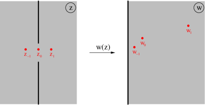
Figure 7: Conformal map from the quench geometry to the half-plane. Red dots indicate the locations of twist-field insertions and their images under $w(z)$.

The simplest choice for the subsystems is a bipartition ($B=\emptyset$) into two semi-infinite lines $A_{1}$ and $A_{2}$. One has then a single contact point and thus

$$\Tr(\rho_{A}^{T_{2}}(t))^{n_{e}}=\langle\mathcal{T}^{2}_{n_{e}}(z_{0})\rangle$$ (50)

where the expectation value of the twist fields has to be calculated on a world-sheet representing the time-evolved density operator $\rho(t)$. This is depicted on the left of Fig. 7, where the cut in the middle corresponds to the imaginary time evolution of two decoupled CFTs with fixed boundary conditions, yielding the initial state $\rho(0)$. The real time evolution takes place between the endpoints $z=\pm i\epsilon$ of the cut, and the twist field has to be inserted at $z_{0}=i\tau$. Note, that the parameter $\epsilon$ is needed to regularize the path-integral and the analytical continuation to real times $\tau=it$ must be carried out at the end of the calculation.

Although the original world-sheet has a complicated geometry, one can apply a conformal mapping [42]

$$w=\frac{z}{\epsilon}+\sqrt{\left(\frac{z}{\epsilon}\right)^{2}+1}$$ (51)

which transforms it to the half-plane, as shown on the right of Fig. 7. On the half-plane the expectation value of a one-point function is known and one can then use the conformal transformation formula to obtain

$$\langle\mathcal{T}^{2}_{n_{e}}(z_{0})\rangle\propto\left(\left|\frac{\mathrm{d}w}{\mathrm{d}z}\right|_{z_{0}}\frac{1}{\mathrm{Re}(w_{0})}\right)^{\Delta_{n_{e}}}$$ (52)

where $w_{0}=w(z_{0})$ and the scaling dimension of the operator $\mathcal{T}^{2}_{n_{e}}$ is given by [15]

$$\Delta_{n_{e}}=\frac{c}{6}\left(\frac{n_{e}}{2}-\frac{2}{n_{e}}\right)$$ (53)

with the central charge $c$. Carrying out the calculations, one obtains

$$\Tr(\rho_{A}^{T_{2}}(\tau))^{n_{e}}\propto\left(\frac{\epsilon}{\epsilon^{2}-\tau^{2}}\right)^{\Delta_{n_{e}}}$$ (54)

Continuing the result to real time $\tau\to it$, taking the limit $t\gg\epsilon$ and finally using Eq. (49), one arrives to the result in Eq. (34).

The local quench for the finite system can be treated in a similar way. There the world-sheet has a double-pants geometry, with fixed boundary conditions along $\mathrm{Re}(z)=\pm\ell$, and the proper conformal mapping to the half-plane was given in Ref. [43]. Carrying out the analogous steps, one arrives to the formula in Eq. (35).

On the other hand, the tripartite case in the infinite system with line segments $A_{1}=\left[-\ell,0\right]$ and $A_{2}=\left[0,\ell\right]$ is more involved. There, one has to consider the three-point function $\langle\mathcal{T}(z_{-1})\overline{\mathcal{T}}^{2}_{n_{e}}(z_{0})\mathcal{T}(z_{1})\rangle$ of the twist fields with $z_{0}=i\tau$ and $z_{\pm 1}=\pm\ell+i\tau$. This is mapped under (51) into a three-point function on the half-plane which, however, has the complexity of a six-point function on the full plane. Although some recent progress has been made in the derivation of higher order twist-field correlators in Ref. [48], their structure is rather involved and we have not been able to tackle this case analytically.

References

References

- [1] Amico L, Fazio R, Osterloh A and Vedral V 2008 Rev. Mod. Phys. 80 517
- [2] Calabrese P, Cardy J and Doyon B 2009 J. Phys. A 42 500301
- [3] Vidal G, Latorre J I, Rico E and Kitaev A 2003 Phys. Rev. Lett. 90 227902
- [4] Calabrese P and Cardy J 2009 J. Phys. A: Math. Theor. 42 504005
- [5] Eisert J, Cramer M and Plenio M B 2010 Rev. Mod. Phys. 82 277
- [6] Plenio M and Virmani S 2007 Quant. Inf. Comput. 7 1
- [7] Vidal G and Werner R F 2002 Phys. Rev. A 65 032314
- [8] Plenio M B 2005 Phys. Rev. Lett. 95 090503
- [9] Audenaert K, Eisert J, Plenio M B and Werner R F 2002 Phys. Rev. A 66 042327
- [10] Adesso G and Illuminati F 2007 J. Phys. A: Math. Theor. 40 7821
- [11] Marcovitch S, Retzker A, Plenio M B and Reznik B 2009 Phys. Rev. A 80 012325
- [12] Wichterich H, Molina-Vilaplana J and Bose S 2009 Phys. Rev. A 80 010304(R)
- [13] Wichterich H, Vidal J and Bose S 2010 Phys. Rev. A 81 032311
- [14] Calabrese P, Cardy J and Tonni E 2012 Phys. Rev. Lett. 109 130502
- [15] Calabrese P, Cardy J and Tonni E 2013 J. Stat. Mech. P02008
- [16] Calabrese P, Tagliacozzo L and Tonni E 2013 J. Stat. Mech. P05002
- [17] Alba V 2013 J. Stat. Mech. P05013
- [18] Chung C, Alba V, Bonnes L, Chen P and Läuchli A M 2014 Phys. Rev. B 90 064401
- [19] Lee Y A and Vidal G 2013 Phys. Rev. A 88 042318
- [20] Castelnovo C 2013 Phys. Rev. A 88 042319
- [21] Bernard D and Doyon B 2012 J. Phys. A: Math. Theor. 45 362001
- [22] Bernard D and Doyon B preprint arXiv:1302.3125
- [23] Eisler V and Zimborás Z 2014 Phys. Rev. A 89 032321
- [24] Ajisaka S, Barra F and Žunkovič B 2014 New J. Phys. 16 033028
- [25] Wolf M M, Verstraete F, Hastings M B and Cirac J I 2008 Phys. Rev. Lett. 100 070502
- [26] Spohn H and Lebowitz J L 1977 Commun. Math. Phys. 54 97
- [27] Boldrighini C, Pellegrinotti A and Triolo L 1983 J. Stat. Phys. 30 123
- [28] Ho T G and Araki H 2000 Proc. Steklov Inst. Math. 228 191
- [29] Ogata Y 2002 Phys. Rev. E 66 016135
- [30] Aschbacher W H and Pillet C A 2002 J. Stat. Phys. 112 1153
- [31] De Luca A, Viti J, Bernard D and Doyon B 2013 Phys. Rev. B 88 134301
- [32] Collura M and Karevski D 2014 Phys. Rev. B 89 214308
- [33] Collura M and Martelloni G 2014 J. Stat. Mech. P08006
- [34] Peres A 1996 Phys. Rev. Lett. 77 1413
- [35] Tóth G, Knapp C, Gühne O and Briegel H 2007 Phys. Rev. Lett. 99 250405
- [36] Anders J and Winter A 2008 Quantum Inf. Comput. 8 0245
- [37] Anders J 2008 Phys. Rev. A 77 062102
- [38] Ferraro A, Cavalcanti D, García-Saez A and Acín A 2008 Phys. Rev. Lett. 100 080502
- [39] Cavalcanti D, Ferraro A, García-Saez A and Acín A 2008 Phys. Rev. A 78 012335
- [40] Eisler V and Peschel I 2007 J. Stat. Mech. P06005
- [41] Eisler V, Karevski D, Platini T and Peschel I 2008 J. Stat. Mech. P01023
- [42] Calabrese P and Cardy J L 2007 J. Stat. Mech. P10004
- [43] Stéphan J M and Dubail J 2011 J. Stat. Mech. P08019
- [44] Stéphan J M and Dubail J 2013 J. Stat. Mech. P09002
- [45] Ares F, Esteve J, Falceto F and Sánchez-Burillo E 2014 J. Phys. A: Math. Theor. 47 245301
- [46] Karrasch C, Ilan R and Moore J E 2013 Phys. Rev. B 88 195129
- [47] Castro-Alvaredo O, Chen Y, Doyon B and Hoogeveen M 2014 J. Stat. Mech. P03011
- [48] Coser A, Tagliacozzo L and Tonni E 2014 J. Stat. Mech P01008