Spatial density fluctuations and selection effects in galaxy redshift surveys

Abstract

One of the main problems of observational cosmology is to determine the range in which a reliable measurement of galaxy correlations is possible. This corresponds to determine the shape of the correlation function, its possible evolution with redshift and the size and amplitude of large scale structures. Different selection effects, inevitably entering in any observation, introduce important constraints in the measurement of correlations. In the context of galaxy redshift surveys selection effects can be caused by observational techniques and strategies and by implicit assumptions used in the data analysis. Generally all these effects are taken into account by using pair-counting algorithms to measure two-point correlations. We review these methods stressing that they are based on the a-priori assumption that galaxy distribution is spatially homogeneous inside a given sample. We show that, when this assumption is not satisfied by the data, results of the correlation analysis are affected by finite size effects.In order to quantify these effects, we introduce a new method based on the computation of the gradient of galaxy counts along tiny cylinders. We show, by using artificial homogeneous and inhomogeneous point distributions, that this method is to identify redshift dependent selection effects and to disentangle them from the presence of large scale density fluctuations. We then apply this new method to several redshift catalogs and we find evidences that galaxy distribution, in those samples where selection effects are small enough, is characterized by power-law correlations with exponent $\gamma=0.9$ up to $20$ Mpc/h followed by a change of slope that, in the range [20,100] Mpc/h, corresponds to a power-law exponent $\gamma=0.25$. Whether a crossover to spatial unformity occurs at $\sim 100$ Mpc/h cannot be clarified by the present data.

1 Introduction

Galaxy redshift surveys represent one of the cornerstone of modern cosmology. In the past decades we have assisted to an exponential growth of the data [1, 2, 3, 4] which have revealed that galaxies are organised in a large scale network of filaments and voids. Statistical analysis of these surveys have shown that the galaxy distribution is characterised by power-law correlations in the range of scales [0.1-20] Mpc/h: whether or not on scales $r>80$ Mpc/h correlations decay and the distribution crossovers to uniformity, is still matter of considerable debate [5, 6, 7, 8, 9, 10, 11, 12, 13, 14, 15, 16, 17, 18, 19, 20, 21]. This debate was originated by the use of different statistical methods to measure two-point correlations, to estimate statistical and systematic errors and to control the selection effects that maybe present in the data (see, e.g., [5, 24]). Indeed, the construction of large enough galaxy redshift catalogues for a reliable statistical analysis represents a complex problem of observational astronomy. In general, observations are exposed to a variety of systematic effects that can non trivially affect the study of correlation properties. For instance, there are effects which depend on the observational strategy adopted to construct a particular sample, there are intrinsic physical effects which ultimately depend on the distance of a galaxy from us (e.g., galaxy evolutionary corrections, K-corrections, etc.), and corrections that must be applied to the data to built a three-dimensional sample suitable for a correlation analysis. In addition, several corrections require theoretical modelling and assumptions which can bring more uncertainty in the results of a data analysis. For these reasons it is important to assess the impact of selection effects on the statistical information derived from the study of the correlation function.

Standard methods based on pair-counting algorithms may correct for selection effects, but they are based on the a-priori assumption of spatial uniformity. In this paper, we introduce an analysis, called the gradient cylinder method (GCM), which is based on a small number of a-priori assumptions and that is suitable to identify selection effects in any kind of statistically isotropic and homogeneous distribution, bf i.e., even if the distribution is not uniform at large scales. This new method allows us to measure unambiguously the presence of redshift dependent selection effects in the data and to quantify their impact on the estimations of two-point correlations both for spatially homogeneous and inhomogeneous point distributions. We stress that the new method that we introduce here represents one of the test that can be applied to the data to detect radial dependent selection effects and it must be intended to be a complementary analysis that can provide with further elements to the characterisation of the statistical properties of a given sample. As we discuss below it is necessary that known luminosity selection effects are taken into account. However the usefulness of this new test lies in the fact that it can detect radial dependent selection effects that are generally not controllable with standard techniques.

The paper is organised as follows: firstly, in Sect.2, we discuss different methods and estimators of two-points correlations. Then we introduce the new method, based on the computation the gradient of galaxy counts in tiny cylinders. We show that this method is able to detect redshift-dependent selection effects in the data. In addition, we show that standard pair-counting estimators fail to detect the intrinsic correlation properties for intrinsically inhomogeneous distributions. Then, in Sect.3 we study and calibrate the method by using several distributions with a-priori known properties. Results in the different galaxy samples are then discussed in Sect.4. Finally in Sect.5 we draw our main conclusions.

2 Statistical methods

Two-point correlations can be characterised by determining the conditional density

$$\langle n(r_{12})\rangle dV_{1}dV_{2}=\frac{\langle n(\vec{r_{1}})n(\vec{r_{2}})\rangle}{n_{0}}dV_{1}dV_{2}\;,$$ (2.1)

where $n(\vec{r})$ is the microscopic number density and $n_{0}$ is the (ensemble) average density of the point distribution. Eq.2.1 gives the a-priori probability of finding two particles placed in the infinitesimal volumes $dV_{1},dV_{2}$ around $\vec{r_{1}}$ and $\vec{r_{2}}$ with the condition that the origin of the coordinates is occupied by a particle. A generic estimator of the conditional density can be written as

$$\left<n^{G}(r)\right>=\sum_{i=1}^{M}\frac{N_{i}(r)}{V_{i}(r)}\omega_{i}(r)=\sum_{i=1}^{M}n_{i}(r)\omega_{i}(r)\;,$$ (2.2)

where $M$ is the number of points in the sample, $N_{i}(r)$ is the number of points in the volume $V_{i}(r)$, $n_{i}(r)=N_{i}(r)/V_{i}(r)$ is the density, and $\omega_{i}(r)$ is a weight such that

$$\sum_{i=1}^{N}\omega_{i}(r)=1\;.$$ (2.3)

Different estimators correspond to different choices for the weights. When the volume is exactly the same for all points and it is fully included in the sample volume then $V_{i}(r)=V(r)\;$ and $\omega_{i}(r)=1\;\forall i$. This is the so-called full-shell (FS) estimator that can be simply written [5, 25, 26, 35] as

$$\left<{n(r)}\right>=\frac{1}{M(r)}\sum_{i=1}^{M(r)}\frac{N_{i}(r)}{V(r)}=\frac{1}{M(r)}\sum_{i=1}^{M(r)}n_{i}(r)\;,$$ (2.4)

where now, because of geometrical constraints, the number of points that contribute to the the average depends on the scale $r$, i.e. $M=M(r)$. It can be shown that this estimator is unbiased, i.e. its ensemble average in a finite volume is equal to the ensemble average. When instead the volume $V(r)$ may lie partially outside the sample then the estimator in Eq.2.2 is biased and the amplitude of the systematic bias is, as we discuss in more detail below, in general unknown [25, 26, 35].

Statistical errors affecting the determination of Eq.2.4 can be easily determined as

$$\sigma^{2}(r)=\frac{1}{M(r)}\sum_{i=1}^{M(r)}n_{i}^{2}(r)-\langle n(r)\rangle^{2}\;.$$ (2.5)

At scales comparable with the sample size the situation systematic errors become larger than statistical ones [9]. Indeed, on large scales the problem is that different determinations of the conditional density $n_{i}(r)$ are not independent anymore, as they explore the same volume because of the constraints imposed by the finiteness of the sample. For this reason it is not possible to properly estimate neither the conditional density, nor its variance at scales comparable with the sample size.

In the literature one may find other methods to estimate correlation function errors than that Eq.2.5. For instance several authors suggest that jack-knife methods actually recover the correct variance on large scales, but fail on smaller scales [33]. However, as it was discussed by the jack-knife is not a suitable method to estimate errors in the presence of long-range correlations for the lack of independence between different sub-samples [34]. Thus we will adopt the most conservative one given by Eq.2.5.

Note that the statistical errors computed through Eq.2.5 are in general negligible at all scales as long as the average is performed over a number of centres $M(r)>10^{2}$ (as we do it what follows). The main source of error in the measurement of the conditional density is thus represented by systematic errors, which are connected to finite-volume effects. In the past we have tested different methods to control and quantify such effects; we concluded that the most reliable one is represented by study, for each $r$, the full probability density function of the values of $n_{i}(r)$ entering in Eq.2.4 (we refer the interested reader to [9, 12, 13, 14] for a more detailed discussion of this issue).

The most natural and simpler choice for the volume $V(r)$ in the case of the FS estimator is a sphere. In this case the analysis is limited by the radius $R_{s}$ of the largest sphere that can be fully included in the sample volume. For typical surveys $R_{s}$ can be much smaller than the largest separation between the most distant pairs of galaxies $R_{max}\gg R_{s}$. A way to avoid this constraint is to employ the non-FS estimators of the correlation function used standardly in the cosmological literature [36, 37, 39, 38, 25]. Another possibility that we study in the next subsection is to implement the FS estimator in cylinders. We then review the problems of the non-FS estimators in Sect.2.2.

2.1 The full shell estimator in cylinders

In what follows, in Eq.2.4 we consider $V(r)$ to be the volume of a cylinder of height $2r$ and radius $h$ fully included in the sample volume. The point $i^{th}$ is now placed in the centre of the cylinder at distance $r$ from each of the two bases and in the centre of the circle of radius $h$. The cylinder volume is simply

$$V(r)=2r\times\pi h^{2}\;.$$

We take the generic cylinder to be oriented in a manner parallel to the line of sight (LOS) or perpendicularly to it. In the former case we determine the estimator $\left<{n^{p}(r;h)}\right>$, while in the latter case $\left<{n^{o}(r;h)}\right>$. If the distribution is isotropic we expect that

$$\left<n^{p}(r;h)\right>=\left<n^{o}(r;h)\right>=\left<{n(r)}\right>$$ (2.6)

where $\left<n(r)\right>$ is determined in spheres of radius $r$ (i.e., Eq.2.4).

The determination of whether the $i^{th}$ point can be included or not in the sum in Eq.2.4 requires the measurement of several distances necessary to control that the cylinder is fully included in the sample volume. In left panel of Fig.1 its shown the case where the cylinders are oriented along the LOS and in right panel the case in which the cylinders are oriented perpendicularly to the LOS: the points $P_{1},P_{2},P_{3},P_{4}$ determine the points where the straight lines from the origin of the coordinates $P_{0}$, intersect the boundaries of the sample (the generic galaxy is called $P$ and it is placed in the middle of a cylinder of height $2r$ and radius $h$, whose extremes are placed in the points $P_{A}$ and $P_{B}$).

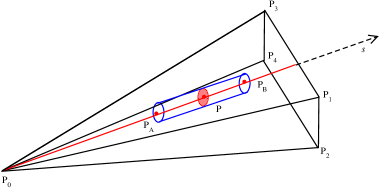
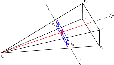
Figure 1: Left panel: geometry of the cylinder oriented along the line of sight. Right panel: geometry of the cylinder oriented orthogonally to the line of sight.

For cylinders oriented parallel to the LOS, the points $P_{A}$ and $P_{B}$ are placed on the line $s$ at distance $\pm r$ from the point $P$ while for cylinders oriented perpendicularly to the LOS the points $P_{A}$ and $P_{B}$ are placed on the line $t$ at distance $\pm r$ from the point $P$. Note that in the former case it is necessary to choose an orientation for the line $t$ orthogonal to $s$: for convenience, we choose parallel to the plane identified by the points $[P_{0},P_{2},P_{4}]$, but any other choice would be equally valid.

In summary, to verify that a generic cylinder is placed inside the boundaries of the sample, we have to control that the points $P_{A}$ and $P_{B}$ are indeed contained the sample volume and that their distance from the sample boundaries, orthogonally to the straight line $s$ or $t$, is smaller than $h$. Given these constraints, we compute for each cylinder, with the $i^{th}$ galaxy at its centre point, the number of points $N_{i}(r;h)$ contained in it; the density entering in the sum in Eq.2.4 , is then

$$n_{i}(r;h)=\frac{N_{i}(r;h)}{2\pi rh^{2}}\;.$$ (2.7)

In what follows $h$ is chosen to be slightly larger than the average distance between nearest neighbours: for smaller values of $h$ the number of points of contained in a generic cylinder of length $r$ is not sufficiently large to avoid a too high Poisson noise.

As mentioned above, in many cases the radius of the largest sphere contained in the sample volume $R_{s}$ is much smaller than the maximal distance between two galaxies $R_{max}\gg R_{s}$. In particular this situation occurs when the survey is very deep and covers a small solid angle in the sky [26]. Thus by measuring the conditional density in cylinders one can largely increase the range of measurements with a FS estimator: in principle it is possible to reach $R_{max}/2$ instead of $R_{s}$. However one must consider that this estimation involves the convolution of the correlation properties of a distribution with the cylinder window function. In order to understand the effect of the convolution of the cylinder window function with the shape of the two-point correlation function let us consider a few simple examples. We firstly suppose that in a sphere of radius $r$ the average conditional density has a simple power law behaviour:

$$\langle n(r)\rangle=\frac{A}{r^{\gamma}}$$ (2.8)

with $0\leq\gamma<3$. The density of points in the cylinder is

$$\langle n(r;h)\rangle=\frac{2}{2\pi rh^{2}}\int_{0}^{r}dx\int_{0}^{2\pi}d\phi\int_{0}^{h}\frac{A\rho d\rho}{(x^{2}+\rho^{2})^{\gamma/2}}\;.$$ (2.9)

For $\gamma=0$ (Poisson distribution) we simply find $\langle n(r)\rangle=A\;.$ When $\gamma>0$, by numerically integrating Eq.2.9, we find

$$\langle n(r;h)\rangle\approx\zeta(h)r^{3-\gamma}\;,$$ (2.10)

where the amplitude $\zeta(h)$ depends on $h$ (which is taken fixed) while the corrections to the leading $r^{3-\gamma}$ behaviour are negligible when $h\ll r$.

Let us now consider the case in which the conditional density in spheres has a change of slope:

$$\langle n(r)\rangle=\frac{A}{r^{\gamma_{1}}}\;\;\mbox{for}\;\;r\leq\lambda_{*}$$ (2.11)

$$\langle n(r)\rangle=\frac{B}{r^{\gamma_{2}}}\;\;\mbox{for}\;\;r\geq\lambda_{*}$$

with $0\leq\gamma_{2}\leq\gamma_{1}<3$ and where $B=A\lambda_{*}^{\gamma_{2}-\gamma_{1}}$ for continuity reasons. In addition, for simplicity we consider $h<\lambda_{*}$.

The results of the numerical integration for two particular cases (i.e., $\gamma_{1}=1$, $\lambda_{0}=20$ Mpc/h and $\gamma_{2}=0$ or $\gamma_{2}=0.25$) is shown in Fig.2: we can clearly conclude that, when the conditional density has a single power-law behaviour, by computing it in cylinders, one is able to measure the correlation exponent properly on scales larger than the cylinder radius $h$ thus extending the analysis to $R_{max}>R_{s}$. Instead, when the conditional density has a change of slope it is not possible, unless the samples extends over several decades, to reach a clear conclusion about the large scale exponent.

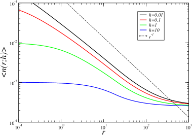
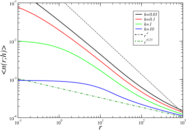
Figure 2: Behaviour of the conditional density given by Eq.2.11 estimated in cylindrical volumes of radius $h$. Left panel: $\gamma_{1}=1.0;\gamma_{2}=0.0\;$ and $\lambda_{0}=20$ Mpc/h. Right panel: $\gamma_{1}=1.0;\gamma_{2}=0.25\;$ and $\lambda_{0}=20$ Mpc/h.

2.2 Pair-counting estimators

Estimators of two-point correlations used standardly in the cosmological literature [36, 37, 39, 38, 25], are based on the determination of $\xi(r)$. This is related to the conditional density by the equation [26]

$$\langle n(r)\rangle={\bar{n}}\left(1+\xi(r)\right)$$ (2.12)

where ${\bar{n}}$ is the sample average density. It is well known that for inhomogeneous distributions the estimation of the sample density ${\bar{n}}$ depends explicitly on the sample size $R_{s}$ so is the estimation of $\xi(r)$ [26] . On the other hand, for distributions that are spatially uniform at scales smaller than the sample size $\langle n(r)\rangle$ is not affected by the sample finiteness and thus there is in principle no problem in the use of Eq.2.12, to jointly determine ${\bar{n}}$ and $\xi(r)$ for measuring $\langle n(r)\rangle$. The situation is however not so simple. As emphasised in [26] a great care must be taken in interpreting the results obtained from pair counting estimators from around the scale, of the order of $R_{s}$, at which partial shells begin playing an important role in these estimators, i.e. beyond the scale up to which one can calculate the FS estimator. The main problem is that the bias and variance of such estimators is calculable only in very simple cases (e.g., for the uncorrelated Poisson case), and it is uncontrolled (i.e. there is not an analytical control of their amplitude) for a broader class of distributions (see for more details [25, 40, 35]). That is, the bias and the variance of these estimators cannot be computed for a general point distribution and thus one can only constraint them through the use of a numerical simulations. Therefore only if assumes which are the large scale properties of a distribution one can measure reliable error bars through numerical simulations.

In what follows we will consider three popular (non full shell) estimators based on pair counting. The first one is the so-called Rivolo estimator [37] that gives equal weighting of all centres i.e. $\omega_{i}=\frac{1}{N}$ (see Eq.2.2) and thus gives equal weight to partial and full shells. For this reason it will have a variance which increases strongly at scales comparable to $R_{s}$. This can be written as

$$\frac{\left<n^{R}(r)\right>}{n_{0}}=\frac{N_{R}}{N_{D}(N_{D}-1)}\sum_{i}\frac{D_{i}(r)}{R_{i}(r)}$$ (2.13)

where ${N_{D}}$ (${N_{R}}$) is the number of data (random) points in the volume $V$, $n_{0}=N_{D}/V$ is the estimation of the sample density, and $D_{i}(r)$ ($R_{i}(r)$) is the number of data (random) points in the distance range $(r-\Delta/2,r+\Delta/2)$ from the point $i$. In what follows, we will consider the integrated value of this estimator, i.e. $D_{i}(r)$ and $R_{i}(r)$ calculated not in shells but in spheres, as this version of the Rivolo estimator was used by [19].

A very widely used estimator of $\xi(r)$ is the one introduced by Davis & Peebles (DP) [36]: the corresponding estimator of the conditional density is

$$\frac{\left<n^{DP}(r)\right>}{n_{0}}=\frac{2N_{R}}{N_{D}-1}\frac{DD(r)}{DR(r)}$$ (2.14)

where $DD(r)$ ($DR(r)$) is the number of data-data (data-random) pairs with separation in the range $(r-\Delta/2,r+\Delta/2)$. It is easy to verify that this corresponds a choice of weighting in Eq.2.2 (see [26])

$$\omega_{i}(r)=\frac{\Delta V_{i}(r)}{\sum_{i}\Delta V_{i}(r)}\;.$$

Partial shells are thus weighted in proportion to their volume. The idea for this choice is that this may compensate for certain distributions for the additional variance associated to the partial shells [25, 26].

The other estimator that we consider is related to the one introduced by Landy & Szalay (LS) [38]:

$$\frac{\left<n^{LS}(r)\right>}{n_{0}}=\frac{N_{R}(N_{R}-1)}{N_{D}(N_{D}-1)}\frac{DD(r)}{RR(r)}-2\frac{N_{R}-1}{N_{D}}\frac{DR(r)}{RR(r)}+2\;.$$ (2.15)

The LS estimator is the most popular in the cosmological literature because it has the minimal variance for a Poisson distribution of points, with a variance which is proportional to $1/N$ rather than $1/\sqrt{N}$ for the other estimators considered. This estimator was found to have the minimal variance also in the case of a distribution extracted from a standard LCDM simulation. [40]. Note that the theoretical errors in the correlation function can be estimated analytically for any uniform distribution once it is given the power spectrum [41]: the difficult problem lies in the estimation of the errors in the regime of strong clustering.

2.3 The gradient of galaxy counts in cylinders

In addition to the estimation of the conditional density in cylinders we can compute the galaxy counts gradient in cylinders oriented along the LOS: we show below its usefulness. This can be estimated by

$$\delta^{p}(r;h)=\frac{\langle N_{N}(r;h)\rangle-\langle N_{F}(r;h)\rangle}{\langle N(r;h)\rangle}\;,$$ (2.16)

where we have defined

$$\langle N(r;h)\rangle=\frac{1}{M(r)}\sum_{i=1}^{M(r)}N_{i}(r;h)\;,$$ (2.17)

while $\langle N_{N}(r;h)\rangle$ ($\langle N_{F}(r;h)\rangle$) is defined similarly to Eq.2.17 but it is computed in a cylinder of length $r$ (instead of $2r$) and radius $h$. In particular, for $\langle N_{N}(r;h)\rangle$ ($\langle N_{F}(r;h)\rangle$) the $i^{th}$ centre-point is located at the base which has the largest (smallest) radial distance (see the upper panel of Fig.1).

Similarly to Eq.2.16 we define the analogous quantity for cylinders oriented orthogonally (see the bottom panel of Fig.1):

$$\delta^{o}(r;h)=\frac{\langle N_{L}(r;h)\rangle-\langle N_{R}(r;h)\rangle}{\langle N(r;h)\rangle}$$ (2.18)

where $\langle N_{L}(r;h)\rangle$ is the average number of points contained in the half cylinder delimited by $[P,P_{A}]$ and $\langle N_{R}(r;h)\rangle$ in the other half cylinder delimited by $[P,P_{B}]$.

In what follows we will show that the joint determination of $\delta^{p}(r;h)$ and $\delta^{o}(r;h)$ in a galaxy catalogues, may shed light on the presence of intrinsic fluctuations and extrinsic radial dependent selection effects. We will refer to these determinations as the gradient cylinder method (GCM).

Note that, in general, that $\delta^{p}(r)$ ($\delta^{o}(r)$) is non-zero when there is a systematic difference between $\langle N_{N}(r;h)\rangle$ and $\langle N_{F}(r;h)$ (or between $\langle N_{L}(r;h)\rangle$ and $\langle N_{R}(r;h)$) which is persistent in space. On the one hand, when this is due to a selection effect in the direction parallel (orthogonal) to the line of sight $\delta^{p}(r)$ ($\delta^{o}(r)$) will show a well defined trend, i.e. a systematic increase or decrease of its amplitude with the scale $r$. On the other hand, when this is due to large scale structures $\delta^{p}(r)$ ($\delta^{o}(r)$) will be characterised by fluctuations so that its amplitude will be different from zero for a range of scales correspondent to the spatial extension of the structures.

3 Tests of selection effects on artificial distribution

In order to illustrate the usefulness of the GCM introduced in Sect.2.3, we apply it to point distributions with known properties that can be, or not, affected by a radial selection $f(s)$, again with controlled properties. The exercises that are discussed in what follows show that the intrinsic correlation properties can be distorted by a radial selection function $f(s)$ (where $s$ is the radial distance from the Earth) and that the study of the quantities $\delta^{p}(r;h)$ and $\delta^{o}(r;h)$ (Eqs.2.16-2.18) can reveal the presence of a radial selection. We show that the application of the GCM works equally well for uniform and inhomogeneous distributions. On the other hand, to emphasise the limits of standard pair-counting estimators, we also consider some example of the determination of the conditional density with pair-counting methods. These will be useful to show that both the bias and the variance of these estimators, determine their large scale behaviour.

We note that the artificial samples that we considered to test our method are already volume limited. We assume that the observational selection effect related to the limit in apparent magnitude imposed by the observations, as it is a well known problem, has been already taken into account in the construction of a proper sample for statistical analysis.

The artificial galaxy distributions, each with $N=10^{5}$ points, have been generated, in a box of side $L=1000$ Mpc/h, by using three different algorithms: (1) a purely Poisson process (2) a random walk and a (3) a random trema dust [26]. We have then chosen a random point close to the edge of the cube to be the origin of coordinates of a spherical volume limited by ascension right $\in[0,\pi/2]$, declination $\in[0,\pi/2]$ and radial distance from the origin $s\in[0,500]$ Mpc/h. We have then applied to the artificial galaxy a radial dependent selection of points described by the following function of the (radial) distance from the origin of coordinates:

$$f(s;\alpha)\sim s^{-\alpha}\;.$$ (3.1)

The amplitude of the selection function is tuned to eliminate a relevant fraction (i.e., $>20\%$) of the original distribution points.

The radial density clearly becomes

$$n(s;\alpha)=n(s)\times f(s;\alpha)\;.$$ (3.2)

In addition, a mock galaxy distribution was constructed from a cosmological LCDM N-body simulation in a box of side $l=500$ Mpc/h[27]. Even in this case we have then randomly chosen a mock galaxy close to one of the edges of the simulation box to be the origin of coordinates. We have then cut a spherical volume limited as for the artificial distributions discussed above. Then we have applied to these data a selection function again described by Eq.3.2.

3.1 Poisson

We first consider a Poisson distribution: given the absence of spatial correlations we find

$$n(s)|_{s=r}\approx\left<{n(r)}\right>\approx\left<{n^{p}(r;h)}\right>\approx\left<{n^{o}(r;h)}\right>\approx const.\;,$$ (3.3)

where $n(s)$ are the galaxy counts per unit volume as a function of the radial distance $s$ from us and where the equality in Eq.3.3, valid for $r=s$, is due to the fact that the point distribution has no correlations. In addition we find $\delta^{p}(r;h)\approx\delta^{o}(r;h)\approx 0$, in agreement with the expectation for an isotropic distribution of points.

We have then applied to the data a selection function of the type described by Eq.3.2 In Fig.3 we report the results obtained by changing $\alpha~{}\in~{}[-1,2]$: in this case we simply find $n(s;\alpha)\sim s^{\alpha}$ .

In order to measure the departure of the conditional density for $\alpha\neq 0$, i.e. $\left<{n(r)}\right>_{\alpha\neq 0}$ from its unperturbed shape $\left<{n(r)}\right>_{\alpha=0}$ we may the quantity

$$\kappa(r)=\left|\frac{\left<{n(r)}\right>_{\alpha\neq 0}-\left<{n(r)}\right>_{\alpha=0}}{\left<{n(r)}\right>_{\alpha=0}}\right|$$ (3.4)

which measures the percentage change in $\langle n(r)\rangle$ when a radial selection effect is imposed to the underlying distribution. We note that a $\delta^{p}(r)=0.1$ is indicative approximately of a 10% change in $\langle n(r)\rangle$. The conditional density has a percentage change in its amplitude only when the exponent of the radial selection function is $\alpha\geq 1$: correspondingly $\delta^{p}(r;h)$ grows with $r$ as $\langle N_{N}(r;h)\rangle>\langle N_{F}(r;h)\rangle$ (see Eq.2.16). Note we find $\delta^{o}(r;h)\approx 0$ as there is not any redshift dependent selection effect in the direction orthogonal to the LOS.

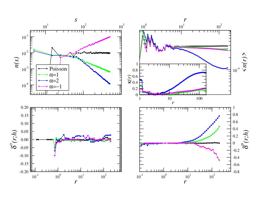
Figure 3: The case of a Poisson distribution to which it was applied a radial selection function described by Eq.3.1: the value of the exponent $\alpha$ is reported in the labels. Upper left panel: radial density $n(s)$. Upper right panel: conditional density $\left<{n(r)^{s}}\right>$ (in the inset panel it is reported the behaviour of $\kappa(r)$ — see Eq.3.4). Bottom left panel $\delta^{o}(r;h=1)$ (Eq.2.18). Bottom right panel: $\delta^{p}(r;h=1)$ (Eq.2.16)

3.2 Strongly correlated distributions

We have repeated the same tests on strongly correlated distributions: (i) a fractal with dimension $D=2$ generated by a random walk and (ii) a fractal with $D=2.7$ generated by a trema dust algorithm [26] . As for the Poisson distribution we have applied to the data a radial selection of the type described by Eq.3.1 with different $\alpha$ (see results in Fig.4 and Fig.5). The main results are in line with the behaviours discussed for the Poisson case:

• for $\alpha=2$ the conditional density sensibly changes its shape corresponding to $\kappa(r)>0.1$. For $\alpha=1$ the power-law behaviour of $\left<{n(r)}\right>$ is weakly affected by selection effects: the best fit exponent changes from $\gamma=-1.1$ to $\gamma=-1.3$. Instead, for $\alpha<0$ the difference with the unperturbed conditional density is manifested at large scales only.

• $\delta^{p}(r;h)$ is a very efficient diagnostic to detect radial dependent effects as it shows a clear systematic behaviour as a function of scale $r$ for different values of $\alpha$. In particular when $\delta^{p}(r;h)>0.1$ we observe a notable difference in the behaviour of the conditional density in spheres, i.e. $\kappa(r)>0.1$.

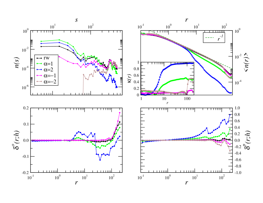
Figure 4: As Fig.3 but for case of strongly correlated distribution, corresponding to a fractal with $D=2$.

It is interesting to note that $\delta^{o}(r;h)$ is now much more fluctuating than it was for the Poisson case. These fluctuations, which however are limited in amplitude, are caused by both spatial structures when $\alpha$ is small and selection effects when $\alpha$ is large enough. Indeed, we recall that when the cylinders are oriented orthogonally to the line of sigh passing for their centres, at large $r$, they get contributions from points with an increasing radial distance.

The radial density can be very easily changed by a selection function of the type given in Eq.3.1. The use of the GCM, i.e. the analysis of $\delta^{p}(r;h)$ and $\delta^{o}(r;h)$, is able to reveal the presence of a radial selection that is shown by a systematic trend in $\delta^{p}(r;h)$.

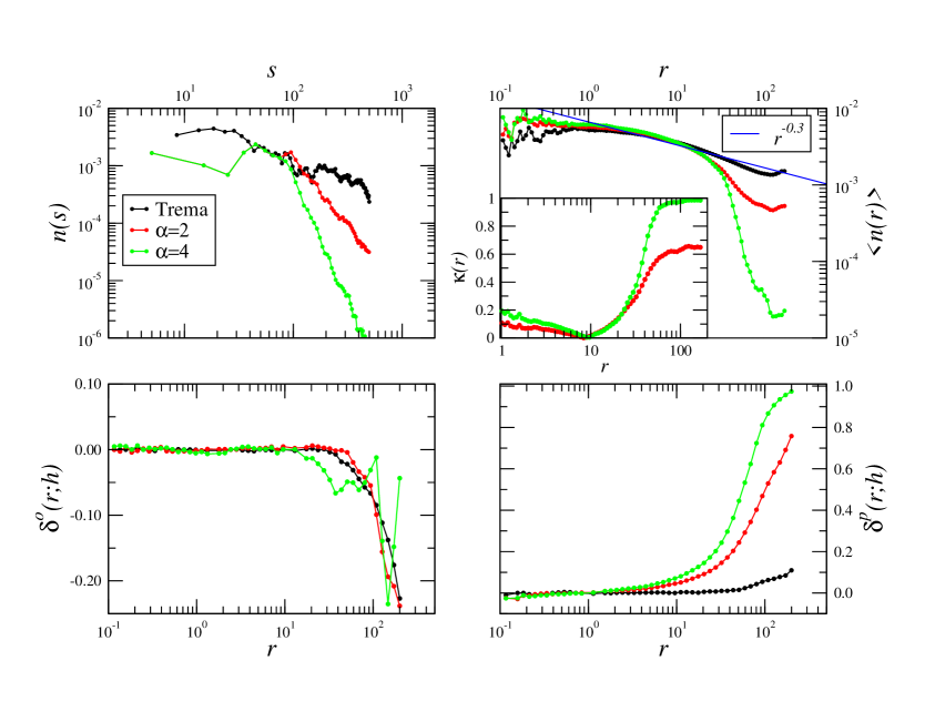
Figure 5: As Fig.3 but for case of strongly correlated distribution, corresponding to a fractal with $D=2.7$.

3.3 Mock galaxy catalogues

A mock galaxy distribution, constructed by a cosmological LCDM N-body simulation [27], represents an intermediate situation between a strongly clustered and a uniform distribution. Indeed, the conditional density (see Fig.6) shows a power-law behaviour at small scales, i.e. $r<20$ Mpc, while it flattens at large ones. Correspondingly, at large enough distances, the radial density presents fluctuations that are larger than a purely Poisson case, but symmetric (on average) around a constant behaviour. As for the other cases previously considered, we note that the behaviour of $\delta^{p}(r;h)$ is again a very good diagnostic of the presence of radial selection effects: for $\alpha>0$ we have that $\delta^{p}(r;h)$ grows with the scale $r$ and for $\alpha<0$ we find that $\delta^{p}(r;h)$ decreases.

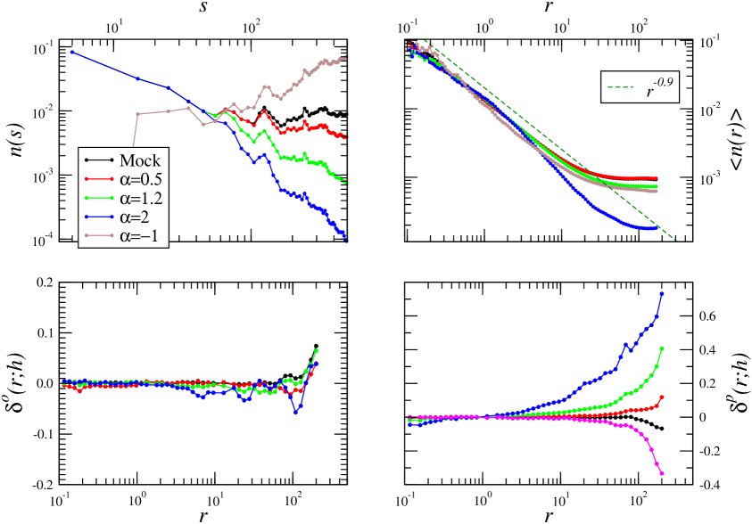
Figure 6: As Fig.3 but for the case of a mock galaxy catalogues.

3.4 Tests on pair counting estimators

We have used the four estimators introduced above: (i) the FS (Eq.2.4), (ii) the integrated Rivolo (Eq.2.13), (iii) the DP (Eq.2.14) and (iv) the LS (Eq.2.15) estimator to compute the conditional density both in the case of the random walk and of the trema dust. Note that for the three estimators based on pair counting we used 10 times random points than in the original data sample. Galaxies and mock random samples have the same radial selection function.

At small enough scales, i.e. $r\ll R_{s}\sim 150$ Mpc all estimators give similar results: in particular, the slopes are similar. The large finite size fluctuations that characterise a fractal distribution affect differently each estimator and thus the amplitude (once normalised to the sample average) is not the same in the different cases. On scales $r\approx R_{s}$ or larger, i.e. the limit of the FS estimator, we find that the three pair-counting estimators show a clear flattening although the behaviour for $r>R_{s}$ is different for the two fractals with $D=2$ and $D=2.7$ (see Fig.7). Therefore the large scale behaviour, i.e. $r\sim R_{s}$ and larger, of the conditional density is clearly completely spurious. Even the FS estimator shows changes in its behaviour on scales comparable to $R_{s}$, where by construction there should be no changes in the underlying correlation properties: these are due to finite volume effects. For comparison, we also show the FS estimator in a sample of double side $R^{*}_{s}=2R_{S}=300$: while the tail for $r\approx R^{*}_{s}$ is affected by finite size effects, at scales of the order of $R_{s}$ the FS estimator presents the expected behaviour.

We note that other estimators of the correlation function than the FS one, based on pair-counting, are affected by systematic effects that are not analytically calculable. In particular, the different small amplitude is due to a different way of calculating the sample density: even the simplest estimator of the sample density

$$n_{S}=\frac{N}{V}\;,$$

where $N$ is the number of galaxies contained in the sample volume $V$ is not an unbiased estimator, i.e. it does not satisfy to the condition that

$$\langle n_{S}\rangle=n_{0}$$ (3.5)

where $\langle...\rangle$ is the ensemble average in the finite volume and $n_{0}$ is the ensemble average [26]. The bias in this measurement of the sample density depends thus on how the estimator is constructed and it enters as an overall normalising factor. This thus is manifested even at small spatial scales. In addition, other systematic effects, which are different for different estimators, are manifested on scales of order of, or larger than, the radius of the maximum sphere that can be fully enclosed in the sample volume. In general, the smaller the fluctuations, and thus the larger is the fractal dimension, the smaller are the differences between the different estimators.

The precise break down of the power law and the shape of the transition to “uniformity” depends on the convolution of the intrinsic correlation properties of the distribution with the window function of the sample. In addition, different estimators show different large scale behaviours: the variance of each estimator cannot be controlled for arbitrary distributions and this is the reason why we use a conservative approach using the FS estimators (see also discussion in [26]).

We have performed other tests by considering mock LCDM galaxy samples (see below), with or without a radial selection, instead of a highly inhomogeneous one. We found that only in the case of LCDM point distribution with a smooth radial selection of the type described by Eq.3.1 one is able, by using a pair counting algorithm and a random Poisson distribution with the same radial distance counts $n(s)$ of the data, to “correct” for the effect of the selection function.

On the other hand, when the distribution is inhomogeneous any measurement of the conditional density (or of $\xi(r)$) with estimators that are not the FS gives a spurious results for $r>R_{s}$. For this reason we conclude that estimations of the conditional density like those determined by [19], cannot demonstrate that galaxy distribution is uniform but, at best, can reconstruct galaxy correlations if the distribution is uniform at scales much smaller than those of the sample. This is the standard procedure adopted in three-dimensional clustering analyses, and it is based on the assumption that galaxy distribution is spatially uniform inside the given sample and that the cosmology close to LCDM. Indeed, as shown in Fig.8, the different estimators of the conditional average density agree when they are computed in a sample with small large scales fluctuations, as it it the case of a realisation of a LCDM universe. However, as our aim is indeed to determine whether this is the case or not, we will not use an other estimator than the FS one.

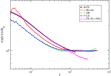
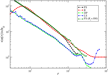
Figure 7: Conditional average density computed for the trema dust with $D=2.7$ (left panel) and a random walk with $D=2$ (right panel) with different estimators: Full-Shell in spheres, Rivolo, Davis and Peebles, Landy and Szalay. Note that the estimator of the conditional density has been normalised to the value of the of the sample density $n_{0}=N/V$ (where $N$ is the total number of objects in the sample of volume $V$).

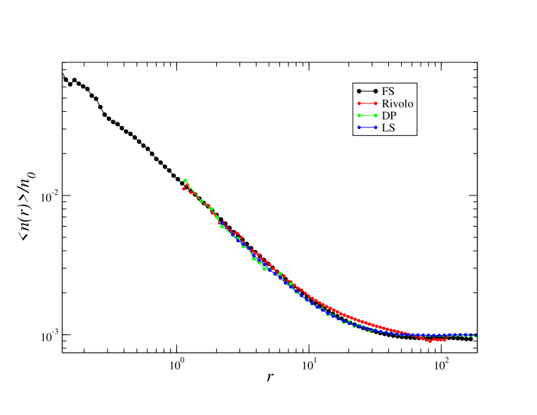
Figure 8: Conditional average density computed with different estimators in the mock LCDM.

3.5 Discussion

To summarise we have found that the conditional density is very weakly dependent on moderate selection effects in the data both for spatially uniform and non-uniform point distributions. Indeed only for a radial selection of the type $f(s)\sim s^{-\alpha}$ with $|\alpha|\geq 2$ the conditional density sensibly changes it shape. In addition, we have shown that the GCM is a very efficient tool to reveal radial selection effects in data working equally well for a uniform distribution and for an inhomogeneous one. In particular the results is Sect.3 allow us to conclude that the measurement of the conditional density varies less than 10%, i.e. $\kappa(r)<0.1$ (see Eq.3.4) when the gradient of the galaxy counts along the line of of sight (see Eq. 2.16) is $\delta^{p}<0.1$. We stress that our method suggests that if a sample has $|\delta^{p}(r)|<0.1$, and if the sample satisfy all other standard tests, like the obvious one of constructing a volume limited sample instead of considering a magnitude limited one, then the results can be trusted.

Then, we have pointed out that, in order to make a reliable estimation of large two-point correlations one needs to use the FS estimator of the conditional density. The main uncertainty of this estimator is represented by systematic errors which are important at the scale of the sample and of which we are not able to give a quantitative estimation but only identify their presence through the study e.g., of the probability distribution of spatial fluctuations [9].

We note that the relation between the behaviours of $\delta^{p}(r;h)$ and $n(s)$ is not uniquely determined. This is shown by the simple case of a Poisson distribution with a radial selection of the type $f(s)\sim s^{-1}$ and and a fractal with dimension $D=2$. In both cases we find the radial density decays as $n(s)\sim s^{-1}$, but only in the former case $\delta^{p}(r;h)\approx const.$. Thus, in general, it is not possible to predict the behaviour of the radial distance, or of the conditional density, from the knowledge of $\delta^{p}(r;h)$.

4 Results on real galaxy samples

The samples for which we present the analysis in this section are briefly discussed in Sect.A.

4.1 Sloan Digital Sky Survey

We have considered three different sample of the Sloan Digital Sky Survey (SDSS) [1]: the Main Galaxy (MG) sample [28, 29], the Luminous Red Galaxy (LRG) sample [30, 31] and the Quasar (QSO) sample [32].

4.1.1 Sloan Digital Sky Survey Main Galaxy Sample

We begin by discussing the behaviour of the FS estimator of the conditional density, i.e. Eq.2.4, in the six VL samples of the Sloan Digital Sky Survey (SDSS) (see Sect.A.1.1 and Tab.1). In order to evaluate the value of the cylinder radius, we have computed the nearest neighbours (NN) distribution and their average distance $\Lambda$. We found that $\Lambda\approx 1-4$ Mpc/h for the various samples. Note that for MG VL samples we have tested the FS estimators of $\langle n(r)\rangle$ in cylinders converge to a stable estimation for $h\geq 1$ Mpc/h, while for the LRG samples (see below) this convergence occurs $h\geq 10$ Mpc/h.

The behaviour of the conditional density is reported in Fig.9. One may note that in all samples we find a consistent result for the FS estimator in spheres. In particular we measure a power law behaviour $\sim r^{-\gamma}$ with $\gamma=0.9\pm 0.05$ in the range $[1,20]$ Mpc/h: the value of the slope and it error refer to the average over the six VL samples considered. At larger scales we find $\gamma=0.25\pm 0.05$ in the range $[20,110]$ Mpc/h .

Note that in this case the fits extends for less than a decade and thus one can easily find other possible fits with a functional form of the conditional density different from a simple power-law. However we conclude that at $\sim$ 100 Mpc/h a clear crossover toward homogeneity has not been yet reached. As discussed in [13] the nontrivial scaling behaviour of the average conditional density (and of its variance) correspond to fluctuations obeying the Gumbel distribution of extreme value statistics: we refer to [9, 13, 14] for a more extensive and detailed discussion of the variance and of the whole probability distribution of fluctuations.

The conditional density in cylinders $\left<n^{p}(r;h)\right>$ and $\left<n^{o}(r;h)\right>$ show, for $r<10$ Mpc/h, show a different slope that can be interpreted as due to the effect of peculiar velocities. Indeed, because of the effect of peculiar velocities, structures, at small scales are more elongated along the line of sight than in any other direction. Thus in the range of scales where the deformation of peculiar velocities $v_{p}$ is relevant, i.e. such that $r\approx v_{P}/H_{0}\leq 10$ Mpc/h, the conditional density along the line of sight is almost constant. Instead, on larger scales $\left<n^{p}(r;h)\right>$ approaches, with a different amplitude, the same scale dependent behaviour as $\left<n^{o}(r;h)\right>$.

Moreover, the conditional density in parallel cylinders, of $\left<n^{o}(r;h)\right>$, shows a change of slope at scales of the order of $\sim 100$ Mpc/h for $h=1$ Mpc/h. Whether this corresponds to a crossover toward homogeneity or a change of slope cannot be sorted out by this analysis. Indeed, as discussed in Sect.2.1, when the conditional density in spheres is characterised by a change of slope (as the one described by Eq.2.11) the large scale behaviour of $\left<n^{o}(r;h)\right>$ or of $\left<n^{p}(r;h)\right>$ does not clearly determine the correlation exponent as shown by the example in Fig.2.

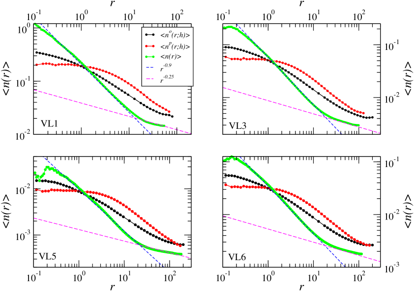
Figure 9: Behaviour of the conditional density computed in spheres and in cylinders of radius $h=1$ Mpc/h in several VL samples of the SDSS survey.

The behaviour of the radial density and of $\delta^{o}(r;h)$ and $\delta^{p}(r;h)$ is reported in Fig.10. One may note that $\delta^{o}(r;h)\leq 0.1$ but for the VL2 where, due to a large scale fluctuation, it slightly increases its value. On the other hand $\delta^{p}(r;h)\approx 0.1$ only for the VL4 and VL5: the decrease of $\delta^{p}(r;h)$ for $r>100$ Mpc/h corresponds to the fact that the radial density $n(s)$ increases for large radii. However this increase does not seem sufficient to change the behaviour of $\langle n(r)\rangle$ at large scales, whose behaviour is compatible with that found in other samples.

The increase of $\delta^{p}(r;h)$ for $r>100$ Mpc/h corresponds to the large differences found by [9, 44] in the probability distribution of fluctuations at large scales, i.e. $r>100$ Mpc/h, in these same samples. Whether or not a radial dependent selection effect, as the significant evolution hypothesised by [45], contributes to the behaviour of $\langle n(r)\rangle$ and $\delta^{p}(r;h)$ for $r>100$ Mpc/h in these samples cannot be definitively clarified from these data.

Note that the effect of peculiar velocities on small scales, that is shown by the difference in the behaviour between $\left<n^{o}(r;h)\right>$ and $\left<n^{p}(r;h)\right>$ on scales of order ten Mpc, is not detectable in the analysis of $\delta^{p}(r;h)$ as on small scales there are few points in the cylinders. One could increase the cylinder radius $h$ but then taking $h=10$ Mpc/h one looses the small scale effects as well.

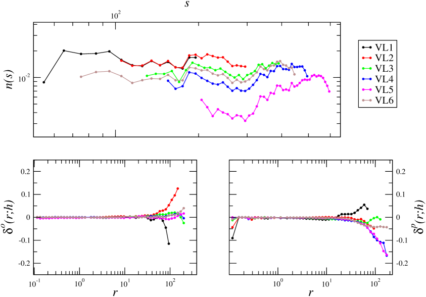
Figure 10: As for Fig.11 but for the six VL samples of the SDSS survey: note that both the radial density $n(s)$ and the conditional density in spheres have been normalised by an arbitrary factor.

In order to show the effect of a large scale radial selection we have studied the SDSS ML sample. In particular we have considered a sub-sample limited by $r\in[100,400]$ Mpc/h and a sub-sample limited by $r\in[100,1000]$ Mpc/h. Results are shown in Fig.11. One may note that in the deeper sub-sample $n(s)$ presents a sharp decay related to the fact that at large enough distances only very bright galaxies are included in the sample. Correspondingly the conditional density in spheres decays faster than for the VL samples but this is spurious behaviour as shown by growth of $\delta^{p}(r;h)$ at large scales. Instead, in the former sub-sample $n(s)$ gently decay but $\delta^{p}(r;h)$ again shows the effect of the biased luminosity selection. Note that, in this case, $\langle n(r)\rangle$ flattens at $r>100$ Mpc/h: this is a spurious effect due to the (known) radial selection affecting the ML sample. At least, in the VL samples that are not affected by the stronger luminosity selection effect, we do not detect such a clear flattening.

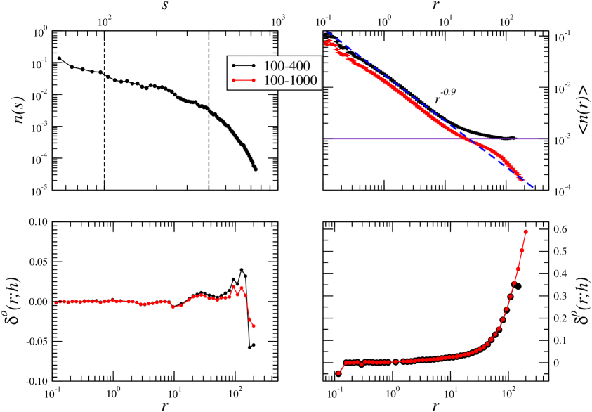
Figure 11: The case of the SDSS-ML sample. Upper left panel: radial density $n(s)$. Upper right panel: conditional density $\left<{n(r)^{s}}\right>$. Bottom left panel $\delta^{o}(r;h=1)$ (Eq.2.18). Bottom right panel: $\delta^{p}(r;h=1)$ (Eq.2.16).

4.1.2 Sloan Digital Sky Survey Luminous Red Galaxies Sample

In Fig.12 we show results for the LRG samples. In particular, we considered the Dim and Full samples and, for comparison, the Full sample limited by radial distances in the range $[10^{3},1.5\times 10^{3}]$ Mpc/h — we call this sample Full-LS (see Sect.A.1.2). This latter was chosen to see clearly the effect of the large scale selection effect present in these data. One may note the radial density decays as $\sim r^{-1}$ up to $\approx 800$ Mpc/h, lowering its amplitude by a factor $\approx 3$, then it grows by a factor $2$ in the range $800-1000$ Mpc/h and finally for $r>1000$ Mpc/h it decays sharply. As mentioned above this latter decay is due a known luminosity selection effect. The question is whether the other large scale trends are due to other selection effects, and thus to the fact that the sample is quasi VL, or to intrinsic fluctuations.

The conditional density in spheres for the LRG samples approaches an almost constant value for $r>80$ Mpc/h. However $\delta_{p}$ systematically increases at scales larger than $\sim 50\div 100$ Mpc/h with an amplitude that depends on the different magnitude/redshift cut used. Clearly in the LRG-Full-LS we observe the more clear trend with the largest value of $\delta_{p}\approx 0.1$ at 100 Mpc/h. This is certainly related to the sharp break of $n(r)$ beyond 1000 Mpc/h. On the other hand the LRG-Dim sample shows $\delta_{p}\approx 0.1$ only at $\approx 100Mpc/h$ and the same occurs to the LRG-Full which is the sum of the previous two samples. While the growth for LRG-Full for scales $r>100$ Mpc/h is again related to the sharp break of the radial density for $r>1000$ Mpc/h, present also in this sample, it is unclear why the LRG-Dim sample shows a systematic increase in the range [100,200] Mpc/h as in this case there are not known selection effects at work. Therefore given that we are unable to draw a clear identification of selection effects in this sample and because beyond $\sim 10$ Mpc/h the behaviour of $\langle n(r)\rangle$ is different in the LRG samples and in the sample MG-VL6 our conclusion is that we need a larger sample to confirm the the transition of homogeneity at $80$ Mpc/h that was claimed to be identified by [6]. It is worth to stress that our measurements, but not our interpretation for the reasons discussed above, agree with the results of [6].

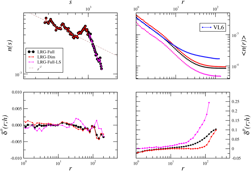
Figure 12: As for Fig.11 but for the three LRG samples of the SDSS survey (the cylinder radius is $h=10$ Mpc/h). For comparison we reported the FS estimator of the conditional density in sphere for VL6-SDSS (see Fig.9).

4.1.3 Sloan Digital Sky Survey Quasar Sample

The behaviours of the various statistics for the QSO SDSS samples (see Sect.A.1.3 for more details) are shown in Fig.13. One may note that the VL sample is characterised by a major radial selection effect which dominates the estimation of correlation properties. On the other hand, in the ML sample used by [20, 21] the radial density is approximately constant: this behaviour cannot be, however, interpreted as an evidence in favour of spatial homogeneity for the following reasons.

For a static population of uniformly distributed objects one expects to find: (i) a constant density in a VL sample and (ii) a density distributing $n(z)$ which reflects the selection function of the survey, i.e., that decays on large enough scales as for the magnitude limited sub-sample of the MG sample discussed above. In the VL-QSO sample we find instead that $n(z)$ increases at higher redshifts while it is almost constant in the QSO-ML sample. These peculiar behaviours occur because there must a strong selection effect intervening in these samples. This is related to the fact that properties of quasars are known to evolve with time because of the rate of mergers etc., and the redshift interval is very large, corresponding to more than 2 Gyr difference in look-back time. For this reason neither the VL nor the ML sample provide a sample of similar objects.

The QSO ML sample has thus a nearly constant density as a function of redshift: this is a coincidence probably due to QSO evolution. We thus conclude that this QSO sample is still not suitable for measuring QSO correlation properties in three dimensions. On the other hand studies (see, e.g., [22, 23]) using QSO samples for the derivation of correlation properties must necessarily adopt a number of ad-hoc assumptions to treat the redshift-dependent trends that characterise these samples. Here we have shown that these assumptions play a central role for deriving any result.

Note that the GCM we have introduced is tuned to detect simple radial dependent selection effects. However for the QSO samples the GCM alone is not able to clarify the situation as this is more complex than for a low redshift galaxy samples. Indeed, in this case, in addition to a luminosity selection effect which is by construction present in the magnitude limited sample, the QSO are affected by a redshift dependent physical effect, most probably evolution. Thus in order to understand what is going on in these data, one has to combine the GCM with the analysis of the radial density in magnitude and volume limited samples. The results of this analysis is that, although $|\delta^{p}(r)|<0.1$, these sample are affected by large redshift dependent selection effects, that are both observational (e.g., the magnitude limited selection) and physical (QSO evolution).

The case of the QSO-ML sample shows indeed that our new criteria is complementary to the standard way to define a proper sample for statistical analysis. Indeed in addition to have $|\delta^{p}(r)|<0.1$, one should always include the well-known and obvious procedure of avoiding to use a magnitude limited sample.

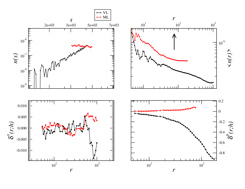
Figure 13: As for Fig.11 but for the VL and the ML SDSS quasars samples. In this case and with $h=75$ Mpc/h. The arrow indicates the average distance between nearest neighbours.

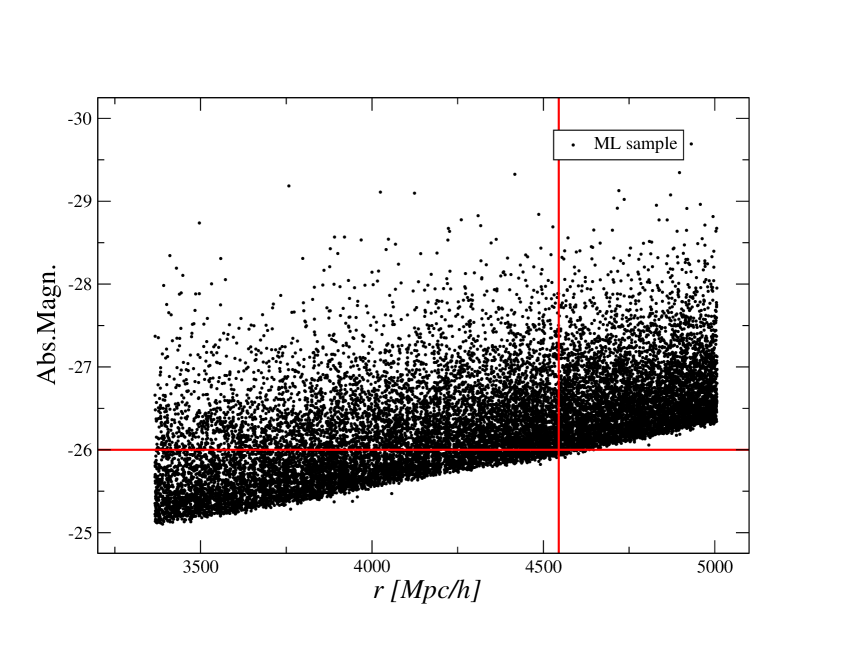
Figure 14: Distance-absolute magnitude diagram for the Sloan Digital Sky Survey Quasar Sample. One may note that the full magnitude limited sample is affected by a major selection effect that introduces a bias in the luminosity of objects as a function of their distance. That is, intrinsically bright object are visible at all scales while intrinsically fain object are included in the survey only if their distance is small enough. Such a situation makes unsuitable the magnitude limited sample for a correlation analysis. In the diagram a VL sample covers a rectangular area.

4.2 The Two Degree Field Galaxy Redshift Survey

In this and in the following section we have consider two galaxy redshift surveys which cover a smaller volume than SDSS but they allow an independent determination of the conditional density, although at a smaller scale than SDSS, in different sky regions and for different galaxies, as the selection properties of these surveys are very different from SDSS.

Results for the Two Degree Field Galaxy Redshift Survey (2dFGRS) VL samples (see Sect.A.2) are shown in Fig.15. One may note that the radial counts $n(s)$ show a sequence of fluctuations, that correspond to large scale structures and voids. Indeed, $\delta^{p}(r;h)$ does not present any large scales trend, while $\delta^{o}(r;h)$ fluctuates at very large scales because of the intrinsic fluctuations (structures) present in the sample NGC400. The conditional density in spheres present a $\sim r^{-0.9}$ decay compatible with the results in SDSS, although the change of slope at $\approx 20$ Mpc/h is less evident: this is probably due to the weaker statistics, i.e. the 2dFGRS samples cover a smaller volume and contain a lower number of points than the SDSS samples.

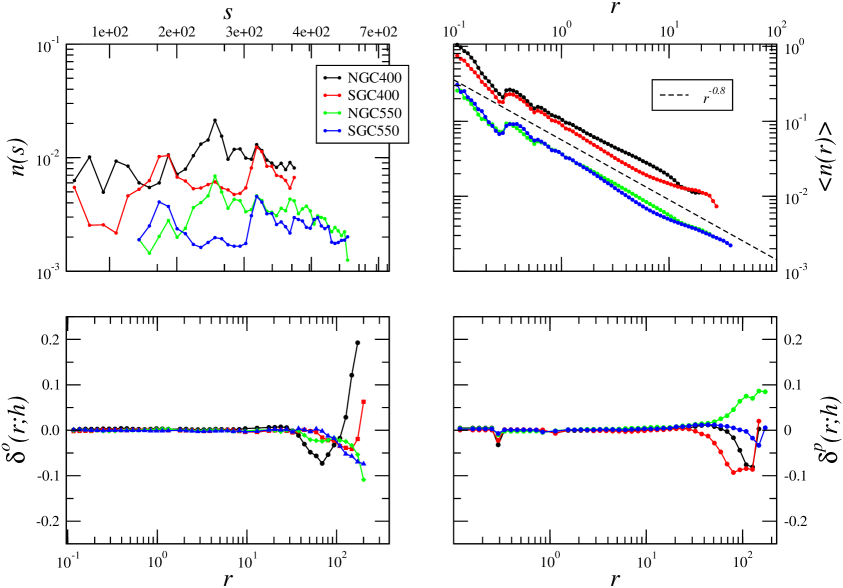
Figure 15: As for Fig.11 but for the 4 VL samples of the 2dFGRS survey ($h=1$ Mpc/h).

The behaviours of the FS estimators of the conditional density in spheres and cylinders are reported in Fig.16. In this case we observe that there is almost a factor ten between the distance up to which we may compute the conditional density in spheres and in cylinders. Such a difference is due to the geometry of the sample, i.e. 2dFGRS cover a small solid angle in the sky but it is relatively deep. However the large scale behaviours of $\langle n^{p}(r;h)\rangle$ and of $\langle n^{o}(r;h)\rangle$ do not allow to make a reliable estimate of the large scales, i.e. $r>50$ Mpc/h, correlation exponent: from the one hand there are significant sample-to-sample fluctuations and from the other hand, as discussed above, if there occurs a change of slope at $\lambda_{*}\approx 20-40$ Mpc/h it is not possible to make a reliable estimation of the exponent with in the conditional density in cylinders.

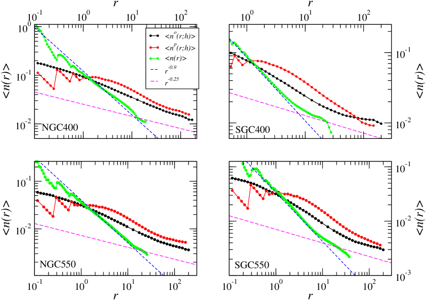
Figure 16: Behaviour of the conditional density computed in spheres and in cylinders of radius $h=1$ Mpc/h in several VL samples of the 2dFGRS survey.

4.3 The Two Micron All Sky Galaxy Redshift Survey

The various samples of the Two Micron All Sky Galaxy Redshift Survey (2MRS) samples (see Sect.A.3), that contains galaxy selected in the near infrared at low redshift and thus with small evolutionary and K-corrections, do not show any strong radial selection effect (see Fig.17). The conditional density, at small scales, shows a power-law behaviour that is similar to the one detected in the VL samples of SDSS and 2dFGRS. Even in this case it is not possible to investigate further the change of slope at large scales because of the limited size of the samples and the relatively small number of points contained.

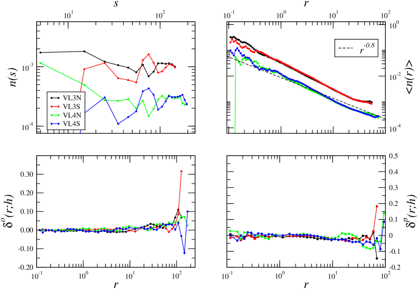
Figure 17: As for Fig.11 but for the 4 VL samples of the 2MRS survey ($h=1$ Mpc/h).

5 Discussion and Conclusions

The simplest statistical quantity to characterise spatial correlations of a point distribution is represented by the conditional density $\langle n(r)\rangle$. This gives the average number of points in a sphere of radius $r$ (or in a shell of thickness $\Delta r$ and radius $r$) centred in a distribution point [26]. The standard two point correlation function is related to the conditional density but it requires the additional estimation of the sample density $n_{0}$, as $\xi(r)=\langle n(r)\rangle/n_{0}-1$. This statistics gives a meaningful physical result only if the estimation of sample average represents a reliable estimation of the ensemble average density, i.e. only if the distribution is uniform well inside the sample volume. Therefore, in order to test whether a distribution is indeed uniform inside a given sample one should therefore study the conditional density and only if this show a scale independent behaviour one can then consider $\xi(r)$ to characterise correlation properties of small amplitude density fluctuations.

Given this situation the next problem we considered was to clarify which is the most suitable estimator of $\langle n(r)\rangle$. There are several studies discussing the problems related to the different estimators introduced in the literature (see, e.g., [25, 40, 26, 35]). They all compute the number of points in spherical volumes and the basic distinction is whether or not these volumes are fully included in the sample. The full shell (FS) estimator uses only complete spherical volumes, while non-FS estimators use volumes which are not completely included in the sample boundaries, by giving appropriate weights to them. It was argued in various previous works (see, e.g., [25, 26] and references therein) that the FS makes the most conservative estimation, limiting the analysis to the radius $R_{s}$ of the largest sphere fully contained in the sample volume: for deep surveys, when the survey solid angle is small, this can that can be much smaller than the maximum distance $R_{max}$ between two points. However, the advantage is that, when the statistical volume average is properly performed, i.e. for scales smaller than $R_{s}$, there are not unknown biases affecting the estimation.

Instead non-FS estimators, like the [36] the [38] and the [37] estimators, can reach scales of the order of $R_{max}$. However, for a generic distribution, they are affected on large scales, i.e. $R_{s}\leq r\leq R_{max}$ by strong finite size effects [25, 26]. We have shown, by considering the determination of non-FS estimators for several point distributions with a-priori know properties (see Sect.3), that this is indeed the case. For this reason we conclude that the claim of a transition toward uniformity by [19] is valid only under the assumption that the distribution is uniform inside the WiggleZ survey. Indeed, the WiggleZ having a complex angular and redshift selection function, does not represent a suitable sample for an analysis with a FS estimator which instead requires a contiguous volume corresponding to a uniform sampled sky area. In order to take into account these problems, the Rivolo [37] estimator was used by authors of the WiggleZ survey correlation analysis [19]. However, this estimator is affected, for a generic distribution, by an unknown bias and variance on large scales. For this reason the result obtained by [19] represent only a self-consistency test of the transition to homogeneity rather than a robust model-independent test of homogeneity itself. That is, if galaxy distribution is uniform at small scales., i.e. $r\approx 50$ Mpc/h, then with the Rivolo estimator is able to improve the estimation of the conditional density (or of $\xi(r)$) by taking into account the complicated selection function of the survey. However if galaxy distribution is not uniform by using the Rivolo estimator one cannot draw any definitive conclusion on the value of the large scale correlation exponent.

We have discussed in detail above that the FS estimator has another important limit: it can be applied only to samples which do not suffer for relevant radial and angular selection effects. Thus first of all one must use volume limited (VL) samples, that are not affected by the Malmquist bias [46], and then one should control that no other radial and/or angular selection effects are present in the samples. For what concerns the latter, the conservative procedure, that we have used in this paper, to take into account the inhomogeneous angular sampling is to limit the analysis only to that part of the sample where the angular completeness is $>90\%$ and as uniform as possible. This is not always possible and for instance catalogues like WiggleZ [3] or the first data release of the BOSS sample (i.e., SDSS DR9) [4] have a very inhomogeneous angular coverage of the sky, a fact that makes them unsuitable for a correlation analysis with the FS estimator.

Instead, the non FS estimators are able to correct selection effects by comparing data-data counts to the data-random points counts, where the random catalogues are characterised by the same radial and angular selection as the real data. This means that these random catalogues have the same radial counts $n(s)$ as the real data. However, this correction method is valid only for distributions which are uniform well inside the sample boundaries. In this way, one implicitly assumes that any departure of $n(s)$ from an almost constant behaviour on large scale is due a selection effect.

The conclusion of this discussion is that the non FS estimators should not be used to test whether a distribution is uniform inside a given as, for different reasons, they work under the assumption that a distribution is indeed uniform inside the given sample. There are then two open problems: (i) how to extend the analysis beyond $R_{s}$ and whether this is at all possible and (ii) how to identify and possibly quantify spurious radial selection effects in VL samples introduced by observational and/or physical reasons.

In order to reach separations of the order of $R_{max}$, i.e., of the order of the maximum distance between two points in the survey, with the FS estimator we have measured the conditional density in cylinders, included in the sample volume. The cylinders have a galaxy in their centre and are oriented along the LOS passing for that the centre point or orthogonally to it. In the former case we estimate $\langle n^{p}(r;h)\rangle$ and in the latter $\langle n^{o}(r;h)\rangle$. If there are no selection effects, redshift space distortion are negligible and the distribution is isotropic we expect $\langle n^{p}(r;h)\rangle\approx\langle n^{o}(r;h)\rangle\approx\langle n(r)\rangle$. Any radial dependent effect, such as spurious observational selection effects, intrinsic physical effects depending on distance (e.g., galaxy evolution, etc.) will alter this situation.

We have then measured the conditional density with the FS estimator in spherical volumes in several redshift surveys, i.e. the main galaxy sample of SDSS, the LRG-SDSS samples, the QSO-SDSS samples, the 2dFGRS samples and the 2MRS samples. We find in all samples that at small scales, i.e. $r\leq 20$ Mpc/h the exponent is $\gamma\approx 0.9$, while on large scales, in the SDSS VL samples which cover larger volumes, there is evidence of a change of slope, where we estimate $\gamma\approx 0.3$ in the range $20-100$ Mpc/h. For the case of the LRG sample we concluded further work is required to determine whether selection effects introduce a relevant bias in the measurement of its statistical properties. Indeed, although this shows a relatively small selection, i.e. $\delta^{p}(r)\approx 0.05$, this rapidly grows toward its boundary (i.e., $r\in[100,200]$ Mpc/h).

We have then used the determination of the conditional density by means of the FS cylinder method to constraint large scale selection effects in the data. In particular, we have introduced a new method, the gradient cylinder method (CGM), which is able to detect radial dependent selection effects in three dimensional galaxy samples without the assumption of spatial homogeneity of the underlying distribution. In practice, we define a normalised quantity along the LOS, $\delta^{p}(r;h)$, or perpendicularly to it $\delta^{o}(r;h)$, and we measure its amplitude and its dependence of the distance $r$. We have tested it in artificial samples with a priori known proprieties. We have shown, by considering artificial point distribution with known properties, that the CGM is able to correctly identify the selection effects that were introduced in the data. In particular, when $\delta^{p}(r;h)>0.1$ selection effects maybe strong enough to influence the behaviour of the conditional density measured with FS estimators in spheres. On the other hand we have also found that the conditional density is insensitive to moderate selection effects in the data.

We have applied the CGM method to the above mentioned redshift surveys. The main results is that almost in all samples we do not find a large radial dependence. The samples that are mostly influenced by these effects are the deeper VL samples of the SDSS and the LRG samples, where, at large scales $\delta^{p}(r;h)\approx 0.1-0.2$. Instead for the other VL samples of SDSS, for the 2dFGRS and the 2MRS samples we find $\delta^{p}(r;h)\approx\delta^{o}(r;h)\leq 0.1$. On the other hand, the QSO-DR7 samples are completely dominated by radial dependent effects (physical QSO evolution and luminosity selection effects) that it is not possible to make a reliable correlation analysis in these samples.

In summary we have introduced a new method to study large scales correlation properties of galaxy distribution and that allows to control redshift dependent selection effects. The application of these methods to forthcoming redshift surveys, like the extension of the SDSS [4], when they will cover a contiguous and large sky area, will be able to clarify the nature of galaxy correlations on scales $>100$ Mpc/h.

Appendix A The data

We briefly summarise the main properties of the redshift surveys for which we have analysed correlation properties.

A.1 SDSS

The SDSS [1] is currently the largest spectroscopic survey of extragalactic objects containing redshifts for more than 1,000,000 galaxies and 100,000 quasars. There are two independent parts of the galaxy survey in the SDSS: the main galaxy (MG) sample and the luminous red galaxy (LRG) sample.

A.1.1 The main galaxy sample

For the MG sample we have considered spectroscopic catalogue SDSS-DR7 (see [29] and the SDSS web site http://www.sdss.org). The spectroscopic survey covers an area of about 10,000 square degrees on the celestial sphere. The Petrosian apparent magnitude limit with extinction corrections for the galaxies is 17.77 in the $r$-filter and photometry for each galaxy is available in five different bands. A detailed discussion of the spectroscopic target selection in the SDSS MG sample can be found in [28].

We have constructed several volume limited (VL) samples that are unbiased for the selection effect related to the cuts in the apparent magnitude. To this aim we have applied the standard procedure described, for instance in [42] by considering the following steps (we refer the interested reader to [9] for more details).

• We selected only the galaxies from the MG sample.

• We considered galaxies in the redshift range $10^{-4}\leq z\leq 0.3$ with redshift confidence $z_{conf}\geq 0.35$.

• We applied the apparent magnitude filtering condition $m_{r}<17.77$ [28].

• We considered galaxies in the angular region limited, in the SDSS internal angular coordinates, by $-33.5^{\circ}\leq\eta\leq 36.0^{\circ}$ and $-48.0^{\circ}\leq\lambda\leq 51.5^{\circ}$.

• We do not use corrections for the redshift completeness mask or for fiber collision effects. Both are estimated to be small.

• We computed the metric distances $r(z)={c\over H_{0}}\int_{1/(1+z)}^{1}{1\over y\sqrt{0.3/y+0.7y^{2}}}$ using the standard cosmological parameters, i.e., $\Omega_{M}=0.3$ and $\Omega_{\Lambda}=0.7$. Results are given in units of $h$ defined as $H_{0}=$100 h km/sec/Mpc.

• We computed absolute magnitudes $M_{r}$ using Petrosian apparent magnitudes in the $m_{r}$ filter corrected for Galactic absorption and we used standard K-correction from the VAGC data .

• Details of the VL samples are reported in Tab.1.

VL sample	$R_{min}$	$R_{max}$	$M_{min}$	$M_{max}$	N
VL1	50	200	-18.9	-21.1	73810
VL2	100	300	-19.9	-22.0	110570
VL3	125	400	-20.5	-22.2	129974
VL4	150	500	-21.1	-22.4	94179
VL5	200	600	-21.6	-22.8	51697
VL6	70	450	-20.8	-21.8	112860

Table 1: Main properties of the obtained SDSS VL samples: $R_{min}$, $R_{max}$ (in Mpc/h) are the chosen limits for the metric distance; ${M_{min},\,M_{max}}$ define the interval for the absolute magnitude in each sample and $N$ is the number of galaxies included in the sample.

A.1.2 The luminous red galaxy sample

The selection of the LRG galaxies is discussed in [30] while the construction of the different sub-samples considered here is described in detail by [31]. Briefly, we focus on the so-called DR7-Dim which is limited by $0.16<z<0.36$. Indeed, for $z>0.36$ there is a clear selection effect due to the passage of the 4000 A break into the $r$ band [31]. This corresponds to the sharp decrease of the redshift counts for $z>0.36$.

The limits for the DR7-Dim sample are: $R_{min}=465$ Mpc/h and $R_{max}=1002$ Mpc/h. The limits in R.A. $\alpha$ and Dec. $\delta$ considered are chosen in such a way that (i) the angular region does not overlap with the irregular edges of the survey mask and (ii) the sample covers a contiguous sky area. Thus we have chosen: $\alpha_{min}=130^{\circ}\leq\alpha\leq\alpha_{max}=240^{\circ}$; $\delta_{min}=0^{\circ}\leq\delta\leq\delta_{max}=50^{\circ}$ . The absolute magnitude is constrained in the range $M\in[-23.2,-21.2]$. With these limits we find $N=41,833$ galaxies covering a solid angle $\Omega=1.471$ sr.

As we are interested in determining the role of selection effects, we have also considered the LRG sample SDSS-Full limited at $z<0.4$, containing $N=65,470$ galaxies.

A.1.3 The quasar sample

We have considered fifth edition of the SDSS quasar (QSO) catalogue described in [32] whose main part consists of a contiguous area of about 7,600 deg² in the North Galactic Pole. The details of the construction of the QSO catalogue are presented in [32] (and references therein). In this paper we focus on a same sub-sample analysed by [20, 21] whose main characteristics are:

• a redshift range $z\in[1.0,1.8]$

• an angular region limited by $130^{\circ}\leq\alpha\leq 235^{\circ}$ and $0^{\circ}\leq\delta\leq 60^{\circ}$

• The $i-$band apparent magnitude limit is $i\leq 19.0$.

The sample constructed in this way is ML and contains N=18,722 QSO. We have then constructed a VL sample by imposing the additional limits in distance, $R_{max}\leq 4545$ Mpc/h, and absolute magnitude, $M_{min}=-26.0$ and selecting in this way N=6351 objects.

A.2 The Two-degree Field Galaxy Redshift Survey

The Two-degree Field Galaxy Redshift Survey (2dFGRS) [2] measured redshifts for more than $220,000$ galaxies in two strips, one in the Southern Galactic Cap (SGC) and the other in the Northern Galactic Cap (NGC). As for the SDSS survey, we have constructed some VL samples (more details can be found in [12]):

• The apparent magnitude corrected for galactic extinction in the $b_{J}$ filter is limited to $14.0<b_{J}<19.45$.

• We selected two rectangular regions: in the SGC there is a slice of size $84^{\circ}\times 9^{\circ}$ limited by $-33^{\circ}<\delta<-24^{\circ}$, $-32^{\circ}<\alpha<52^{\circ}$, while the NGC slice is smaller, i.e., $60^{\circ}\times 6^{\circ}$, with limits $-4^{\circ}<\delta<2^{\circ}$, $150^{\circ}<\alpha<210^{\circ}$

• Galaxies have redshifts in the range $0.01\leq z\leq 0.3$.

• We did not use a correction for the redshift-completeness mask and for the fiber collision effects, which are negligible in the region we considered.

• We applied K-correction $K(z)$ as in [12].

• Details of the VL samples are reported in Table 2.

VL sample	$R_{min}$	$R_{max}$	$M_{min}$	$M_{max}$	$N_{g}$
SGC400	100	400	-20.8	-19.0	29373
NGC400	100	400	-20.8	-19.0	23208
SGC550	150	550	-21.2	-19.8	26289
NGC550	150	550	-21.2	-19.8	18030

Table 2: Main properties of the obtained VL samples. $R_{min}$, $R_{max}$ are the chosen limits for the metric distance; ${M_{min},\,M_{max}}$ are the corresponding limits in the absolute magnitude; $N_{g}$ is the number of galaxies in the sample.

A.3 The Two Micron All Sky Galaxy Redshift Survey

The Two Micron All Sky Galaxy Redshift Survey (2MRS) contains sample of 44599 galaxies with $K_{s}<11.75$ mag and $|b|>5^{\circ}$ ($>8^{\circ}$ towards the Galactic Centre) [43]. This sample of the near-infrared all-sky galaxies contains 44599 homogeneously selected spectral galaxy redshifts. From the ML sample we construct 8 (VL) samples (see Tab.3) 4 in the Northern (N) and 4 in the Southern hemispheres. No additional correction have been used because the sample is at low-redshift and because K-corrections are small in the near infrared.

	$R_{max}$	$M_{K}$	N	$\Lambda$
VL1N	50	-21.87	1845	1.51
VL2N	100	-23.39	4768	2.27
VL3N	150	-24.27	6133	3.26
VL4N	200	-24.95	3741	5.64
VL1S	50	-21.87	936	1.93
VL2S	100	-23.39	4925	2.23
VL3S	150	-24.27	5923	3.28
VL4S	200	-24.95	4015	5.38

Table 3: Parameters of the considered VL samples of 2MRS galaxies: $R_{max}$ limiting of the considered VL samples of 2MRS galaxies: $M_{K}$ limiting absolute magnitude in the $K_{s}$ filter, $N$ - number of objects and $\Lambda$ is the mean distance between nearest neighbours in $Mpc/h$.

References

- [1] York, D., et al., York, D., et al., The Sloan Digital Sky Survey: Technical Summary, Astron.J., 120, (2000), pg.1579
- [2] Colless M., Maddox S., Cole S., et al., The 2dF Galaxy Redshift Survey: spectra and redshifts Mon.Not.R.Acad.Soc., 328, (2001), pg.1039
- [3] Drinkwater M. J., et al., The WiggleZ Dark Energy Survey: survey design and first data release Mon.Not.R.Acad.Soc., 401, (2010), pg.1429
- [4] Ahn, S.-I. C. C. P., Alexandroff, R., Allende Prieto, C., et al., The Ninth Data Release of the Sloan Digital Sky Survey: First Spectroscopic Data from the SDSS-III Baryon Oscillation Spectroscopic Survey, Astrophys.J. Suppl. 203, (2012), pg.21
- [5] Sylos Labini F., Montuori, M. Pietronero, L. Scale-invariance of galaxy clustering Phys.Rep. 293, (1998), pg.61
- [6] Hogg D.W. et al., Cosmic Homogeneity Demonstrated with Luminous Red Galaxies Astrophys.J. 264, (2005), pg.54
- [7] Joyce M., Sylos Labini F., Gabrielli A., et al., Basic properties of galaxy clustering in the light of recent results from the Sloan Digital Sky Survey Astron,Astrophys 443, (2005), pg.11
- [8] Sylos Labini, F., Vasilyev, N.L., Baryshev, Yu. V., Power law correlations in galaxy distribution and finite volume effects from the Sloan Digital Sky Survey Data Release Four Astron,Astrophys 465, (2007), pg.23
- [9] Sylos Labini, F. Vasilyev, N.L., Baryshev, Y.V., Breaking the self-averaging properties of spatial galaxy fluctuations in the Sloan Digital Sky Survey - Data release six Astron,Astrophys 465, (2009), pg.17
- [10] Sylos Labini, F., et al., Absence of self-averaging and of homogeneity in the large-scale galaxy distribution Europhys.Lett. 88, (2009), pg.49001
- [11] Sylos Labini, F., Vasilyev, N.L., Baryshev, Y.V., Persistent fluctuations in the distribution of galaxies from the Two-degree Field Galaxy Redshift Survey Europhys.Lett. 85, (2009), pg.29002
- [12] Sylos Labini, F., Vasilyev, N.L., Baryshev, Yu. V., Large-scale fluctuations in the distribution of galaxies from the two-degree galaxy redshift survey Astron,Astrophys 496, (2009), pg.7
- [13] Antal, T., Sylos Labini, F., Vasilyev, N.L., Baryshev, Yu. V., Galaxy distribution and extreme-value statistics Europhys.Lett. 88, (2009), pg.59002
- [14] Sylos Labini F., Inhomogeneities in the universe Class.Quantum.Grav. 28, (2011), pg.164003
- [15] Bagla J., Yadav J., Seshadri T., Fractal dimensions of a weakly clustered distribution and the scale of homogeneity Mon.Not.R.Acad.Soc., 390, (2008), pg.829
- [16] Nabokov, N. V.& Baryshev, Yu. V., Method for analysing the spatial distribution of galaxies on gigaparsec scales. I. Initial principles Astrophysics 53, (2010), pg.91
- [17] Nabokov, N. V.& Baryshev, Yu. V., Method for analysing the spatial distribution of galaxies on gigaparsec scales. II. Application to a grid of the HUDF-FDF-COSMOS-HDF surveys Astrophysics 53, (2010), pg.101
- [18] Einasto M., et al., The Sloan Great Wall. Morphology and Galaxy Content Astrophys.J. 736, (2011), pg.51
- [19] Scrimgeour M. et al., The WiggleZ Dark Energy Survey: the transition to large-scale cosmic homogeneity Mon.Not.R.Acad.Soc., 425, (2012), pg.116
- [20] Clowes R. G., Harris K. A., Raghunathan S., Campusano L. E., Soechting I. K., Graham M. J., A structure in the early Universe at z=1.3 that exceeds the homogeneity scale of the R-W concordance cosmology Mon.Not.R.Acad.Soc., 429, (2013), pg.2910
- [21] Nadathur S. Seeing patterns in noise: Gigaparsec-scale ‘structures’ that do not violate homogeneity Mon.Not.R.Acad.Soc., 434, (2013), pg.398
- [22] Shen S. et al., Quasar Clustering from SDSS DR5: Dependences on Physical Properties Astrophys.J., 680 (2008), pg. 169
- [23] Ross N.P. et al., Clustering of Low-Redshift () Quasars from the Sloan Digital Sky Survey Astrophys.J 697 (2009), pg.1634
- [24] Wu K.K.S, Lahav O., Rees M., The large-scale smoothness of the Universe Nature, 397, (1999), pg.225
- [25] Kerscher, M., The geometry of second-order statistics - biases in common estimators Astron,Astrophys 333, (1999), pg.333
- [26] Gabrielli A., Sylos Labini F., Joyce M., Pietronero L., Statistical Physics for Cosmic Structures Springer Verlag, Berlin (2005)
- [27] Croton, D.J., et al., The many lives of active galactic nuclei: cooling flows, black holes and the luminosities and colours of galaxies Mon.Not.R.Acad.Soc., 365, (2006), pg.11
- [28] Strauss, M.A., et al., Spectroscopic Target Selection in the Sloan Digital Sky Survey: The Main Galaxy Sample Astronom.J. 124, (2002), pg.1810
- [29] Adelman-McCarthy J., et al., The Sixth Data Release of the Sloan Digital Sky Survey Astrophys.J.Suppl. 175, (2008), pg.297
- [30] Eisenstein, D.J., et al. et al., Spectroscopic Target Selection for the Sloan Digital Sky Survey: The Luminous Red Galaxy Sample Astronom.J. 12, (2001), pg.2267
- [31] Kazin E. et al.,, The Baryonic Acoustic Feature and Large-Scale Clustering in the Sloan Digital Sky Survey Luminous Red Galaxy Sample Astrophys.J. 710, (2010), pg.1444
- [32] Schneider D. P., et al., The Sloan Digital Sky Survey Quasar Catalogue. V. Seventh Data Release Astronom.J. 139, (2010), pg.2360
- [33] Norberg P., Baugh C.M., Gaztanaga E., Croton D.J., Statistical Analysis of Galaxy Surveys - I. Robust error estimation for 2-point clustering statistics Mon.Not.R.Acad.Soc., 369, (2009), pg.19
- [34] Sylos Labini, F., Vasilyev, N.L., Baryshev, Y.V., Lopez-Corredoira M. Absence of anti-correlations and of baryon acoustic oscillations in the galaxy correlation function from the Sloan Digital Sky Survey DR7 Astron,Astrophys 505, (2009), pg.981
- [35] Sylos Labini, F., Vasilyev, N.L. Extension and estimation of correlations in cold dark matter models Astron,Astrophys 477, (2008), pg.381
- [36] Davis, M., Peebles, P.J.E., A survey of galaxy redshifts. V - The two-point position and velocity correlations Astrophys.J. 465, (1983), pg.267
- [37] Rivolo A.R., The two-point galaxy correlation function of the Local Supercluster Astrophys.J. 301, (1986), pg.70
- [38] Landy S. D., Szalay A. Bias and variance of angular correlation functions Astrophys.J. 412, (1993), pg.64
- [39] Hamilton A.J.S., Toward Better Ways to Measure the Galaxy Correlation Function Astrophys.J. 417, (1993), pg.19
- [40] Kerscher M., Szapudi I., Szalay A. S. A Comparison of Estimators for the Two-Point Correlation Function Astrophys.J. 535, (2000), pg.L13
- [41] Feldman, H.A., Kaiser, N., Peacock, J.A. Power-spectrum analysis of three-dimensional redshift surveys Astrophys.J. 426 (1994), pg.23
- [42] Zehavi, I. et al., The Luminosity and Colour Dependence of the Galaxy Correlation Function Astrophys.J. 630, (2005), pg.1
- [43] Huchra J. et al., The 2MASS Redshift Survey—Description and Data Release Astrophys.J.Suppl 199, (2012), pg.26
- [44] Sylos Labini, F. Baryshev, Y.V., Testing the Copernican and Cosmological Principles in the local universe with galaxy surveys J.Cosm.Astrop.Phys., 06, (2010), 021
- [45] Loveday, J., Evolution of the galaxy luminosity function at z 0.3 Mon.Not.R.Acad.Soc., 347, (2004), 601
- [46] Baryshev Yu.V. & Teerikorpi P., Fundamental Questions of Practical Cosmology Springer, Dordrecht Heidelberg London New York, (2012)