Scalable Analytics over Distributed Time-series Graphs using GoFFish

Abstract

Graphs are a key form of Big Data, and performing scalable analytics over them is invaluable to many domains. As our ability to collect data grows, there is an emerging class of inter-connected data which accumulates or varies over time, and on which novel analytics – both over the network structure and across the time-variant attribute values – is necessary. We introduce the notion of time-series graph analytics and propose Gopher, a scalable programming abstraction to develop algorithms and analytics on such datasets. Our abstraction leverages a sub-graph centric programming model and extends it to the temporal dimension using an iterative BSP (Bulk Synchronous Parallel) approach. Gopher is co-designed with GoFS, a distributed storage specialized for time-series graphs, as part of the GoFFish distributed analytics platform. We examine storage optimizations for GoFS, design patterns in Gopher to leverage the distributed data layout, and evaluate the GoFFish platform using time-series graph data and applications on a commodity cluster.

I Introduction

With the proliferation of ubiquitous physical devices (e.g. urban monitoring, smart power meters) and virtual agents (e.g. Twitter feeds, Foursquare check-ins) that sense, monitor and track human and environmental activity, data is streaming more continuously and is intrinsically interconnected. Two defining characteristics of such datasets, endemic to both the Internet of Things [1] and Social Networks, are the temporal or time-series attributes and the topological relationships that exist between them. Such datasets that imbue both these temporal and graph features have not been adequately examined from the perspective of scalable Big Data management and analysis, even as they are becoming pervasive.

Graph datasets with temporal characteristics have been variously known in literature as temporal graphs [2], kineographs [3], dynamic graphs [4] and time-evolving graphs [5]. Temporal graphs capture the time variant network structure in a single graph by introducing a temporal edge between the same vertex at different moments. Others construct graph snapshots at specific change points in the graph structure. In particular, kineographs deal with graph that exhibit high dynamism. In this paper, we focus on a related class of time-series graphs which we define to be graphs whose network topology is slow-changing but whose attribute values associated with vertices and edges change (or are generated) more frequently. As a result, we have a series of graphs, each of whose vertex and edge attributes capture the instantaneous state of a system at a point in time (e.g. 2013-07-14 15:00 PST), or the cumulative states of the system over time durations (e.g. 2013-07-14 15:00 PST – 15:05 PST), but whose numbers of, and connectivity between, vertices and edges are less dynamic. Each graph in the time-series is an instance, while the slow changing topology is a template (Fig. 1).

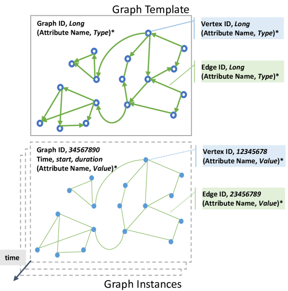
Figure 1: Time-series graph collection. Template captures static/slow-changing topology and attribute names. Instances record temporally variant attribute values for this template.

Many emerging “Big Data” datasets can be captured using such a time-series graph model. For e.g., when we consider images captured by a network of traffic or surveillance cameras in a large city like Los Angeles or London, these cameras themselves are inter-connected by the roads that link them (i.e. the graph topology) and their location changes less often. On the other hand, the periodic data that they generate after image processing, such as vehicle license IDs at the vertices and the current travel-time on edges, form a time-series graph. Similarly, we can construct time-series graphs out of social network feeds (friend network forms the “slow changing” topology while tweets or posts form the instances) or even Internet trace-route statistics (Internet IPs on network hops form the topology while current latency and bandwidth form instances). As such, these datasets are expected to have over $O(10^{6})$ vertices, $O(10^{7})$ edges, and $O(10^{4})$ time points.

Many innovative analytics applications can leverage the topological and temporal information that a time-series graph representation provides. While some are a temporal extension of existing algorithms, others are more novel. For e.g., we can extend the Dikstra’s shortest path algorithm to a temporal version over a road network with snapshots of historical traffic conditions accumulated every 5-min. We start traversing at the source vertex of a graph instance and use its travel times in estimating the shortest path. But after traveling 5-mins and reaching the temporal boundary of that graph instance (e.g. we determine that the next position cannot be in the current graph instance due to traffic conditions such as the average speed), we switch over to the next graph instance in the time-series with traffic information on the next 5-mins, and resume traversal. This gives us concentric waves of traversals. The space of such large-scale temporal graph analytics applications is rich, ranging from studying time-evolving social network communities to Internet router bottlenecks.

In our recent work [6], we extended the idea of scalable vertex centric Bulk Synchronous Parallel (BSP) [7] graph programming model, championed by Google’s Pregel [8] and implemented by others like Giraph [9, 10], into a sub-graph centric model, Gopher, that was targeted at commodity cluster and Cloud platforms. The platform operated on a single graph and significantly out-performed Giraph in our benchmarks. In this paper, we further expand Gopher to support time-series graph analysis in distributed environments. Specifically, we propose structured programming abstractions for large-scale analytics across multiple graphs using an iterative BSP model. In addition, we couple this with a distributed storage model optimized for time-series graphs called Graph-oriented File System (GoFS), that we introduce here. GoFS partitions the graph based on topology, groups instances over time on disk, and allows attribute-value pairs to be associated with the vertices and edges of the instances. In particular, GoFS is designed to scale out for common data access patterns over time-series graphs, and this data layout is intelligently leveraged by Gopher during execution. Gopher and GoFS are part of the GoFFish graph analytics framework.

We make the following specific contributions in this paper:

1. We propose a time-series graph model and an iterative Bulk Synchronous Parallel programming abstraction for composing sub-graph centric analytics over this data model (§ III–IV);

2. We discuss design patterns for classes of time-series graph analytics, and present a distributed graph storage layout optimized for these access patterns (§ V);

3. We implement the iterative BSP abstraction and distributed layout as part of the GoFFish analytics platform, and present an empirical evaluation of the abstractions and optimizations for sample graph algorithms and datasets (§ VI).

II Related Work

With the advent of truly Big data sources with graph oriented structures in modern computing, there has been a renewed focus on scalable and accessible platforms for their analysis. Current approaches can be separated into three categories; Map/Reduce frameworks, Bulk Synchronous Parallel (BSP) frameworks, and online processing systems. Our effort is focused on BSP and for offline queries. While many of the mature frameworks offer complete distributed solutions, with fault tolerance and performance guarantees, GoFFish focuses on exploring novel graph processing abstractions that are easy to use and can be scaled. In this paper, we do not reinvent well understood reliability and recovery approaches.

Map/Reduce [11] has become a de facto abstraction for large data analysis, and has been applied to graph data as well [12]. However its use for general purpose graph processing can lead to both performance and usability concerns [13]. Iterative versions of Map/Reduce have been proposed to address some of the limitations of the original abstraction [14]. Further extensions have added features for aggregation [15] and SQL-like queries, but these are ill suited for graph processing, which is better served through a message passing model [16]. However, it is possible to improve upon these frameworks through graph-specific programming models. GoFFish is in this vein, combining prior work on BSP graph frameworks with timeseries analysis using a sub-graph centric model [6, 17].

Google recently proposed the Pregel model [8] of vertex centric programming for large scale graph processing, which also has similarities with GraphLab [18]. The Pregel model allows the programmer to implement algorithms from the point of view of a single vertex which remarkably simplifies the programming model for a large class of graph algorithms and allows for much simpler and quicker development. Further, Pregel’s execution model is based on BSP [7], where computation is done through a series of barriered iterations called supersteps. This model of parallel computing eliminates concerns of deadlocks and data races common in asynchronous systems [16]. While the original BSP model fell out of favor in parallel computing due to the large cost of superstep synchronization, for large graphs, one can balance machine-level vertex computation load and use hierarchical synchronization to mitigate this synchronization overhead. Further, with the push toward commodity hardware and Cloud infrastructure, the emphasis is more on scalability than performance on HPC hardware.

The vertex-centric BSP model has been adopted by a variety of frameworks [17] like Giraph [9], Hama and GPS [10] that implement improvements on the original idea. Giraph is currently the popular framework in this space, being adopted by Facebook for large scale graph analysis on their network data. GPS is a vertex-centric framework with support for dynamic repartitioning of the graph between hosts. Many of these frameworks offer engineering optimizations to improve performance and simplify programming. These include master compute methods, send- and receive-side message aggregation, dynamic partition balancing, and message as well as graph memory compression techniques. Many of these optimizations focus on reducing the effective number of messages passed around the system, both in memory and on the network. This emphasis is because the number of messages correspond roughly to the number of edges for a large class of graph algorithms. On large graphs with power law out-degree distributions, the number of generated messages can flood both memory and network. However, part of the problem lies not in engineering solutions but in that these frameworks do not deviate much from Pregel’s original vertex centric model. This limits more significant optimizations possible within them.

Our earlier work on GoFFish improves on Pregel by proposing a subgraph centric model rather than a vertex centric one [6]. For a large number of algorithms the amount of work performed per vertex is so negligible that the overhead of massive parallelism can outweigh the benefits. By using a subgraph as a unit of computation, we show that the efficiency of every worker is increased, and the number of messages the framework must handle is dramatically reduced, since it is more a function of the number of unique edges between sub-graphs that span partitions, rather than between vertices. This also results in effectively more work being performed in each superstep, and thus requires fewer supersteps, with associated synchronization overhead, to complete the application.

This comes at the cost of marginally increasing the complexity of the programming model, mixing features of vertex centric and shared-memory graph abstractions. But for many applications the performance and scalability improvements may be worth the costs. In this article, we further expand upon this to support time-series graphs, which Pregel does not natively support and is punitive to implement naïvely using the vertex centric approach. We also investigate a novel distributed data storage that is optimized for time-series graphs. While Pregel does not prescribe any data storage, the Apache Giraph implementation of Pregel retains the tuple-based HDFS for storing graphs, which impacts initial loading from disk to memory even for single graphs.

Online processing systems such as Kineograph [3] and Trinity [19] are graph processing models that focus heavily on the analysis of streaming information, and are thus purpose built for time evolving graphs. These systems are able to process an large quantity of information with timeliness guarantees. Kineograph’s approach can also potentially support time-series graphs using consistent snapshots with an epoch commit protocol. Traditional graph algorithms are then run on top of each static snapshot. However, GoFFish does not aim to provide streaming or online graph processing services, but rather more traditional offline bulk processing on large datasets. Dealing with dynamic topologies and streaming data is not within the scope of this paper.

III Analytics over Time-series Graphs

III-A Time-series Graphs

Time-series graphs can be considered as snapshots of a graph recorded over time (Fig. 1). We define a collection of time-series graphs as $\Gamma=\langle\widehat{G},G\rangle$, where $\widehat{G}$ is called a graph template that is the time invariant topology, and $G$ is an ordered set of graph instances, capturing time-variant values. $\widehat{G}=(\widehat{V},\widehat{E})$ gives the set of vertices, $\hat{v}_{i}\in\widehat{V}$, and edges, $\hat{e}_{j}\in\widehat{E}:\widehat{V}\rightarrow\widehat{V}$, common to all instances. The graph instance $g^{t}\in G$ at timestamp $t$ is given by $(V^{t},E^{t},t)$ where $V$ and $E$ capture the vertex and edge values for $\widehat{V}$ and $\widehat{E}$ at time $t$, $|V^{t}|=|\widehat{V}|$ and $|E^{t}|=|\widehat{E}|$. The set $G$ is ordered in time.

Vertices and edges in the template have a defined set of typed attributes, $\mathbb{A}(\widehat{V})=\{id,\alpha_{1},\ldots,\alpha_{m}\}$ and $\mathbb{A}(\widehat{E})=\{id,\beta_{1},\ldots,\beta_{n}\}$ respectively. All vertices and edges share the same set of attributes with $id$ being one of the unique identifier attribute. These similar attributes are also present in the instances, except for the $id$ attribute, which is set in the templateThus each vertex $v^{t}_{i}\in V^{t}$ for a graph instance $g^{t}$ at time $t$ has a set of attribute values $\{\hat{v}_{i}.id,v_{i}^{t}.\alpha_{k},\ldots,v_{i}^{t}.\alpha_{m}\}$, and each edge $e^{t}_{j}\in E^{t}$ has attribute values $\{\hat{e}_{j}.id,e_{j}^{t}.\beta_{l},\ldots,e_{j}^{t}.\beta_{n}\}$,

A slow changing graph topology can be captured using the special isExists attribute flag that allows us to simulate the appearance/disappearance of vertices or edges throughout the time-series.

III-B Sample Applications

Analytics over individual graphs fall broadly into traversal (e.g. shortest path under changing conditions), centrality detection (e.g. betweenness centrality at different points in time) and clustering algorithms (e.g. evolution of community), among others. Applications over time-series graphs expand on these possibilities.

Centrality detection algorithms form a class of applications where the state of a vertex is analyzed in raport with the rest. Example applications include the page rank algorithm where each vertex’s rank relative to the other vertices’ rank is analyzed at each time snapshot. Since each graph instance contains all the information required to determine if a vertex is present in a path, at a particular moment, such analytics can operate on each instance independently. In that sense, they are similar to algorithms for individual graphs, except that they are repeated for each graph instance.

Clustering algorithms discover the existence of localized, time-evolving patterns. While each pattern can be identified independently for each instance, the individual results need to be aggregated at the end of the execution to get the global view. Applications that can pe placed in this category range from studies on the PageRank stability over time to analyzing the dynamics of a person’s social network and identifying frequent clusters in gene expression networks. Here, the application initially operates on each instance independently, but has to eventually perform an aggregation or analysis that spans the synthesized result from each instance.

Traversal algorithms show a linear dependence between instances as information gathered in the past drives traversals in the future. The shortest path over time-varying traffic conditions, presented in § I, falls in this space, and can be applied to network packet tracing or meme propagation. Further, this class includes minimum spanning trees to determine the optimal route for patrolling, and epidemiological studies to find the time for a disease to spread. Here, there is either a strict sequential dependence between one instance and its predecessor, or using information from a prior instance will help efficiently localize the search on the next.

III-C Design Patterns for Graph Analytics over Time

Based on these sample classes of algorithm we can synthesize three types of composition patterns for temporal graph analytics. These are illustrated in Fig. 2 and described next.

1. Analysis over every graph instance is independent. The result from the application is just a union of results from each graph instance;

2. Graph instances are eventually dependent. Each instance can execute independently but results from all instances need to be aggregated or summarized to produce the final result;

3. Graphs instances are sequentially dependent. Here, analysis over a graph instance cannot start (or, as a variation, complete) before the results from the previous graph instance are available.

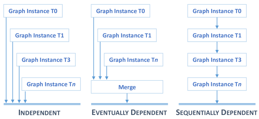
Figure 2: Design patterns for analytics on time-series graphs.

These patterns have two purposes in mind: make it easy for users to design common time-series graph analytics, and make it possible to efficiently scale them in a distributed environment. In the abstraction (§ IV) and evaluation sections (§ VI) we show exemplar applications mapped to these three patterns and empirically analyze them.

The independent pattern is similar to a Parallel For-Each construct. It allows concurrent execution over each graph instance with the parallelism that can be ideally exploited being equal to the number of graph instances.

The eventually dependent pattern captures the Fork-Join paradigm. This brings in additional synchronization capability for aggregation without compromising the parallelism. Pipelining can be facilitated if the pattern is extended to an “incremental” join where the Merge step starts as soon as the first graph instance completes, and ends when the last instance has finished executing.

The sequentially dependent pattern is a traditional sequential execution model. While it does not offer concurrency across time (i.e. instances), as we shall see, the subgraph centric BSP abstraction allows for spatial concurrency across vertices within a graph instance.

These models are not meant to be a comprehensive list and serve as the building blocks to help construct a large class of applications while retaining concurrency. While they can be incrementally extended to more complex patterns, e.g., monotonic dependency (a relaxation of sequential dependency), random access across instances, etc. we omit discussing these cases in this paper in the interests of being concise.

IV Programming Time-series Graph Analytics

In developing abstractions to fit the design patterns from § III, we build upon our recent work on sub-graph centric programming abstractions targeted at distributed programming over single graphs. We first present this initial model and then extend it with our novel iterative BSP model, along with several time-series graph algorithms mapped to it.

IV-A Sub-graph Centric Programming Abstraction

A sub-graph centric distributed programming abstraction defines the graph application logic from the perspective of a single sub-graph within a partitioned graph. A graph $G=(V,E)$ is partitioned into $n$ partitions, $\langle P_{1}=(V_{1},E_{1}),\cdots,P_{n}=(V_{n},E_{n})\rangle$ such that $\bigcup\limits_{i=1}^{n}V_{i}=V$, $\bigcup\limits_{i=1}^{n}E_{i}=E$, and $\forall i\neq j:V_{i}\cap V_{j}=\varnothing$, i.e. a vertex is present in only one partition, and all edges appear in one partitions, with the exception being “remote” edges that can span two partitions; $R_{i}=\{e_{p}|e_{p}\in E_{i}\text{ and }\forall e_{p}:v_{q}\rightarrow v_{r},v_{q}\in V_{i}\text{ and }v_{r}\not\in V_{i}\}$, if the edges are directed. If undirected, then either the source or the sink vertex is present is another partition. Conversely, “local” edges for a partition are those edges that are not remote; $L_{i}=\{e_{p}|e_{p}\in E_{i}\text{ and }\forall e_{p}:v_{q}\rightarrow v_{r},\text{ both }v_{q},v_{r}\in V_{i}\}$. Typically, partitioning tries to ensure that the number of vertices, $|V_{i}|$, is equal across partitions and the total number of remote edges, $\sum_{i=1}^{n}|R_{i}|$, is minimized.

Given this, a sub-graph within a partition is a maximal set of vertices that are connected through “local” edges. A partition $i$ may have between one and $|V_{i}|$ sub-graphs.

In sub-graph centric programming, the user defines an application logic as a Compute method that operates on a single sub-graph, independently. The method, upon completion, can exchange messages with other sub-graphs, typically those that share a remote edge with the source sub-graph. A single execution of the Compute method on all sub-graphs, each of which can execute concurrently, forms a superstep. Execution proceeds as a series of coordinated supersteps, executed in a Bulk Synchronous Parallel (BSP) model. Messages generated in one superstep are transmitted in “bulk” between supersteps, and available to the Compute of the destination sub-graph in the next superstep. Execution stops when all Compute methods Vote to Halt and there are no messages generated within a superstep. Fig. 3 illustrates this execution model.

The sub-graph centric programming abstraction is itself an extension to the vertex centric model, where the Compute logic is from the perspective of a single vertex [8]. Our prior work [6] shows the performance benefits of this innovation by limiting both the number of supersteps requiring costly synchronization and the number of messages exchanged. It also ease the programmability through the reuse of efficient, shared-memory graph algorithms within a single sub-graph.

IV-B Iterative BSP for Time-series Graph Programming

Sub-graph centric BSP programming offers natural parallelism across the graph topology. But it operates on a single graph instance. In a sense, a single BSP execution corresponds to one box in Fig. 2 that operates on a single graph instance. Here, we use BSP as a building block to define an iterative BSP (iBSP) abstraction that meets the design patterns proposed before. An iBSP application is a set of BSP steps, also referred to as timesteps since each operates on a single graph instance in time. While the BSP timestep itself can be opaque, we use the sub-graph centric abstraction consisting of supersteps as its constituent. In a sense, the timestep iteration acts as an “outer loop” while the supersteps over sub-graphs represent the “inner loop”. The execution order of the timesteps and the messages passed between them decides the iBSP application’s design pattern as in § III.

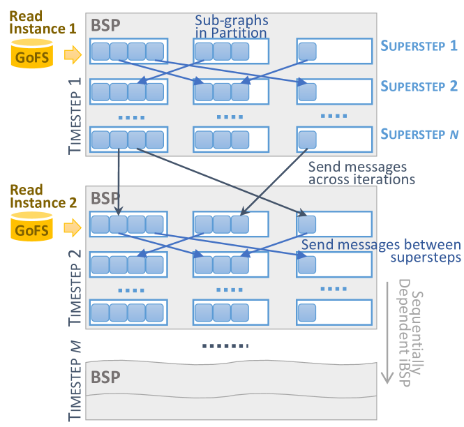
Figure 3: Iterative BSP programming model across time-series graph instances. Each BSP timestep operates on a single graph instance, and is itself decomposed into multiple supersteps as part of the sub-graph centric abstraction. Graph instance data access takes place at the start of each BSP timestep.

Orchestration and Concurrency. An iBSP application operates over a graph collection, $\Gamma$, which, as we defined earlier, is a list of time ordered graph instances. As before, the users implement a Compute method which is invoked on every sub-graph and for every graph instance. In case of an eventually dependent pattern, an optional Merge method is available for invocation after all instance timesteps complete.

For a sequentially dependent pattern, only one graph instance and hence BSP timestep is active at a time. The Compute method is called on all sub-graphs of the first instance to initiate the BSP, after the completion of whose supersteps, the Compute method is called on all sub-graphs of the next instance for the next timestep iteration, and so on till the last graph instance. So, while there is spatial concurrency across sub-graphs in a BSP superstep, each timestep iteration is itself sequentially executed after the previous. In case of an independent pattern, the Compute method can be called on any graph instance independently, as long as the BSP is run on each instance exactly once. The application terminates when all the BSP timesteps complete. Here, we have both spatial concurrency across sub-graphs and temporal concurrency across graph instances. An eventually dependent pattern is similar, except that the Merge method is called after the BSP timesteps complete on all instances of the graph collection. The parallelism is similar to the independent pattern, except for the merge BSP which has to be additionally executed last.

User Logic. The signatures of the Compute method and the Merge method, in case of an eventually dependent pattern, implemented by the user are follows. The parameters are passed to these methods by the execution framework.

Compute(SubgraphInstance sgInstance, int timestep, int superstep, Message[] msgs)
Merge(SubgraphTemplate sgTemplate, int superstep, Message[] msgs)

Here, the SubgraphInstance has the time variant attribute values of the corresponding graph instance for this BSP, in addition to the sub-graph topology that is time invariant. The timestep is a sequential number that corresponds to the graph instance’s index, while the superstep corresponds to the superstep number inside the BSP execution. If the superstep number is 1, it indicates the beginning of an instance’s execution. Hence, it offers a context for interpreting the list of messages, msgs. In case of a sequentially dependent application pattern, messages received when superstep=1 have arrived from its preceding BSP instance upon its completion. Hence, it indicates the completion of the previous timestep, start of the next timestep and helps to pass the state from one instance to the next. If, in addition, the timestep=1, then this is the first BSP timestep and the messages are the inputs passed to the application. For an independent or eventually dependent pattern, messages received when the superstep=1 are application input messages since there is no notion of a previous instance. In cases where superstep>1, these are messages received from the previous superstep inside a BSP.

Message Passing. Besides message passing between sub-graphs in supersteps, supported by the sub-graph centric abstraction, the Compute and Merge methods can use these additional message passing and application termination constructs, depending on the design pattern. SendToNextTimeStep(Message msg), used in sequentially dependent pattern, passes message from a sub-graph to the next instance of the same sub-graph, available at the start of the next timestep. This can be used to pass the end state of an instance to the next instance. SendToSubgraphInNextTimeStep(long sgid, Message msg), is similar, but allows a message to be targeted to another sub-graph in the next timestep’s instance. SendMessageToMerge(Message msg) is used in the eventually dependent pattern by sub-graphs in any timestep to pass messages to the merge method, which will be available after all timesteps complete execution. VoteToHalt(), depending on context, can indicate the end of a BSP timestep, or the end of the iBSP application in case this is the last timestep of a sequentially dependent pattern. It is also used by the merge method to terminate the application.

Gopher Framework. Gopher is a distributed framework implementation of the sub-graph centric BSP abstraction [6], which has been extended for the proposed iterative BSP model. It supports the new user logic and messaging APIs mentioned above, and allows composition and distributed execution of iBSP applications based on the three design patterns. Gopher works in tandem with the GoFS distributed data storage for time-series graphs introduced next. This cooperation utilizes some of the computational concurrency offered by the abstractions while also leveraging the data locality present in GoFS.

IV-C Sample iBSP Application

Algorithm 1 shows a sequentially dependent iBSP application that locates a vehicle, based on its license place $\mathbb{V}$, within a road network and tracks the vehicle over time across multiple instances. The graph template is a road network, and the graph instances have vertex attributes with license plates of vehicles seen at the intersection, for the duration of that instance (e.g. $5mins$). The first timestep determines the vehicle’s location in the entire graph and traces it spatially across sub-graphs, using message passing across supersteps, it until it goes missing in the instance’s time duration. It then moves to the next timestep containing the instance for the next $5mins$, and resumes the traversal from the last known sub-graph location, using message passing between timesteps. The algorithm terminates once all instances are exhausted.

Algorithm 1 Temporal Path Traversal using iterative BSP

1:procedure Compute(Instance sgi, int iteration, int superstep, Message msgs[])

2:    searchRoots $\leftarrow\varnothing$ $\triangleright$ Vertices to begin search for $\mathbb{V}$ on

3:    if superstep = 1 then $\triangleright$ Initialize from previous iteration

4:         if iteration = 1 then $\triangleright$ Initialize from user input

5:             v $\leftarrow$ initial_location

6:             searchRoots.add(v)

7:         else$\triangleright$ Get the last vertex seen with the search value, $\mathbb{V}$, from the previous iteration timestep.

8:             v $\leftarrow(\operatorname*{arg\,max}_{m\in msgs}\{\text{m.TimeStamp}\})$.vertex

9:             searchRoots.add(v)

10:         end if

11:    else$\triangleright$ Process messages from previous superstep

12:         for all Message m in msgs do

13:             v $\leftarrow$ m.vertex

14:             searchRoots.add(v)

15:         end for

16:    end if$\triangleright$ Depth first search on sub-graph from last seen location

17:    $\langle$ remoteSet, foundLocs $\rangle\leftarrow$ DFS(sgi, searchDepth, $\mathbb{V}$) $\triangleright$ If DFS crosses to neighboring sub-graph, send message to remote sub-graph to continue search in next superstep

18:    for all $\langle$ remoteSG, remoteVertex $\rangle$ in remoteSet  do

19:         Message m $\leftarrow\langle$ remoteVertex $\rangle$

20:         SendToSubGraph(remoteSG, m)

21:    end for

22:    if Locations $\neq\varnothing$ then $\triangleright$ If current instance exhausted, continue search in next timestep

23:         for all $\langle$ vertex, TimeStamp $\rangle$ in remoteSet do

24:             $\triangleright$ Send last known location message to next instance of the same sub-graph

25:             Message m $\leftarrow\langle$ vertex, TimeStamp $\rangle$

26:             SendToNextTimeStep(vertex, TimeStamp)

27:         end for

28:    end if

29:    VoteToHalt( )

30:end procedure

31:

V Distributed Storage and Execution Patterns

Big data applications can quickly become I/O bound unless the data storage and layout on disk are well planned for the intended usage patterns. While advanced database schema planning has given way to flat, schema-free distributed storage using HDFS and no-SQL databases, the interconnected nature of graph datasets, with the additional temporal dimension considered here, pose challenges to tuple-based storage models.

We propose a Graph oriented File System (GoFS) for distributed storage of time-series graphs on commodity clusters or Cloud VMs, with spinning disks. GoFS is architected for the data access patterns associated with time-series graph analytics, though in effect, both the programming abstractions and the data layout were co-designed. The typical usage model of GoFS is by Gopher, which loads subgraphs in the local host’s graph partition, and scans through instances as part of the BSP timestep iterations. The key tenets observed in this co-design are to: maximize concurrent execution, minimize network data movement, reduce disk I/O, and increase the compute to I/O ratio. Given the write once/read many model of GoFS, we trade off data layout cost against improved runtime performance. These choices are reflected in the GoFS data layout design and Gopher runtime execution optimizations.

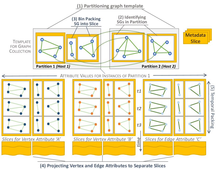
Figure 4: GoFS Data Layout. Top shows graph template partitioned and mapped to slices on two hosts. Bottom shows time-series graph instances on Host 1. Yellow boxes are slices.

V-A Partitioned Storage using Slices

GoFS can store multiple time-series graph collections, though we limit our discussions to storing a single collection for simplicity. A subgraph within the entire graph forms the unit of computation for the BSP model, so maximizing the concurrent execution of subgraphs in an instance is key. Since instances share the same topology, GoFS partitions the graph template into as many partitions as the number of hosts in the cluster, and identifies one or more subgraphs for a partition. So each host works on at least one subgraph for each instance.

Our default partitioning balances the number of vertices per partition and minimizes the remote edge cuts. While this can translate to more even computational load per host and less messaging across them, reality differs. Given that the unit of computation is a subgraph and hosts have multiple cores, an additional partitioning goal should ensure equal number of uniform sizes subgraph per partition, preferring the number of subgraphs as a multiple of the cores per host. This keeps all cores busy with work that has similar time complexity. Intuitively, the BSP model is limited by the slowest subgraph in each superstep which leads to idle workers [6]. This secondary goal is part of future work.

Slices are the unit of storage and access from disk (Fig. 4). A slice translates to a single file with a serialized graph data structure. Given that a single slice may contain many chunks of information, bulk reading of a slice at a time ensures that the disk latency is amortized across a chunk of logically related bytes rather than performing random access. Slice types vary, and may contain graph topology, attributes, metadata, and so on, as discussed below. Given this diversity and the inherent irregularity of graph data, we allow slices sizes to span a range ($O(MB)$) while retaining the disk latency:bandwidth benefits.

V-B Iteration, Filtering and Projection

The large size of a time-series graph collection implies that we cannot retain it entirely in distributed memory. At the same time, the time-series nature offers an inherent order to the instances that applications may leverage (e.g. using a sequentially dependent pattern). As with other tuple-based No-SQL storage, the GoFS access API provides an iterative model to retrieve graph instances in time order. The API itself is subgraph centric; it provides an iterator over subgraphs within the partition (space), and an iterator over instances for each subgraph (time).

Iterator<SubgraphTemplate> Partition.getSubgraphs()
Iterator<SubgraphInstance> SubgraphTemplate.getInstances(Time start, Time end, AttrName[] vertexAttrs, AttrName[] edgeAttrs)

Template slices capture the topology and attribute schema for the subgraphs in the partition. If the analytics is scoped to just the graph structure, only the template slices need to be accessed. The API only operates on slices present on the local host and partition. This eliminates network transfer at the GoFS layer at runtime and pushes cross-machine coordination to the Gopher application. So, within a partition, a graph instance devolves to set of subgraph instances, described by their attribute values. Given this API, a subgraph instance forms a logical unit of instance storage in the partition.

GoFS is a distributed graph data store, not a graph database. While ad hoc queries are out of scope, the flexibility of a time-series graph model, with name-value pairs on vertices and edges, means that applications are unlikely to access the entire collection on every run. Two queries we support in the GoFS API are filtering instances on time and projecting attributes.

A collection may span many years or be stored at a very fine time granularity. While each instance can capture a non-overlapping time duration (rather than a strict moment in time), analytics will often scan over a temporal subset of instances. The GoFS access API allows a start and end time to be passed in as arguments. A metadata slice maintains an index from time ranges in the collection to specific slices that contain data related to a range, limiting temporal queries to access only those slices on disk.

Each vertex and edge may have many typed attributes, with corresponding values per instance. Applications frequently need only a few of these attributes. The GoFS API lets users pass vertex and edge attribute names whose values should be returned (projected) in the subgraph instance. Rather than store all attribute values for a subgraph instance on the same slice, we maintain separate attribute slices for each attribute of an instance, with a metadata slice mapping the attribute name to the relevant slices (Fig. 4). This too helps localize disk access.

Lastly, we also support constant and default values to be specified for a vertex or an edge attribute as part of its template schema. This allows non-changing or infrequently changing attribute values to be stored just once in the template slice, and overridden (if a default value, not if constant) by an instance. The GoFS API makes the value inheritance transparent. It also gives users the ability to do more with just the graph template.

V-C Temporal Instance Packing

Spatial partitioning into subgraphs and projecting of attributes into slices helps separate independent units of concurrent executions by the design patterns while minimizing the disk I/O. Now, we need to ensure aggregation of data within slices, based on their colocated execution suggested by the design patterns. This allows us do more compute per slice I/O read from disk to memory.

Co-temporal data is likely to show highly localized execution patterns. The iteration in the BSP is over graph instances over linear time. While a sequentially dependent pattern exhibits a causal relationship over time with a time-ordered execution, the other two patterns can also leverage (though they do not have to) temporal locality across independent BSP timesteps. Hence, instances that are temporally local will be accessed in close proximity during execution.

We take advantage of these patterns by packing nearby instances together within a single slice (Fig. 4). Thus, an attribute slice storing a subgraph instance values will contain adjacent instances, and the slice will contain instances that span a time duration. So reading this slice from disk to access one instance will effectively load a sequence of instances. If this slice is cached in memory (as we discuss in § V-E), operating over the next instance will not require a disk read.

The number or time duration of instances packed into a slice can be tuned. But the key aspect is that this value has to be consistent across all subgraph instances. The typical BSP application loads and operates on all subgraphs of a graph instance. So if even one of them forces a slice read due to skewed packing, the penalty will be paid by all.

V-D Subgraph Bin Packing and Ordered Iterators

In an ideal partitioning, we would have exactly as many uniform-sized subgraphs per partition as the number of cores in the host. In reality, partitioning large graphs results in partitions with hundreds of subgraphs with highly variable vertex and edge counts (§ VI-A). This causes two problems: numerous slice files (sometimes, millions) and highly variable file sizes, causing imbalances in slice read times across subgraphs and also imbalances in execution. While we could pack more time ranges into slices or grouping multiple attributes into a slice, the locality between these is weaker, thus wasting disk I/O or memory, and they fail to address imbalances in computation between large and small subgraphs.

To ameliorate this problem we introducing a subgraph bin packing scheme. Within a BSP timestep for a graph instance, users will end up accessing all subgraphs in the partition. So there is high topological locality. By having a fixed number of slices (bins) and packing multiple subgraphs into a slice (bin) to balance the number of vertices/edges/vertices+edges in a bin, we limit the slice size and count. While the GoFS API makes this binning opaque, it does suggest a balanced execution order for a BSP by returning subgraphs in a bin-major order through the partition iterator. This also ensures that spatial locality for slice access from disk is preserved, processing all subgraphs in a bin before moving to the next.

V-E Slice Caching

The net effect of these optimizations is that a single slice (file on disk) can contain information for several subgraphs and for several instances, which are colocated based on expected access patterns. To fully take advantage of this locality, GoFS caches slices in memory, once loaded from disk, up to a predetermined number of slots. We use a least recently used algorithm for cache eviction. The impact of this is a marked reduction in the number of disk reads. The cache size is again configurable, and has to balance the memory needs of the analytics application with the locality of its access instance pattern. The API makes the caching transparent to the user.

In summary, GoFS implements a number of data layout optimizations to leverage instance locality and caching. The temporal packing and subgraph binning offer increased read efficiency and cache hits, and decrease the number of files on disk and open handles. These optimizations are targeted at graph instances, which are incrementally loaded based on the application’s design pattern. The graph template is loaded once and retained in memory, and hence has a fixed overhead.

VI Performance Analysis

In this section, we empirically validate the use of the iBSP abstraction to construct analytics over time-series graphs using Gopher. We also evaluate the impact of our proposed data layout optimizations in GoFS, on various graph access patterns using micro-benchmarks, as well as on Gopher applications.

VI-A Dataset and Application

Time-series graphs are not yet collected and curated frequently in their natural form. Instead of synthetically generating instance data from several widely available real graph topologies , we rather use a single real world time-series graph dataset for our validation that captures temporal snapshots of internet-work behavior. The graph template is a subset of the Internet constructed by periodically sending network traceroutes from a dozen vantage hosts to 10 Million hosts around the world. Destination hosts and intermediate routers form vertices in the template, identified by the their IPv4 address, and edges represent hops in the trace. These traces are sent periodically to measure the latency and bandwidth, among others, and a graph instance is created for every 2 hour window. The vertices and edges have both static/slow changing attributes (e.g. IP address), and fast changing ones (e.g. hop latency, destination IP), and zero or more values for each during each 2 hour window, depending on the numbers of traces that passed through them during this period. We refer to this traceroute-based time-series graph as TR.

In all, the template has $19,442,778$ vertices, $22,782,842$ edges, a diameter of $25$, and a small-world structure reflecting the Internet topology. There are 7 attributes each for vertices and edges, with boolean, integer, float and string types, and zero or more values per attribute per vertex/edge. There are $146$ graph instances, each spanning a 2 hour window, and covering a $12~{}day$ period of network statistics collection.

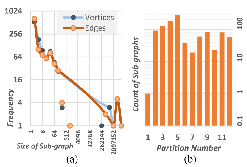
Figure 5: Frequency distribution of (a) # of vertices & edges per sub-graph, and (b) # of sub-graphs per partition. Log scale.

The TR time-series graph collection is partitioned across 12 hosts in a commodity cluster. The partitions have between $1$ and $285$ sub-graph each, with the number of vertices/edge per sub-graph ranging from $1/0$ to $5,803,661/6,511,896$ (Fig. 5). As can be imagined, there is an inverse correlation between the number of sub-graphs in a partition and the sizes of sub-graphs in it. Each host has an 8-core Intel Xeon CPU, 16 GB RAM and 1 TB SATA HDD and is inter-connected by a Gigabit Ethernet. The hosts run 64-bit Java 7 on Ubuntu Linux.

We implement three different applications, that span the three design patterns emphasized in this paper: Single Source Shortest Path (SSSP) (sequentially dependent), N-hop latency (eventually dependent), and PageRank (independent). SSSP finds the shortest path from a source IP address for an instance to all other IP addresses using the A^⋆/Dijkstra’s algorithm, with latency as the edge weight. These distances are incrementally aggregated between instances. N-hop latency builds a histogram of latency times taken to reach IPs that are ’N’ hops from a source IP; we use $N=6$. These histograms are folded into a composite in the merge step. Lastly, PageRank offers a form of network centrality, and is executed on each instance independently by only considering edges that were active in a trace for that instance’s period.

These applications validate the ability to map meaningful time-series graph analytics to our design patterns using the iBSP model. However, in the interests of space, we limit our detailed analysis to SSSP because: (1) it is a popular, well-understood algorithm that is representative of other traversals; and (2) it uses the sequential design pattern which is the most restrictive in terms of concurrency, hence outlying the system’s behavior under constraints. Furthermore, we can compare these results with prior ones for SSSP on a single template graph using a non-iterative sub-graph centric BSP [6].

VI-B Micro-benchmarks on GoFS Data Layout

There are three aspects of GoFS layout optimizations that we investigate here: temporal packing of instances, bin packing of sub-graphs within a partition, and caching. The configuration of the first two have to be decided at deployment time since they impact slice creation, while the cache size can be configured at runtime by the client using GoFS. We use 4 different deployments of the TR time-series graph collection, which combines a temporal packing of either $1$ instance (i1) or $20$ instances (i20) per slice with a sub-graph bin packing with $20$ bins (s20) or $40$ bins (s40) per partition. Note that i1 refers to no temporal instance packing, while we do not consider the case without sub-graph bin packing since the performance degradation is too high. We also run experiments with caching disabled (c0), and caching enabled with $14$ slice slots (c14), where 14 slots are sufficient to fit at least one slice from each of the 14 attributes available for vertices and edges.

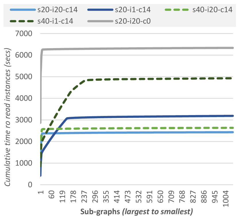
Figure 6: Cumulative time of the total time to read all instances of each sub-graph. X Axis shows incremental sub-graphs being added, largest to smallest.

As a high level comparison, for each of the deployments, we scan through all the sub-graphs, and for each, we load all their instances. This translates to about 152,000 sub-graph instances read. We then sum the total read time for all instances for each sub-graph, and plot this total read time cumulatively for all the sub-graphs. Fig. 6 shows this, with the sub-graphs on the X axis sorted from largest to smallest. So $X=1$ identifies the time to read all 146 instances of the largest sub-graph, while $X=1044$ is the total time to read all instances of all 1044 sub-graphs across the 12 partitions. We plot the cached version for all deployments, and one non-cached version is shown.

The plot illustrates the overall benefits of temporal packing, when we compare s20-i20-c14 and s20-i1-c14 (light and dark blue solid lines), and s40-i20-c14 and s40-i1-c14 (light and dark green dotted lines). For large sub-graphs on the left, the size of just a single sub-graph instance on disk is large, and even without temporal packing (i=1), the disk latency cost is amortized over the loading time of the large, single-instance slice. With packing (i=20), we actually see poorer performance for large sub-graphs since the slice size is much larger for 20 instances and there may be file fragmentation and memory pressure effects. However, as we include more modest sized sub-graphs, the benefits of temporal packing starts to be exhibited. The cross over point is about 80 sub-graphs, for s20, beyond which temporal packing outperforms non-packing.

Similarly, for sub-graph bin packing, using 20 bins shows a marked benefit over 40 bins, with the benefits being larger when temporal packing is not used. This is understandable since not using temporal packing and using a large number of bins causes slice sizes to be smaller and the disk latency to dominate. With temporal packing, there is a tangible but smaller difference between bin sizes of 20 and 40. As the bin size increases, and tends towards the number of sub-graphs in the partition, this degenerates to non-bin packing approach.

The impact of caching is apparent in the single gray solid line at the top shown for s20-i20-c0. It is almost three time as large as the cached version for s20-i20-c14. Hence, the benefits of temporal packing and sub-graph binning are reaped only when combined with caching, as otherwise, they fail to leverage the pre-fetching benefits of locality end up I/O bound.

VI-C Application Benchmark of SSSP

We evaluate the iBSP implementation of temporal traversal of SSSP over multiple instances using a sequentially dependent pattern. The iBSP SSSP is run on three different configurations of the TR time-series graph, s20-i20-c0, s20-i1-c14 and s20-i20-c14, which are respectively temporal packing of 20 without caching, no temporal packing with caching, and temporal packing and caching enabled, all with sub-graph binning enabled with 20 bins.

Fig. 7 studies the time taken per timestep iteration, each corresponding to an SSSP on one graph instance. The Y axis shows the total time taken by one BSP while the X axis show sequentially increasing instances, with the first 11 being shown for conciseness. The bars in each cluster refer to a different configuration of GoFS. We can see that the first timestep dominates, and this is because the graph template is loaded as part of this timestep. Note that the template is loaded just once at the start of the iBSP application. As we progress along the second and subsequent timesteps, we see modest differences in the timings for each timestep for different GoFS configurations. The penalty for not caching is evident in the first bar for s20-i20-c0, while the distinction between enabling temporal packing or not, in the second and third bars, is less obvious. The domination of compute time for SSSP hides the differences, which also means that the application is more compute bound than I/O bound, as we prefer.

Fig. 8 offers a different view for this same experiment, from the perspective of the cumulative number of slices that are read from disk as the timesteps progress. Here, the lack of caching shows the high slope for the solid light blue line for s20-i20-c0, while we see a tangible difference in the number of slices read with and without temporal packing.

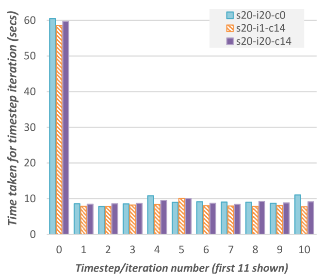
Figure 7: Time per iteration (secs) for first 11 iterations of the iBSP SSSP application are shown for two deployments and cache sizes. Timestep 0 includes template load time.

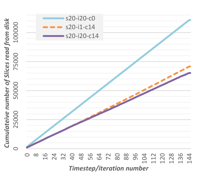
Figure 8: Cumulative number of slices loaded (Y axis) for different deployments and caching, as the timesteps progress along X Axis for the iBSP SSSP application.

VII Conclusions

In summary, we have introduced and formalized the notion of time-series graph models as a first class Big Data constituent that is of growing importance. We propose several design patterns for composing analytics on top of this data model, and define an iterative BSP abstraction to define such patterns for distributed execution. This leverages our existing work on sub-graph centric programming for single graphs, and offers a high degree of parallelism, in space and in time. This concurrency is made use of by Gopher which executes iBSP on commodity clusters, on conjunction with the GoFS distributed graph data store, which is optimized for time-series graphs and the proposed design patterns. The benefits of these are empirically validated for several GoFS configurations for a canonical iterative SSSP application. These form a compelling basis for further investigation into this novel Big Data and distributed abstractions space, with additional optimization problems open to leverage the degrees of parallelism that we have exposed.

References

- [1] L. Atzori, A. Iera, and G. Morabito, “The internet of things: A survey,” Computer Networks, vol. 54, no. 15, 2010.
- [2] V. Kostakos, “Temporal graphs,” Physica A, vol. 388, no. 6, 2009.
- [3] R. Cheng, J. Hong, A. Kyrola, Y. Miao, X. Weng, M. Wu, F. Yang, L. Zhou, F. Zhao, and E. Chen, “Kineograph: taking the pulse of a fast-changing and connected world,” in EuroSys, 2012.
- [4] C. Cortes, D. Pregibon, and C. Volinsky, “Computational methods for dynamic graphs,” AT&T Shannon Labs, Tech. Rep., 2004.
- [5] H. Tong, S. Papadimitriou, P. S. Yu, and C. Faloutsos, “Proximity tracking on time-evolving bipartite graphs,” in SDM, 2008.
- [6] Y. Simmhan, A. Kumbhare, C. Wickramaarachchi, S. Nagarkar, S. Ravi, C. Raghavendra, and V. Prasanna, “Goffish: A sub-graph centric framework for large-scale graph analytics,” arXiv, Tech. Rep. 1311.5949, 2013, under review.
- [7] L. G. Valiant, “A bridging model for parallel computation,” CACM, vol. 33, no. 8, 1990.
- [8] G. Malewicz, M. H. Austern, A. J. Bik, J. C. Dehnert, I. Horn, N. Leiser, and G. Czajkowski, “Pregel: A system for large-scale graph processing,” in SIGMOD, 2010.
- [9] C. Avery, “Giraph: Large-scale graph processing infrastructure on hadoop,” in Hadoop Summit, 2011.
- [10] S. Salihoglu and J. Widom, “GPS: A Graph Processing System,” in SSDBM, 2013.
- [11] J. Dean and S. Ghemawat, “Mapreduce: simplified data processing on large clusters,” CACM, vol. 51, no. 1, 2008.
- [12] U. Kang, C. E. Tsourakakis, A. P. Appel, C. Faloutsos, and J. Leskovec, “Hadi: Mining radii of large graphs,” TKDD, vol. 5, 2011.
- [13] J. Cohen, “Graph twiddling in a mapreduce,” CiSE, vol. 11, no. 4, 2009.
- [14] J. Ekanayake, H. Li, B. Zhang, T. Gunarathne, S.-H. Bae, J. Qiu, and G. Fox, “Twister: a runtime for iterative mapreduce,” in HPDC, 2010.
- [15] R. Pike, S. Dorward, R. Griesemer, and S. Quinlan, “Interpreting the data: Parallel analysis with sawzall,” Scientific Programming, vol. 13, no. 4, 2005.
- [16] A. Lumsdaine, D. Gregor, B. Hendrickson, and J. Berry, “Challenges in parallel graph processing,” Parallel Processing Letters, vol. 17, no. 01, pp. 5–20, 2007.
- [17] M. Redekopp, Y. Simmhan, and V. Prasanna, “Optimizations and analysis of bsp graph processing models on public clouds,” in IPDPS, 2013.
- [18] Y. Low, D. Bickson, J. Gonzalez, C. Guestrin, A. Kyrola, and J. M. Hellerstein, “Distributed graphlab: A framework for machine learning and data mining in the cloud,” VLDB, vol. 5, no. 8, 2012.
- [19] B. Shao, H. Wang, and Y. Li, “Trinity: A distributed graph engine on a memory cloud,” in SIGMOD, 2013.