The geometric Cauchy problem for
the membrane shape equation

Abstract.

We address the geometric Cauchy problem for surfaces associated to the membrane shape equation describing equilibrium configurations of vesicles formed by lipid bilayers. This is the Euler–Lagrange equation of the Canham–Helfrich–Evans elastic curvature energy subject to constraints on the enclosed volume and the surface area. Our approach uses the method of moving frames and techniques from the theory of exterior differential systems.

1. Introduction

Lipid bilayers are the basic elements of biological membranes and constitute the main separating structure of living cells. In aqueous solution, lipid bilayers typically form closed surfaces or vesicles (closed bilayer films) which exhibit a large variety of different shapes, such as the non-spherical, biconcave shape characteristic of red blood cells [13, 22, 36]. Since in most biologically significant cases the width of the membrane exceeds the thickness by several orders of magnitude, the membrane can be regarded as a two-dimensional surface $S$ embedded in three-dimensional space $\mathbb{R}^{3}$, with enclosed volume $V(S)$ and surface area $A(S)$.

A continuum-mechanical description of lipid bilayers which has been shown to be predictive with respect to the observed shapes dates from the work of Canham [10], Helfrich [19], and Evans [14] at the beginning of the 1970s. In the Canham–Helfrich–Evans model, an equilibrium configuration $S$, at fixed volume and surface area, is determined by minimization of the elastic bending energy [19, 20, 31, 34, 35, 37, 38, 41, 42]

(1.1) $$\mathcal{F}(S)=\frac{k}{2}\int_{S}{(2H+c_{0})^{2}dA}+\bar{k}\int_{S}{KdA}+p{V(S)}+\lambda{A(S)}.$$

Here $H=(a+c)/2$ and $K=ac$ are the mean and Gauss curvatures of the surface $S$, where $a$ and $c$ denote the principal curvatures, $dA$ is the area element, and $k$, $\bar{k}$, $c_{0}$, $p$, and $\lambda$ are constants: $k$, $\bar{k}$ are material dependent elasticity parameters, $c_{0}$ is the spontaneous curvature, $p$ denotes the difference between the outside and the inside pressure, and $\lambda$ is the surface lateral tension. The pressure $p$ and the tension $\lambda$ play the role of Lagrange multipliers for the constraints of constant volume and surface area.

The Euler–Lagrange equation of the functional (1.1), often referred to as the membrane shape equation or the Ou-Yang–Helfrich equation, takes the form [32, 33]

(1.2) $$2k\left\{\Delta H+2H(H^{2}-K)\right\}-\left(2\lambda+kc_{0}^{2}\right)H-2kc_{0}K+p=0,$$

where $\Delta$ denotes the Laplace–Beltrami operator of the induced metric on $S$. This implies that an equilibrium shape surface $S$ satisfies a fourth order nonlinear partial differential equation of the form

(1.3) $$\Delta H=\Phi(a,c),$$

where $\Phi$ is a real analytic symmetric function of the principal curvatures $a$, $c$. Examples of surfaces associated to (1.2) include Willmore surfaces [4, 7, 39, 44], which are solutions of the differential equation

(1.4) $$\Delta H+2H(H^{2}-K)=0.$$

Willmore surfaces are best known in connection to the celebrated Willmore conjecture, recently confirmed by Marques and Neves [23].

The aim of the present paper is to solve the geometric Cauchy problem for the class of surfaces in $\mathbb{R}^{3}$ satisfying the membrane shape equation. More precisely, we shall prove the following.

Theorem 1.

Let $\alpha:J\to\mathbb{R}^{3}$ be a real analytic curve with $\|\alpha^{\prime}(x)\|=1$, where $J\subset\mathbb{R}$ is an open interval. Let $(T=\alpha^{\prime}$, $N$, $B)$ be the Frenet frame field along $\alpha$, with Frenet–Serret equations

$$T^{\prime}=\kappa N,\quad N^{\prime}=-\kappa T+\tau B,\quad B^{\prime}=-\tau N,$$

where $\kappa(x)\neq 0$ is the curvature and $\tau(x)$ is the torsion of $\alpha$. For $x_{0}\in J$, consider the unit normal vector $W_{0}=N(x_{0})\cos{a_{0}}+B(x_{0})\sin{a_{0}}$. Let $h$, $h^{W}:J\to\mathbb{R}$ be two real analytic functions and assume that

(1.5) $$h+\kappa\sin{\left(-\int_{x_{0}}^{x}\tau(u)du+a_{0}\right)}<0.$$

Then, there exists a real analytic immersion $f:\Sigma\to\mathbb{R}^{3}$, where $\Sigma\subset\mathbb{R}^{2}$ is an open neighborhood of $J\times\{0\}$, with principal curvature line coordinates $(x,y)$, such that:

1. the mean curvature $H$ of $f$ satisfies

   $$\Delta H=\Phi(a,c);$$

2. the restriction $f|_{J}=\alpha$;

3. the tangent plane to $f$ at $f(x_{0},0)$ is spanned by $T(x_{0})$ and $W_{0}$;

4. $\alpha$ is a curvature line of $f$;

5. $H|_{J}=h$ and ${\frac{\partial H}{\partial y}}\big{|}_{J}=h^{W}$.

Moreover, if $\hat{f}:\hat{\Sigma}\to\mathbb{R}^{3}$ is any other principal immersion satisfying the above conditions, then $f(\Sigma\cap\hat{\Sigma})=\hat{f}(\Sigma\cap\hat{\Sigma})$.

The Cauchy problem addressed in Theorem 1 can be viewed as a generalization of similar problems for constant mean curvature surfaces in $\mathbb{R}^{3}$ and for constant mean curvature one surfaces in hyperbolic 3-space [5, 15], which in turn are both inspired by the classical Björling problem for minimal surfaces in $\mathbb{R}^{3}$ [30]. Recently, the geometric Cauchy problem has been investigated for several surface classes and in different geometric situations (see, for instance, [1, 2, 6] and the references therein). However, our approach to the problem is different in that we use techniques from the Cartan–Kähler theory of Pfaffian differential systems and the method of moving frames (see [25] and [26, 27, 28] for a similar approach to the integrable system of Lie-minimal surfaces and other systems in submanifold geometry). This work was mainly motivated by a paper of Tu and Ou-Yang [41], in which the authors propose a geometric scheme to discuss the questions of the shape and stabilities of biomembranes within the framework of exterior differential forms. The first step in our discussion consists in the construction of a Pfaffian differential system (PDS) whose integral manifolds are canonical lifts of principal frames along surfaces satisfying the membrane shape equation (1.3). We then compute the algebraic generators of degree two for such a PDS and show that the polar space of a 1-dimensional integral element is 2-dimensional. Next, by the Cartan–Kähler theorem we deduce the existence of a unique real analytic integral surface passing through a real analytic integral curve. Finally, we build 1-dimensional integral curves from arbitrary real analytic space curves and two real analytic functions. The proof of Theorem 1 follows from a suitable geometric interpretation of these results. Interestingly enough, in the proof of Theorem 1, a crucial role is played by the use of a relatively parallel adapted frame of Bishop [3] along the given curve $\alpha$.

The paper is organized as follows. Section 2 introduces some background material and recalls the basic facts about Pfaffian differential systems in two independent variables. Section 3 constructs the PDS for the class of surfaces associated to the membrane shape equation. Section 4 proves that this PDS is in involution. Section 5 proves Theorem 1. Finally, Section 6 discusses some examples.

For the subject of exterior differential systems we refer the reader to the monographs [8, 12, 17, 18, 21]. The summation convention over repeated indices is used throughout the paper.

The authors would like to thank the referees for their useful comments and suggestions.

2. Background material

2.1. The Euclidean group and the structure equations

Let $\mathbb{E}(3)=\mathbb{R}^{3}\rtimes\mathrm{SO}(3)$ be the Euclidean group of proper rigid motions of $\mathbb{R}^{3}$. A group element of $\mathbb{E}(3)$ is an ordered pair $(P,A)$, where $P\in\mathbb{R}^{3}$ and $A$ is a $3\times 3$ orthogonal matrix with determinant one. If we let $A_{j}\in\mathbb{R}^{3}$, $j=1,2,3$, denote the $j$-th column vector of $A$ and regard $P$ and the $A_{j}$ as $\mathbb{R}^{3}$ valued functions on $\mathbb{E}(3)$, there exist unique left invariant 1-forms $\theta^{i}$ and $\theta^{i}_{j}$, $i,j=1,2,3$, such that

(2.1) $$dP=\theta^{i}A_{i},\quad dA_{j}=\theta^{i}_{j}A_{i},\quad j=1,2,3.$$

The 1-forms $\theta^{i}$, $\theta^{i}_{j}$ are the Maurer–Cartan forms of $\mathbb{E}(3)$. Differentiating the orthogonality condition $A_{i}\cdot A_{j}=\delta_{ij}$ yields $\theta^{i}_{j}=-\theta^{j}_{i}$, $i,j=1,2,3$. These are the only relations among the Maurer–Cartan forms and then $(\theta^{1},\theta^{2},\theta^{3},\theta^{2}_{1},\theta^{3}_{1},\theta^{3}_{2})$ is a basis for the space of left invariant 1-forms on $\mathbb{E}(3)$. Differentiating (2.1), we obtain the structure equations of $\mathbb{E}(3)$

(2.2) $$\begin{cases}d\theta^{1}=\theta^{2}_{1}\wedge\theta^{2}+\theta^{3}_{1}\wedge\theta^{3},\\ d\theta^{2}=-\theta^{2}_{1}\wedge\theta^{1}+\theta^{3}_{2}\wedge\theta^{3},\\ d\theta^{3}=-\theta^{3}_{1}\wedge\theta^{1}-\theta^{3}_{2}\wedge\theta^{2},\end{cases}$$

and

(2.3) $$\begin{cases}d\theta^{2}_{1}=\theta^{3}_{2}\wedge\theta^{3}_{1},\\ d\theta^{3}_{1}=-\theta^{3}_{2}\wedge\theta^{2}_{1},\\ d\theta^{3}_{2}=\theta^{3}_{1}\wedge\theta^{2}_{1}.\end{cases}$$

2.2. Principal frames and invariants

Let $f:X\to\mathbb{R}^{3}$ be a smooth immersion of a connected, orientable 2-dimensional manifold $X$, with unit normal vector field $n$. Consider the orientation of $X$ induced by $n$ from the orientation of $\mathbb{R}^{3}$. Suppose that $f$ is free of umbilic points and with the given normal vector such that the principal curvatures $a$ and $c$ satisfy $a>c$. A principal frame field along $f$ is a map $(f,A):U\to\mathbb{E}(3)$ defined on some open connected set $U\subset X$, such that, for each $\zeta\in U$, the tangent space $df(T_{\zeta}X)=\text{span}\{{A_{1}}(\zeta),A_{2}(\zeta)\}$, $A_{3}(\zeta)=n(\zeta)$, and ${A_{1}}(\zeta)$, $A_{2}(\zeta)$ are along the principal directions corresponding to $a(\zeta)$ and $c(\zeta)$, respectively. Any other principal frame field on $U$ is of the form $(f,(\pm A_{1},\pm A_{2},A_{3}))$. Thus, if $X$ is simply connected, possibly passing to a double cover, we may assume the existence of a globally defined principal frame field $(f,A)$ along $f$. Following the usual practice in the method of moving frames we use the same notation to denote the forms on $\mathbb{E}(3)$ and their pullbacks via $(f,A)$ on $X$.

Let $(f,A)$ be a globally defined principal frame field along $f$. Then on $X$, $(\theta^{1},\theta^{2})$ defines a coframe field, $\theta^{3}$ vanishes identically, and

$$\theta^{3}_{1}=a\theta^{1},\quad\theta^{3}_{2}=c\theta^{2},\quad\theta^{2}_{1}=p\theta^{1}+q\theta^{2},$$

where $a>c$ are the principal curvatures and $p,q$ are smooth functions, the Christoffel symbols of $f$ with respect to $(\theta^{1},\theta^{2})$. The structure equations of $\mathbb{E}(3)$ give

(2.4) $$d\theta^{1}=p\theta^{1}\wedge\theta^{2},\quad d\theta^{2}=q\theta^{1}\wedge\theta^{2},$$

the Gauss equation

(2.5) $$dp\wedge\theta^{1}+dq\wedge\theta^{2}+(ac+p^{2}+q^{2})\theta^{1}\wedge\theta^{2}=0,$$

and the Codazzi equations

(2.6) $$\begin{cases}da\wedge\theta^{1}+p(c-a)\theta^{2}\wedge\theta^{1}=0,\\ dc\wedge\theta^{2}+q(c-a)\theta^{1}\wedge\theta^{2}=0.\end{cases}$$

With respect to the principal frame field $(f,A)$, the first and second fundamental forms of $f$ are given by

$$I=df\cdot df=\theta^{1}\theta^{1}+\theta^{2}\theta^{2},\quad II=-df\cdot dn=a\theta^{1}\theta^{1}+c\theta^{2}\theta^{2}.$$

For any smooth function $g:X\to\mathbb{R}$, we set

(2.7) $$dg=g_{1}\theta^{1}+g_{2}\theta^{2},$$

where the functions $g_{1},g_{2}:X\to\mathbb{R}$ play the role of partial derivatives relative to $\theta^{1},\theta^{2}$. In general, mixed partials are not equal, but satisfy

(2.8) $$g_{12}-g_{21}=pg_{1}+qg_{2},$$

by (2.4). Using the relation

$$(\Delta g)\,\theta^{1}\wedge\theta^{2}=d\ast dg=d(-g_{2}\theta^{1}+g_{1}\theta^{2}),$$

which defines the Laplace–Beltrami operator $\Delta$ of the metric $I$ on $X$, we find

$$\Delta g=g_{11}+g_{22}+qg_{1}-pg_{2}.$$

In this formalism, the Gauss and Codazzi equations can be written as

(2.9) $$\begin{cases}p_{2}-q_{1}=ac+p^{2}+q^{2},\\ a_{2}=-p(c-a),\\ c_{1}=-q(c-a).\end{cases}$$

From this we see that there exists a smooth function $r$, such that

(2.10) $$\begin{cases}p_{2}=r+\frac{1}{2}(ac+p^{2}+q^{2}),\\ q_{1}=r-\frac{1}{2}(ac+p^{2}+q^{2}).\end{cases}$$

Differentiating the structure equations (2.9) and using (2.7) and (2.8), we get

(2.11) $$\begin{cases}a_{21}=(p_{1}-pq)(a-c)+pa_{1},\quad a_{12}=2pa_{1}+p_{1}(a-c),\\ a_{22}=\left(r+\frac{1}{2}(ac+p^{2}+q^{2})\right)(a-c)+p^{2}(a-c)-pc_{2},\\ c_{21}=q_{2}(a-c)-2qc_{2},\quad c_{12}=(q_{2}+pq)(a-c)-qc_{2},\\ c_{11}=\left(r-\frac{1}{2}(ac+p^{2}+q^{2})\right)(a-c)+qa_{1}-q^{2}(a-c).\\ \end{cases}$$

Applying these formulae, we are now able to express the Laplace–Beltrami operator of the mean curvature of the immersion $f$ in terms of the functions $p,q,a,c,r,a_{1},c_{2}$,

(2.12) $$\Delta H=\frac{1}{2}\left(a_{11}+c_{22}\right)-r(c-a)+qa_{1}-pc_{2}.$$

Thus, $f$ satisfies the differential relation $\Delta H=\Phi(a,c)$ if and only if

(2.13) $$a_{11}+c_{22}=2\left(\Psi(p,q,a,c,a_{1},c_{2})+r(c-a)\right)$$

where

$$\Psi(p,q,a,c,a_{1},c_{2})=\Phi(a,c)+pc_{2}-qa_{1}.$$

2.3. Pfaffian differential systems in two independent variables

In this section we recall some basic facts about the Cartan–Kähler theory of Pfaffian differential systems in two independent variables. Let $M$ be a smooth manifold and let

$$\left(\omega^{1},\omega^{2},\eta^{1},\dots,\eta^{k},\pi^{1},\dots,\pi^{s}\right)$$

be a coframe field on $M$. Consider the 2-form $\Omega=\omega^{1}\wedge\omega^{2}$, which is referred to as the independence condition, and let

$$\mathcal{I}=\{\eta^{1},\dots,\eta^{k},d\eta^{1},\dots,d\eta^{k}\}$$

be the ideal of the algebra of exterior differential forms on $M$ generated by the 1-forms $\eta^{1},\dots,\eta^{k}$ and the 2-forms $d\eta^{1},\dots,d\eta^{k}$. The pair $(\mathcal{I},\Omega)$ is called a Pfaffian differential system in two independent variables. A 2-dimensional integral manifold (integral surface) of $(\mathcal{I},\Omega)$ is an immersed 2-dimensional manifold $X\subset M$, not necessarily embedded, such that

$$\Omega|_{X}\neq 0,\quad\eta^{j}|_{X}=d\eta^{j}|_{X}=0,\quad j=1,\dots,k.$$

Similarly, a 1-dimensional integral manifold (integral curve) of the Pfaffian system $(\mathcal{I},\Omega)$ is an immersed 1-dimensional manifold $\mathcal{A}\subset M$, such that

$$\omega^{1}\omega^{1}+\omega^{2}\omega^{2}|_{\mathcal{A}}\neq 0,\quad\eta^{j}|_{\mathcal{A}}=0,\quad j=1,\dots,k.$$

A 1-dimensional integral element of $(\mathcal{I},\Omega)$, at a fixed point $m\in M$, is a 1-dimensional subspace $[\xi]$ of $T_{m}M$, spanned by a non-zero tangent vector $\xi$, such that

$$\omega^{1}(\xi)\omega^{1}(\xi)+\omega^{2}(\xi)\omega^{2}(\xi)\neq 0,\quad\eta^{j}(\xi)=0,\quad j=1,\dots,k.$$

Similarly, a 2-dimensional integral element of $(\mathcal{I},\Omega)$ is a 2-dimensional subspace $W$ of $T_{m}M$, such that

$$\Omega|_{W}\neq 0,\quad\eta^{j}|_{W}=d\eta^{j}|_{W}=0,\quad j=1,\dots,k.$$

Given a 1-dimensional integral element $[\xi]$, its polar space $H([\xi])$ is the subspace of $T_{m}M$ defined by the linear equations:

$$\eta^{j}=0,\quad i_{\xi}d\eta^{j}=0,\quad j=1,\dots,k.$$

If

(2.14) $$\mathrm{dim\,}H([\xi])=2,\quad\text{and}\quad\Omega|_{H([\xi])}\neq 0,$$

then $H([\xi])$ is the unique 2-dimensional integral element containing $[\xi]$. The following statement is a consequence of the general Cartan–Kähler theorem for exterior differential systems in involution [8, 12].

Theorem 2.

Let $M$ be a real analytic manifold and assume the the coframe field

$$\left(\omega^{1},\omega^{2},\eta^{1},\dots,\eta^{k},\pi^{1},\dots,\pi^{s}\right)$$

is real analytic. If condition (2.14) is satisfied for every 1-dimensional integral element, then for any real analytic 1-dimensional integral curve $\mathcal{A}\subset M$ there exists a 2-dimensional integral manifold $X\subset M$ such that $\mathcal{A}\subset X$. The manifold $X$ is unique, in the sense that if $\tilde{X}$ is another 2-dimensional integral manifold passing through $\mathcal{A}$, then there exists an open neighborhood $U\subset M$ of $\mathcal{A}$ such that $\tilde{X}\cap U=X\cap U$.

3. The Pfaffian differential system of lipid bilayer membranes

3.1. Principal frames

Let $Y_{(1)}$ be the 10-dimensional manifold

$$Y_{(1)}=\mathbb{E}(3)\times\left\{(p,q,a,c)\in\mathbb{R}^{4}\,|\,a-c>0\right\}.$$

Let

$$\theta^{1},\theta^{2},\theta^{3},\theta^{2}_{1},\theta^{3}_{1},\theta^{3}_{2}$$

be the basis of left invariant Maurer–Cartan forms of $\mathbb{E}(3)$ which satisfy structure equations (2.2) and (2.3).

On $Y_{(1)}$ consider the Pfaffian differential system $(\mathcal{I}_{1},\Omega)$ differentially generated by the 1-forms

(3.1) $$\begin{array}[]{ll}\alpha^{1}=\theta^{3},&\alpha^{2}=\theta^{2}_{1}-p\theta^{1}-q\theta^{2},\\ \alpha^{3}=\theta^{3}_{1}-a\theta^{1},&\alpha^{4}=\theta^{3}_{2}-c\theta^{2},\\ \end{array}$$

with independence condition $\Omega=\theta^{1}\wedge\theta^{2}$.

Remark 1.

The integral manifolds of $(\mathcal{I}_{1},\Omega)$ are the second order prolongations of umbilic free immersed surfaces in $\mathbb{R}^{3}$, i.e., smooth maps

$$F_{(1)}:=(F,A,p,q,a,c):X\to Y_{(1)}$$

defined on an oriented, connected 2-dimensional manifold $X$ such that:

• $F:X\to\mathbb{R}^{3}$ is an umbilic free smooth immersion;

• $(F,A)=(F,(A_{1},A_{2},A_{3})):X\to\mathbb{E}(3)$ is a principal frame field along $F$;

• $(\theta^{1},\theta^{2})$ is a positively oriented orthonormal coframe, dual to the trivialization of $dF(T(X))$ defined by the tangent vector fields $A_{1}$, $A_{2}$ along $F$;

• $\theta^{1}\theta^{1}+\theta^{2}\theta^{2}$ is the first fundamental form induced by $F$;

• $A_{1},A_{2}$ are tangent to the principal curvature lines of $F$;

• $\theta^{2}_{1}=p\theta^{1}+q\theta^{2}$ is the Levi Civita connection with respect to $(\theta^{1},\theta^{2})$;

• $a$ and $c$ are the principal curvatures of $F$ and $a>c$;

• $a\theta^{1}\theta^{1}+c\theta^{2}\theta^{2}$ is the second fundamental form of $F$;

• $A_{3}$ is the Gauss map of $F$.

Note that $F_{(1)}$ is uniquely determined by the orientation of $X$, by the umbilic free immersion $F$, and by the assumption that $a>c$.

From the structure equations (2.2) and (2.3), we obtain, modulo the algebraic ideal $\{\alpha^{j}\}$ generated by the 1-forms $\alpha^{1},\dots,\alpha^{4}$,

(3.2) $$\begin{cases}d\theta^{1}\equiv p\theta^{1}\wedge\theta^{2},\\ d\theta^{2}\equiv q\theta^{1}\wedge\theta^{2},\\ \end{cases}\mod\{\alpha^{j}\}$$

and

(3.3) $$\begin{cases}d\alpha^{1}\equiv 0,\\ d\alpha^{2}\equiv-dp\wedge\theta^{1}-dq\wedge\theta^{2}-(ac+p^{2}+q^{2})\theta^{1}\wedge\theta^{2},\\ d\alpha^{3}\equiv-da\wedge\theta^{1}+p(c-a)\theta^{1}\wedge\theta^{2},\\ d\alpha^{4}\equiv-dc\wedge\theta^{2}-q(c-a)\theta^{1}\wedge\theta^{2}.\\ \end{cases}\mod\{\alpha^{j}\}$$

3.2. Prolongation

Let $Y_{(2)}$ be the 17-dimensional manifold

$$Y_{(2)}=Y_{(1)}\times\left\{(p_{1},q_{2},r,a_{1},c_{2},a_{11},c_{22})\in\mathbb{R}^{7}\right\},$$

where

$$(p_{1},q_{2},r,a_{1},c_{2},a_{11},c_{22})$$

are the new fiber coordinates. Consider on $Y_{(2)}$ the Pfaffian differential system $(\mathcal{I}_{2},\Omega)$ differentially generated by the 1-forms

$$(\alpha^{1},\dots,\alpha^{4},\beta^{1},\beta^{2},\gamma^{1},\gamma^{2},\delta^{1},\delta^{2}),$$

where $\alpha^{1},\dots,\alpha^{4}$ are defined as in (3.1) and

(3.4) $$\begin{cases}\beta^{1}=dp-p_{1}\theta^{1}-(r+\frac{1}{2}(ac+p^{2}+q^{2}))\theta^{2},\\ \beta^{2}=dq-(r-\frac{1}{2}(ac+p^{2}+q^{2}))\theta^{1}-q_{2}\theta^{2},\\ \gamma^{1}=da-a_{1}\theta^{1}+p(c-a)\theta^{2},\\ \gamma^{2}=dc+q(c-a)\theta^{1}-c_{2}\theta^{2},\\ \delta^{1}=da_{1}-a_{11}\theta^{1}+(-2a_{1}p+(c-a)p_{1})\theta^{2},\\ \delta^{2}=dc_{2}+(2c_{2}q+(c-a)q_{2})\theta^{1}-c_{22}\theta^{2}.\\ \end{cases}$$

From (3.3) and (3.4) it follows that, modulo the algebraic ideal generated by $\alpha^{j}$, $\beta^{a}$, $\gamma^{a}$ and $\delta^{a}$, $j=1,2,3,4;a=1,2$, we have

(3.5) $$\begin{cases}d\alpha^{j}\equiv 0,\quad j=1,2,3,4,\\ d\gamma^{a}\equiv 0,\quad a=1,2,\\ \end{cases}\mod\{\alpha^{j},\beta^{a},\gamma^{a},\delta^{a}\}$$

Remark 2.

The integral manifolds of $(\mathcal{I}_{2},\Omega)$ are fourth order prolongations of immersed surfaces in $\mathbb{R}^{3}$, that is, smooth maps

$$F_{(2)}:=(F,A,p,q,a,c,p_{1},q_{2},r,a_{1},c_{2},a_{11},c_{22}):X\to Y_{(2)},$$

where $(F,A,p,q,a,c):X\to Y_{(1)}$ is an extended principal frame along $F$ and the functions

$$p_{1},q_{2},r,a_{1},c_{2},a_{11},c_{22}:X\to\mathbb{R}$$

are defined by

$$\begin{cases}dp=p_{1}\theta^{1}+p_{2}\theta^{2},\quad dq=q_{1}\theta^{1}+q_{2}\theta^{2},\\ r=p_{2}-\frac{1}{2}(ac+p^{2}+q^{2})=q_{1}+\frac{1}{2}(ac+p^{2}+q^{2}),\\ da=a_{1}\theta^{1}+a_{2}\theta^{2},\quad dc=c_{1}\theta^{1}+c_{2}\theta^{2},\\ da_{1}=a_{11}\theta^{1}+a_{12}\theta^{2},\quad dc_{2}=c_{21}\theta^{1}+c_{22}\theta^{2}.\end{cases}$$

Note that $F_{(2)}$ is uniquely determined by the orientation of $X$, by the immersion $F$, and by the assumption that the principal curvature satisfy $a>c$.

The canonical prolongations of smooth immersions $F:X\to\mathbb{R}^{3}$ satisfying the partial differential relation

$$\Delta H=\Phi(a,c)$$

are characterized by the equation

(3.6) $$a_{11}+c_{22}=2\left[\Phi(a,c)+r(c-a)-qa_{1}+pc_{2}\right].$$

3.3. The Pfaffian differential system of lipid bilayer membranes

Let $Y_{\ast}$ be the 16-dimensional real analytic submanifold of $Y_{(2)}$ defined by

$$a_{11}+c_{22}=2\left[\Phi(a,c)+r(c-a)-qa_{1}+pc_{2}\right].$$

On $Y_{\ast}$ we consider the fiber coordinates

$$p,q,a,c,p_{1},q_{2},r,a_{1},c_{2},\ell,$$

where $\ell$ is given by

(3.7) $$\begin{cases}a_{11}=\ell+r(c-a)+\Psi(p,q,a,c,a_{1},c_{2}),\\ c_{22}=-\ell+r(c-a)+\Psi(p,q,a,c,a_{1},c_{2}),\\ \end{cases}$$

where

$$\Psi(p,q,a,c,a_{1},c_{2})=\Phi(a,c)-qa_{1}+pc_{2}.$$

Definition 1.

The restriction of $(\mathcal{I}_{2},\Omega)$ to $Y_{\ast}$ is denoted by $(\mathcal{I}_{\ast},\Omega)$ and is referred to as the Pfaffian exterior differential system of lipid bilayer membranes satisfying the differential relation

$$\Delta H=\Phi(a,c).$$

Remark 3.

The integral manifolds of $(\mathcal{I}_{*},\Omega)$ are canonical prolongations of umbilic free immersions $F:X\to\mathbb{R}^{3}$ whose mean curvature $H$ satisfies $\Delta H=\Phi(a,c)$.

4. Involution

4.1. Algebraic generators

By construction, the Pfaffian differential system $\mathcal{I}_{*}$ is generated, as a differential ideal, by the restrictions to $Y_{*}$ of the 1-forms $\alpha^{j}$, $\beta^{a}$, $\gamma^{a}$, $\delta^{a}$, $j=1,\dots,4;a=1,2$. The generators $\alpha^{j},\beta^{a},\gamma^{a}$ are expressed in terms of the fiber coordinates $p,q,a,c,r,a_{1},c_{2},p_{1},q_{2}$ as in (3.1) and (3.4), while the generators $\delta^{1}$ and $\delta^{2}$ are given by

(4.1) $$\begin{cases}\delta^{1}=da_{1}-\left(\ell+r(c-a)+\Psi\right)\theta^{1}+\left(p_{1}(c-a)-2a_{1}p\right)\theta^{2},\\ \delta^{2}=dc_{2}+\left(q_{2}(c-a)+2c_{2}q\right)\theta^{1}+\left(\ell-r(c-a)-\Psi\right)\theta^{2}.\\ \end{cases}$$

Observe that

$$(\theta^{1},\theta^{2},\alpha^{1},\dots\alpha^{4},\beta^{1},\beta^{2},\gamma^{1},\gamma^{2},\delta^{1},\delta^{2},dp_{1},dq_{2},dr,d\ell)$$

is a global coframe field on $Y_{*}$. Let

$$\left({\partial}_{\theta^{1}},{\partial}_{\theta^{2}},{\partial}_{\alpha^{1}},\dots,{\partial}_{\alpha^{4}},{\partial}_{\beta^{1}},{\partial}_{\beta^{2}},{\partial}_{\gamma^{1}},{\partial}_{\gamma^{2}},{\partial}_{\delta^{1}},{\partial}_{\delta^{2}},{\partial}_{dp_{1}},{\partial}_{dq_{2}},{\partial}_{dr},{\partial}_{d\ell}\right)$$

denote its dual basis on $T(Y_{*})$. According to (3.5), we have

(4.2) $$\begin{cases}d\alpha^{j}\equiv 0,\quad j=1,2,3,4,\\ d\gamma^{a}\equiv 0,\quad a=1,2,\\ \end{cases}\mod\{\alpha^{j},\beta^{a},\gamma^{a},\delta^{a}\}.$$

Thus, the differential ideal $\mathcal{I}_{*}$ is algebraically generated by $\alpha^{j}$, $\beta^{a}$, $\gamma^{a}$, $\delta^{a}$, $j=1,2,3,4;a=1,2$, and by the exterior differential 2-forms $d\beta^{a}$, $d\delta^{a}$, $a=1,2$. Using (3.2), (3.4), (4.1) and (4.2), we obtain, modulo the algebraic ideal $\{\alpha^{j},\beta^{a},\gamma^{a},\delta^{a}\}$,

(4.3) $$\begin{cases}d\beta^{1}\equiv-dp_{1}\wedge\theta^{1}-dr\wedge\theta^{2}-B^{1}\theta^{1}\wedge\theta^{2},\\ d\beta^{2}\equiv-dr\wedge\theta^{1}-dq_{2}\wedge\theta^{2}-B^{2}\theta^{1}\wedge\theta^{2},\\ d\delta^{1}\equiv-d\ell\wedge\theta^{1}-(c-a)dr\wedge\theta^{1}+(c-a)dp_{1}\wedge\theta^{2}-D^{1}\theta^{1}\wedge\theta^{2},\\ d\delta^{2}\equiv(c-a)dq_{2}\wedge\theta^{1}+d\ell\wedge\theta^{2}-(c-a)dr\wedge\theta^{2}+D^{2}\theta^{1}\wedge\theta^{2},\\ \end{cases}$$

where $B^{a}$ and $D^{a}$, $a=1,2$, are real analytic functions of the fiber coordinates.

Remark 4.

Note that if $\Psi$ is polynomial, the $B^{a}$ and the $D^{a}$ are polynomial functions of the fiber coordinates. This is still true of the $B^{a}$, but not of the $D^{a}$, in the event that $\Psi$ is not a polynomial.

In conclusion, we have proved that $(\mathcal{I}_{*},\Omega)$ is algebraically generated by $\alpha^{j}$, $\beta^{a}$, $\gamma^{a}$, $\delta^{a}$ and by

(4.4) $$\begin{cases}\Omega^{1}=dp_{1}\wedge\theta^{1}+dr\wedge\theta^{2}+B^{1}\theta^{1}\wedge\theta^{2},\\ \Omega^{2}=dr\wedge\theta^{1}+dq_{2}\wedge\theta^{2}+B^{2}\theta^{1}\wedge\theta^{2},\\ \Omega^{3}=d\ell\wedge\theta^{1}+(c-a)dr\wedge\theta^{1}-(c-a)dp_{1}\wedge\theta^{2}+D^{1}\theta^{1}\wedge\theta^{2},\\ \Omega^{4}=(c-a)dq_{2}\wedge\theta^{1}+d\ell\wedge\theta^{2}-(c-a)dr\wedge\theta^{2}+D^{2}\theta^{1}\wedge\theta^{2}.\\ \end{cases}$$

4.2. Polar equations

Let $[\xi]$ be a 1-dimensional integral element, where $\xi\in T_{m}Y_{*}$ is a tangent vector of the form

$$\xi=x^{1}{\partial}_{\theta^{1}}+x^{2}{\partial}_{\theta^{2}}+x^{3}{\partial}_{dp_{1}}+x^{4}{\partial}_{dq_{2}}+x^{5}{\partial}_{dr}+x^{6}{\partial}_{d\ell},\quad(x^{1})^{2}+(x^{2})^{2}\neq 0.$$

Its polar space $H([\xi])$ is the subspace tangent to $Y_{*}$ defined by the polar equations

$$\alpha^{j}=0,\quad\beta^{a}=0,\quad\gamma^{a}=0,\quad\delta^{a}=0,\quad i_{\xi}\Omega^{j}=0,\quad j=1,\dots,4;a=1,2.$$

From (4.4), it follows that the polar equations are linearly independent provided $c-a\neq 0$, for every 1-dimensional integral element $[\xi]$. This implies that $H([\xi])$ is the unique 2-dimensional integral element containing $[\xi]$. Thus, by the Cartan–Kähler theorem we have the following.

Theorem 3.

The Pfaffian differential system $(\mathcal{I}_{*},\Omega)$ is in involution and its general solutions depend on four functions in one variable. More precisely, for every, 1-dimensional real analytic integral manifold $\mathcal{A}\subset Y_{*}$ there exists a real analytic 2-dimensional integral manifold $\mathcal{X}\subset Y_{*}$ passing through $\mathcal{A}$. In addition, the 1-dimensional integral manifolds depend on four functions in one variable.

Remark 5.

Note that the functional dependence of the general solutions agrees with that of the initial data of Theorem 1. In fact, besides constants, specifying the initial data of Theorem 1 amounts to the choice of a unit-speed curve $\alpha$ in $\mathbb{R}^{3}$, which depends on two arbitrary functions in one variable, and two functions $h$, $h^{W}$.

Remark 6.

The 2-dimensional integral manifold $\mathcal{X}$ passing through $\mathcal{A}$ is unique, in the sense that if $\tilde{\mathcal{X}}\subset Y_{*}$ is another real analytic 2-dimensional integral manifold containing $\mathcal{A}$, then $\mathcal{X}$ and $\tilde{\mathcal{X}}$ agree in a neighborhood of $\mathcal{A}$.

5. The proof of Theorem 1

We are now ready to prove Theorem 1. We are given the Cauchy data $\alpha$, $x_{0}$, $W_{0}$, $h$, $h^{W}$, consisting of a real analytic curve $\alpha:J\to\mathbb{R}^{3}$, a point $x_{0}\in J$, a unit normal vector $W_{0}=\cos a_{0}N(x_{0})+\sin a_{0}B(x_{0})$, and two real analytic functions $h$, $h^{W}:J\to\mathbb{R}^{3}$ as in the statement of Theorem 1. Set

$$s(x)=-\int_{x_{0}}^{x}{\tau(u)du+a_{0}},$$

so that $s:J\to\mathbb{R}$ is real analytic and $s(x_{0})=a_{0}$, and define

$$m:=-h-\kappa\sin s(x)>0.$$

Let $W:J\to\mathbb{R}^{3}$ be the unit normal vector field along $\alpha$ defined by

$$W=\cos s(x)N+\sin s(x)B.$$

Consider the positively oriented orthonormal frame field given by

(5.1) $$\mathcal{G}=(\alpha,T,W,\text{\sc J}W):J\to\mathbb{E}(3),$$

where

$$\text{\sc J}W=-\sin s(x)N+\cos s(x)B.$$

Using the Frenet–Serret equations $T^{\prime}=\kappa N$, $N^{\prime}=-kT+\tau B$, $B^{\prime}=-\tau N$ for the Frenet frame $(T,N,B)$, it is easily seen that

$$\frac{d\mathcal{G}}{dx}=\mathcal{G}\begin{pmatrix}0&0&0&0\\ 1&0&-\mathfrak{p}&-\mathfrak{a}\\ 0&\mathfrak{p}&0&0\\ 0&\mathfrak{a}&0&0\\ \end{pmatrix},$$

where $\mathfrak{p}$, $\mathfrak{a}:J\to\mathbb{R}$ are the real analytic functions

$$\mathfrak{p}=\kappa\cos s(x),\quad\mathfrak{a}=-\kappa\sin s(x).$$

Remark 7.

The frame field $(T,W,\text{\sc J}W)$ is a relatively parallel adapted frame along the curve $\alpha$ in the sense of Bishop [3].

Next, if we set

(5.2) $$\begin{cases}\mathfrak{c}=\mathfrak{a}-2m,\\ \mathfrak{q}=-\frac{1}{\mathfrak{c}-\mathfrak{a}}\frac{d\mathfrak{c}}{dx},\\ {\mathfrak{a}}_{1}=\frac{d\mathfrak{a}}{dx},\\ {\mathfrak{c}}_{2}=2h^{W}+\mathfrak{p}(\mathfrak{c}-\mathfrak{a}),\\ {\mathfrak{p}}_{1}=\frac{d\mathfrak{p}}{dx},\\ {\mathfrak{q}}_{2}=-\frac{1}{\mathfrak{c}-\mathfrak{a}}\left(\frac{d{\mathfrak{c}}_{2}}{dx}+2{\mathfrak{c}}_{2}\mathfrak{q}\right),\\ \mathfrak{r}=\frac{d{\mathfrak{q}}}{dx}+\frac{1}{2}(\mathfrak{a}\mathfrak{c}+\mathfrak{p}^{2}+\mathfrak{q}^{2}),\\ \mathfrak{l}=\frac{d^{2}{\mathfrak{a}}}{dx^{2}}-\mathfrak{r}(\mathfrak{c}-\mathfrak{a})-\Psi(\mathfrak{p},\mathfrak{q},{\mathfrak{a}}_{1},{\mathfrak{c}}_{2}),\end{cases}$$

then

(5.3) $$\mathcal{A}:J\to Y_{*},\,x\mapsto\left(\mathcal{G},\mathfrak{p},\mathfrak{q},\mathfrak{a},\mathfrak{c},{\mathfrak{p}}_{1},{\mathfrak{q}}_{2},\mathfrak{r},{\mathfrak{a}}_{1},{\mathfrak{c}}_{2},\mathfrak{l}\right)|_{x}$$

is a 1-dimensional integral manifold of $\mathcal{I}_{*}$ such that

$$\theta^{1}=dx,\quad\theta^{2}=0,$$

defined by

(5.4) $$\begin{cases}p\circ\mathcal{A}=\mathfrak{p},\quad q\circ\mathcal{A}=\mathfrak{q},\\ a\circ\mathcal{A}=\mathfrak{a},\quad c\circ\mathcal{A}=\mathfrak{c},\\ p_{1}\circ\mathcal{A}={\mathfrak{p}}_{1},\quad q_{2}\circ\mathcal{A}={\mathfrak{q}}_{2},\\ r\circ\mathcal{A}=\mathfrak{r},\\ a_{1}\circ\mathcal{A}={\mathfrak{a}}_{1},\quad c_{2}\circ\mathcal{A}={\mathfrak{c}}_{2},\\ l\circ\mathcal{A}=\mathfrak{l}.\end{cases}$$

Definition 2.

We call $\mathfrak{U}:=\text{Im}\,\mathcal{A}\subset Y_{*}$ the canonical 1-dimensional integral manifold defined by the Cauchy data $\left(\alpha,x_{0},W_{0},h,h^{W}\right)$.

For a set of Cauchy data $\left(\alpha,x_{0},W_{0},h,h^{W}\right)$, Theorem 3 and Remark 6 imply that there exists a unique real analytic integral manifold $\mathcal{X}\subset Y_{*}$ of $(\mathcal{I}_{*},\Omega)$ such that $\mathfrak{U}\subset\mathcal{X}$, where $\mathfrak{U}$ is the integral curve defined by $\left(\alpha,x_{0},W_{0},h,h^{W}\right)$. On $\mathcal{X}$ we consider the orientation defined by the 2-form $\Omega=\theta^{1}\wedge\theta^{2}$. The map

$$F:\mathcal{X}\ni(P,A,p,q,a,c,p_{1},q_{2},r,a_{1},c_{2},\ell)\mapsto P\in\mathbb{R}^{3}$$

is a real analytic immersion and, by construction, its prolongation $F_{(2)}$ coincides with the inclusion map $\iota:\mathcal{X}\to Y_{*}$. According to Remarks 1 and 2, we infer that

• $\mathcal{X}\ni(P,A,p,q,a,c,p_{1},q_{2},r,a_{1},c_{2},\ell)\mapsto(P,A)\in\mathbb{E}(3)$ is a principal frame field along $F$;

• $F$ satisfies $\Delta H=\Phi(a,c)$;

• $(\theta^{1},\theta^{2})$ is a positively oriented orthonormal principal coframe on $\mathcal{X}$ along the immersion $F$;

• $a,c:\mathcal{X}\to\mathbb{R}$ are the principal curvatures of $F$ and

  $$dH=\frac{1}{2}(da+dc)=\frac{1}{2}(a_{1}-q(c-a))\theta^{1}+\frac{1}{2}(c_{2}-p(c-a))\theta^{2}.$$

Since $\mathcal{X}$ satisfies the initial condition $\mathfrak{U}\subset\mathcal{X}$ and $\mathcal{A}^{*}(\theta^{2})=0$, we can state the following.

Lemma 4.

$\mathcal{A}:J\to\mathcal{X}$ is a curvature line of $F$ such that

$$F\circ\mathcal{A}=\alpha,\quad A\circ\mathcal{A}=\mathcal{G}.$$

In particular, we have

$$F_{*}(T_{\mathcal{A}(x_{0})}(\mathcal{X})=\text{span}\,(A_{1}(\alpha(x_{0})),A_{2}(\alpha(x_{0}))=\text{span}\,(T(x_{0}),W(x_{0})).$$

From (3.4), (5.3) and (5.4), we obtain

(5.5) $$H\circ\mathcal{A}=\frac{1}{2}(\mathfrak{a}+\mathfrak{c})=h$$

and

(5.6) $$dH|_{\mathcal{A}(x_{0})}\equiv\frac{1}{2}({\mathfrak{c}}_{2}-\mathfrak{p}(\mathfrak{c}-\mathfrak{a}))\theta^{2}|_{\mathcal{A}(x_{0})}=h^{W}\theta^{2}|_{\mathcal{A}(x_{0})},\mod\theta^{1}|_{\mathcal{A}(x_{0})}.$$

Let $X_{1},X_{2}$ denote the frame field dual to the coframe field $\theta^{1},\theta^{2}$ on the integral manifold $\mathcal{X}$ and let $\Theta$ be the local flow generated by the nowhere vanishing vector field $X_{2}$. Then $\Theta$ is a real analytic map $\Theta:\mathcal{U}\to\mathcal{X}$ defined on an open neighborhood $\mathcal{U}\subset\mathcal{X}\times\mathbb{R}$ and the set

$$\Sigma:=\left\{(x,y)\in J\times\mathbb{R}\,\,|\,\,(\mathcal{A}(x),y)\in\mathcal{U}\right\}$$

is an open neighborhood of $J\times\{0\}\subset\mathbb{R}^{2}$. Using the immersion $F$ and the flow $\Theta$, define the map $f:\Sigma\to\mathbb{R}^{3}$ by

$$f(x,y)=F\left(\Theta(\mathcal{A}(x),y)\right).$$

The map $f:\Sigma\to\mathbb{R}^{3}$ is a real analytic immersion such that

$$f(x,0)=F\left(\Theta(\mathcal{A}(x),0)\right)=\alpha(x),\,\forall\,x\in J.$$

By construction, $f$ is a re-parametrization of $F$ and hence satisfies the differential relation (1.3). Lemma 4 and the equations (5.5) and (5.6) imply that $f$ satisfies the required conditions (3), (4) and (5) of Theorem 1. If $\hat{f}:\hat{\Sigma}\to\mathbb{R}^{3}$ is any other immersion satisfying the same conditions, then its prolongation $\hat{f}_{(2)}:\hat{\Sigma}\to Y_{*}$ is an integral manifold of $(\mathcal{I}_{2},\Omega)$ passing through $\mathfrak{U}$. Then, by the uniqueness part of Cartan–Kähler theorem, it follows that $f_{(2)}(\Sigma\cap\hat{\Sigma})=\hat{f}_{(2)}(\Sigma\cap\hat{\Sigma})$. This concludes the proof of Theorem 1.

6. Examples

In this section we illustrate Theorem 1 in the case of cylindrical equilibrium configurations [45, 43]. We will show how such solution surfaces are related to congruence curves, that is, plane curves that move without changing their shape when their curvature evolves according to the modified KdV equation [16, 29, 24].

In $\mathbb{R}^{3}$, with Cartesian coordinates $x_{1},x_{2},x_{3}$, let $\Gamma\subset\mathbb{R}^{3}$ be an embedded simple closed curve contained in the coordinate $x_{1}x_{2}$-plane, oriented by the third vector of the canonical basis, $e_{3}$. Consider a unit-speed parametrization $\alpha:\mathbb{R}\to\mathbb{R}^{2}\subset\mathbb{R}^{3}$ of $\Gamma$, which in turn determines an orientation along $\Gamma$. We let $\epsilon=\pm 1$ according to whether the orientation induced by $\alpha$ is counterclockwise or clockwise. Let $J\alpha^{\prime}$ be the unit normal vector field along $\alpha$ obtained by counterclockwise rotating the unit tangent vector field $\alpha^{\prime}$ by an angle $\pi/2$, and let $\kappa=\alpha^{\prime\prime}\cdot J\alpha^{\prime}:\mathbb{R}\to\mathbb{R}$ be the signed curvature of $\alpha$. Let $S\subset\mathbb{R}^{3}$ be the cylinder with directrix curve $\Gamma$ and generating lines parallel to $e_{3}$. On $S$ we put the orientation determined by the outward unit normal vector field. Then, $f(x,y)=\alpha(x)+\epsilon ye_{3}$ is a parametric equation of $S$ compatible with the given orientation. The principal curvatures are $a=-\epsilon\kappa$ and $c=0$, so that the Gaussian curvature vanishes identically and $H=-\epsilon\kappa/2$. It then follows that $S$ satisfies the equation $\Delta H=\Phi(a,c)$ if and only if the signed curvature $\kappa$ is a solution of the second order ordinary differential equation

(6.1) $$\kappa^{\prime\prime}=-2\epsilon\Phi(-\epsilon\kappa,0).$$

Note that the cylinder $S$ has no umbilic points if and only if its directrix curve $\Gamma$ is strictly convex (i.e., $\kappa$ is either strictly positive or strictly negative according to whether $\Gamma$ is oriented counterclockwise or clockwise). In this case, the answer to the geometric Cauchy problem provided by Theorem 1 is the following. Suppose we are given

• a convex simple closed plane curve $\Gamma\subset\mathbb{R}^{2}(x_{1},x_{2})\subset\mathbb{R}^{3}$, with signed curvature $\kappa$ satisfying (6.1);

• a point $\alpha(x_{0})\in\Gamma$ and the unit normal vector $W_{0}=-\epsilon e_{3}$ (it corresponds to the value $-\pi/2$ of the constant $a_{0}$);

• $h=-\epsilon\kappa/2$ and $h^{W}=0$,

as Cauchy data. Then, the integral inequality (1.5) is fulfilled and the cylinder $S$ is the unique surface satisfying $\Delta H=\Phi(a,c)$ determined by the given initial data.

6.1. Cylindrical membranes

We now focus on the membrane shape equation (1.2). In this case, (6.1) takes the form

(6.2) $$\kappa^{\prime\prime}+\frac{1}{2}\kappa^{3}-\frac{2\lambda+kc_{0}^{2}}{2k}\,\kappa-\frac{\epsilon p}{k}=0.$$

Putting $v=(2\lambda+kc_{0}^{2})/2k$ and differentiating (6.2), we obtain

$$\kappa^{\prime\prime\prime}+\frac{3}{2}\kappa^{2}\kappa^{\prime}-v\kappa^{\prime}=0,$$

which implies that the function $(x,t)\in\mathbb{R}^{2}\mapsto\kappa(x+vt)\in\mathbb{R}$ is a traveling wave solution of the modified KdV (mKdV) equation [16]. From a geometrical point of view this is equivalent to saying that $\Gamma$ is a Goldstein–Petrich contour, that is, a simple closed congruence curve of the mKdV flow (second Goldstein–Petrich flow) [24]. Equation (6.2) admits a first integral, namely, multiplication of (6.2) by $\kappa^{\prime}$ and integration yields

(6.3) $$(\kappa^{\prime})^{2}+\frac{1}{4}(\kappa^{4}+w_{2}\kappa^{2}+w_{1}\kappa+w_{0})=0,$$

where $w_{0}\in\mathbb{R}$ is a constant of integration, $w_{2}=-2(2\lambda+kc_{0}^{2})/k$ and $w_{1}=-8\epsilon p/k$. If the pressure $p$ vanishes identically, then $S$ is a Willmore cylinder and $\Gamma$ is a planar elastica. It is well known that all closed elastic planar curves are lemniscates and therefore all of them possess a point of self-intersection (see [9], for instance). Discarding this case and by possibly rescaling $\Gamma$ by the similarity factor $r=(w_{1})^{1/3}$, we may assume $w_{1}=1$. The solutions of (6.3) can be explicitly computed in terms of Jacobi’s elliptic functions. The closedness conditions and the embeddedness of plane curves whose signed curvature satisfies (6.3) have been investigated independently, and in different contexts, by Vassilev–Djondjorov–Mladenov [43] and Musso [24]. We briefly summarize the results obtained in [24]. Suppose that the polynomial $t^{4}+w_{2}t^{2}+t+w_{0}$ has two distinct real roots and two complex conjugate roots. Then, the constants $w_{0}$ and $w_{2}$ can be written as

(6.4) $$w_{0}=\frac{(1+4\varsigma^{3}\varrho^{2})(1+4\varsigma^{3}(\varrho^{2}-1))}{16\varsigma^{4}},\quad w_{2}=-\frac{1}{2\varsigma^{2}}+\varsigma(2\varrho^{2}-1),$$

where $\varsigma$ and $\varrho$ are two parameters such that $\varsigma<0$ and $\varrho\in(-1,1)$. Let

(6.5) $$g=-\frac{1}{2\varsigma}\left(1+\varsigma^{6}+\varsigma^{3}(4\varrho^{2}-2)\right)^{1/4},\quad m=\frac{1}{2}+\frac{\varsigma^{3}(1-2\varrho^{2})-1}{2\left(1+\varsigma^{6}+\varsigma^{3}(4\varrho^{2}-2)\right)^{1/2}},$$

and define $\alpha_{1}$, $\alpha_{2}$, $\beta_{1}$ and $\beta_{2}$ by posing

(6.6) $$\begin{cases}\alpha_{1}=A_{1}-A_{2},\quad&\alpha_{2}=-(A_{1}+A_{2}),\\ \beta_{1}=B_{1}-B_{2},\quad&\beta_{2}=-(B_{1}+B_{2}),\end{cases}$$

where $A_{1},A_{2},B_{1}$ and $B_{2}$ are given by

$$\begin{cases}A_{1}=\frac{1}{2\varsigma^{2}}\sqrt{1-\varsigma^{3}+2\varrho(-\varsigma)^{3/2}}(1-2\varrho(-\varsigma)^{3/2}),\\ A_{2}=\frac{1}{2\varsigma^{2}}\sqrt{1-\varsigma^{3}-2\varrho(-\varsigma)^{3/2}}(1+2\varrho(-\varsigma)^{3/2}),\\ B_{1}=\frac{1}{\varsigma}\sqrt{1-\varsigma^{3}+2\varrho(-\varsigma)^{3/2}},\\ B_{2}=\frac{1}{p\varsigma}\sqrt{1-\varsigma^{3}-2\varrho(-\varsigma)^{3/2}}.\end{cases}$$

It is now a computational matter to check that

(6.7) $$\kappa_{\varsigma,\varrho}(s)=\frac{\alpha_{1}\mathrm{cn}(gs|m)+\alpha_{2}}{\beta_{1}\mathrm{cn}(gs|m)+\beta_{2}}$$

is a periodic solution of (6.3). The period of $\kappa_{\varsigma,\varrho}$ is the complete elliptic integral

(6.8) $$\omega_{\varsigma,\varrho}=\frac{4}{g}\int_{0}^{\pi/2}\frac{d\vartheta}{\sqrt{1-m\sin^{2}\vartheta}}.$$

We consider the angular function

$$\theta_{\varsigma,\varrho}(s):=\int_{0}^{s}\kappa_{\varsigma,\varrho}(u)du.$$

Such a function can possibly be explicitly evaluated in terms of incomplete elliptic integrals of the third kind. Setting

$$\alpha_{\varsigma,\varrho}:=2\left((2\kappa_{\varsigma,\varrho}+w_{2})\cos\theta_{\varsigma,\varrho}-4\kappa_{\varsigma,\varrho}^{\prime}\sin\theta_{\varsigma,\varrho},(2\kappa_{\varsigma,\varrho}+w_{2})\sin\theta_{\varsigma,\varrho}-4\kappa_{\varsigma,\varrho}^{\prime}\cos\theta_{\varsigma,\varrho},0\right),$$

we obtain a unit-speed clockwise parametrization of an immersed curve $\Gamma_{\varsigma,\varrho}$, with signed curvature $\kappa_{\varsigma,\varrho}$. In addition, $\alpha_{\varsigma,\varrho}$ is periodic if and only if

$$\Lambda_{\varsigma,\varrho}=\frac{1}{2\pi}\int_{0}^{\omega_{\varsigma,\varrho}}\kappa_{\varsigma,\varrho}(u)du=\frac{\mu}{\upsilon}\in\mathbb{Q},$$

where $\mu,\upsilon\in\mathbb{Z}$ are relatively prime integers, with $\mu\geq 0$.

Remark 8.

If $\varrho=0$, then $\kappa_{\varsigma,0}=1/2\varsigma$ and the corresponding curve is a circle of radius $2|\varsigma|$. If $\varrho\neq 0$, the integers $\mu$ and $\upsilon$ have the following geometrical meaning: $\mu$ is the turning number and $|\upsilon|$ is the order of the symmetry group of the immersed curve. In particular, for a simple curve, $\mu=1$.

In [24], it is proved that, for every positive integer $\upsilon>1$, there exists $\varrho_{\upsilon}\in(0,1)$ and a real-analytic map $\phi_{\upsilon}:[0,\varrho_{\upsilon})\to\mathbb{R}$, such that $\alpha_{\phi_{\upsilon}(\varrho),\varrho}$ is strictly convex. When $\varrho\in(0,\varrho_{\upsilon})$, the corresponding curve has a non-trivial symmetry group generated by a rotation of an angle $2\pi/\upsilon$ around the $x_{3}$-axis. If $\varrho=0$, then $\phi_{\upsilon}(\varrho)=-(\upsilon^{2}-1)^{1/3}$, and we get a circle of radius $2(\upsilon^{2}-1)^{1/3}$. This shows that, for every positive integer $\upsilon>1$, there exists a 1-parameter family $S_{\upsilon,\varrho}$, $\varrho\in[0,\varrho_{\upsilon})$, of embedded cylindrical membranes which are invariant under the subgroup generated by the rotation of an angle $2\pi/\upsilon$ around the $x_{3}$-axis. If $\varrho=0$, then $S_{\upsilon,0}$ is a round cylinder. We would like to stress that $\varrho_{\upsilon}$ and the function $\phi_{\upsilon}$ can be evaluated by numerical methods, so that all such cylindrical solution surfaces can be effectively determined. The codes for such computations can be found in [24].

Figure 1. The graph of the function $\phi_{5}$ and the “separating values” $\varrho_{5}$, $\varrho_{1,5}$ and $\varrho_{2,5}$.

Remark 9.

Numerical experiments exhibit some additional geometric properties of these families of cylindrical membranes. First, the function $\phi_{\upsilon}$ can be defined on the whole interval $[0,1)$ and, if $\lfloor\upsilon/2\rfloor$ denotes the integer part of $\upsilon/2$, there exists a strictly increasing sequence $\{\varrho_{j,\upsilon}\}_{j=1,\dots,\lfloor\upsilon/2\rfloor}\subset(\varrho_{\upsilon},1)$, such that:

• the curve $\Gamma_{\phi_{\upsilon}(\varrho_{\upsilon}),\varrho_{\upsilon}}$ is convex, but not strictly convex, and has exactly $\upsilon$ inflexion points corresponding to $\alpha_{\phi_{\upsilon}(\varrho),\varrho}(j\omega_{\phi_{\upsilon}(\varrho),\varrho}/2)$, $j=1,\dots,\upsilon$;

• if $\varrho>\varrho_{\upsilon}$, $\Gamma_{\phi_{\upsilon}(\varrho),\varrho}$ is not convex and has $2\upsilon$ inflection points;

• if $\varrho\in[\varrho_{\upsilon},\varrho_{1,\upsilon})$, $\Gamma_{\phi_{\upsilon}(\varrho),\varrho}$ is a simple star-like curve;

• for every $j=1,\dots,\lfloor\upsilon/2\rfloor$, $\Gamma_{\phi_{\upsilon}(\varrho_{j,\upsilon}),\varrho_{j,\upsilon}}$ has $\upsilon(2j-1-\delta_{2j,n})$ points of self-intersections, of which $(1-\delta_{2j,n}/2)\upsilon$ are non-transversal;

• if $\varrho\in(\varrho_{j,\upsilon},\varrho_{j+1,\upsilon})$, $\Gamma_{\phi_{\upsilon}(\varrho),\varrho}$ has $2j\upsilon$ transversal self-intersections;

• if $\varrho\in(\varrho_{\lfloor\upsilon/2\rfloor,\upsilon},1)$, $\Gamma_{\phi_{\upsilon}(\varrho),\varrho}$ has $\upsilon(\upsilon-1)$ transversal self-intersections.

Figure 2. The curves $\Gamma_{\phi_{5}(0),0}$ and $\Gamma_{\phi_{5}(\varrho),\varrho}$, $\varrho=0.08$.

We would like to point out that the explicit determination of the membrane surfaces which are invariant under a 1-parameter subgroup of rigid motions is, in its full generality, an open problem. Rotationally invariant solutions have been considered by Capovilla–Guven–Rojas [11], but little is known about the more general class of helicoidal solution surfaces [40]. Hopefully, our approach may be useful to tackle this problem; in fact, with an additional invariance hypothesis, our exterior differential system is not in involution anymore, but it is to expect that a suitable prolongation of it would be completely integrable, in the sense of Frobenius. In principle, the problem could then be reduced to a system of ordinary differential equations.

Figure 3. The curves $\Gamma_{\phi_{5}(\varrho_{5}),\varrho_{5}}$ and $\Gamma_{\phi_{5}(\varrho),\varrho}$, $\varrho=0.6\in(\varrho_{5},\varrho_{1,5})$.

6.2. Numerical computations and visualization

We now illustrate the phenomenology of the 1-parameter family of cylindrical membranes with a five-fold symmetry. The numerical computations and the visualization are based on the codes given in [24].

$\bullet$ Figure 1 shows the graph of the $\phi_{5}$-function and the “separating values” $\varrho_{5}$, $\varrho_{1,5}$ and $\varrho_{2,5}$ of the parameter $\varrho\in[0,1)$. The approximate values are: $\varrho_{5}\approx 0.103$, $\varrho_{1,5}\approx 0.783468$ and $\varrho_{2,5}\approx 0.84245$.

Figure 4. The curves $\Gamma_{\phi_{5}(\varrho_{1,5}),\varrho_{1,5}}$ and $\Gamma_{\phi_{5}(\varrho),\varrho}$, $\varrho=0.8\in(\varrho_{1,5},\varrho_{2,5})$.

$\bullet$ When $\varrho=0$, the directrix is a circle of radius $4\sqrt[3]{3}$. If the parameter $\varrho\in(0,\varrho_{5})$, the directrix curve is a strictly convex star-like contour (see Figure 2).

$\bullet$ If $\varrho=\varrho_{5}$, the curve is convex, but not strictly convex. Its inflection points are located at $\alpha_{\phi_{5}(\varrho),\varrho}(r\omega_{\phi_{5}(\varrho),\varrho}/2)$, $r=1,\dots,5$. When $\varrho\in(\varrho_{5},\varrho_{1,5})$, the directrix is not convex, with ten inflexion points (see Figure 3).

$\bullet$ If $\varrho=\varrho_{1,5}$, the directrix has five non-transversal self-intersections. When $\varrho\in(\varrho_{1,5},\varrho_{2,5})$, the curve has ten self-intersections (see Figure 4).

$\bullet$ Finally, if $\varrho=\varrho_{2,5}$, the curve has fifteen self-intersections, five of which are non-transversal. If $\varrho\in(\varrho_{2,5},1)$, the curve has twenty transversal self-intersections (see Figure 5).

Figure 5. The curves $\Gamma_{\phi_{5}(\varrho_{2,5}),\varrho_{2,5}}$ and $\Gamma_{\phi_{5}(\varrho),\varrho}$, $\varrho=0.9\in(\varrho_{2,5},1)$.

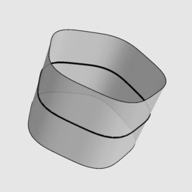
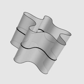
Figure 6. Two cylindrical membranes of the family with a five-fold symmetry corresponding to the values $\varrho=0.10300000000000001$ and $\varrho=0.6$ of the parameter $\varrho$.

Our result allow to deduce the existence of global solutions only when $\varrho\in[0,\varrho_{5})$ (i.e., if the directrix is strictly convex). Figure 6 reproduces the cylindrical membranes of the family with a five-fold symmetry corresponding to the values $\varrho=0.10300000000000001\in[0,\varrho_{5})$ and $\varrho=0.6\in(\varrho_{5},\varrho_{1,5})$. The global existence of the cylinder on the left can be inferred from Theorem 1. When the directrix has inflection points, then using Theorem 1, we can only foresee the vertical strips of the cylinder between the generating lines passing through two consecutive inflection points of the directrix curve (see Figure 7).

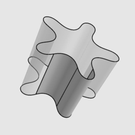
Figure 7. Two strips of the cylinder with $\upsilon=5$ and $\varrho=0.6$ which can be deduced from Theorem 1.

References

• [1] L. J. Alías, R. M. B. Chaves, and P. Mira, Björling problem for maximal surfaces in Lorentz-Minkowski space, Math. Proc. Cambridge Philos. Soc. 134 (2003), no. 2, 289–316.
• [2] J. A. Aledo, R. M. B. Chaves, and J. A. Gálvez, The Cauchy problem for improper affine spheres and the Hessian one equation, Trans. Amer. Math. Soc. 359 (2007), no. 9, 4183–4208.
• [3] R. L. Bishop, There is more than one way to frame a curve, Amer. Math. Monthly 82 (1975), 246–251.
• [4] W. Blaschke, Vorlesungen über Differentialgeometrie und geometrische Grundlagen von Einsteins Relativitätstheorie, B. 3, bearbeitet von G. Thomsen, J. Springer, Berlin, 1929.
• [5] D. Brander and J. F. Dorfmeister, The Björling problem for non-minimal constant mean curvature surfaces, Comm. Anal. Geom. 18 (2010), no. 1, 171–194.
• [6] D. Brander and M. Svensson, The geometric Cauchy problem for surfaces with Lorentzian harmonic Gauss maps, J. Differential Geom. 93 (2013), no. 1, 37–66.
• [7] R. L. Bryant, A duality theorem for Willmore surfaces, J. Differential Geom. 20 (1984), 23–53.
• [8] R. L. Bryant, S.-S. Chern, R. B. Gardner, H. L. Goldschmidt, and P. A. Griffiths, Exterior differential systems, MSRI Publications, 18, Springer-Verlag, New York, 1991.
• [9] R. L. Bryant and P. A. Griffiths, Reduction for constrained variational problems and $\int{\frac{1}{2}k^{2}ds}$, Amer. J. Math. 108 (1986), 525–570.
• [10] P. B. Canham, The minimum energy of bending as a possible explanation of the biconcave shape of the human red blood cell, J. Theor. Biol. 26 (1970), 61–81.
• [11] R. Capovilla, J. Guven, and E. Rojas, Hamilton’s equations for a fluid membrane: axial symmetry, J. Phys. A 38 (2005), 8201–8210.
• [12] E. Cartan, Les systèmes différentiels extérieurs et leurs applications géométriques, Hermann, Paris, 1945.
• [13] H. J. Deuling and W. Helfrich, The curvature elasticity of fluid membranes: A catalogue of vesicle shapes, J. Phys. (Paris) 37 (1976), 1335–1345.
• [14] E. Evans, Bending resistance and chemically induced moments in membrane bilayers, Biophys. J. 14 (1974), 923–931.
• [15] J. A. Gálvez and P. Mira, The Cauchy problem for the Liouville equation and Bryant surfaces, Adv. Math. 195 (2005), no. 2, 456–490.
• [16] R. E. Goldstein and D. M. Pertich, The Korteweg-de Vries hierarchy as dynamics of closed curves in the plane, Phys. Rev. Lett. 67 (1991), no. 23, 3203–3206.
• [17] P. A. Griffiths, Exterior differential systems and the calculus of variations, Progress in Mathematics, 25, Birkhäuser, Boston, 1982.
• [18] P. A. Griffiths and G. R. Jensen, Differential systems and isometric embeddings, Annals of Mathematics Studies, 114, Princeton University Press, Princeton, NJ, 1987.
• [19] W. Helfrich, Elastic properties of lipid bilayers: Theory and possible experiments, Z. Naturforsch. C 28 (1973), 693–703.
• [20] L. Hsu, R. Kusner, and J. Sullivan, Minimizing the squared mean curvature integral for surfaces in space forms, Experiment. Math. 1 (1992), no. 3, 191–207.
• [21] T. A. Ivey and J. M. Landsberg, Cartan for beginners: differential geometry via moving frames and exterior differential systems, Graduate Studies in Mathematics, 61, American Mathematical Society, Providence, RI, 2003.
• [22] R. Lipowsky, The conformation of membranes, Nature 349 (1991), 475–482.
• [23] F. C. Marques and A. Neves, Min-Max theory and the Willmore conjecture, Ann. of Math. (2) 179 (2014), no. 2, 683–782. See also arxiv.org/abs/1202.6036, 2012.
• [24] E. Musso, Congruence curves of the Goldstein-Petrich flows. Harmonic maps and differential geometry, 99–113, Contemp. Math., 542, Amer. Math. Soc., Providence, RI, 2011.
• [25] E. Musso and L. Nicolodi, On the Cauchy problem for the integrable system of Lie minimal surfaces, J. Math. Phys. 46 (2005), no. 11, 3509–3523.
• [26] E. Musso and L. Nicolodi, Tableaux over Lie algebras, integrable systems, and classical surface theory, Comm. Anal. Geom. 14 (2006), no. 3, 475–496.
• [27] E. Musso and L. Nicolodi, A class of overdetermined systems defined by tableaux: involutiveness and the Cauchy problem, Phys. D 229 (2007), no. 1, 35–42.
• [28] E. Musso and L. Nicolodi, Differential systems associated with tableaux over Lie algebras. In Symmetries and overdetermined systems of partial differential equations, 497–513, IMA Vol. Math. Appl., 144, Springer, New York, 2008.
• [29] K. Nakayama, H. Segur, M. Wadati, Integrability and the motion of curves, Phys. Rev. Lett. 69 (1992), no. 18, 2603–2606.
• [30] J. C. C. Nitsche, Lecture on Minimal Surface, Vol. 1, Cambridge University Press, Cambridge, 1989.
• [31] J. C. C. Nitsche, Boundary value problems for variational integrals involving surface curvatures, Quart. Appl. Math. 51 (1993), 363–387.
• [32] Z. C. Ou-Yang and W. Helfrich, Instability and deformation of a spherical vesicle by pressure, Phys. Rev. Lett. 59 (1987), 2486–2488.
• [33] Z. C. Ou-Yang and W. Helfrich, Bending energy of vesicle membranes: General expressions for the first, second, and third variation of the shape energy and applications to spheres and cylinders. Phys. Rev. A. 39 (1989), 5280–5288.
• [34] Z. C. Ou-Yang, J. X. Liu, and Y. Z. Xie, Geometric Methods in the Elastic Theory of Membranes in Liquid Crystal Phases, World Scientific, Singapore, 1999.
• [35] M. A. Peterson, Geometrical methods for the elasticity theory of membranes, J. Math. Phys. 26 (1985), no. 4, 711–717.
• [36] U. Seifert, Configurations of fluid membranes and vesicles, Adv. Phys. 46 (1997), 1–137.
• [37] D. J. Steigmann, Fluid films with curvature elasticity, Arch. Rational Mech. Anal. 150 (1999), 127–152.
• [38] D. J. Steigmann, E. Baesu, R. E. Rudd, J. Belak, and M. McElfresh, On the variational theory of cell-membrane equilibria, Interfaces Free Bound. 5 (2003), 357–366.
• [39] G. Thomsen, Über konforme Geometrie I: Grundlagen der konformen Flächentheorie, Hamb. Math. Abh. 3 (1923), 31–56.
• [40] S. Tek, Modified Korteweg-de Vries surfaces, J. Math. Phys. 48 (2007), no. 1, 13505–13521.
• [41] Z. C. Tu and Z. C. Ou-Yang, A geometric theory on the elasticity of bio-membranes, J. Phys. A 37 (2004), 11407–11429.
• [42] J. L. van Hemmen and C. Leibold, Elementary excitations of biomembranes: Differential geometry of undulations in elastic surfaces, Phys. Rep. 444 (2007), no. 2, 51–99.
• [43] V. M. Vassilev, P. A. Djondjorov, and I. M. Mladenov, Cylindrical equilibrium shapes of fluid membranes, J. Phys. A 41 (2008), no. 43, 435201–435216.
• [44] T. J. Willmore, Riemannian geometry, Clarendon Press, Oxford, 1993.
• [45] S.-G. Zhang and Z. C. Ou-Yang, Periodic cylindrical surface solution for fluid bilayer membranes, Phys. Rev. E 55 (1996), no. 4, 4206–4208.