The Lagrangian Cubic Equation

Abstract.

Let $M$ be a closed symplectic manifold and $L\subset M$ a Lagrangian submanifold. Denote by $[L]$ the homology class induced by $L$ viewed as a class in the quantum homology of $M$. The present paper is concerned with properties and identities involving the class $[L]$ in the quantum homology ring. We also study the relations between these identities and invariants of $L$ coming from Lagrangian Floer theory. We pay special attention to the case when $L$ is a Lagrangian sphere.

1. Introduction and main results

Let $M^{2n}$ be a closed symplectic $2n$-dimensional manifold. Assume further that $M$ is monotone with minimal Chern number $C_{M}$ (see §2.1 below for the definitions). Denote by $QH(M)$ the quantum homology of $M$ with coefficients in the ring $\mathbb{\mathbb{Z}}[q]$, where the degree of the variable $q$ is $|q|=-2$. Denote by $*$ the quantum product on $QH(M)$ and for a class $a\in QH(M)$, $k\in\mathbb{N}$, we write $a^{*k}$ for the $k$’th power of $a$ with respect to this product.

Let $S\subset M$ be an oriented Lagrangian $n$-sphere. Denote by $[S]\in QH_{n}(M)$ the homology class represented by $S$ in the quantum homology of $M$. Our first result shows that $[S]$ always satisfies a cubic or quadratic equation of a very specific type:

Theorem A.

1. If $n=$ odd then $[S]*[S]=0$.

2. Assume $n=$ even. Then:

   1. If $C_{M}|n$ then there exists a unique $\gamma_{S}\in\mathbb{Z}$ such that $[S]^{*3}=\gamma_{S}[S]q^{n}$. If we assume in addition that $2C_{M}\centernot|n$, then $\gamma_{S}$ is divisible by $4$, while if $2C_{M}|n$ then $\gamma_{S}$ is either $0(\bmod\,4)$ or $1(\bmod\,4)$.

   2. If $C_{M}\centernot|n$ then $[S]^{*3}=0$.

The proof of Theorem A, given in §3.2, follows from a simple argument involving Lagrangian Floer homology. The cases (1), (2ii) are particularly simple, whereas case (2i) splits into two sub-cases:

1. $2C_{M}|n$.

2. $C_{M}|n$, but $2C_{M}\centernot|n$.

We will see below that out of these two sub-cases the most interesting is (2i-a). In that case the constant $\gamma_{S}$ has other interpretations coming from Floer theory and enumerative geometry of holomorphic disks. These will be explained in detail in the sequel.

Remark 1.A.

1. When $n$ is even it is easy to see that $[S]\in H_{n}(M)$ is neither $0$ nor a torsion class. Therefore in that case $\gamma_{S}$ is uniquely determined.

2. Points (1) and (2ii) of the theorem cover the symplectically aspherical case (i.e. $[\omega]|_{\pi_{2}(M)}=0$) if we set $C_{M}=\infty$. Of course, the statement in that case is completely obvious.

3. A version of Theorem A also holds in the non-monotone case for Lagrangian 2-spheres, the precise statement can be found in §8.

4. Theorem A continues to hold also when $S$ is a $\mathbb{Z}$-homology sphere, except possibly when $2C_{M}|n$. The difference between the case $2C_{M}|n$ and the others is that in that case $[S]$ a priori satisfies only the cubic equation (1) from Theorem B below. For the vanishing of the coefficient of $[S]^{*2}$ we will use the Dehn twist along $S$ (see Corollary C and the short discussion after it), hence we need to assume that $S$ is diffeomorphic to a sphere. At the same time we are not aware of interesting computable examples where $S$ is a $\mathbb{Z}$-homology sphere yet not a genuine sphere.

For the rest of the introduction we concentrate on case (2i-a) and its possible generalizations. Assume from now on that $L\subset M$ is a Lagrangian submanifold (not necessarily a sphere). Denote by $HF_{*}(L,L)$ the self Floer homology of $L$ with coefficients in $\mathbb{Z}$. See §2 for the Floer theoretical setting. In what follows we will recurringly appeal to the following set of assumptions or to a subset of it:

Assumption $\mathscr{L}$.

1. $L$ is closed (i.e. compact without boundary). Furthermore $L$ is monotone with minimal Maslov number $N_{L}$ that satisfies $N_{L}\mid n$ (see §2.1 for the definitions). Set $\nu=n/N_{L}$.

2. $L$ is oriented. Moreover we assume that $L$ is spinable (i.e. can be endowed with a spin structure).

3. $HF_{n}(L,L)$ has rank $2$.

4. Write $\chi=\chi(L)$ for Euler-characteristic of $L$. We assume that $\chi\neq 0$.

Note that conditions $(1)$ and $(2)$ together imply that $n=$ even, since orientable Lagrangians have $N_{L}=$ even. Independently, conditions $(2)$ and $(4)$ also imply that $n=$even. As we will see later there are many Lagrangian submanifolds that satisfy Assumption $\mathscr{L}$ – for example, even dimensional Lagrangian spheres in monotone symplectic manifolds $M$ with $2C_{M}|n$. See §1.3 and §5 for more examples.

Unless otherwise stated, from now on we implicitly assume all Lagrangian submanifolds to be connected.

1.1. The Lagrangian cubic equation

Here we need to work with $\mathbb{Q}$ as the base ring. Denote by $QH(M;\mathbb{Q}[q])$ the quantum homology of $M$ with coefficients in the ring $\mathbb{Q}[q]$. Given an oriented Lagrangian submanifold $L\subset M$ denote by $[L]\in QH_{n}(M;\mathbb{Q}[q])$ its homology class in the quantum homology of the ambient manifold $M$. We will also make use of the following notation $\varepsilon=(-1)^{n(n-1)/2}$.

Our first result is the following.

Theorem B (The Lagrangian cubic equation).

Let $L\subset M$ be a Lagrangian submanifold satisfying assumption $\mathscr{L}$. Then there exist unique constants $\sigma_{L}\in\tfrac{1}{\chi^{2}}\mathbb{\mathbb{Z}}$, $\tau_{L}\in\tfrac{1}{\chi^{3}}\mathbb{Z}$ such that the following equation holds in $QH(M;\mathbb{Q}[q])$:

(1) $$[L]^{*3}-\varepsilon\chi\sigma_{L}[L]^{*2}q^{n/2}-\chi^{2}\tau_{L}[L]q^{n}=0.$$

If $\chi$ is square-free then $\sigma_{L}\in\tfrac{1}{\chi}\mathbb{Z}$ and $\tau_{L}\in\tfrac{1}{\chi^{2}}\mathbb{Z}$. Moreover, the constant $\sigma_{L}$ can be expressed in terms of genus $0$ Gromov-Witten invariants as follows:

(2) $$\sigma_{L}=\frac{1}{\chi^{2}}\sum_{A}GW^{M}_{A,3}([L],[L],[L]),$$

where the sum is taken over all classes $A\in H_{2}(M)$ with $\langle c_{1},A\rangle=n/2$.

In §3 we will prove a more general result concerning a Lagrangian submanifold $L$ and an arbitrary class $c\in H_{n}(M)$ which satisfies $c\cdot[L]\neq 0$. We will prove that they satisfy a mixed equation of degree three involving $[L]$ and $c$. Equation (1) is the special case $c=[L]$.

Here is an immediate corollary of Theorem B:

Corollary C.

Let $L\subset M$ be a Lagrangian submanifold satisfying Assumption $\mathscr{L}$. Assume in addition that there exists a symplectic diffeomorphism $\varphi:M\longrightarrow M$ such that $\varphi_{*}([L])=-[L]$. Then $\sigma_{L}=0$, hence equation (1) reads in this case:

$$[L]^{*3}-\chi^{2}\tau_{L}[L]q^{n}=0.$$

When $L$ is a Lagrangian sphere in a symplectic manifold $M$ with $2C_{M}|n$ then point (2i) of Theorem A follows from Corollary C. Indeed, we can take $\varphi$ to be the Dehn twist along $L$. The Picard-Lefschetz formula (see e.g. [Dim, AGLV]) gives $\varphi_{*}([L])=-[L]$ since $n=\dim L$ is even and $\chi=2$. Corollary C then implies that $\sigma_{L}=0$ (and we have $\gamma_{L}=4\tau_{L}$). Note that in this case we have $\tau_{L}\in\tfrac{1}{4}\mathbb{Z}$.

Proof of Corollary C.

Applying $\varphi_{*}$ to the equation (1) and comparing the result to (1) yields $\varepsilon\chi\sigma_{L}[L]^{*2}=0$. Since $\chi\neq 0$ it follows that $\sigma_{L}[L]^{*2}=0$. But $[L]\cdot[L]=\varepsilon\chi\neq 0$, hence $[L]^{*2}\neq 0$. This implies that $\sigma_{L}=0$. ∎

1.2. The discriminant

Let $A$ be a quadratic algebra over $\mathbb{Z}$. By this we mean that $A$ is a commutative unital ring such that $\mathbb{Z}$ embeds as a subring of $A$, $\mathbb{Z}\to A$, and furthermore that $A/\mathbb{Z}\cong\mathbb{Z}$. Thus the underlying additive abelian group of $A$ is a free abelian group of rank $2$. Pick a generator $p\in A/\mathbb{Z}$ so that $A/\mathbb{Z}=\mathbb{Z}p$. We have the following exact sequence:

(3) $$0\longrightarrow\mathbb{Z}\longrightarrow A\xrightarrow{\;\;\epsilon\;\;}\mathbb{Z}p\longrightarrow 0,$$

where the first map is the ring embedding and $\epsilon$ is the obvious projection. Choose a lift $x\in A$ of $p$, i.e. $\epsilon(x)=p$. Then additively we have $A\cong\mathbb{Z}x\oplus\mathbb{Z}$. With these choices there exist $\sigma(p,x),\tau(p,x)\in\mathbb{Z}$ such that

$$x^{2}=\sigma(p,x)x+\tau(p,x).$$

The integers $\sigma(p,x),\tau(p,x)$ depend on the choices of $p$ and of $x$. However, a simple calculation (see §2.5.1) shows that the following expression

(4) $$\Delta_{A}:=\sigma(p,x)^{2}+4\tau(p,x)\in\mathbb{Z}$$

is independent of $p$ and $x$, hence is an invariant of the isomorphism type of $A$. In fact in §2.5.2 we show that $\Delta_{A}$ determines the isomorphism type of $A$. We call $\Delta_{A}$ the discriminant of $A$.

Remarks.

1. Another description of $\Delta_{A}$ is the following. Write $A$ as $A\cong\mathbb{Z}[T]/(f(T))$, where $f(T)\in\mathbb{Z}[T]$ is a monic quadratic polynomial. Then $\Delta_{A}$ is the discriminant of $f(T)$ (and is independent of the choice of $f(T)$). In particular $A_{\mathbb{C}}:=A\otimes\mathbb{C}$ is semi-simple iff $\Delta_{A}\neq 0$.

2. When $\Delta_{A}$ is not a square $A_{\mathbb{Q}}:=A\otimes\mathbb{Q}$ is a quadratic number field. The discriminant $\Delta_{A}$ is related to the discriminant of $A_{\mathbb{Q}}$ as defined in number theory.

3. It is easy to see from (4) that the only values $\Delta_{A}(\bmod\,4)$ can assume are $0$ and $1$.

Let $L$ be a Lagrangian submanifold satisfying conditions $(1)-(3)$ of Assumption $\mathscr{L}$ and choose a spin structure on $L$ compatible with its orientation. Consider $A=HF_{n}(L,L)$ endowed with the Donaldson product

$$*:HF_{n}(L,L)\otimes HF_{n}(L,L)\longrightarrow HF_{n}(L,L),\quad a\otimes b\longmapsto a*b.$$

Recall that $A$ is a unital ring with a unit which we denote by $e_{L}\in HF_{n}(L,L)$. The conditions $(1)-(3)$ of Assumption $\mathscr{L}$ ensure that $A$ is a quadratic algebra over $\mathbb{Z}$. (In case $A$ has torsion we just replace it by $A/T$, where $T$ is its torsion ideal.) Denote by $\Delta_{L}$ the discriminant of $A$, $\Delta_{L}:=\Delta_{A}$ as defined in (4). (We suppress here the dependence on the spin structure, as we will soon see that in our case $\Delta_{L}$ does not depend on it.)

The following theorem shows that the discriminant $\Delta_{L}$ depends only on the class $[L]\in QH_{n}(M)$ and can be computed by means of the ambient quantum homology of $M$.

Theorem D.

Let $L\subset M$ be a Lagrangian submanifold satisfying Assumption $\mathscr{L}$. Let $\sigma_{L},\tau_{L}\in\mathbb{Q}$ be the constants from the cubic equation (1) in Theorem B. Then

$$\Delta_{L}=\sigma_{L}^{2}+4\tau_{L}.$$

The proof appears in §3.

Remarks.

1. Warning: The pair of coefficients $\sigma_{L},\tau_{L}$ and $\sigma(p,x),\tau(p,x)$ should not be confused. The first pair is always uniquely determined by $[L]$ and can be read off the ambient quantum homology of $M$ via the cubic equation (1). In contrast, the second pair $\sigma(p,x),\tau(p,x)$ are defined via Lagrangian Floer homology and strongly depend on the choice of the lift $x$ of $p$. For example, we have seen that if $L$ is a sphere then $\sigma_{L}=0$, but as we will see later (e.g. in §4) for some (useful) choices of $x$ we have $\sigma(p,x)\neq 0$. Additionally, $\sigma(p,x),\tau(p,x)\in\mathbb{Z}$ while $\sigma_{L},\tau_{L}\in\mathbb{Q}$. Still, the two pairs of coefficients are related in that $\sigma(p,x)^{2}+4\tau(p,x)=\sigma_{L}^{2}+4\tau_{L}=\Delta_{L}$.

   As we will see in the proof of Theorem D, the coefficients $\sigma_{L},\tau_{L}$ do occur as $\sigma(p,x_{0}),\tau(p,x_{0})$ but for a special choice of $x_{0}$, which however requires working over $\mathbb{Q}$.

2. A different version of the discriminant $\Delta_{L}$ was previously defined and studied by Biran-Cornea in [BC5]. In that paper the discriminant occurs as an invariant of a quadratic form defined on $H_{n-1}(L)$ via Floer theory. In the case $L$ is a $2$-dimensional Lagrangian torus the discriminant from [BC5] and $\Delta_{L}$, as defined above, happen to coincide due to the associativity of the product of $HF_{n}(L,L)$. Moreover, in dimension $2$, $\Delta_{L}$ has an enumerative description in terms of counting holomorphic disks with boundary on $L$ which satisfy certain incidence conditions. This description continues to hold also for $2$-dimensional Lagrangian spheres with $N_{L}=2$ (or more generally for all $2$-dimensional Lagrangian submanifolds satisfying Assumption $\mathscr{L}$) and the proof is the same as in [BC5].

3. Since $\sigma_{L},\tau_{L}$ do not depend on the spin structure chosen for $L$ (although $\sigma(p,x)$ and $\tau(p,x)$ do) it follows from Theorem D that $\Delta_{L}$ does not depend on that choice either. As for the orientation on $L$, if we denote $\bar{L}$ the Lagrangian $L$ with the opposite orientation then it follows from Theorem B that $\sigma_{\bar{L}}=-\sigma_{L}$ and $\tau_{\bar{L}}=\tau_{L}$. In particular $\Delta_{\bar{L}}=\Delta_{L}$.

The next theorem is concerned with the behavior of the discriminant under Lagrangian cobordism. We refer the reader to [BC6] for the definitions.

Theorem E.

Let $L_{1},\ldots,L_{r}\subset M$ be monotone Lagrangian submanifolds, each satisfying conditions $(1)$ – $(3)$ of Assumption $\mathscr{L}$. Let $V^{n+1}\subset\mathbb{R}^{2}\times M$ be a connected monotone Lagrangian cobordism whose ends correspond to $L_{1},\ldots,L_{r}$ and assume that $V$ admits a spin structure. Denote by $N_{V}$ the minimal Maslov number of $V$ and assume that:

1. $H_{jN_{V}}(V,\partial V)=0$ for every $j$.

2. $H_{1+jN_{V}}(V)=0$ for every $j$.

Then $\Delta_{L_{1}}=\cdots=\Delta_{L_{r}}$. Moreover if $r\geq 3$ then $\Delta_{L_{i}}$ is a perfect square for every $i$.

The proof is given in §4. As a corollary we obtain:

Corollary F.

Let $(M,\omega)$ be a monotone symplectic manifold with $2C_{M}\mid n$, where $C_{M}$ is the minimal Chern number of $M$. Let $L_{1},L_{2}\subset M$ be two Lagrangian spheres that intersect transversely at exactly one point. Then $\Delta_{L_{1}}=\Delta_{L_{2}}$ and moreover this number is a perfect square.

We will in fact prove a stronger result in §4.1 (see Corollary 4.1.A).

1.3. Examples

We begin with a topological criterion that assures that condition (3) in Assumption $\mathscr{L}$ is satisfied. This provides us with examples of Lagrangian submanifolds to which the theory applies.

Proposition G.

Let $L\subset M$ be an oriented Lagrangian submanifold satisfying condition $(1)$ of Assumption $\mathscr{L}$. Assume in addition that:

1. $[L]\neq 0\in H_{n}(M;\mathbb{Q})$ (this is satisfied e.g. when $\chi(L)\neq 0$).

2. $H_{jN_{L}}(L)=0$ for every $0<j<\nu$.

Then condition $(3)$ in Assumption $\mathscr{L}$ is satisfied too. In particular Lagrangian spheres $L$ that satisfy condition $(1)$ of Assumption $\mathscr{L}$ satisfy the other three conditions in Assumption $\mathscr{L}$.

The proof appears in §2.3.

We now provide a sample of examples. More details will be given in §5

1.3.1. Lagrangian spheres in blow-ups of $\mathbb{C}P^{2}$

Let $(M_{k},\omega_{k})$ be the monotone symplectic blow-up of ${\mathbb{C}}P^{2}$ at $2\leq k\leq 6$ points. We normalize $\omega_{k}$ so that it is cohomologous to $c_{1}$. Denote by $H\in H_{2}(M_{k})$ the homology class of a line not passing through the blown up points and by $E_{1},\ldots,E_{k}\in H_{2}(M_{k})$ the homology classes of the exceptional divisors over the blown up points. With this notation the Poincaré dual of the cohomology class of the symplectic form $[\omega_{k}]\in H^{2}(M_{k})$ satisfies

$$PD[\omega_{k}]=PD(c_{1})=3H-E_{1}-\cdots-E_{k}.$$

The Lagrangian spheres $L\subset M_{k}$ lie in the following homology classes (see §5.1 for more details):

1. For $k=2$: $\pm(E_{1}-E_{2})$.

2. For $2\leq k\leq 5$: $\pm(E_{i}-E_{j})$, $i<j$, and $\pm(H-E_{i}-E_{j}-E_{l})$ with $i<j<l$.

3. For $k=6$ we have the same homology classes as in $(2)$ and in addition the class $\pm(2H-E_{1}-\cdots-E_{6})$.

Note that all these Lagrangian spheres satisfy Assumption $\mathscr{L}$ since $N_{L}=2$.

The discriminants of these Lagrangian spheres are gathered in Table 1, the detailed computations being postponed to §5. The column under $\lambda_{L}$ will be explained in §2.4.

	$[L]$	$\Delta_{L}$	$\lambda_{L}$
$M_{2}$	$\pm(E_{1}-E_{2})$	5	-1
$M_{3}$	$\pm(E_{i}-E_{j})$	4	-2
	$\pm(H-E_{1}-E_{2}-E_{3})$	-3	-3
$M_{4}$	$\pm(E_{i}-E_{j})$	1	-3
	$\pm(H-E_{i}-E_{j}-E_{l})$	1	-3
$M_{5}$	$\pm(E_{i}-E_{j})$	0	-4
	$\pm(H-E_{i}-E_{j}-E_{l})$	0	-4
$M_{6}$	$\pm(E_{i}-E_{j})$	0	-6
	$\pm(H-E_{i}-E_{j}-E_{l})$	0	-6
	$\pm(2H-E_{1}-\ldots-E_{6})$	0	-6

Table 1. Classes representing Lagrangian spheres and their discriminants.

The Lagrangian spheres in the three homology classes $E_{i}-E_{j}$, $i<j$, of $M_{3}$ all have the same discriminant. This can also be seen by noting that one can choose three Lagrangian spheres $L_{1},L_{2},L_{3}$, one in each of these homology classes so that every pair of them intersects transversely at exactly one point. The equality of their discriminants as well (as the fact that they are perfect squares) follows then by Corollary F. We elaborate more on these examples in §5.

1.3.2. Lagrangian spheres in hypersurfaces of ${\mathbb{C}}P^{n+1}$

Let $M^{2n}\subset\mathbb{C}P^{n+1}$ be a hypersurface of degree $d\leq n+1$ endowed with the induced symplectic form. By the assumption on $d$, $M$ is monotone (in fact Fano) and the minimal Chern number is $C_{M}=n+2-d$. Note that when $d\geq 2$, $M$ contains Lagrangian spheres. Assume further that $n\geq 3$, and $d\geq 3$. Let $L\subset M$ be a Lagrangian sphere, hence $[L]$ belongs to the primitive homology of $M$ (see [GH, Voi]). Using the description of the quantum homology of $M$ from [CJ, Giv] we obtain $[L]^{*3}=0$.

Whenever $n$ is a multiple of $2C_{M}=2(n+2-d)$ the Lagrangian spheres $L\subset M$ satisfy Assumption $\mathscr{L}$, hence the discriminant is defined and we obtain $\Delta_{L}=0$.

Consider now the case $d=2$, i.e. $M$ is the quadric of complex dimension $n$, and let $S\subset M$ be a Lagrangian sphere. We have $C_{M}=n$, so case (2i) of Theorem A applies. If $n=$ odd, then $H_{n}(M)=0$, hence $[S]=0$. If $n=$ even, then from the quantum product in the quadric we obtain:

$$[S]^{*3}=(-1)^{\frac{n(n-1)}{2}+1}4[S]q^{n}.$$

More details on all the above calculations are given in §5.

Acknowledgments

We would like to thank Jean-Yves Welschinger for a discussion convincing us that all Lagrangian tori in symplectic $4$-manifolds with $b_{2}^{+}=1$ are null-homologous.

Organization of the paper

The rest of the paper is organized as follows. In §2 we briefly recall the necessary ingredients from Lagrangian Floer and quantum homologies used in the sequel. In §2.5 we also give more details on the discriminant. §3 is devoted to the Lagrangian cubic equation. We prove in that section more general versions of Theorems B and D. Then in §3.2 we prove Theorem A. We also prove in §3.3 additional corollaries derived from these theorems. In §4 we study the discriminant in the realm of Lagrangian cobordism and prove Theorem E and Corollary F. §5 is dedicated to examples. We briefly explain how to construct Lagrangian spheres in various homology classes on symplectic Del Pezzo surfaces and carry out the calculation of the discriminants of those Lagrangians. We discuss some higher dimensional examples too. In §6 we explain an extension of the discriminant and the Lagrangian cubic equation over a more general ring of coefficients that takes into account the different homology classes of the holomorphic curves that contribute to our invariants. In §6.2 we recalculate some of the examples from §5 over this ring. In §7 we discuss the relation of the discriminant to the enumerative geometry of holomorphic disks. Finally, in §8 we consider the non-monotone case and state a version of Theorem A for not necessarily monotone Lagrangian 2-spheres.

2. Lagrangian Floer theory

Here we briefly recall some ingredients from Floer theory that are relevant for this paper. These include Lagrangian Floer homology and especially its realization as Lagrangian quantum homology (a.k.a pearl homology). The reader is referred to [Oh1, Oh2, FOOO1, FOOO2, BC4, BC5] for more details.

2.1. Monotone symplectic manifolds and Lagrangians

Let $(M,\omega)$ be a symplectic manifold. Denote by $c_{1}\in H^{2}(M)$ the first Chern class of the tangent bundle $T(M)$ of $M$. Denote by $H_{2}^{S}(M)$ the image of the Hurewicz homomorphism $\pi_{2}(M)\longrightarrow H_{2}(M)$. We call $(M,\omega)$ monotone if there exists a constant $\vartheta>0$ such that

$$A_{\omega}=\vartheta I_{c_{1}},$$

where $A_{\omega}:H_{2}^{S}(M)\longrightarrow\mathbb{R}$ is the homomorphism defined by integrating $\omega$ over spherical classes and $I_{c_{1}}$ is viewed as a homomorphism $H_{2}^{S}(M)\longrightarrow\mathbb{Z}$. We denote by $C_{M}$ the positive generator of the subgroup $\textnormal{image\,}I_{c_{1}}\subset\mathbb{Z}$ so that $\textnormal{image\,}I_{c_{1}}=C_{M}\mathbb{Z}$. If $\textnormal{image\,}I_{c_{1}}=0$ we set $C_{M}=\infty$.

$L\subset M$ a Lagrangian submanifold. Denote by $H_{2}^{D}(M,L)$ the image of the Hurewicz homomorphism $\pi_{2}(M,L)\longrightarrow H_{2}(M,L)$. We say that $L$ is monotone if there exists a constant $\rho>0$ such that

$$A_{\omega}=\rho\mu,$$

where $A_{\omega}:H_{2}^{D}(M,L)\longrightarrow\mathbb{R}$ is the homomorphism defined by integrating $\omega$ over homology classes and $\mu:H_{2}^{D}(M,L)\longrightarrow\mathbb{Z}$ is the Maslov index homomorphism. We denote by $N_{L}$ the positive generator of the subgroup $\textnormal{image\,}\mu\subset\mathbb{Z}$ so that $\textnormal{image\,}\mu=N_{L}\mathbb{Z}$.

Finally, denote by $j:H_{2}^{S}(M)\longrightarrow H_{2}^{D}(M,L)$ the obvious homomorphism. Then we have $\mu(j(A))=2I_{c_{1}}(A)$ for every $A\in H_{2}^{S}(M)$. Therefore, if $L$ is a monotone Lagrangian and $I_{c_{1}}\neq 0$ then $(M,\omega)$ is also monotone and we have $N_{L}\mid 2C_{M}$. When $\pi_{1}(L)=\{1\}$ we actually have $N_{L}=2C_{M}$.

2.2. Floer homology and Lagrangian quantum homology

Let $L\subset M$ be a closed monotone Lagrangian submanifold with $2\leq N_{L}\leq\infty$. Under the additional assumptions that $L$ is spin one can define the self Floer homology $HF(L,L)$ with coefficients in $\mathbb{Z}$. This group is cyclically graded, with grading in $\mathbb{Z}/N_{L}\mathbb{Z}$.

From the point of view of the present paper it is more natural to work with Lagrangian quantum homology $QH(L)$ rather than with the Floer homology $HF(L,L)$. This is justified by the fact that for an appropriate choice of coefficients we have an isomorphism of rings $QH(L)\cong HF(L,L)$. The advantage of $QH(L)$ in our context is that it bears a simple and explicit relation to the singular homology $H(L)$ of $L$. For example, under certain circumstances (relevant for our considerations) and with the right coefficient ring, $QH(L)$ can be viewed as a deformation of the singular homology ring $H(L)$ endowed with the intersection product.

We will now summarize the most basic properties of Lagrangian quantum homology. The reader is referred to [BC4, BC5] for the foundations of the theory.

Denote by $\Lambda=\mathbb{Z}[t^{-1},t]$ the ring of Laurent polynomials over $\mathbb{Z}$ graded so that the degree of $t$ is $|t|=-N_{L}$. We denote by $QH^{\#}(L)$ the Lagrangian quantum homology of $L$ with coefficients in $\mathbb{Z}$ and by $QH(L;\Lambda)$ the one with coefficients in $\Lambda$. Thus $QH^{\#}(L)$ is cyclically graded modulo $N_{L}$ and $QH(L;\Lambda)$ is $\mathbb{Z}$-graded and $N_{L}$-periodic, i.e. $QH_{i}(L;\Lambda)\cong QH_{i-N_{L}}(L;\Lambda)$, the isomorphism being given by multiplication by $t$. And we have $QH_{i}(L;\Lambda)\cong QH^{\#}_{i\pmod{N_{L}}}(L)$, hence the grading on $QH(L;\Lambda)$ is an unwrapping of the cyclic grading of $QH^{\#}(L)$. Sometimes, when the context is clear we will write $QH(L)$ for $QH(L;\Lambda)$.

The Lagrangian quantum homology has the following algebraic structures. There exists a quantum product

$$QH_{i}(L;\Lambda)\otimes QH_{j}(L;\Lambda)\longrightarrow QH_{i+j-n}(L;\Lambda),\quad\alpha\otimes\beta\longmapsto\alpha*\beta,$$

which turns $QH(L;\Lambda)$ into a unital associative ring with unity $e_{L}\in QH_{n}(L;\Lambda)$.

We now briefly recall relations between the Lagrangian and ambient quantum homologies. Denote by $R=\mathbb{Z}[q^{-1},q]$ the ring of Laurent polynomials in the variable $q$, whose degree we set to be $|q|=-2$. Denote by $QH(M;R)$ the quantum homology of $M$ with coefficients in $R$, endowed with the quantum product $*$. The Lagrangian quantum homology $QH(L;\Lambda)$ is a module over the subring $QH(M;\Lambda)\subset QH(M;R)$, where $\Lambda$ is embedded in $R$ by $t\mapsto q^{N_{L}/2}$. We denote this operation by

$$QH_{i}(M;\Lambda)\otimes QH_{j}(L;\Lambda)\longrightarrow QH_{i+j-2n}(L;\Lambda),\quad a\otimes\alpha\longmapsto a*\alpha.$$

The reason for using the same notation $*$ as for the quantum product on $L$ is that the module operation is compatible with the latter in the following sense:

(5) $$c*(\alpha*\beta)=(c*\alpha)*\beta=(-1)^{(2n-|c|)(n-|\alpha|)}\alpha*(c*\beta),$$

for every $c\in QH(M;\Lambda)$, $\alpha,\beta\in QH(L;\Lambda)$. Note that the sign conventions in (5) are compatible with the standard sign conventions for the intersection product in singular homology.

The proof of identity (5) has been carried out in [BC2, BC4] over $\mathbb{Z}_{2}$ (hence without taking signs into account), and the same proof carries over in a straightforward way over $\mathbb{Z}$ using [BC5]. Thus $QH(L;\Lambda)$ is an algebra (in the graded sense) over $QH(M;\Lambda)$.

There is also a quantum inclusion map

$$i_{L}:QH_{i}(L;\Lambda)\longrightarrow QH_{i}(M;\Lambda),$$

which is linear over the ring $QH(M;\Lambda)$, i.e. $i_{L}(c*\alpha)=c*i_{L}(\alpha)$ for every $c\in QH(M;\Lambda)$ and $\alpha\in QH(L;\Lambda)$. An important property of $i_{L}$ is that $i_{L}(e_{L})=[L]$, see [BC5].

Next there is an augmentation morphism

$$\epsilon_{L}:QH(L;\Lambda)\longrightarrow\Lambda,$$

which is induced from a chain level extension of the classical augmentation. The augmentation satisfies the following identity, see [BC4]:

(6) $$\langle PD(h),i_{L}(\alpha)\rangle=\epsilon_{L}(h*\alpha),\quad\forall h\in H_{*}(M),\;\alpha\in QH(L;\Lambda),$$

where $PD$ stands for Poincaré duality and $\langle\cdot,\cdot\rangle$ denotes the Kronecker pairing extended over $\Lambda$ in an obvious way. Sometimes it will be more convenient to view the augmentation as a map

$$\widetilde{\epsilon}_{L}:QH(L;\Lambda)\longrightarrow H_{0}(L;\Lambda)=\Lambda[\textnormal{point}].$$

This augmentations $\epsilon_{L}$ and $\widetilde{\epsilon}_{L}$ descend also to $QH^{\#}(L)$ and by slight abuse of notation we denote them the same:

$$\epsilon_{L}:QH^{\#}(L)\longrightarrow\mathbb{Z},\quad\widetilde{\epsilon}_{L}:QH^{\#}(L)\longrightarrow H_{0}(L).$$

As mentioned earlier we will not really use Floer homology in this paper, but Lagrangian quantum homology instead. The justification for replacing $HF(L,L)$ by $QH^{\#}(L)$ is due to the PSS isomorphism

$$PSS:HF_{*}(L,L)\longrightarrow QH^{\#}_{*}(L).$$

This is a ring isomorphism which intertwines the Donaldson product and the quantum product on $QH^{\#}(L)$. A version of $PSS$ works with coefficients in $\Lambda$ too. For more details on the PSS isomorphism see [Alb, BC1, CL, BC4]. See also [HL, HLL] for the extension to $\mathbb{Z}$-coefficients.

Finally, we remark that everything mentioned above in this section continues to hold (with obvious modifications) also with other choices of base rings, replacing $\mathbb{Z}$ by $\mathbb{Q}$ or $\mathbb{C}$. For $K=\mathbb{Q}$ or $\mathbb{C}$ we write $\Lambda_{K}=K[t^{-1},t]$, $R_{K}=K[q^{-1},q]$ for the associated rings of Laurent polynomials and by $HF(L,L;\Lambda_{K})$, $QH(L;\Lambda_{K})$ and $QH(M;R_{K})$ the corresponding homologies. Sometimes it will be useful to drop the Laurent polynomial rings $\Lambda_{K}$ and $R_{K}$ and simply work with $HF(L,L;K)$, $QH(L;K)$ and $QH(M;K)$. Another variation that will be used in the sequel is to replace $\Lambda_{K}$ and $R_{K}$ by polynomial rings (rather than Laurent polynomials), i.e. work with coefficients in $\Lambda^{+}_{K}=K[t]$ and $R^{+}_{K}=K[q]$. See [BC4, BC3, BC5] for a detailed account on this choice of coefficients. When the base ring $K$ is obvious we will abbreviate $Q^{+}H(L):=QH(L;\Lambda^{+}_{K})$ and similarly for $Q^{+}H(M)$. (There has been only one exception to this notation. In the introduction §1 we denoted by $QH(M)$ the quantum homology $QH(M;R^{+})$ in order to facilitate the notation, but henceforth we will stick to the notation we have just described.) The homologies of the type $Q^{+}H$ will be called positive quantum homologies. Again, everything described above continues to work for the positive versions of quantum homologies with one important exception: the PSS isomorphism does not hold over $\Lambda^{+}_{K}$ (at least not for a straightforward version of Floer homology).

2.3. Proof of Proposition G

The proof appeals to a spectral sequence for calculating Lagrangian quantum homology which is rather standard in symplectic topology. For the sake of readability we have included in §A a summary of the main ingredients of this technique.

Let $\{E^{r}_{p,q},d^{r}\}_{{}_{r\geq 0}}$ be the spectral sequence described in §A.1. By Theorem A.1.A and the assumptions of Proposition G we see that the $E^{1}$ terms of the sequence has the following form:

$$\bigoplus_{p+q=n}E^{1}_{p,q}=(H_{n}(L;\mathbb{Q})\otimes P_{0})\oplus(H_{0}(L;\mathbb{Q})\otimes P_{n}).$$

It now follows easily that the dimension of $QH_{n}(L;\Lambda_{\mathbb{Q}})$ as a $\mathbb{Q}$-vector space is at most $2$. We will now show that the dimension is exactly $2$.

We first claim that the unity is not trivial, $e_{L}\neq 0\in QH_{n}(L;\Lambda_{\mathbb{Q}})$. To see this consider the quantum inclusion map $i_{L}:QH_{n}(L;\Lambda_{\mathbb{Q}})\longrightarrow QH_{n}(M;R_{\mathbb{Q}})$ from §2.2. It is well known [BC5] that $i_{L}(e_{L})=[L]$. As $[L]\neq 0$ it follows that $e_{L}\neq 0$.

By Poincaré duality there exists a class $c\in H_{n}(M;\mathbb{Q})$ such that $c\cdot[L]\neq 0$. Put $x:=c*e_{L}\in QH_{0}(L;\Lambda_{\mathbb{Q}})$. From (6) we get that $\epsilon_{L}(x)\neq 0$. This implies that the two elements $xt^{-\nu},e_{L}\in QH_{n}(L;\Lambda_{\mathbb{Q}})$ are linearly independent. It follows that $\dim QH_{n}(L;\Lambda_{\mathbb{Q}})=2$.

From the above it now follows that the rank of of $QH^{\#}_{n}(L)$ is $2$. Finally, from the PSS isomorphism we obtain that $HF_{n}(L,L)$ has rank $2$. ∎

2.4. Eigenvalues of $c_{1}$ and Lagrangian submanifolds

Let $L\subset M$ be a closed spin monotone Lagrangian submanifold with $QH(L;\mathbb{C})\neq 0$. Assume in addition that $N_{L}=2$. With these assumptions one can define an invariant $\lambda_{L}\in\mathbb{Z}$ which counts the number of Maslov-$2$ pseudo-holomorphic disks $u:(D,\partial D)\longrightarrow(M,L)$ whose boundary $u(\partial D)$ pass through a generic point $p\in L$. The value of $\lambda_{L}$ turns out to be independent of the almost complex structure as well as of the generic point $p$. See [BC5] for more details. We extend the definition of $\lambda_{L}$ to the case $N_{L}>2$ by setting $\lambda_{L}=0$.

Consider now the following operator

$$P:QH(L;\Lambda_{\mathbb{C}})\longrightarrow QH(L;\Lambda_{\mathbb{C}}),\quad\alpha\longmapsto PD(c_{1})*\alpha,$$

where $PD$ stands for Poincaré duality. By abuse of notation we have denoted here by $c_{1}\in H^{2}(M;\mathbb{C})$ the image of the first Chern class of $T(M)$ under the change of coefficients map $H^{2}(M;\mathbb{Z})\to H^{2}(M;\mathbb{C})$.

The following is well known:

1. If $N_{L}=2$, then $P(\alpha)=\lambda_{L}\alpha t$ for every $\alpha\in QH(L;\Lambda_{\mathbb{C}})$.

2. If $N_{L}>2$, then $P\equiv 0$.

For the proof of $(1)$, See [Aur] for a special case (where the statement is attributed to folklore, in particular also to Kontsevich and to Seidel) and [She1] for the general case. As for $(2)$, it follows immediately from the fact that the restriction of $c_{1}$ to $L$ vanishes, $c_{1}|_{L}=0\in H^{2}(L;\mathbb{C})$, together with degree reasons.

Denote by $\mathcal{I}_{L}\subset QH(M;R_{\mathbb{C}})$ the image of the quantum inclusion map $i_{L}:QH(L;\Lambda_{\mathbb{C}})\longrightarrow QH(M;R_{\mathbb{C}})$. Note that $\mathcal{I}_{L}$ is an ideal of the ring $QH(M;R_{\mathbb{C}})$.

Proposition 2.4.A.

$\mathcal{I}_{L}\neq 0$ iff $QH(L;\Lambda_{\mathbb{C}})\neq 0$ and in that case $\lambda_{L}$ is an eigenvalue of the operator

$$Q:QH(M;R_{\mathbb{C}})\longrightarrow QH(M;R_{\mathbb{C}}),\quad a\longmapsto PD(c_{1})*aq^{-1}.$$

Moreover, $\mathcal{I}_{L}$ is a subspace of the eigenspace of $Q$ corresponding to the eigenvalue $\lambda_{L}$. In particular if $[L]\neq 0\in H_{n}(M;\mathbb{C})$ then $[L]$ is an eigenvector of $Q$ corresponding to $\lambda_{L}$.

Remark 2.4.B.

Denote by $Q^{\prime}:QH(M;\mathbb{C})\longrightarrow QH(M;\mathbb{C})$ the same operator as $Q$ but acting on $QH(M;\mathbb{C})$ instead of $QH(M;\Lambda_{\mathbb{C}})$. Similarly, denote by $\mathcal{I}^{\prime}_{L}\subset QH(M;\mathbb{C})$ the image of $i_{L}$. The statement of Proposition 2.4.A continues to hold for $Q^{\prime}$ and $\mathcal{I}^{\prime}_{L}$. Moreover, if $[L]\neq 0$ then

$$\dim_{\mathbb{C}}\mathcal{I}^{\prime}_{L}\geq 2,$$

hence the multiplicity of the eigenvalue $\lambda_{L}$ with respect to the operator $Q^{\prime}$ is at least $2$. Indeed, $[L]=i_{L}(e_{L})\in\mathcal{I}^{\prime}_{L}$. Now take $c\in H_{n}(M;\mathbb{C})$ with $c\cdot[L]\neq 0$. As $\mathcal{I}^{\prime}_{L}$ is an ideal we have $c*[L]\in\mathcal{I}^{\prime}_{L}$. But $c*[L]=\#(c\cdot[L])[\textnormal{point}]+(\textnormal{other terms})$, hence $c*[L]$ is not proportional to $[L]$. (Here $\#(c\cdot[L])$ stands for the intersection number of $c$ and $[L]$.)

Proof of Proposition 2.4.A.

Assume that $QH(L;\Lambda_{\mathbb{C}})\neq 0$. By duality for Lagrangian quantum homology there exists $x\in QH_{0}(L;\Lambda_{\mathbb{C}})$ with $\epsilon_{L}(x)\neq 0$. (See [BC4], Proposition 4.4.1. The proof there is done over $\mathbb{Z}_{2}$ but the extension to any field is straightforward in view of [BC5]).

From (6) (with $h=[M]$ and $\alpha=x$) it follows that $i_{L}(x)\neq 0$, hence $\mathcal{I}_{L}\neq 0$. The opposite assertion is obvious.

The statement about the eigenspace of $Q$ follows immediately from the discussion about the operator $P$ and the fact that $i_{L}$ is a $QH(M;R_{\mathbb{C}})$-module map.

Finally, note that $[L]\in\mathcal{I}_{L}$ since $[L]=i_{L}(e_{L})$. ∎

The following observation shows that the eigenvalues corresponding to different Lagrangians coincide under certain circumstances.

Proposition 2.4.C.

Let $L,L^{\prime}\subset M$ be two closed monotone spin Lagrangian submanifolds. Assume that $[L]\cdot[L]^{\prime}\neq 0$. Then $\lambda_{L}=\lambda_{L^{\prime}}$.

Proof.

We view $[L],[L^{\prime}]$ as elements of $QH_{n}(M;\mathbb{C})$. We have

$$\textnormal{PD}(c_{1})*([L]*[L^{\prime}])=(\textnormal{PD}(c_{1})*[L])*[L^{\prime}]=\lambda_{L}[L]*[L^{\prime}].$$

At the same time, since $|\textnormal{PD}(c_{1})|=$ even we also have

$$\textnormal{PD}(c_{1})*([L]*[L^{\prime}])=[L]*(\textnormal{PD}(c_{1})*[L^{\prime}])=\lambda_{L^{\prime}}[L]*[L^{\prime}].$$

Since $[L]\cdot[L^{\prime}]\neq 0$ we have $[L]*[L^{\prime}]\neq 0$ and the results follows. ∎

2.5. More on the discriminant

2.5.1. Well-definedness

We start with showing that the discriminant, as defined in §1.2 is independent of the choices of $p$ and $x$. We first fix $p$ and show independence of its lift $x$. Indeed if $y$ is another lift of $p$ then $y=x+r$ for some $r\in\mathbb{Z}$. A straightforward calculation shows that

$$\sigma(p,y)=\sigma(p,x)+2r,\quad\tau(p,y)=\tau(p,x)-\sigma(p,x)r-r^{2}.$$

Another direct calculation shows that

$$\sigma(p,y)^{2}+4\tau(p,y)=\sigma(p,x)^{2}+4\tau(p,x).$$

Assume now that $p^{\prime}\in A/\mathbb{Z}$ is a different generator. We then have $p^{\prime}=-p$ and so we can choose $x^{\prime}=-x$ as a lift of $p^{\prime}$. It easily follows that

$$\sigma(p^{\prime},x^{\prime})=-\sigma(p,x),\quad\tau(p^{\prime},x^{\prime})=\tau(p,x),$$

hence again $\sigma(p^{\prime},x^{\prime})^{2}+4\tau(p^{\prime},x^{\prime})=\sigma(p,x)^{2}+4\tau(p,x)$. ∎

2.5.2. The discriminant determines the isomorphism type of a quadratic algebra

Lemma 2.5.A.

Let $A$ and $B$ be two quadratic algebras over $\mathbb{Z}$. Then $A$ is isomorphic to $B$ if and only if $\Delta_{A}=\Delta_{B}$.

Proof.

Fix group isomorphisms

$$A\cong\mathbb{Z}\oplus\mathbb{Z}x,\quad B\cong\mathbb{Z}\oplus\mathbb{Z}x^{\prime},$$

where $x\in A$, $x^{\prime}\in B$ and write $x^{2}=\sigma x+\tau$, $x^{\prime 2}=\sigma^{\prime}x+\tau^{\prime}$ with $\sigma,\sigma^{\prime},\tau,\tau^{\prime}\in\mathbb{Z}$. Define two quadratic monic polynomials with integral coefficients:

$$f(X)=X^{2}-\sigma X-\tau,\quad g(X)=X^{2}-\sigma^{\prime}X-\tau^{\prime}.$$

The map $\mathbb{Z}[X]\longrightarrow A$, induced by $X\longmapsto x$, descends to a map $\mathbb{Z}[X]/(f(X))\longrightarrow A$ which is easily seen to be an isomorphism or rings. In a similar way we obtain a ring isomorphism $\mathbb{Z}[X]/(g(X))\cong B$. Note that $\Delta_{A}$ is equal to the discriminant of $f$ and $\Delta_{B}$ to the discriminant of $g$.

Assume that $A\cong B$. It is easy to see that all the ring isomorphisms $\mathbb{Z}[X]/(f(X))\cong\mathbb{Z}[X]/(g(X))$ are induced by $X\longmapsto\pm X+r$, where $r\in\mathbb{Z}$. It follows that $g(X)=f(\pm X+r)$ for some $r\in\mathbb{Z}$ and thus $f$ and $g$ have the same discriminants, hence $\Delta_{A}=\Delta_{B}$.

Conversely, assume that $\Delta_{A}=\Delta_{B}$. Then

$$\sigma^{2}+4\tau=\sigma^{\prime 2}+4\tau^{\prime},$$

hence $\sigma$ and $\sigma^{\prime}$ have the same parity. Set $r=(\sigma-\sigma^{\prime})/2\in\mathbb{Z}$ and consider the ring homomorphism $\varphi:\mathbb{Z}[X]\longrightarrow\mathbb{Z}[X]$ induced by $X\longrightarrow X-r$. A simple calculation shows that $\varphi(f)=g$, hence it descends to $\bar{\varphi}:\mathbb{Z}[X]/(f(X))\longrightarrow\mathbb{Z}[X]/(g(X))$. It is easy to see that $\bar{\varphi}$ is invertible. ∎

2.5.3. A useful extension over other rings

Let $A$ be a quadratic algebra over $\mathbb{Z}$ as described in §1.2. Let $K$ be a commutative ring which extends $\mathbb{Z}$, i.e. we have $\mathbb{Z}\subset K$ as a subring. For simplicity we will assume that $K$ is torsion-free. We will mainly consider $K=\mathbb{Q}$ or $K=\mathbb{C}$. Write $A_{K}=A\otimes K$.

For practical purposes it will be sometimes useful to calculate $\Delta_{A}$ using $A_{K}$ rather than via $A$ itself. This can be done as follows. From the sequence (3) we obtain the following exact sequence:

(7) $$0\longrightarrow K\longrightarrow A_{K}\xrightarrow{\;\;\epsilon\;\;}Kp\longrightarrow 0,$$

where as before, $\epsilon$ is the projection to the quotient and $p$ stands for a generator of $A/\mathbb{Z}\subset A_{K}/K$. Pick a lift $x\in A_{K}$ of $p$ and define $\sigma(p,x),\tau(p,x)$ by the same recipe as in §1.2, only that now these two numbers belong to $K$ rather than to $\mathbb{Z}$. A simple calculation, similar to §2.5.1 above shows that we still have $\Delta_{A}=\sigma(p,x)^{2}+4\tau(p,x)$ (and of course despite the calculation being done in $K$ we still have $\Delta_{A}\in\mathbb{Z}$).

Remark 2.5.B.

It is essential here that the generator $p$ is integral, i.e. that $p\in A_{K}/K$ was chosen to come from $A/\mathbb{Z}$. If we allow to replace $p$ by any non-trivial element of $A_{K}/K$ then the corresponding discriminant will depend on that choice, but not on the choice of the lift $x$. In fact, if $p^{\prime}=cp$, $c\in K$ then the discriminants corresponding to $p^{\prime}$ and $p$ are related by $\Delta(p^{\prime})=c^{2}\Delta(p)$. Therefore, when $K=\mathbb{Q}$ for example, the sign of the discriminant is an invariant of $A_{\mathbb{Q}}$. The algebraic properties of $A_{\mathbb{Q}}$ change depending on the sign of the discriminant and whether it is a perfect square or not.

2.5.4. The case of $A=QH^{\#}_{n}(L)$

Let $L\subset M$ be a Lagrangian submanifold satisfying conditions $(1)$ – $(3)$ of Assumption $\mathscr{L}$. Fix a spin structure on $L$. Denote by $e_{L}\in QH^{\#}_{n}(L)$ the unity. Without loss of generality we may assume that $QH^{\#}_{n}(L)$ is torsion-free, otherwise we just replace it by $QH^{\#}_{n}(L)/T$, where $T$ is the torsion ideal. Thus $QH^{\#}_{n}(L)$ is a quadratic algebra over $\mathbb{Z}$.

By duality for Lagrangian quantum homology [BC4, BC5], the augmentation $\widetilde{\epsilon}_{L}:QH^{\#}_{0}(L)\longrightarrow H_{0}(L;\mathbb{Z})$ is surjective. Keeping in mind that in our case $QH^{\#}_{0}(L)=QH^{\#}_{n}(L)$ (since $N_{L}\mid n$) we obtain the following exact sequence:

$$0\longrightarrow\mathbb{Z}e_{L}\longrightarrow QH^{\#}_{n}(L)\xrightarrow{\;\;\widetilde{\epsilon}_{L}\;\;}H_{0}(L;\mathbb{Z})\longrightarrow 0.$$

Let $K$ be a torsion-free commutative ring that contains $\mathbb{Z}$. Let $p=[\textnormal{point}]\in H_{0}(L;\mathbb{Z})$ be the homology class of a point. Tensoring the last sequence by $K$ we obtain:

(8) $$0\longrightarrow Ke_{L}\longrightarrow QH^{\#}_{n}(L;K)\xrightarrow{\;\;\widetilde{\epsilon}_{L}\;\;}Kp\longrightarrow 0.$$

In order to calculate $\Delta_{L}$, choose a lift $x\in QH^{\#}_{n}(L;K)$ of $p$ with respect to $\widetilde{\epsilon}_{L}$. Then we have

(9) $$x*x=\sigma(p,x)x+\tau(p,x)e_{L},$$

with some $\sigma(p,x),\tau(p,x)\in K$. The discriminant can then be calculated by

$$\Delta_{L}=\sigma(p,x)^{2}+4\tau(p,x).$$

In the following we will need to use the equality (9) but in $QH_{n}(L;\Lambda_{K})$ rather than in $QH^{\#}_{n}(L;K)$. We have $QH_{0}(L;\Lambda_{K})=t^{\nu}QH_{n}(L;\Lambda_{K})$, with $\nu=n/N_{L}$. The lift $x$ of $p$ has now to be chosen in $QH_{0}(L;\Lambda_{K})$ and the previous equation now takes place in $QH_{0}(L;\Lambda_{K})$ and has the following form:

(10) $$x*x=\sigma(p,x)xt^{\nu}+\tau(p,x)e_{L}t^{2\nu}.$$

Finally, we mention that sometimes it is more convenient to define the discriminant using the positive Lagrangian quantum homology $QH(L;\Lambda^{+}_{K})$ rather than $QH(L;\Lambda_{K})$. The resulting discriminant is obviously the same.

3. The Lagrangian cubic equation

We begin by proving the following result that generalizes Theorems B and D. Theorem A will be proved in §3.2 below.

Theorem 3.A.

Let $L\subset M$ be a Lagrangian submanifold satisfying conditions $(1)$ – $(3)$ of Assumption $\mathscr{L}$. Assume in addition that $[L]\neq 0\in H_{n}(M;\mathbb{Q})$. Let $c\in H_{n}(M;\mathbb{Z})$ be a class satisfying $\xi:=\#(c\cdot[L])\neq 0$. Then there exist unique constants $\sigma_{c,L}\in\tfrac{1}{\xi^{2}}\mathbb{Z}$, $\tau_{c,L}\in\tfrac{1}{\xi^{3}}\mathbb{Z}$ such that the following equation holds in $QH(M;R_{\mathbb{Q}}^{+})$:

(11) $$c*c*[L]-\xi\sigma_{c,L}\,c*[L]q^{n/2}-\xi^{2}\tau_{c,L}\,[L]q^{n}=0.$$

The coefficients $\sigma_{c,L},\tau_{c,L}$ are related to the discriminant of $L$ by $\Delta_{L}=\sigma_{c,L}^{2}+4\tau_{c,L}$. If $\xi$ is square-free, then $\sigma_{c,L}\in\tfrac{1}{\xi}\mathbb{Z}$ and $\tau_{c,L}\in\tfrac{1}{\xi^{2}}\mathbb{Z}$. Moreover, $\sigma_{c,L}$ can be expressed in terms of genus $0$ Gromov-Witten invariants as follows:

(12) $$\sigma_{c,L}=\frac{1}{\xi^{2}}\sum_{A}GW_{A,3}(c,c,[L]),$$

where the sum is taken over all classes $A\in H_{2}(M)$ with $\langle c_{1},A\rangle=n/2$.

As we will see soon, Theorem B follows immediately from Theorem 3.A by taking $c=[L]$ and in the notation of Theorem B we have $\sigma_{L}=\sigma_{[L],L}$, $\tau_{L}=\tau_{[L],L}$. Recall also from Corollary C that if $L$ is a Lagrangian sphere then $\sigma_{L}=0$ (see also Theorem A, case (2i)). We remark that in contrast to $\sigma_{L}$, the constants $\sigma_{c,L}$ might not vanish for general $c\neq[L]$. See for example §5.1.3, for an explicit calculation of the constants $\sigma_{c,L},\tau_{c,L}$ (for all possible $c$’s) for Lagrangian spheres in the blow-up of ${\mathbb{C}}P^{2}$ at two points.

Proof of Theorem 3.A.

Fix a spin structure on $L$. In view of §2.2 we replace $HF_{n}(L,L;\mathbb{Q})$ by $QH_{n}(L;\Lambda_{\mathbb{Q}})$. By assumption, this is a $2$-dimensional vector space over $\mathbb{Q}$. Recall also that $QH_{0}(L;\Lambda_{\mathbb{Q}})\cong QH_{n}(L;\Lambda_{\mathbb{Q}})$. Put

$$x:=\tfrac{1}{\xi}c*e_{L}\in QH_{0}(L;\Lambda_{\mathbb{Q}}),$$

where $c$ is viewed here as an element of $QH_{n}(M;R_{\mathbb{Q}})$ and $*$ is the module operation mentioned in §2.2. Let $p=[\textnormal{point}]\in H_{0}(L;\mathbb{Q})$ be the class of a point. We have

$$\widetilde{\epsilon}_{L}(x)=\tfrac{1}{\xi}\#(c\cdot[L])p=p.$$

It follows that $\{x,e_{L}t^{\nu}\}$ is a basis for $QH_{0}(L;\Lambda_{\mathbb{Q}})$. Following the recipe in §2.5.4 and formula (10) there exist $\sigma_{c,L},\tau_{c,L}\in\mathbb{Q}$ such that

(13) $$x*x=\sigma_{c,L}xt^{\nu}+\tau_{c,L}e_{L}t^{2\nu},$$

where $*$ stands here for the Lagrangian quantum product on $QH(L)$.

We now apply the quantum inclusion map $i_{L}$ (see §2.2) to both sides of (13). We have

$$i_{L}(x*x)=\tfrac{1}{\xi^{2}}i_{L}((c*e_{L})*(c*e_{L}))=\tfrac{1}{\xi^{2}}c*c*i_{L}(e_{L})=\tfrac{1}{\xi^{2}}c*c*[L].$$

Here we have used properties of the operations described in §2.2, and in particular identity (5). We also have

$$i_{L}(x)=\tfrac{1}{\xi}c*i_{L}(e_{L})=\tfrac{1}{\xi}c*[L].$$

Recall also that we can view $\Lambda$ as a subring of $R=\mathbb{Z}[q,q^{-1}]$ via the embedding $t\longmapsto q^{N_{L}/2}$, so that under this embedding we have $t^{\nu}\longmapsto q^{n/2}$. Therefore by applying $i_{L}$ to (13) we immediately obtain the equation claimed by the theorem. The statement on $\Delta_{L}$ follows at once from §2.5.4.

Next we claim that $\xi^{2}\sigma_{c,L},\xi^{3}\tau_{c,L}\in\mathbb{Z}$ and moreover, if $\xi$ is square-free, then in fact $\xi\sigma_{c,L},\xi^{2}\tau_{c,L}\in\mathbb{Z}$. To this end we will denote $\Lambda$ by $\Lambda_{\mathbb{Z}}$ to emphasize that the ground ring is $\mathbb{Z}$. To prove the claim, set $y:=\xi x$ and note that $y\in QH_{0}(L;\Lambda_{\mathbb{Z}})$. For $y$ we obtain the resulting equation in $QH_{-n}(L;\Lambda_{\mathbb{Z}})$ using (13)

(14) $$y*y=\xi\sigma_{c,L}yt^{\nu}+\xi^{2}\tau_{c,L}e_{L}t^{2\nu}.$$

We apply the augmentation morphism $\epsilon_{L}:QH(L;\Lambda_{\mathbb{Z}})\longrightarrow\Lambda_{\mathbb{Z}}$ and obtain

$$\epsilon_{L}(y*y)=\xi\sigma_{c,L}\epsilon_{L}(y)t^{\nu}=\xi^{2}\sigma_{c,L}t^{\nu}.$$

Since the left-hand side lies in $\Lambda_{\mathbb{Z}}$ it follows that $\xi^{2}\sigma_{c,L}\in\mathbb{Z}$. Multiplying equation (14) with $\xi$ we see that $\xi^{3}\tau_{c,L}\in\mathbb{Z}$. We now write $\sigma_{c,L}=u/\xi^{2}$ and $\tau_{c,L}=v/\xi^{3}$ with $u,v\in\mathbb{Z}$. The discriminant is then

$$\Delta_{L}=\frac{u^{2}}{\xi^{4}}+4\frac{v}{\xi^{3}}\in\mathbb{Z}$$

and thus we have $\xi^{4}\Delta_{L}=u^{2}+4\xi v$. Since $\xi\,|\,(u^{2}+4\xi v)$ it follows that $\xi\,|\,u^{2}$. If $\xi$ is square-free then $\xi\,|\,u$ and hence $\xi\sigma_{c,L}=u/\xi\in\mathbb{Z}$. Now using equation (14) we see that $y*y-\xi\sigma_{c,L}yt^{\nu}\in QH_{-n}(L;\Lambda_{\mathbb{Z}})$ and therefore $\xi^{2}\tau_{c,L}\in\mathbb{Z}$.

It remains to prove the statement on the relation between $\sigma_{c,L}$ and the Gromov-Witten invariants. For this purpose we will need the following Lemma. We denote by $p_{M}\in H_{0}(M)$ the class of a point.

Lemma 3.B.

Let $a,b\in H_{*}(M)$ be two classical elements of pure degree. Then

$$\widetilde{\epsilon}_{M}(a*b)=\widetilde{\epsilon}_{M}(a\cdot b),$$

where $\cdot$ is the classical intersection product. In particular, the class $p_{M}$ appears as a summand in $a*b$ if and only if $|a|+|b|=2n$ and $a\cdot b\neq 0$.

We postpone the proof of the Lemma and proceed with the proof of the theorem.

Denote by $k=C_{M}$ the minimal Chern number of $M$ (see §2.1). Write

$$c*[L]=c\cdot[L]+\sum_{j\geq 1}\alpha_{2jk}q^{jk},$$

with $\alpha_{2jk}\in H_{2jk}(M)$. (The choice of the sub-indices was made to reflect the degree in homology.) Then we have

$$c*c*[L]=\#(c\cdot[L])c*p_{M}+\sum_{j\geq 1}c*\alpha_{2jk}q^{jk},$$

which together with (11) give:

(15) $$\xi\sigma_{c,L}c*[L]q^{n/2}+\xi^{2}\tau_{c,L}[L]q^{n}=\#(c\cdot[L])c*p_{M}+\sum_{j\geq 1}c*\alpha_{2jk}q^{jk}.$$

Applying $\widetilde{\epsilon}_{M}$ to (15) we obtain using Lemma 3.B that

(16) $$\xi^{2}\sigma_{c,L}p_{M}q^{n/2}=\widetilde{\epsilon}_{M}(c\cdot\alpha_{n})q^{n/2}=\#(c\cdot\alpha_{n})p_{M}q^{n/2}.$$

By the definition of the quantum product we have:

$$\#(c\cdot\alpha_{n})=\sum_{A}GW^{M}_{A,3}(c,c,[L]),$$

where the sum goes over $A\in H_{2}(M)$ with $\langle c_{1},A\rangle=n/2$. (Note that since $n$=even the order of the classes $(c,c,[L])$ in the Gromov-Witten invariant does not make a difference.) Substituting this in (16) yields the desired identity.

Note that we have carried the proof above for the quantum homology $QH(M;R)$ with coefficients in the ring $R=\mathbb{Z}[q^{-1},q]$ but since $(M,\omega)$ is monotone, it is easy to see that equation (11) involves only positive powers of $q$ hence it holds in fact in $QH(M;R^{+})$, where $R^{+}=\mathbb{Z}[q]$.

To complete the proof of the theorem we still need the following.

Proof of Lemma 3.B.

Write

$$a*b=a\cdot b+\sum_{j\geq 1}\gamma_{j}q^{jk},$$

where $a\cdot b\in H_{|a|+|b|-2n}(M)$ is the classical intersection product of $a$ and $b$, $k$ is the minimal Chern number, and $\gamma_{j}\in H_{|a|+|b|-2n+2jk}(M)$. In order to prove the lemma we need to show that $\gamma_{j_{0}}=0$, where $2j_{0}k=2n-|a|-|b|$.

Suppose by contradiction that $\gamma_{j_{0}}\neq 0$. Then there exists $A\in H_{2}(M)$ with

$$2\langle c_{1},A\rangle=2j_{0}k=2n-|a|-|b|$$

such that $GW_{A,3}(a,b,[M])\neq 0$, where $[M]\in H_{2n}(M)$ is the fundamental class. Since $[M]$ poses no additional incidence conditions on $GW$-invariants, this implies that for a generic almost complex structure there exists a pseudo-holomorphic rational curve passing through generic representatives of the classes $a$ and $b$. More precisely denote by $\mathcal{M}_{0,2}(A,J)$ the space of simple rational $J$-holomorphic curves with $2$ marked points in the class $A$. Denote by $ev:\mathcal{M}_{0,2}(A,J)\longrightarrow M\times M$ the evaluation map. Since $GW_{A,3}(a,b,[M])\neq 0$, then for a generic choice of (pseudo) cycles $D_{a},D_{b}$ representing $a,b$ and for a generic choice of $J$ the map $ev$ is transverse to $D_{a}\times D_{b}$ and moreover $ev^{-1}(D_{a}\times D_{b})\neq\emptyset$. However this is impossible because

$$\dim\mathcal{M}_{0,2}(A,J)+\dim(D_{a}\times D_{b})=$$

$$\bigl{(}2n+2\langle c_{1},A\rangle-2\bigr{)}+|a|+|b|=4n-2<\dim(M\times M).$$

∎

The proof of Theorem 3.A is now complete.

∎

3.1. Proof of Theorems B and D

The proof follows immediately from Theorem 3.A. Indeed, since $\#([L]\cdot[L])=\varepsilon\chi\neq 0$ we can take $c=[L]$, $\xi=\varepsilon\chi$ in Theorem 3.A. The constants $\sigma_{L},\tau_{L}$ from Theorem B are now $\sigma_{[L],L},\tau_{[L],L}$ respectively, and we have $\Delta_{L}=\sigma_{[L],L}^{2}+4\tau_{[L],L}$. ∎

3.2. Proof of Theorem A

We will prove here the following more general result, from which Theorem A follows directly. We call an element $a\in QH_{*}(M)$ classical, if it lies in the image of the canonical inclusion $H_{*}(M)\subset QH_{*}(M)$.

Theorem 3.2.A.

Let $S\subset M$ be a monotone Lagrangian sphere in closed $2n$-dimensional symplectic manifold $M$.

1. If $n=$ odd then $[S]*[S]=0$. More generally, when $n=$ odd, for all $a\in H_{n}(M)$ with $a\cdot[S]=0$ we have $a*[S]=0$.

2. Assume $n=$ even. Then:

   1. If $C_{M}|n$ then there exists a unique $\gamma_{S}\in\mathbb{Z}$ such that $[S]^{*3}=\gamma_{S}[S]q^{n}$. If we assume in addition that $2C_{M}\centernot|n$, then $\gamma_{S}$ is divisible by $4$. Moreover for every (not necessarily classical) element $b\in QH_{0}(M)$ there exists a unique $\eta_{b}\in\mathbb{Z}$ such that we have $b*[S]=\eta_{b}[S]q^{n}$.

   2. If $C_{M}\centernot|n$ then for every (not necessarily classical) element $b\in QH_{0}(M)$ we have $b*[S]=0$. In particular, by taking $b=[S]*[S]$ we obtain $[S]^{*3}=0$.

Proof.

Fix once and for all a spin structure on $S$. Denote by $e_{S}\in QH_{n}(S;\Lambda)$ the unity.

Note that the case $C_{M}=\infty$ (i.e. $\omega|_{\pi_{2}(M)}=0$) is trivial. Indeed under such assumptions we have $QH_{*}(M)\cong H_{*}(M)$ via an isomorphism that intertwines the quantum and the classical intersection products. The statement in (1) follows immediately. The statements in (2i), (2ii) follow from the fact that for $b\in QH_{0}(M)$ the degree of $b*[S]$ is negative. Thus, from now one we assume that $C_{M}<\infty$.

We will also assume throughout the proof that $n>1$, for otherwise the statement is again obvious (if $n=1$, then either $M=S^{2}$ and $S=$ equator, or $\omega|_{\pi_{2}(M)}=0$). Thus we assume from now that $\pi_{1}(S)=1$ hence $N_{S}=2C_{M}$.

We now appeal to the spectral sequence described in §A.1. From Theorem A.1.A it follows that

(17) $$QH_{i}(S;\Lambda)=0\quad\forall\,i\centernot\equiv 0,n(\bmod\,2C_{M}).$$

Moreover, if $2C_{M}\centernot|n$ then:

1. either $QH_{0}(S;\Lambda)=0$, or the augmentation $\widetilde{\epsilon}_{S}:QH_{0}(S;\Lambda)\longrightarrow H_{0}(S;\Lambda)$ is an isomorphism.

2. $QH_{n}(S;\Lambda)=\mathbb{Z}e_{S}$ (and $e_{S}$ is not a torsion element).

We prove statement (1) of the theorem, i.e. when $n=$ odd. Let $a\in H_{n}(M)$ be an element with $a\cdot[S]=0$. Consider

$$y=a*e_{S}\in QH_{0}(S;\Lambda).$$

We claim that $y=0$. Indeed, either $QH_{0}(S;\Lambda)=0$ in which case $y=0$, or $\widetilde{\epsilon}_{S}:QH_{0}(S;\Lambda)\longrightarrow H_{0}(S)$ is an isomorphism and then $\widetilde{\epsilon}_{S}(y)=a\cdot[S]=0$, hence $y=0$ again.

On the other hand $i_{S}(y)=a*i_{L}(e_{S})=a*[S]$, which implies $a*[S]=0$. Note that $[S]\cdot[S]=0$. Therefore, if we take $a=[S]$ we obtain $[S]*[S]=0$. This completes the proof for the case $n=$ odd.

We now turn to statement (2) of the theorem, hence assume that $n=$ even. We first deal with the case (2ii), i.e. assume that $C_{M}\centernot|n$. Let $b\in QH_{0}(M)$. Put $u=b*e_{S}\in QH_{-n}(S;\Lambda)$. By (17) we have $QH_{-n}(S;\Lambda)=0$, hence $u=0$. On the other hand $i_{S}(u)=b*i_{S}(e_{S})=b*[S]$. This proves the case (2ii).

To prove (2i), assume that $C_{M}|n$. We will first assume that $2C_{M}\centernot|n$. Let $b\in QH_{0}(M)$ and put $w=b*e_{S}\in QH_{-n}(S;\Lambda)$. By the discussion above we have

$$QH_{-n}(S;\Lambda)=QH_{n}(S;\Lambda)t^{n/C_{M}}=\mathbb{Z}e_{S}t^{n/C_{M}}.$$

It follows that $w=\eta_{b}e_{S}t^{n/C_{M}}$ for some $\eta_{b}\in\mathbb{Z}$. Applying $i_{S}$ to $w$ we get

$$\eta_{b}[S]q^{n}=b*i_{S}(e_{S})=b*[S].$$

As before we can take $b=[S]*[S]$ and obtain $[S]^{*3}=\gamma_{S}[S]q^{n}$, where $\gamma_{S}=\eta_{\scriptscriptstyle[S]*[S]}\in\mathbb{Z}$.

To complete the proof of point (2i) of the theorem in the case $2C_{M}\centernot|n$, it remains to show that $4|\gamma_{S}$. To this end put $z=[S]*e_{S}\in QH_{0}(S;\Lambda)$. Note that $\widetilde{\epsilon}_{S}(z)=\#([S]\cdot[S])p=\pm 2p$, where $p\in QH_{0}(S)$ is the class of a point. Since $\widetilde{\epsilon}_{S}$ is an isomorphism it follows that $z$ is divisible by $2$ in $QH_{0}(S;\Lambda)$ (this does not necessarily hold if $2C_{M}|n$). In particular $z*z\in QH_{-n}(S;\Lambda)$ is divisible by $4$. At the same time by the theory recalled in §2.2 we also have

$$z*z=([S]*e_{S})*([S]*e_{S})=([S]*([S]*e_{S}))*e_{S}=([S]*[S])*e_{S},$$

hence $i_{S}(z*z)=[S]^{*3}$. It follows that $[S]^{*3}$ is divisible by $4$. But $[S]^{*3}=\gamma_{S}[S]q^{n}$ and $[S]$ is neither torsion nor divisible by any integer $\geq 2$. Consequently, $\gamma_{S}$ is divisible by $4$. This completes the proof of point (2i) of the theorem under the assumption that $2C_{M}\centernot|n$.

Finally, it remains to treat the other case at point (2i) of the theorem, i.e. $n=$ even and $2C_{M}|n$. It is easy to see that $S$ satisfies condition $\mathscr{L}$ (e.g. by using Proposition G). Therefore this case is completely covered by Theorem B (which has already been proved) together with Corollary C and the short discussion after its statement. ∎

3.3. Further results

We present here a few other results that follow from the same ideas as in the proofs of Theorems 3.A and 3.2.A.

Theorem 3.3.A.

Let $L_{1},L_{2}\subset M$ be two Lagrangian submanifolds satisfying conditions $(1)$ – $(3)$ of Assumption $\mathscr{L}$ (possibly with different minimal Maslov numbers). Assume that $[L_{1}]\cdot[L_{2}]=0$. Then one of the following two (non exclusive) possibilities occur:

1. either $[L_{1}]$ and $[L_{2}]$ are proportional in $H_{n}(M;\mathbb{Q})$ and moreover we have the relation $[L_{1}]*[L_{1}]=\kappa[L_{1}]q^{n/2}$ in $QH(M;R^{+}_{\mathbb{Q}})$ for some $\kappa\in\mathbb{Z}$;

2. or $[L_{1}]*[L_{2}]=0$.

Remark.

Note that if possibly (1) occurs in the theorem and moreover $N_{L_{1}}=N_{L_{2}}=2$, then $\lambda_{L_{1}}=\lambda_{L_{2}}$. This is so because by the theorem $[L_{1}]$ and $[L_{2}]$ are proportional and $[L_{i}]$ is an eigenvector of the operator $P$ with eigenvalue $\lambda_{L_{i}}$ (see §2.4).

Here is a simple example of Lagrangians $L_{1},L_{2}$ satisfying the conditions of Theorem 3.3.A. We take $M$ to be the monotone blow-up of ${\mathbb{C}}P^{2}$ at $3$ points and $L_{1},L_{2}$ Lagrangian spheres in the classes $[L_{1}]=H-E_{1}-E_{2}-E_{3}$, $[L_{2}]=E_{2}-E_{3}$ (using the notation of §1.3.1). See §5.1 for more details on how to actually construct these spheres. Clearly $[L_{1}]\cdot[L_{2}]=0$, hence the theorem implies that $[L_{1}]*[L_{2}]=0$ (which can of course be confirmed also by direct calculation). One can construct many other examples of this type in monotone blow-ups of ${\mathbb{C}}P^{2}$ at $3\leq k\leq 8$ points.

On the other hand, if $L\subset M$ is a Lagrangian satisfying conditions $(1)$ – $(3)$ of Assumption $\mathscr{L}$ and we assume in addition that $\chi(L)=0$ then we can take $L=L_{1}=L_{2}$. Theorem 3.3.A then implies that $[L]*[L]=[L]\kappa q^{n/2}$ for some $\kappa\in\mathbb{Z}$. The simplest example should be when $L$ is a $2$-torus, however we are not aware of any example of a monotone Lagrangian $2$-torus satisfying conditions $(1)$ – $(3)$ of Assumption $\mathscr{L}$ and with $[L]\neq 0$. An easy (algebraic) argument shows that such tori cannot exist in a symplectic $4$-manifold with $b_{2}^{+}=1$ (e.g. in blow-ups of ${\mathbb{C}}P^{2}$). It would be interesting to know if this holds in greater generality.

Finally, we remark that if one replaces the condition $[L_{1}]\cdot[L_{2}]=0$ by the stronger assumption that $L_{1}\cap L_{2}=\emptyset$, and drops conditions $(3)$, $(4)$ of Assumption $\mathscr{L}$, then it still follows that $[L_{1}]*[L_{2}]=0$. This is proved in [BC4]-Theorem 2.4.1 (see also §8 in [BC3]).

Proof of Theorem 3.3.A.

Without loss of generality we may assume that both $[L_{1}]$ and $[L_{2}]$ are non-trivial in $H_{n}(M;\mathbb{Q})$, for otherwise possibility (2) obviously holds.

Define $y_{1}=[L_{2}]*e_{L_{1}}\in QH_{0}(L_{1};\Lambda^{1}_{\mathbb{Q}})$ and $y_{2}=[L_{1}]*e_{L_{2}}\in QH_{0}(L_{2};\Lambda^{2}_{\mathbb{Q}})$. Here we have denoted $\Lambda^{1}_{\mathbb{Q}}=\mathbb{Q}[t_{1}^{-1},t_{1}]$ with $|t_{1}|=-N_{L_{1}}$ and $\Lambda^{2}_{\mathbb{Q}}=\mathbb{Q}[t_{2}^{-1},t_{2}]$ with $|t_{2}|=-N_{L_{2}}$ since we have to distinguish between the coefficient rings of $L_{1}$ and $L_{2}$. Note that under the embeddings of $\Lambda^{1}_{\mathbb{Q}}$ and $\Lambda^{2}_{\mathbb{Q}}$ into $R_{\mathbb{Q}}=\mathbb{Q}[q^{-1},q]$ we have $t_{1}^{\nu_{1}}=q^{n/2}=t_{2}^{\nu_{2}}$. (See §2.2.)

Since $[L_{1}]\cdot[L_{2}]=0$ and due to condition $(3)$ of Assumption $\mathscr{L}$, we have

$$y_{1}=\kappa_{1}e_{L_{1}}t_{1}^{\nu_{1}},\quad y_{2}=\kappa_{2}e_{L_{2}}t_{2}^{\nu_{2}},$$

for some $\kappa_{1},\kappa_{2}\in\mathbb{Z}$ and where $\nu_{1}=n/N_{L_{1}}$, $\nu_{2}=n/N_{L_{2}}$. At the same time we also have

$$i_{L_{1}}(y_{1})=i_{L_{2}}(y_{2})=[L_{1}]*[L_{2}].$$

Here we have used the fact that $n$ must be even, hence $[L_{1}]*[L_{2}]=[L_{2}]*[L_{1}]$.

It follows that $\kappa_{1}[L_{1}]q^{n/2}=[L_{1}]*[L_{2}]=\kappa_{2}[L_{2}]q^{n/2}$ and the result follows. (As in the proof of Theorem 3.A, note that here too, the identities proved involve only positive powers of $q$ hence they hold in $QH(M;R^{+})$ too.) ∎

The next result is concerned with Lagrangian spheres that do not satisfy Assumption $\mathscr{L}$, but rather (2i-b) on page (2i-b) (after Theorem A).

Theorem 3.3.B.

Let $L_{1},L_{2}\subset M$ be oriented Lagrangian spheres in a closed monotone symplectic manifold $M$ of dimension $2n$. Assume that $n=$ even and $C_{M}|n$ but $2C_{M}\centernot|n$.

1. If $[L_{1}]\cdot[L_{2}]=0$ then $[L_{1}]*[L_{2}]=0$.

2. If $k:=\#([L_{1}]\cdot[L_{2}])\neq 0$ then

   $$[L_{1}]^{*2}=[L_{2}]^{*2}=\tfrac{2\varepsilon}{k}[L_{1}]*[L_{2}],$$

   where $\varepsilon=(-1)^{n(n-1)/2}$. Furthermore, either $[L_{1}]^{*3}=[L_{2}]^{*3}=0$ or $[L_{1}]=\pm[L_{2}]$ (the two possibilities not being exclusive).

Remark 3.3.C.

Recall from Theorem A that each of the Lagrangians $L_{i}$, $i=1,2$, satisfies a cubic equation of the type: $[L_{i}]^{*3}=\gamma_{i}[L_{i}]q^{n}$. In general, it seems that the coefficients $\gamma_{1}$ and $\gamma_{2}$ might differ one from the other, however in case (2) of the theorem it is easy to see that $\gamma_{1}=\gamma_{2}$.

Proof of Theorem 3.3.B.

By standard arguments there exist canonical isomorphisms $QH_{*}(L_{i})\to H_{*}(L_{i};\Lambda)$, $i=1,2$. Thus

$$QH_{0}(L_{i})=\mathbb{Z}p_{i},\quad QH_{n}(L_{i})=\mathbb{Z}e_{L_{i}},$$

where $p_{i}$ is the class of a point in $L_{i}$ and $e_{L_{i}}$ is the fundamental class of $L_{i}$.

Assume first that $[L_{1}]\cdot[L_{2}]=0$. In view of the isomorphism just mentioned we have $[L_{1}]*e_{L_{2}}=0$. Applying $i_{L_{2}}$ to the last equality we obtain $[L_{1}]*[L_{2}]=0$.

Assume now that $k:=\#([L_{1}]\cdot[L_{2}])\neq 0$. Due to our assumptions we have:

1. $[L_{2}]*e_{L_{1}}=kp_{1}$.

2. $[L_{1}]*e_{L_{2}}=kp_{2}$.

3. $[L_{1}]*e_{L_{1}}=2\varepsilon p_{1}$.

4. $[L_{2}]*e_{L_{2}}=2\varepsilon p_{2}$.

From (i) and (ii) it follows that

$$i_{L_{1}}(p_{1})=i_{L_{2}}(p_{2})=\tfrac{1}{k}[L_{1}]*[L_{2}].$$

From (iii) and (iv) we obtain:

$$i_{L_{1}}(p_{1})=\tfrac{\varepsilon}{2}[L_{1}]*[L_{1}],\quad i_{L_{2}}(p_{2})=\tfrac{\varepsilon}{2}[L_{2}]*[L_{2}].$$

This implies the first result of point (2) of the theorem.

To prove the other statements, we use point (2i) of Theorem A. By that theorem there exist $\gamma_{1},\gamma_{2}\in\mathbb{Z}$ such that

$$[L_{1}]^{*3}=\gamma_{1}[L_{1}]q^{n},\quad[L_{2}]^{*3}=\gamma_{2}[L_{2}]q^{n}.$$

It follows that

$$\gamma_{1}[L_{1}]q^{n}=[L_{1}]^{*3}=[L_{2}]^{*2}*[L_{1}]=\tfrac{k\varepsilon}{2}[L_{2}]^{*3}=\tfrac{k\varepsilon}{2}\gamma_{2}[L_{2}]q^{n},$$

hence $\gamma_{1}[L_{1}]=\tfrac{k\varepsilon}{2}\gamma_{2}[L_{2}]$. It follows that $\gamma_{1}=0$ if and only if $\gamma_{2}=0$. Now, if $\gamma_{1}\neq 0$ then

$$\gamma_{1}[L_{1}]\cdot[L_{2}]=\tfrac{k\varepsilon}{2}\gamma_{2}[L_{2}]\cdot[L_{2}]=\tfrac{k\varepsilon}{2}\gamma_{2}2\varepsilon p,$$

where $p\in H_{0}(M)$ is the class of a point. At the same time we have $[L_{1}]\cdot[L_{2}]=kp$ and so $k\gamma_{1}=k\gamma_{2}$. It follows that $\gamma_{1}=\gamma_{2}$ and $[L_{1}]=\tfrac{k\varepsilon}{2}[L_{2}]$. Squaring the last equality with respect to the (classical) intersection product we obtain: $2\varepsilon=\tfrac{k^{2}}{4}2\varepsilon$, hence $k=\pm 2$. This shows that $[L_{1}]=\pm[L_{2}]$. ∎

4. The discriminant and Lagrangian cobordisms

This section provides the proofs of Theorem E and a generalization of Corollary F.

In what follows Lagrangian cobordisms $V$ will be generally assumed to be connected. In contrast, their boundaries $\partial V$ are allowed to have several connected components.

We begin with:

Proof of Theorem E.

Before going into the details of the proof, here is the rationale behind it. To the Lagrangian cobordism $V$ we can associate a (relative) quantum homology $QH(V,\partial V)$ which has a quantum product. The quantum product on $QH(V,\partial V)$ is related to the quantum products for the ends of $V$ via a quantum connectant $\delta:QH(V,\partial V)\longrightarrow QH(\partial V)=\oplus_{i=1}^{r}QH(L_{i})$. This makes it possible to find relations between the products on the quantum homologies $QH(L_{i})$ of different ends of $V$ and the quantum product on $QH(V,\partial V)$. In particular this gives the desired relation between the discriminants of the different ends.

We now turn to the details of the proof. We will use here several versions of the pearl complex and its homology (also called Lagrangian quantum homology) both for Lagrangian cobordisms as well as for their ends. We refer the reader to [BC3, BC4, BC5] for the foundations of the theory in the case of closed Lagrangians and to §5 of [BC6] in the case of cobordisms.

Throughout this proof we will work with $\mathbb{Q}$ as the base field and with $\Lambda=\mathbb{Q}[t^{-1},t]$ or $\Lambda^{+}=\mathbb{Q}[t]$ as coefficient rings. We denote by $\mathcal{C}$ and $\mathcal{C}^{+}$ the pearl complexes with coefficients in $\Lambda$ and $\Lambda^{+}$ respectively, and by $QH$ and $Q^{+}H$ their homologies. The latter is sometimes called the positive Lagrangian quantum homology.

Before we go on, a small remark regarding the coefficients is in order. Throughout this proof we grade the variable $t\in\Lambda$ as $|t|=-N_{V}$. This is the standard grading for $QH(V)$ and $QH(V,\partial V)$ and their positive versions. We use the same coefficient rings (and grading) also for $QH(L_{i})$ and its positive version. This is possible since $N_{V}|N_{L_{i}}$, hence our ring $\Lambda^{+}$ is an extension of the corresponding ring in which the degree of $t$ is $-N_{L_{i}}$.

Recall that (for any Lagrangian submanifold) the positive quantum homology $Q^{+}H$ admits a natural map $Q^{+}H\longrightarrow QH$ induced by the inclusion $\mathcal{C}^{+}\longrightarrow\mathcal{C}$. Again, for degree reasons the induced map in homology is an isomorphism in degree $0$ and surjective in degree $1$:

(18) $$Q^{+}H_{0}\xrightarrow{\;\;\cong\;\;}QH_{0},\quad Q^{+}H_{1}\mathrel{\mathrlap{\longrightarrow}\mkern 1.0mu\rightarrow\;}QH_{1}.$$

In fact, the last map is an isomorphism whenever the minimal Maslov number is $>2$. We also have $Q^{+}H_{n}(K)\cong H_{n}(K)$ for every $n$-dimensional Lagrangian submanifold $K$.

Coming back to the proof of the theorem, we first claim there is a commutative diagram

(19) $$\begin{CD}Q^{+}H_{1}(V)@>{j_{Q}}>{}>Q^{+}H_{1}(V,\partial V)@ >\delta>>Q^{+}H_{0}(\partial V)@>{i_{Q}}>{}>Q^{+}H_{0}(V)\\ @V{s}V{}V@V{s}V{}V@V{s}V{}V@V{s}V{}V\\ H_{1}(V)@>{j}>{}>H_{1}(V,\partial V)@ >\partial>>H_{0}(\partial V)@>{i}>{}>H_{0}(V)\\ @V{}V{}V@V{}V{}V\\ 00\end{CD}$$

with exact rows and columns. The second row of the diagram is the classical homology sequence for the pair $(V,\partial V)$ with $\partial$ being the connecting homomorphism (we use $\mathbb{Q}$ coefficients here). The first row is its quantum homology analogue, and we remark that the quantum connectant $\delta$ is multiplicative with respect to the quantum product (see §5 of [BC6] and [Sin]). The vertical maps $s$ come from the following general exact sequence of chain complexes:

(20) $$0\longrightarrow t\mathcal{C}^{+}\xrightarrow{\;\,\iota\;\,}\mathcal{C}^{+}\xrightarrow{\;\,s\;\,}CM\longrightarrow 0,$$

where $CM$ stand for the Morse complex (defined using the same Morse function and metric as used for the pearl complex, but with coefficient in $\mathbb{Q}$ rather than $\Lambda^{+}$). The second map in this exact sequence, $s:\mathcal{C}^{+}\longrightarrow CM$, is induced by $t\mapsto 0$ (i.e. it sends a pearly chain to its classical part, omitting the $t$’s), and $\iota$ stand for the inclusion. We now explain why the two middle $s$ maps in (19) are surjective. We start with the third $s$ map (i.e. the one before the rightmost $s$). We have:

(21) $$H_{0}(\partial V)=\bigoplus_{i=1}^{r}H_{0}(L_{i}),\quad Q^{+}H_{0}(\partial V)=\bigoplus_{i=1}^{r}Q^{+}H_{0}(L_{i}).$$

Next, note that the composition of $s:Q^{+}H_{0}(L_{i})\longrightarrow H_{0}(L_{i})$ with the inclusion $H_{0}(L_{i})\subset H_{0}(L_{i};\Lambda^{+})$ coincides with the augmentation $\widetilde{\epsilon}_{L_{i}}:Q^{+}H_{0}(L_{i})\longrightarrow H_{0}(L;\Lambda^{+})$. The fact that $s$ is surjective now follows easily from §2.5.4 and (18).

The surjectivity of the second to the left $s$ map requires a different argument. Consider the chain complex $\mathcal{D}_{*}=(t\mathcal{C}^{+})_{*}$, viewed as a subcomplex of $\mathcal{C}^{+}$. In view of the exact sequence (20) the surjectivity of the second to the left $s$ map in (19) would follow if we show that $H_{0}(\mathcal{D})=0$. To this end consider the following filtration $\mathcal{F}_{\bullet}\mathcal{D}$ of $\mathcal{D}$ by subcomplexes, defined by:

$$\mathcal{F}_{m}\mathcal{D}:=t^{-m}\mathcal{D}=t^{-m+1}\mathcal{C}^{+}\quad\forall\,m\leq 0,$$

$$\mathcal{F}_{k}\mathcal{D}:=\mathcal{D}\quad\forall\,k\geq 0.$$

Note that this filtration is very similar to the one described in §A.1 only that here it is applied to the complex $\mathcal{D}$ rather than to $\mathcal{C}$.

A simple calculation (similar to the one in §A.1) shows that the first page of the spectral sequence associated to this filtration satisfies:

$$E^{1}_{p,q}\cong t^{-p+1}H_{{\scriptscriptstyle p+q+N_{V}-pN_{V}}}(V,\partial V)\quad\forall\,p\leq 0,$$

$$E^{1}_{p,q}=0\quad\forall\,p\geq 1.$$

It follows from the assumption of the theorem that for all $p,q$ with $p+q=0$ we have $E^{1}_{p,q}=0$, hence also $E^{\infty}_{p,q}=0$. Since this spectral sequence converges to $H_{*}(\mathcal{D})$ this implies that $H_{0}(\mathcal{D})=0$. This completes the proof of the surjectivity of the second to the left $s$ map in (19).

We proceed now with the proof of the theorem, based on the diagram (19) and its properties. We first remark that due to the assumptions of the theorem the number of ends of $V$ must be $r\geq 2$. Indeed, by the results of [BC6] if a Lagrangian submanifold $L_{1}$ is Lagrangian null-cobordant (i.e. there exists a monotone Lagrangian cobordism $V$ with only one end being $L_{1}$) then $HF(L_{1},L_{1})=0$, in contrast with the assumption that $L_{1}$ satisfies condition $(3)$ of Assumption $\mathscr{L}$. We therefore assume from now on that $r\geq 2$.

Denote by $p_{i}\in H_{0}(L_{i})\subset H_{0}(\partial V)$ the class corresponding to a point in $L_{i}$. Let $\alpha_{2},\ldots,\alpha_{r}\in H_{1}(V,\partial V)$ be classes with $\partial\alpha_{i}=p_{1}-p_{i}$. Choose lifts $\overline{p}_{i}\in Q^{+}H_{0}(\partial V)$ of the $p_{i}$’s under the map $s$ as well as lifts $\overline{\alpha}_{2},\ldots,\overline{\alpha}_{r}\in Q^{+}H_{1}(V,\partial V)$ of $\alpha_{2},\ldots,\alpha_{r}$. Denote by $e_{V}\in Q^{+}H_{n+1}(V,\partial V)$ the unity and by $e_{L_{i}}\in Q^{+}H_{n}(L_{i})$ the unities corresponding to the $L_{i}$’s. Note that $\delta(e_{V})=e_{L_{1}}+\cdots+e_{L_{r}}$. Finally, put $\nu=n/N_{V}$. (Recall that $N_{L_{i}}|n$ by assumption, and since $N_{V}|N_{L_{i}}$ we have $N_{V}|n$.) Since the Lagrangians $L_{i}$ satisfy conditions (1) – (3) of Assumption $\mathscr{L}$ and in view of §2.5.4, we have:

$$Q^{+}H_{0}(\partial V)\cong QH_{0}(\partial V)=\mathbb{Q}\overline{p}_{1}\oplus\cdots\oplus\mathbb{Q}\overline{p}_{r}\oplus\mathbb{Q}e_{L_{1}}t^{\nu}\oplus\cdots\oplus\mathbb{Q}e_{L_{r}}t^{\nu}.$$

Proposition 4.A.

$\dim_{\mathbb{Q}}(\textnormal{image\,}\delta)=r$. Moreover, for every choice of $\alpha_{i}$’s and $\overline{\alpha}_{i}$’s the elements

$$\delta(\overline{\alpha}_{2}),\ldots,\delta(\overline{\alpha}_{r}),(e_{L_{1}}+\cdots+e_{L_{r}})t^{\nu}$$

form a basis (over $\mathbb{Q}$) of the vector space $\textnormal{image\,}{\delta}\subset QH_{0}(\partial V)$.

We defer the proof of the lemma and continue with the proof of our theorem.

Denote by $\mathcal{B}\subset Q^{+}H_{1}(V,\partial V)$ the kernel of $\delta:Q^{+}H_{1}(V,\partial V)\longrightarrow Q^{+}H_{0}(\partial V)$. By Proposition 4.A the elements

$$\overline{\alpha}_{2},\ldots,\overline{\alpha}_{r},e_{V}t^{\nu}$$

induce a basis for the vector space $Q^{+}H_{1}(V,\partial V)/\mathcal{B}$.

We now continue by proving that $\Delta_{L_{1}}=\Delta_{L_{2}}$. The other equalities follow by the same recipe. Using the preceding basis we can write:

(22) $$\overline{\alpha}_{2}*\overline{\alpha}_{2}=\sum_{j=2}^{r}\xi_{j}\overline{\alpha}_{j}t^{\nu}+Bt^{\nu}+\rho e_{V}t^{2\nu},$$

$$\delta(\overline{\alpha}_{2})=\overline{p}_{1}-\overline{p}_{2}+\sum_{k=1}^{r}a_{k}e_{L_{k}}t^{\nu},$$

for some $\xi_{j},a_{k},\rho\in\mathbb{Q}$ and $B\in\mathcal{B}$. For the first equality we have used the fact that $\overline{\alpha}_{2}*\overline{\alpha}_{2}\in Q^{+}H_{1-n}(V,\partial V)\cong t^{\nu}Q^{+}H_{1}(V,\partial V)$.

We will also need a similar equality to the second one in (22), but for $\delta(\overline{\alpha}_{i})$:

(23) $$\delta(\overline{\alpha}_{i})=\overline{p}_{1}-\overline{p}_{i}+\sum_{k=1}^{r}a_{k}^{(i)}e_{L_{k}}t^{\nu},\quad\forall\,2\leq i\leq r,$$

where $a_{k}^{(i)}\in\mathbb{Q}$. (Note that according to our notation $a_{k}=a_{k}^{(2)}$.)

At this point we need to separate the arguments to the cases $r\geq 3$ and $r=2$. (As we have already remarked, $r=1$ is impossible under the assumptions of the theorem.) We assume first that $r\geq 3$. The case $r=2$ will be treated after that.

We now perform a little change in the basis and the choice of the lift $\overline{p}_{i}$ as follows:

$$\overline{\alpha}_{2}\longrightarrow\overline{\alpha}_{2}-a_{3}e_{V}t^{\nu},\quad\overline{\alpha}_{i}\longrightarrow\overline{\alpha}_{i}\quad\forall i\geq 3,$$

$$\overline{p}_{1}\longrightarrow\overline{p}_{1}+(a_{1}-a_{3})e_{L_{1}}t^{\nu},\quad\overline{p}_{2}\longrightarrow\overline{p}_{2}-(a_{2}-a_{3})e_{L_{2}}t^{\nu},\quad\overline{p}_{i}\longrightarrow\overline{p}_{i}\quad\forall i\geq 3.$$

To simplify notation we continue to denote the new basis elements by $\overline{\alpha}_{i}$ and similarly for the $\overline{p}_{i}$’s. By abuse of notation we also continue to denote the new coefficients $a_{k}$, $a_{k}^{(i)}$, $\xi_{j}$ and $\rho$ resulting from the basis change by the same symbols, and similarly for the term $B\in\mathcal{B}$. The outcome of the basis change is that now the second equality in (22) becomes:

(24) $$\delta(\overline{\alpha}_{2})=\overline{p}_{1}-\overline{p}_{2}+\sum_{k=4}^{r}a_{k}e_{L_{k}}t^{\nu}.$$

(Of course, if $r=3$ then the third term in the last equation is void.) We now use the fact that $\delta$ is multiplicative (see [BC6]):

(25) $$\delta(\overline{\alpha}_{2}*\overline{\alpha}_{2})=\delta(\overline{\alpha}_{2})*\delta(\overline{\alpha}_{2})=\overline{p}_{1}^{*2}+\overline{p}_{2}^{*2}+\sum_{k=4}^{r}a_{k}^{2}e_{L_{k}}t^{2\nu}.$$

We now express $\overline{p}_{1}^{*2}\in Q^{+}H_{-n}(L_{1})\cong t^{\nu}Q^{+}H_{0}(L_{1})$ in terms of the basis $\{\overline{p}_{1}t^{\nu},e_{L_{1}}t^{2\nu}\}$ and similarly for $\overline{p}_{2}^{*2}$:

$$\overline{p}_{1}^{*2}=\sigma_{1}\overline{p}_{1}t^{\nu}+\tau_{1}e_{L_{1}}t^{2\nu},\qquad\overline{p}_{2}^{*2}=\sigma_{2}\overline{p}_{2}t^{\nu}+\tau_{2}e_{L_{2}}t^{2\nu},$$

where $\sigma_{1},\sigma_{2}\in\mathbb{Q}$ and $\tau_{1},\tau_{2}\in\mathbb{Q}$. (In fact, by choosing the $\alpha_{i}$’s, $\overline{\alpha}_{i}$’s and $\overline{p}_{i}$’s carefully, over $\mathbb{Z}$, the coefficients $\sigma_{1},\sigma_{2},\tau_{1},\tau_{2}$ will in fact be in $\mathbb{Z}$, but we will not need that.) Substituting this into (25) we obtain:

(26) $$\delta(\overline{\alpha}_{2}*\overline{\alpha}_{2})=\sigma_{1}\overline{p}_{1}t^{\nu}+\sigma_{2}\overline{p}_{2}t^{\nu}+\tau_{1}e_{L_{1}}t^{2\nu}+\tau_{2}e_{L_{2}}t^{2\nu}+\sum_{k=4}^{r}a_{k}^{2}e_{L_{k}}t^{2\nu}.$$

Applying $\delta$ to the first equality in (22) and using (24) and (26) we obtain:

$$\xi_{2}\Bigl{(}\overline{p}_{1}-\overline{p}_{2}+\sum_{k=4}^{r}a_{k}e_{L_{k}}t^{\nu}\Bigr{)}t^{\nu}+\sum_{i=3}^{r}\xi_{i}\Bigl{(}\overline{p}_{1}-\overline{p}_{i}+\sum_{q=1}^{r}a_{q}^{(i)}e_{L_{q}}t^{\nu}\Bigr{)}t^{\nu}+\rho(e_{L_{1}}+\cdots+e_{L_{r}})t^{2\nu}$$

$$=\sigma_{1}\overline{p}_{1}t^{\nu}+\sigma_{2}\overline{p}_{2}t^{\nu}+\tau_{1}e_{L_{1}}t^{2\nu}+\tau_{2}e_{L_{2}}t^{2\nu}+\sum_{k=4}^{r}a_{k}^{2}e_{L_{k}}t^{2\nu}.$$

Comparing the coefficients of $\overline{p}_{3},\ldots,\overline{p}_{r}$ we deduce that $\xi_{3}=\cdots=\xi_{r}=0$. The last equation thus becomes:

(27) $$\xi_{2}\Bigl{(}\overline{p}_{1}-\overline{p}_{2}+\sum_{k=4}^{r}a_{k}e_{L_{k}}t^{\nu}\Bigr{)}t^{\nu}+\rho(e_{L_{1}}+\cdots+e_{L_{r}})t^{2\nu}$$

$$=\sigma_{1}\overline{p}_{1}t^{\nu}+\sigma_{2}\overline{p}_{2}t^{\nu}+\tau_{1}e_{L_{1}}t^{2\nu}+\tau_{2}e_{L_{2}}t^{2\nu}+\sum_{k=4}^{r}a_{k}^{2}e_{L_{k}}t^{2\nu}.$$

Comparing the coefficients of $\overline{e}_{3}$ on both sides of (27) (recall that $r\geq 3$) we deduce that $\rho=0$. It easily follows now that $\tau_{1}=\tau_{2}=0$ and that $\sigma_{1}=\xi_{2}=-\sigma_{2}$. By the definition of the discriminant it follows that

$$\Delta_{L_{1}}=\sigma_{1}^{2}=\sigma_{2}^{2}=\Delta_{L_{2}}.$$

Note that the relation between our $\sigma_{i}$’s and $\tau_{i}$’s and the notation used in §1.2 and in §2.5.4 is $\sigma_{1}=\sigma_{1}(p_{1},\overline{p}_{1})$, $\sigma_{2}=\sigma_{2}(p_{2},\overline{p}_{2})$ and similarly for $\tau_{1},\tau_{2}$. Finally we remark that since $\Delta_{L_{1}}=\sigma_{1}^{2}\in\mathbb{Z}$ we must have $\sigma_{1}\in\mathbb{Z}$, hence $\Delta_{L_{1}}$ is a perfect square.

We now turn to the case $r=2$. In that case we can write (22) as

(28) $$\overline{\alpha}_{2}*\overline{\alpha}_{2}=\xi\overline{\alpha}_{2}t^{\nu}+Bt^{\nu}+\rho e_{V}t^{2\nu},$$

$$\delta(\overline{\alpha}_{2})=\overline{p}_{1}-\overline{p}_{2}+a_{1}e_{L_{1}}t^{\nu}+a_{2}e_{L_{2}}t^{\nu},$$

By an obvious basis change (among $\overline{p}_{1}$, $\overline{p}_{2}$) we may assume that $a_{1}=a_{2}=0$. Then the identity $\delta(\overline{\alpha}_{2}*\overline{\alpha}_{2})=\delta(\overline{\alpha}_{2})*\delta(\overline{\alpha}_{2})$ becomes:

$$\xi(\overline{p}_{1}-\overline{p}_{2})t^{\nu}+\rho(e_{L_{1}}+e_{L_{2}})t^{2\nu}=\sigma_{1}\overline{p}_{1}t^{\nu}+\sigma_{2}\overline{p}_{2}t^{\nu}+\tau_{1}e_{L_{1}}t^{2\nu}+\tau_{2}e_{L_{2}}t^{2\nu}.$$

It follows immediately that $\sigma_{1}=-\sigma_{2}$ and $\tau_{1}=\tau_{2}$. Consequently $\Delta_{L_{1}}=\Delta_{L_{2}}$.

To complete the proof of the theorem it remains to prove Proposition 4.A. For this purpose we will need the following Lemma.

Lemma 4.B.

Let $j\geq 0$ and consider the connecting homomorphism

$$\delta:Q^{+}H_{1+jN_{V}}(V,\partial V)\longrightarrow Q^{+}H_{jN_{V}}(\partial V).$$

Let $\eta\in Q^{+}H_{1+jN_{V}}(V,\partial V)$ and assume that $\delta(\eta)$ is divisible by $t$. Then $\eta$ is also divisible by $t$.

Proof of the lemma.

The connecting homomorphism $\delta$ is part of the following diagram:

(29) $$\begin{CD}Q^{+}H_{1+jN_{V}}(V,\partial V)@ >\delta>>Q^{+}H_{jN_{V}}(\partial V)\\ @V{s}V{}V@V{s}V{}V\\ H_{1+jN_{V}}(V)@>{j}>{}>H_{1+jN_{V}}(V,\partial V)@ >\partial>>H_{jN_{V}}(\partial V)\\ \end{CD}$$

where the vertical $s$-maps are induced by (20). Since $\delta(\eta)$ is divisible by $t$ we have $s(\delta(\eta))=0$ hence $\partial(s(\eta))=0$. By assumption $H_{1+jN_{V}}(V)=0$ hence the bottom map $\partial$ is injective, and therefore we have $s(\eta)=0$. Looking again at (20) it follows that

$$\eta\in\textnormal{image\,}\Bigl{(}H_{1+jN_{V}}(t\mathcal{C}^{+})\xrightarrow{\;\;\iota_{*}\;\;}Q^{+}H_{1+jN_{V}}(V,\partial V)\Bigr{)},$$

where $\mathcal{C}^{+}$ stands for the positive pearl complex of $(V,\partial V)$. But

$$H_{1+jN_{V}}(t\mathcal{C}^{+})\cong tQ^{+}H_{1+(j+1)N_{V}}(V,\partial V)$$

via an isomorphism for which $\iota_{*}$ becomes the inclusion

$$tQ^{+}H_{1+(j+1)N_{V}}(V,\partial V)\subset Q^{+}H_{1+jN_{V}}(V,\partial V).$$

This proves that $\eta$ is divisible by $t$. ∎

We are finally in position to prove the preceding proposition.

Proof of Proposition 4.A.

Note that

$$\{\overline{p}_{1},\delta(\overline{\alpha}_{2}),\ldots,\delta(\overline{\alpha}_{r}),\delta(e_{V})t^{\nu},e_{L_{2}}t^{\nu},\ldots,e_{L_{r}}t^{\nu}\}$$

is a basis for $Q^{+}H_{0}(\partial V)$ (recall that $\delta(e_{V})=e_{L_{1}}+\cdots+e_{L_{r}}$). Therefore it is enough to show that the subspace of $Q^{+}H_{0}(\partial V)$ generated by $\overline{p}_{1},e_{L_{2}}t^{\nu},\ldots,e_{L_{r}}t^{\nu}$ has trivial intersection with $\textnormal{image\,}(\delta)$.

Let $\gamma=c\overline{p}_{1}+\sum_{j=2}^{r}b_{j}e_{L_{j}}t^{\nu}$, where $c,b_{j}\in\mathbb{Q}$ and assume that $\gamma=\delta(\beta)$ for some $\beta\in Q^{+}H_{1}(V,\partial V)$. We have $s(\gamma)=cp_{1}$, where the map $s$ is the third vertical map from diagram (19). It follows from that diagram that $\partial(s(\beta))=cp_{1}$. But this is possible only if $c=0$ since $p_{1}\not\in\textnormal{image\,}(\partial)$.

Thus $\gamma=\sum_{j=2}^{r}b_{j}e_{L_{j}}t^{\nu}$ and we have to show that $\gamma=0$. Recall that $\gamma=\delta(\beta)$. We claim that $\beta$ is divisible by $t^{\nu}$, i.e. there exists $\beta^{\prime}\in Q^{+}H_{n+1}(V,\partial V)$ such that $\beta=t^{\nu}\beta^{\prime}$. To prove this we first note that $\gamma$ is divisible by $t$. By Lemma 4.B, $\beta$ is also divisible by $t$. Thus there exists $\beta_{1}\in Q^{+}H_{1+N_{V}}(V,\partial V)$ with $\beta=t\beta_{1}$. In particular $\delta(\beta_{1})=\sum_{j=2}^{r}b_{j}e_{L_{j}}t^{\nu-1}$. Continuing by induction, using Lemma 4.B repeatedly, we obtain elements $\beta_{j}\in Q^{+}H_{1+jN_{V}}(V,\partial V)$ with $t\beta_{j+1}=\beta_{j}$ for every $1\leq j\leq\nu-1$. Take $\beta^{\prime}=\beta_{\nu}$.

It follows that $t^{\nu}\delta(\beta^{\prime})=\sum_{j=2}^{r}b_{j}e_{L_{j}}t^{\nu}$ for some $\beta^{\prime}\in Q^{+}H_{n+1}(V,\partial V)$. As $Q^{+}H_{n+1}(V,\partial V)=\mathbb{Q}e_{V}$ we have $\beta^{\prime}=ae_{V}$ for some $a\in\mathbb{Q}$. But $\delta(e_{V})=e_{L_{1}}+\cdots+e_{L_{r}}$ hence $a(e_{L_{1}}+\cdots+e_{L_{r}})t^{\nu}=(\sum_{j=2}^{r}b_{j}e_{L_{j}})t^{\nu}$. Since by condition (3) of Assumption $\mathscr{L}$ the element $e_{L_{1}}\in Q^{+}H_{n}(\partial V)$ is not torsion (over $\Lambda^{+}$), it follows that $a=0$. Consequently $b_{2}=\cdots=b_{r}=0$ and so $\gamma=0$. This concludes the proof of Proposition 4.A. ∎

Having proved Proposition 4.A, the proof of Theorem E is now complete. ∎

4.1. Lagrangians intersecting at one point

We start with a stronger version of Corollary F from §1.2.

Corollary 4.1.A.

Let $(M,\omega)$ be a monotone symplectic manifold. Let $L_{1},L_{2}\subset M$ be two Lagrangian submanifolds that satisfy conditions $(1)$ – $(3)$ of Assumption $\mathscr{L}$ and such that $N_{L_{1}}=N_{L_{2}}$. Denote by $N=N_{L_{i}}$ their mutual minimal Maslov number and assume further that:

1. $H_{1+jN}(L_{1})=H_{1+jN}(L_{2})=0$ for every $j$;

2. $H_{jN-1}(L_{1})=H_{jN-1}(L_{2})=0$ for every $j$;

3. either $\pi_{1}(L_{1}\cup L_{2})\to\pi_{1}(M)$ is injective, or $\pi_{1}(L_{i})\to\pi_{1}(M)$ is trivial for $i=1,2$.

Finally, suppose that $L_{1}$ and $L_{2}$ intersect transversely at exactly one point. Then

$$\Delta_{L_{1}}=\Delta_{L_{2}}$$

and moreover this number is a perfect square.

Note that if $L_{1}$, $L_{2}$ are even dimensional Lagrangian spheres then conditions (1) – (3) of Corollary 4.1.A are obviously satisfied, hence Corollary F follows from Corollary 4.1.A.

We now turn to the proof of Corollary 4.1.A. We will need the following Proposition.

Proposition 4.1.B.

Let $L_{1},L_{2}\subset(M,\omega)$ be two Lagrangian submanifolds intersecting transversely at one point. Then there exists a Lagrangian cobordism $V\subset\mathbb{R}^{2}\times M$ with three ends, corresponding to $L_{1}$, $L_{2}$ and $L_{1}\#L_{2}$ and such that $V$ has the homotopy type of $L_{1}\vee L_{2}$. If $L_{1}$ and $L_{2}$ are monotone with the same minimal Maslov number $N$ and they satisfy assumption (3) from Corollary 4.1.A then $V$ is also monotone with minimal Maslov number $N_{V}=N$. Moreover, if $L_{1}$ and $L_{2}$ are spin then $V$ admits a spin structure that extends those of $L_{1}$ and $L_{2}$.

Before proving this proposition we show how to deduce Corollary 4.1.A from it.

Proof of Corollary 4.1.A.

Consider the Lagrangian cobordism provided by Proposition 4.1.B. Since $V$ is homotopy equivalent to $L_{1}\vee L_{2}$ and $L_{i}$ satisfy assumptions (1) and (2) of Corollary 4.1.A a simple calculation shows that

$$H_{jN}(V,\partial V)=0,\quad H_{1+jN}(V)=0,\quad\forall j.$$

The result now follows immediately from Theorem E. ∎

We now turn to the proof of the Proposition.

Proof of Proposition 4.1.B.

The proof is based on a version of the Polterovich Lagrangian surgery [Pol] adapted to the case of cobordisms [BC6]. We briefly outline those parts of the construction that are relevant here. More details can be found in [BC6].

Consider two plane curves $\gamma_{1},\gamma_{2}$ as in Figure 1.

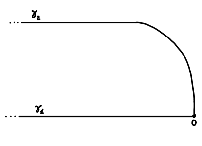
Figure 1.

Consider the Lagrangian submanifolds $\gamma_{1}\times L_{1},\gamma_{2}\times L_{2}\subset\mathbb{R}^{2}\times M$. The surgery construction from [BC6] produces a Lagrangian cobordism $V\subset\mathbb{R}\times M$ with two negative ends which coincide with negative ends of $\gamma_{i}\times L_{i}$ and with whose positive end looks like the positive end of $\gamma_{3}\times(L_{1}\#L_{2})$, where the curve $\gamma_{3}$ is depicted in Figure 2 and $L_{1}\#L_{2}$ stands for the Polterovich surgery (in $M$) of $L_{1}$ and $L_{2}$ (which coincides with the connected sum of the $L_{i}$’s because they intersect transversely at exactly one point). The projection of $V$ to $\mathbb{R}^{2}$ is depicted in Figure 2.

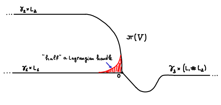
Figure 2.

Next we determine the topology of $V$. Consider the curves $\widetilde{\gamma}_{1},\widetilde{\gamma}_{2}$ (which are extensions of the $\gamma_{i}$’s to curves with positive ends as in Figure 3.)

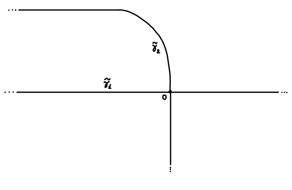
Figure 3.

Consider the Polterovich surgery $W=(\widetilde{\gamma}_{1}\times L_{1})\#(\widetilde{\gamma}_{2}\times L_{2})\subset\mathbb{R}^{2}\times M$ (note that the latter two Lagrangians also intersect transversely at a single point). See Figure 4.

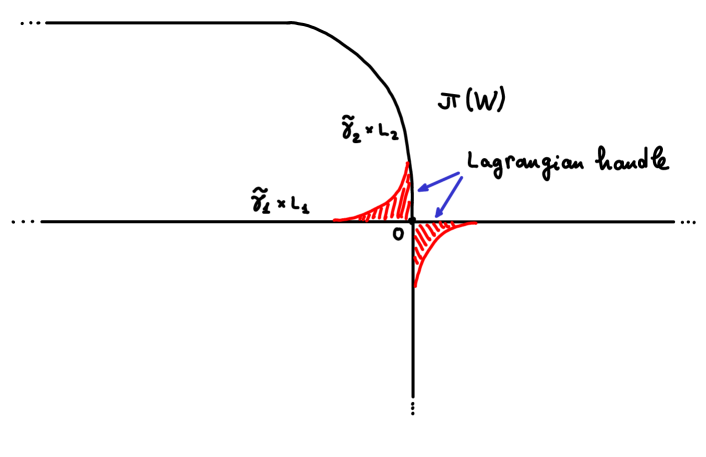
Figure 4.

Figure 5.

Denote by $\pi:\mathbb{R}^{2}\times M\longrightarrow\mathbb{R}^{2}$ the projection, and by $S\subset\mathbb{R}^{2}$ the strip depicted in Figure 5. Put $V_{0}=W\cap\pi^{-1}(S)$. According to [BC6], $V_{0}$ is a manifold with boundary, with two obvious boundary components corresponding to the $L_{i}$’s and a third boundary component which is $W\cap\pi^{-1}(0)$. The latter is exactly the Polterovich surgery $L_{1}\#L_{2}$. Moreover $V_{0}$ is homotopy equivalent to $V$ (in fact $V_{0}\subset V$ and is a deformation retract of $V$). A straightforward calculation shows that there is an embedding $L_{1}\vee L_{2}\subset V_{0}$ and moreover that $L_{1}\vee L_{2}$ is a deformation retract of $V_{0}$. (In fact, one can show that $V_{0}$ is diffeomorphic to the boundary connected sum of $[0,1]\times L_{1}$ and $[0,1]\times L_{2}$, where the connected sum occurs among the boundary components $\{1\}\times L_{i}$, $i=1,2$.)

The statement on monotonicity follows from the Seifert - Van Kampen theorem (see also [BC6]).

Assume now that $L_{1},L_{2}$ are spin. Then $\widetilde{\gamma}_{1}\times L_{1}$ and $\widetilde{\gamma}_{2}\times L_{2}$ are also spin, with a spin structure extending those of the ends. Recall that the connected sum of spin manifolds is also spin [LM3]. Thus $W=(\widetilde{\gamma}_{1}\times L_{1})\#(\widetilde{\gamma}_{2}\times L_{2})$ is spin too and by standard arguments it follows that the spin structure on $W$ can be chosen so that it extends those given on the ends. By restriction we obtain a spin structure on $V_{0}\subset W$ and consequently also the desired one on $V$. ∎

5. Examples

This section is a continuation of §1.3 in which we provide more details to the examples. We will work here with the following setting. $(M,\omega)$ will be a monotone symplectic manifold with minimal Chern number $C_{M}$. To keep the notation short we will denote here by $QH(M)$ the quantum homology of $M$ with coefficients in the ring $R=\mathbb{Z}[q^{-1},q]$ (with $|q|=-2$), instead of writing $QH(M;R)$.

5.1. Lagrangian spheres in symplectic blow-ups of $\mathbb{C}P^{2}$

Denote as in §1.3.1 by $M_{k}$ the blow-up of ${\mathbb{C}}P^{2}$ at $k\leq 6$ points endowed with a Kähler symplectic structure $\omega_{k}$ in the cohomology class of $c_{1}\in H^{2}(M_{k})$. Note that $-K_{M_{k}}$ is ample hence $c_{1}$ represents a Kähler class. Note that $C_{M_{k}}=1$. As will be seen in §8 some of our results (e.g. Theorem A) continue to hold in dimension $4$ also for non-monotone Lagrangian spheres. In this section however we still stick to the monotone case.

We first claim that the set of classes in $H_{2}(M_{k})$ which are represented by Lagrangian spheres are precisely those that appear in Table 1. This is well known and there are many ways to prove it (see e.g. [Sei, Eva, LW, She2]). For the classes $A=E_{i}-E_{j}\in H_{2}(M_{k})$ when $k=2$ and $k=3$ it is easy to find Lagrangian spheres in the class $A$ by an explicit construction which we outline below (see [Eva] for more details). For $k\geq 4$, as well as $k=3$ with $A=H-E_{1}-E_{2}-E_{3}$, it seems less trivial to perform explicit constructions and one could appeal instead to less transparent methods such as (relative) inflation, as in in [LW, She2] (we will briefly outline this in a special case below). Another approach which works for some of the $k$’s is to realize $M_{k}$ as a fiber in a Lefschetz pencil and obtain the Lagrangian spheres as vanishing cycles (e.g. $M_{6}$ is the cubic surface in ${\mathbb{C}}P^{3}$ and $M_{5}$ is a complete intersection of two quadrics in ${\mathbb{C}}P^{4}$). Yet another approach comes from real algebraic geometry, where one can obtain Lagrangian spheres in some of the $M_{k}$’s as a component of the fixed point set of an anti-symplectic involution. This works for $k=5,6$ and all classes $A$, and for $k=3$ with $A=E_{i}-E_{j}$. See [Kol] for more details. Finally note that for $2\leq k\leq 8$, $k\neq 3$, the group of symplectomorphisms of $M_{k}$ acts transitively on the set of classes that can be represented by Lagrangian spheres [Dem, LW], hence it is enough to construct one Lagrangian sphere in each $M_{k}$. (This also explains why the invariants in Table 1 coincide for different classes within each of the $M_{k}$’s with the exception $k=3$.)

Despite the many ways to establish Lagrangian spheres in the $M_{k}$’s, the shortest (albeit not the most explicit) path to this end is to appeal to the work Li-Wu [LW]. According to [LW] a homology class $A\in H_{2}(M_{k})$ can be represented by a Lagrangian sphere iff it satisfies the following two conditions:

1. $A$ can be represented by a smooth embedded $2$-sphere.

2. $\langle[\omega_{k}],A\rangle=0$.

3. $A\cdot A=-2$.

We remark again that we have assumed that $[\omega_{k}]=c_{1}$ (otherwise one has to assume in addition that $\langle c_{1},A\rangle=0$).

It is straightforward to see that all the classes in Table 1 satisfy conditions (LS-2) and (LS-3) above. As for condition (LS-1), note that if $C^{\prime},C^{\prime\prime}\subset M^{4}$ are two disjoint embedded smooth $2$-spheres in a $4$-manifold $M^{4}$, then by performing the connected sum operation one obtains a new smooth embedded $2$-sphere in the class $[C^{\prime}]+[C^{\prime\prime}]$. From this it follows that any non-trivial class of the form $\sum_{i=1}^{k}\epsilon_{i}E_{i}$ with $\epsilon_{i}\in\{-1,0,1\}$ can be represented by a smooth embedded $2$-sphere. This settles the cases $\pm(E_{i}-E_{j})$. For the other type of classes, note that $H$ and $2H$ can both be represented by smooth embedded $2$-spheres (e.g. a projective line and a conic respectively) hence the same holds also for for classes of the form $\pm(H-E_{i}-E_{j}-E_{l})$ and $\pm(2H-\sum_{i=1}^{6}E_{i})$.

We remark that in fact there are no other classes but the ones in Table 1 that can be represented by Lagrangian spheres in $M_{k}$. This can be proved by elementary means using conditions (LS-2) and (LS-3) above.

5.1.1. Construction of Lagrangian spheres in $M_{2}$ and $M_{3}$

We now outline a more explicit way to construct Lagrangian spheres in some of the $M_{k}$’s (c.f. [Eva]). Consider $Q=\mathbb{C}P^{1}\times\mathbb{C}P^{1}$ endowed with the symplectic form $\omega=2\omega_{\mathbb{C}P^{1}}\oplus 2\omega_{\mathbb{C}P^{1}}$, where $\omega_{\mathbb{C}P^{1}}$ is the standard Kähler form on $\mathbb{C}P^{1}$ normalized so that $\mathbb{C}P^{1}$ has area $1$. Note that the first Chern class of $Q$ satisfies $c_{1}=[\omega]$. The symplectic manifold $Q$ contains a Lagrangian sphere $\overline{\Delta}$ in the class $[\mathbb{C}P^{1}\times\textnormal{pt}]-[\textnormal{pt}\times\mathbb{C}P^{1}]$ (i.e. the class of the anti-diagonal). For example, we can write $\overline{\Delta}$ as the graph of the antipodal map, given in homogeneous coordinates by

$$\mathbb{C}P^{1}\longrightarrow\mathbb{C}P^{1},\qquad[z_{0}:z_{1}]\longmapsto[-\overline{z_{1}}:\overline{z_{0}}].$$

Next, we claim that $Q$ admits a symplectic embedding of two disjoint closed balls $B_{1},B_{2}$ of capacity $1$ whose images are disjoint from $\overline{\Delta}$. This can be easily seen from the toric picture. Indeed the image of the moment map of $Q$ is the square $[0,2]\times[0,2]$ and the image of $\overline{\Delta}$ under that map is given by the anti-diagonal $\{(x,y)\mid x,y\in[0,2],x+y=2\}$. By standard arguments in toric geometry we can symplectically embed in $Q$ a ball $B_{1}$ of capacity $1$ whose image under the moment map is $\{(x,y)\mid x,y\in[0,2],x+y\leq 1\}$. Similarly we can embed another ball $B_{2}$ whose image is $\{(x,y)\mid x,y\in[0,2],x+y\geq 3\}$. Clearly $B_{1}$, $B_{2}$ and $\overline{\Delta}$ are mutually disjoint. Denote by $\widetilde{Q}_{1}$ the blow-up of $Q$ with respect to $B_{1}$ and by $\widetilde{Q}_{2}$ the blow-up of $Q$ with respect to both balls $B_{1}$ and $B_{2}$. It is well known that $\widetilde{Q}_{1}$ is symplectomorphic to $M_{2}$ via a symplectomorphism that sends the class $\overline{\Delta}$ to $E_{1}-E_{2}$. And $\widetilde{Q}_{2}$ is symplectomorphic to $M_{3}$ by a similar symplectomorphism. It follows that $E_{1}-E_{2}$ represents Lagrangian spheres both in $M_{2}$ and in $M_{3}$. Construction of Lagrangian spheres in the other classes of the type $E_{i}-E_{j}$ in $M_{3}$ can be done in a similar way.

Lagrangian spheres in the class $H-E_{1}-E_{2}-E_{3}$ in $M_{3}$

We start with the complex blow-up of ${\mathbb{C}}P^{2}$ at three points that lie on the same projective line. Denote by $E_{i}$ the exceptional divisors over the blown-up points. The result of the blow up is a complex algebraic surface $X$ which contains an embedded holomorphic rational curve $\Sigma$ in the class $H-E_{1}-E_{2}-E_{3}$. Note also that there are three embedded holomorphic curves $C_{i}\subset X$, $i=1,2,3$, in the classes $[C_{i}]=H-E_{i}$. Since $[C_{i}]\cdot[\Sigma]=0$ the curves $C_{i}$ are disjoint from $\Sigma$. Pick a Kähler symplectic structure $\omega_{0}$ on $X$. After a suitable normalization we can write $[\omega_{0}]=h-\lambda_{1}e_{1}-\lambda_{2}e_{2}-\lambda_{3}e_{3}$, where $h,e_{1},e_{2},e_{3}$ are the Poincaré duals to $H,E_{1},E_{2},E_{3}$ respectively. It is easy to check that $\lambda_{i}\geq 0$ and that $\lambda_{1}+\lambda_{2}+\lambda_{3}<1$. We now change $\omega_{0}$ to a new symplectic form $\omega^{\prime}$ such that:

1. $\omega^{\prime}$ coincides with $\omega_{0}$ outside a small neighborhood $\mathcal{U}$ of $\Sigma$, where $\mathcal{U}$ is disjoint from the curves $C_{1},C_{2},C_{3}$.

2. $\omega^{\prime}|_{T(\Sigma)}\equiv 0$, i.e. $\Sigma$ becomes a Lagrangian sphere with respect to $\omega^{\prime}$.

3. $\omega^{\prime}$ and $\omega$ are in the same deformation class of symplectic forms on $X$ (i.e. they can be connected by a path of symplectic forms).

This can be achieved for example using the deflation procedure [She2] (see also [LU]). Alternatively, one can construct $\omega^{\prime}$ using Gompf fiber-sum surgery [Gom] with respect to $\Sigma\subset X$ and the diagonal in $\mathbb{C}P^{1}\times\mathbb{C}P^{1}$:

$$(Y,\omega^{\prime\prime})=(X,\omega_{0})\,_{\Sigma}\#_{\textnormal{diag}}\,(\mathbb{C}P^{1}\times\mathbb{C}P^{1},a\omega_{\mathbb{C}P^{1}}\oplus a\omega_{\mathbb{C}P^{1}}),$$

where $a=\tfrac{1}{2}\int_{\Sigma}\omega_{0}$, and $S^{2}$ is symplectically embedded in $X$ as $\Sigma$ and in $\mathbb{C}P^{1}\times\mathbb{C}P^{1}$ as the diagonal. Since the anti-diagonal $\overline{\Delta}$ is a Lagrangian sphere in $\mathbb{C}P^{1}\times\mathbb{C}P^{1}$ which is disjoint from the diagonal it gives rise to a Lagrangian sphere $L^{\prime\prime}\subset Y$. Finally observe that the surgery has not changed the diffeomorphism type of $X$, namely there exists a diffeomorphism $\phi:Y\longrightarrow X$ and moreover $\phi$ can be chosen in such a way that $\phi(L^{\prime\prime})=\Sigma$. Take now $\omega^{\prime}=\phi_{*}\omega^{\prime\prime}$. To obtain a symplectic deformation between $\omega^{\prime}$ and $\omega_{0}$ one can perform the preceding surgery in a suitable one-parametric family, where the symplectic form on $\mathbb{C}P^{1}\times\mathbb{C}P^{1}$ is rescaled so that the area of one of the factors becomes smaller and smaller and the area of the other increases so that the area of the diagonal stays constant.

Having replaced the form $\omega_{0}$ by $\omega^{\prime}$ we have a Lagrangian sphere in the desired homology class $H-E_{1}-E_{2}-E_{3}$ but the form $\omega^{\prime}$ might not be in the cohomology class of $c_{1}$. We will now correct that using inflation.

After a normalization we can assume that $[\omega^{\prime}]=h-\lambda^{\prime}_{1}e_{1}-\lambda^{\prime}_{2}e_{2}-\lambda^{\prime}_{3}e_{3}$. Since $\Sigma$ is Lagrangian with respect to $\omega^{\prime}$ we have $\lambda^{\prime}_{1}+\lambda^{\prime}_{2}+\lambda^{\prime}_{3}=1$. Recall also that the surfaces $C_{1},C_{2},C_{3}$ are symplectic with respect to $\omega^{\prime}$, hence $\lambda^{\prime}_{i}<1$ for every $i$. Moreover, by construction, the surfaces $C_{1},C_{2},C_{3}$ can be made simultaneously $J$-holomorphic for some $\omega^{\prime}$-compatible almost complex structure $J$. Since the $C_{i}$’s are disjoint from $\Sigma$ we can find neighborhoods $U_{i}$ of $C_{i}$ such that the $U_{i}$’s are disjoint from $\Sigma$. We now perform inflation simultaneously along the three surfaces $C_{1},C_{2},C_{3}$. More specifically, by the results of [Bir2, Bir1] there exist closed $2$-forms $\rho_{i}$ supported in $U_{i}$, representing the Poincaré dual of $[C_{i}]$ (i.e. $[\rho_{i}]=h-e_{i}$) and such that the $2$-form

$$\omega_{t_{1},t_{2},t_{3}}=\omega^{\prime}+t_{1}\rho_{1}+t_{2}\rho_{2}+t_{3}\rho_{3}$$

is symplectic for every $t_{1},t_{2},t_{3}\geq 0$. See Lemma 2.1 in [Bir2] and Proposition 4.3 in [Bir1] (see also [Lal, LM1, LM2, McD, MO].) The cohomology class of $\omega^{\prime}_{t}$ is:

$$[\omega^{\prime}_{t}]=(1+t_{1}+t_{2}+t_{3})h-(\lambda^{\prime}_{1}+t_{1})e_{1}-(\lambda^{\prime}_{2}+t_{2})e_{2}-(\lambda^{\prime}_{3}+t_{3})e_{3}.$$

Choosing $t^{0}_{i}=1-\lambda^{\prime}_{i}$ we have $t^{0}_{i}>0$ and $1+t_{1}^{0}+t_{2}^{0}+t_{3}^{0}=4-(\lambda^{\prime}_{1}+\lambda^{\prime}_{2}+\lambda^{\prime}_{3})=3$, hence:

$$[\omega^{\prime}_{t^{0}_{1},t_{2}^{0},t_{3}^{0}}]=3h-e_{1}-e_{2}-e_{3}=c_{1}.$$

Due to the support of the forms $\rho_{i}$ the surface $\Sigma$ remains Lagrangian for $\omega^{\prime}_{t^{0}_{1},t^{0}_{2},t^{0}_{3}}$. Finally note that $\omega^{\prime}_{t^{0}_{1},t^{0}_{2},t^{0}_{3}}$ is in the same symplectic deformation class of $\omega_{0}$ hence by standard results $(X,\omega^{\prime}_{t^{0}_{1},t^{0}_{2},t^{0}_{3}})$ is symplectomorphic to $M_{3}$.

5.1.2. Calculation of the discriminant for $M_{k}$, $2\leq k\leq 6$

We now give more details on the calculation of the discriminant $\Delta_{L}$ for each of the examples in Table 1. In what follows, for a symplectic manifold $M$, we denote by $p\in H_{0}(M)$ the homology class of a point. As before we write $QH(M)$ for the quantum homology ring of $M$ with coefficients in $R=\mathbb{Z}[q^{-1},q]$ where $|q|=-2$. The calculations below make use of the “multiplication table” of the quantum homology of the $M_{k}$’s which can be found in [CM].

Recall that for $M_{k}$ with $4\leq k\leq 6$ the group of symplectomorphisms of $M_{k}$ acts transitively on the set of classes that can be represented by Lagrangian spheres [Dem, LW]. Therefore, for $k\geq 4$ we will perform explicit calculations only for Lagrangians in the class $E_{1}-E_{2}$.

Before we go on we remark that all the calculations for the $M_{k}$’s below extend without any change in case we endow $M_{k}$ with a non-monotone symplectic structure (provided that a Lagrangian sphere in the respective class still exists). This is special to dimension $4$ and is explained in detail in §8.

5.1.3. 2-point blow-up of $\mathbb{C}P^{2}$

$QH(M_{2})$ has the following ring structure:

$$p*p=Hq^{3}+[M_{2}]q^{4}$$

$$p*H=(H-E_{1})q^{2}+(H-E_{2})q^{2}+[M_{2}]q^{3}$$

$$p*E_{i}=(H-E_{i})q^{2}$$

$$H*H=p+(H-E_{1}-E_{2})q+2[M_{2}]q^{2}$$

$$H*E_{i}=(H-E_{1}-E_{2})q+[M_{2}]q^{2}$$

$$E_{1}*E_{2}=(H-E_{1}-E_{2})q$$

$$E_{1}*E_{1}=-p+(H-E_{2})q+[M_{2}]q^{2}$$

$$E_{2}*E_{2}=-p+(H-E_{1})q+[M_{2}]q^{2}.$$

Consider Lagrangian spheres $L\subset M_{2}$ in the class $E_{1}-E_{2}$. A straightforward calculation shows that:

$$(E_{1}-E_{2})^{*3}-5(E_{1}-E_{2})q^{2}=0,$$

and thus we obtain $\Delta_{L}=5$. Multiplication of $c_{1}$ with $[L]$ gives: $c_{1}*(E_{1}-E_{2})=(-1)(E_{1}-E_{2})q$, hence $\lambda_{L}=-1$. The associated ideal (see §2.4) $\mathcal{I}_{L}\subset QH_{*}(M_{2})$ is:

$$\mathcal{I}(E_{1}-E_{2})=R(-2p+(E_{1}+E_{2})q+2[M_{2}]q^{2})\oplus R(E_{1}-E_{2}).$$

We now turn to Theorem 3.A and calculate explicitly the coefficients $\sigma_{c,L}$, $\tau_{c,L}$ from equation (11). Consider a general element $c=dH-m_{1}E_{1}-m_{2}E_{2}\in H_{2}(M_{2})$, where $d,m_{1},m_{2}\in\mathbb{Z}$. Then $\xi:=c\cdot[L]=m_{1}-m_{2}$ and we assume that $m_{1}\neq m_{2}$. A straightforward calculation gives:

$$\sigma_{c,L}=-\frac{m_{1}+m_{2}}{m_{1}-m_{2}},\quad\tau_{c,L}=\frac{m_{1}^{2}-3m_{1}m_{2}+m_{2}^{2}}{(m_{1}-m_{2})^{2}}.$$

One can easily check that $\sigma_{c,L}^{2}+4\tau_{c,L}=5$.

5.1.4. 3-point blow-up of $\mathbb{C}P^{2}$

$QH(M_{3})$ has the following ring structure:

$$p*p=(3H-E_{1}-E_{2}-E_{3})q^{3}+3[M_{3}]q^{4}$$

$$p*H=(3H-E_{1}-E_{2}-E_{3})q^{2}+3[M_{3}]q^{3}$$

$$p*E_{i}=(H-E_{i})q^{2}+[M_{3}]q^{3}$$

$$H*H=p+(3H-2E_{1}-2E_{2}-2E_{3})q+3[M_{3}]q^{2}$$

$$H*E_{i}=(2H-2E_{i}-E_{j}-E_{k})q+[M_{3}]q^{2},\quad i\neq j\neq k\neq i$$

$$E_{i}*E_{i}=-p+(2H-E_{1}-E_{2}-E_{3})q+[M_{3}]q^{2}$$

$$E_{i}*E_{j}=(H-E_{i}-E_{j})q,\quad i\neq j.$$

Consider Lagrangians $L,L^{\prime}\subset M_{3}$ in the classes $[L]=E_{i}-E_{j}$ and $[L^{\prime}]=H-E_{1}-E_{2}-E_{3}$. The corresponding Lagrangian cubic equations are given by:

$$(E_{i}-E_{j})^{*3}-4(E_{i}-E_{j})q^{2}=0,$$

$$(H-E_{1}-E_{2}-E_{3})^{*3}+3(H-E_{1}-E_{2}-E_{3})q^{2}=0,$$

and thus obtain $\Delta_{L}=4$ and $\Delta_{L^{\prime}}=-3$. Multiplication with $c_{1}$ gives:

$$c_{1}*(E_{i}-E_{j})=(-2)(E_{i}-E_{j})t,$$

$$c_{1}*(H-E_{1}-E_{2}-E_{3})=(-3)(H-E_{1}-E_{2}-E_{3})t,$$

hence $\lambda_{L}=-2$ and $\lambda_{L^{\prime}}=-3$. The associated ideals in $QH(M_{3})$ are:

$$\mathcal{I}_{L}=R(-2p+2(H-E_{3})t+2[M_{3}]q^{2})\oplus R(E_{1}-E_{2}),$$

$$\mathcal{I}_{L^{\prime}}=R(-2p+(3H-E_{1}-E_{2}-E_{3})q+4[M_{3}]q^{2})\oplus R(H-E_{1}-E_{2}-E_{3}).$$

The Lagrangian spheres in different homology classes of the type $E_{i}-E_{j}$ in $M_{3}$ have the same discriminant and the same eigenvalue $\lambda_{L}$. This is so because for every $i<j$ there is a symplectomorphism $\varphi:M_{3}\longrightarrow M_{3}$ such that $\varphi_{*}(E_{1}-E_{2})=E_{i}-E_{j}$. In contrast, note that there exists no symplectomorphism of $M_{3}$ sending $E_{1}-E_{2}$ to $H-E_{1}-E_{2}-E_{3}$.

5.1.5. 4-point blow-up of $\mathbb{C}P^{2}$

$QH(M_{4})$ has the following ring structure:

$$p*p=(9H-3E_{1}-3E_{2}-3E_{3}-3E_{4})q^{3}+10[M_{4}]q^{4}$$

$$p*H=(8H-3E_{1}-3E_{2}-3E_{3}-3E_{4})q^{2}+9[M_{4}]q^{3}$$

$$p*E_{i}=(3H-2E_{i}-\sum\limits_{j\neq i}E_{j})q^{2}+3[M_{4}]q^{3}$$

$$H*H=p+(6H-3E_{1}-3E_{2}-3E_{3}-3E_{4})q+8[M_{4}]q^{2}$$

$$H*E_{i}=(3H-3E_{i}-\sum\limits_{j\neq i}E_{j})q+3[M_{4}]q^{2}$$

$$E_{i}*E_{i}=-p+(3H-2E_{i}-\sum\limits_{j\neq i}E_{j})q+2[M_{4}]q^{2}$$

$$E_{i}*E_{j}=(H-E_{i}-E_{j})q+[M_{4}]q^{2}$$

As explained above it is enough to calculate our invariants for Lagrangians in the class $E_{1}-E_{2}$. A straightforward calculation shows that:

$$(E_{1}-E_{2})^{*3}=(E_{1}-E_{2})q^{2},\quad c_{1}*(E_{1}-E_{2})=-3(E_{1}-E_{2})q,$$

hence $\Delta_{L}=1$ and $\lambda_{L}=-3$. The associated ideals for Lagrangians $L$, $L^{\prime}$ with $[L]=E_{1}-E_{2}$ and $L^{\prime}=H-E_{1}-E_{2}-E_{3}$ are:

$$\mathcal{I}_{L}=R(-2p+(4H-E_{1}-E_{2}-2E_{3}-2E_{4})q+2[M_{4}]q^{2})\oplus R(E_{1}-E_{2}),$$

$$\mathcal{I}_{L^{\prime}}=R(-2p+(3H-E_{1}-E_{2}-E_{3})q+2[M_{4}]q^{2})\oplus R(H-E_{1}-E_{2}-E_{3}).$$

5.1.6. 5-point blow-up of $\mathbb{C}P^{2}$

$QH(M_{5})$ has the following ring structure:

$$p*p=(36H-12E_{1}-12E_{2}-12E_{3}-12E_{4}-12E_{5})q^{3}+52[M_{5}]q^{4}$$

$$p*H=(25H-9E_{1}-9E_{2}-9E_{3}-9E_{4}-9E_{5})q^{2}+36[M_{5}]q^{3}$$

$$p*E_{i}=(9H-5E_{i}-3\sum\limits_{j\neq i}E_{j})q^{2}+12[M_{5}]q^{3}$$

$$H*H=p+(18H-8E_{1}-8E_{2}-8E_{3}-8E_{4}-8E_{5})q+25[M_{5}]q^{2}$$

$$H*E_{i}=(8H-6E_{i}-3\sum\limits_{j\neq i}E_{j})q+9[M_{5}]q^{2}$$

$$E_{i}*E_{i}=-p+(6H-4E_{i}-2\sum\limits_{j\neq i}E_{j})q+5[M_{5}]q^{2}$$

$$E_{i}*E_{j}=(3H-2E_{i}-2E_{j}-\sum\limits_{k\neq i,j}E_{k})q+3[M_{5}]q^{2}$$

As before, it is enough to consider only the case $[L]=E_{1}-E_{2}$. A direct calculation gives:

$$(E_{1}-E_{2})^{*3}=0,\quad c_{1}*(E_{1}-E_{2})=-4(E_{1}-E_{2})q,$$

hence $\Delta_{L}=0$, $\lambda_{L}=-4$.

The associated ideals for Lagrangians $L$, $L^{\prime}$ with $[L]=E_{1}-E_{2}$ and $[L^{\prime}]=H-E_{1}-E_{2}-E_{3}$ are:

$$\mathcal{I}_{L}=R(-2p+(6H-2E_{1}-2E_{2}-2E_{3}-2E_{4}-2E_{5})q+4[M_{5}]q^{2})\oplus R(E_{1}-E_{2}),$$

$$\mathcal{I}_{L^{\prime}}=R(-2p+(6H-2E_{1}-2E_{2}-2E_{3}-2E_{4}-2E_{5})q+4[M_{5}]q^{2})\oplus R(H-E_{1}-E_{2}-E_{3}).$$

5.1.7. 6-point blow-up of $\mathbb{C}P^{2}$

$QH(M_{6})$ has the following the ring structure:

$$p*p=(252H-84E_{1}-84E_{2}-84E_{3}-84E_{4}-84E_{5}-84E_{6})q^{3}+540[M_{6}]q^{4}$$

$$p*H=(120H-42E_{1}-42E_{2}-42E_{3}-42E_{4}-42E_{5}-42E_{6})q^{2}+252[M_{6}]q^{3}$$

$$p*E_{i}=(42H-20E_{i}-14\sum\limits_{j\neq i}E_{j})q^{2}+84[M_{6}]q^{3}$$

$$H*H=p+(63H-25E_{1}-25E_{2}-25E_{3}-25E_{4}-25E_{5}-25E_{6})q+120[M_{6}]q^{2}$$

$$H*E_{i}=(25H-15E_{i}-9\sum\limits_{j\neq i}E_{j})q+42[M_{6}]q^{2}$$

$$E_{i}*E_{i}=-p+(15H-9E_{i}-5\sum\limits_{j\neq i}E_{j})q+20[M_{6}]q^{2}$$

$$E_{i}*E_{j}=(9H-5E_{i}-5E_{j}-3\sum\limits_{k\neq i,j}E_{j})q+14[M_{6}]q^{2}$$

Again, we may assume without loss of generality that $[L]=E_{1}-E_{2}$. A direct calculation gives:

$$(E_{1}-E_{2})^{*3}=0,\quad c_{1}*(E_{1}-E_{2})=-6(E_{1}-E_{2})q,$$

hence $\Delta_{L}=0$, $\lambda_{L}=-6$.

Interestingly, the associated ideals $\mathcal{I}_{L}$ for Lagrangians $L$ in any of the classes: $E_{i}-E_{j}$, $2H-E_{i}-E_{j}-E_{l}$, $2H-E_{1}-E_{2}-E_{3}-E_{4}-E_{5}-E_{6}$ all coincide:

$$\mathcal{I}_{L}=R(-2p+(12H-4\sum_{j=1}^{6}E_{j})q+12[M_{6}]q^{2})\bigoplus R(2H-\sum_{j=1}^{6}E_{j}).$$

Remark 5.1.A.

Note that all Lagrangian spheres in each of $M_{4}$, $M_{5}$ and $M_{6}$ have the same discriminant and the same holds for the Lagrangian spheres in $M_{3}$ in the classes $E_{1}-E_{2}$, $E_{2}-E_{3}$ and $E_{1}-E_{3}$. This follows of course from the fact that all these classes belong to the same orbit of the action of the symplectomorphism group (on each of the $M_{k}$’s). However, here is a different potential explanation which might give more insight. Consider for example the classes $E_{1}-E_{2}$ and $E_{2}-E_{3}$ in $M_{3}$. It seems reasonable to expect that there exist Lagrangian spheres $L_{1},L_{2}\subset M_{3}$ with $[L_{1}]=E_{1}-E_{2}$, $[L_{2}]=E_{2}-E_{3}$ such that $L_{1}$ and $L_{2}$ intersect transversely at exactly one point. (We have not verified the details of that, but this seems plausible in view of the constructions outlined at the beginning of §5.1.1). The fact that $\Delta_{L_{1}}=\Delta_{L_{2}}$ would now follow from Corollary F. Similar arguments should apply to many other pairs of classes on $M_{4}$, $M_{5}$ and $M_{6}$. This would also explain why in all these cases the discriminants turn out to be perfect squares.

5.2. Lagrangian spheres in hypersurfaces of ${\mathbb{C}}P^{n+1}$

Let $M^{2n}\subset\mathbb{C}P^{n+1}$ be a Fano hypersurface of degree $d$, where $n\geq 3$. We endow $M$ with the symplectic structure induced from ${\mathbb{C}}P^{n+1}$. It is easy to check that $M$ is monotone and that the minimal Chern number is $C_{M}=n+2-d$.

We view the homology $H_{*}(M;\mathbb{Q})$ as a ring, endowed with the intersection product which we denote by $a\cdot b$ for $a,b\in H_{*}(M;\mathbb{Q})$. Write $h\in H_{2n-2}(M;\mathbb{Q})$ for the class of a hyperplane section. The homology $H_{*}(M;\mathbb{Q})$ is generated as a ring by the class $h$ and the subspace of primitive classes, denoted by $H_{n}(M;\mathbb{Q})_{0}$. (Recall that the latter is by definition the kernel of the map $H_{n}(M;\mathbb{Q})\longrightarrow H_{n-2}(M;\mathbb{Q})$, $a\longmapsto a\cdot h$).

Assume that $d\geq 2$. Then by Picard-Lefschetz theory $M$ contains Lagrangian spheres (that can be realized as vanishing cycles of the Lefschetz pencil associated to the embedding $M\subset{\mathbb{C}}P^{n+1}$).

Let $L\subset M$ be a Lagrangian sphere and assume further that $d\geq 3$. To calculate $[L]^{*3}$ we appeal to the work of Collino-Jinzenji [CJ] (see also [Giv, Bea, Tia] for related results). We set $x:=h+d![M]q$ if $C_{M}=1$, and $x:=h$, if $C_{M}\geq 2$. Specifically, we will need the following:

Theorem 5.2.A (Collino-Jinzenji [CJ]).

In the quantum homology ring of $M$ with coefficients in $\mathbb{Q}[q]$ we have the following identities:

1. $x*a=0$ for every $a\in H_{n}(M;\mathbb{Q})_{0}$.

2. $a*b=\frac{1}{d}\#(a\cdot b)(x^{*n}-d^{d}x^{*(d-2)}q^{n+2-d})$ for every $a,b\in H_{n}(M;\mathbb{Q})_{0}$.

Coming back to our Lagrangian spheres $L\subset M$, we clearly have $[L]\in H_{n}(M;\mathbb{Q})_{0}$. Therefore we obtain from Theorem 5.2.A:

(30) $$[L]*[L]*[L]=\frac{1}{d}\#([L]\cdot[L])(x^{*n}*[L]-d^{d}x^{*(d-2)}*[L]q^{n+2-d})=0,$$

where in the last equality we have used that $d>2$ (hence $x^{*(d-2)}*[L]=0$).

If we also assume that $2C_{M}|n$, then the Lagrangian spheres $L\subset M$ have minimal Maslov number $N_{L}=2C_{M}$ and it is easy to see that they satisfy Assumption $\mathscr{L}$ (see e.g. Proposition G). Therefore in this case the discriminant $\Delta_{L}$ is defined and we clearly have $\Delta_{L}=0$. (Note that when $2C_{M}|n$ we must have $d>2$.)

Finally, we discuss the case $d=2$. A straightforward calculation based on the quantum homology ring structure of the quadric (see e.g. [Bea]) shows that Lagrangian spheres $L\subset M$ satisfy $[L]^{*3}=(-1)^{\frac{n(n-1)}{2}+1}4[L]q^{n}$ if $n=$ even and $[L]=0$ (hence $[L]^{*2}=0$) if $n=$ odd.

5.2.1. An example which is not a sphere

All our examples so far were for Lagrangians that are spheres. However, our theory is more general and applies to other topological types of Lagrangians (see e.g. Assumption $\mathscr{L}$, Proposition G and Theorem B). Here is such an example with $L\approx S^{m}\times S^{m}$.

Let $Q\subset\mathbb{C}P^{m+1}$ be the complex $n$-dimensional quadric $Q=\{[z_{0}:\ldots:z_{m+1}]\,|\,-z_{0}^{2}+\ldots+z_{m+1}^{2}=0\}$ endowed with the symplectic structure induced from ${\mathbb{C}}P^{m+1}$. Then $S:=\{[z_{0}:\ldots:z_{m+1}]\,|\,-z_{0}^{2}+\ldots+z_{m+1}^{2}=0,z_{i}\in\mathbb{R}\}$ is a Lagrangian sphere. The first Chern class $c_{1}$ of $Q$ equals the Poincaré dual of $mh$, where $h$ is a hyperplane section of $Q$ associated to the projective embedding $Q\subset{\mathbb{C}}P^{m+1}$. The minimal Chern number is $C_{Q}=m$ and $S$ has minimal Maslov number $N_{S}=2m$. Note that $S$ does not satisfy Assumption $\mathscr{L}$ (since $N_{S}$ does not divide $m$). Henceforth we will assume that $m=$ even.

Put $M=Q\times Q$ endowed with the split symplectic structure induced from both factors and consider the Lagrangian submanifold $L\subset M$ which is the product of two copies of $S$:

$$L:=S\times S\subset Q\times Q.$$

Put $2n=\dim_{\mathbb{R}}M$ so that $\dim L=n=2m$.

The symplectic manifold $Q\times Q$ has minimal Chern number $C_{M}=m$ and the minimal Maslov number of $L$ is $N_{L}=2m=n$. By Proposition G, $L$ satisfies Assumption $\mathscr{L}$.

For our calculations the following identities in the quantum homology ring of $Q$ will be relevant (see e.g. [Bea]):

1. $h*[S]=0$.

2. $a*b=\frac{1}{2}\#(a\cdot b)(h^{*m}-4[Q]q^{m})$ for every $a,b\in H_{m}(Q;\mathbb{Q})_{0}$.

To calculate $\Delta_{L}$ we compute $[L]^{*3}$ in $QH(Q\times Q)$. By the Künneth formula in quantum homology [MS] we have $QH(Q\times Q;\mathbb{Z}[q])\cong QH(Q;\mathbb{Z}[q])\otimes_{\mathbb{Z}[q]}QH(Q;\mathbb{Z}[q])$. Together with the previous identities (with $a=b=[S]$) this gives:

$$[L]*[L]=([S]*[S])\otimes([S]*[S])=(h^{*m}-4[Q]q^{m})\otimes(h^{*m}-4[Q]q^{m}),$$

and therefore

$$[L]^{*3}=(h^{*m}*[S]-4[S]q^{m})\otimes(h^{*m}*[S]-4[S]q^{m})=16[S]\otimes[S]q^{2m}=16[L]q^{2m}.$$

It follows that $\sigma_{L}=0$ and $\tau_{L}=1$ (in the notation of Theorem B), hence $\Delta_{L}=4\tau_{L}=4$.

6. Finer invariants over the positive group ring

Much of the theory developed in the previous sections can be enriched so that the discriminant $\Delta_{L}$ and the cubic equation take into account the homology classes of the holomorphic curves involved in their definition. The result is clearly a finer invariant.

We now briefly explain this generalization. Let $L\subset(M,\omega)$ be a monotone Lagrangian submanifold. Denote by $H_{2}^{D}(M,L)\subset H_{2}(M,L;\mathbb{Z})$ the image of the Hurewicz homomorphism $\pi_{2}(M,L)\longrightarrow H_{2}(M,L;\mathbb{Z})$. We abbreviate $H_{2}^{D}=H_{2}^{D}(M,L)$ when $L$ is clear from the discussion.

We will use here the ring $\widetilde{\Lambda}^{+}$, introduced in [BC4], which is the most general ring of coefficients for Lagrangian quantum homology. It can be viewed as a positive version (with respect to $\mu$) of the group ring over $H_{2}^{D}$. Specifically, denote by $\widetilde{\Lambda}^{+}$ the following ring:

(31) $$\widetilde{\Lambda}^{+}=\biggl{\{}p(T)\mid p(T)=c_{0}+\sum_{\begin{subarray}{c}A\in H_{2}^{D}\\ \mu(A)>0\end{subarray}}c_{A}T^{A},\quad c_{0},c_{A}\in\mathbb{Z}\biggr{\}}.$$

We grade $\widetilde{\Lambda}^{+}$ by assigning to the monomial $T^{A}$ degree $|T^{A}|=-\mu(A)$. Note that the degree-$0$ component of $\widetilde{\Lambda}^{+}$ is just $\mathbb{Z}$ (not linear combinations of $T^{A}$ with $\mu(A)=0$). As explained in [BC4] we can define $QH(L;\widetilde{\Lambda}^{+})$, and in fact $QH(L;\mathcal{R})$ for rings $\mathcal{R}$ which are $\widetilde{\Lambda}^{+}$-algebras.

Similarly to $\widetilde{\Lambda}^{+}$ we associate to the ambient manifold the ring $\widetilde{\Gamma}^{+}$. This ring is defined in the same way as $\widetilde{\Lambda}^{+}$ but with $H_{2}^{D}$ replaced by $H_{2}^{S}:=\textnormal{image\,}(\pi_{2}(M)\longrightarrow H_{2}(M;\mathbb{Z}))$ and with $\mu(A)>0$ replaced by $\langle c_{1},A\rangle>0$ in (31). To avoid confusion we will denote the formal variable in $\widetilde{\Gamma}^{+}$ with $S$ and we grade $|S^{A}|=-2\langle c_{1},A\rangle$. Similarly to $QH(L;\widetilde{\Lambda}^{+})$ we can define the ambient quantum homology $QH(M;\widetilde{\Gamma}^{+})$ with coefficients in $\widetilde{\Gamma}^{+}$ and in fact with coefficients in any ring $\mathcal{A}$ which is a $\widetilde{\Gamma}^{+}$-algebra. In particular, since the map $H_{2}^{S}\longrightarrow H_{2}^{D}$ gives $\widetilde{\Lambda}^{+}$ the structure of an $\widetilde{\Gamma}^{+}$-algebra and we can define $QH(M;\widetilde{\Lambda}^{+})=QH(M;\widetilde{\Gamma}^{+})\otimes_{\widetilde{\Gamma}^{+}}\widetilde{\Lambda}^{+}$.

Assume for simplicity that $L$ satisfies the assumptions of Proposition G. Then the conclusion of Proposition G holds with $HF(L,L)$ replaced by $QH(L;\widetilde{\Lambda}^{+})$ in the sense that $\textnormal{rank}_{\mathbb{Z}}\,QH_{0}(L;\widetilde{\Lambda}^{+})/\widetilde{\Lambda}^{+}_{-n}e_{L}=1$, where $\widetilde{\Lambda}^{+}_{-n}\subset\widetilde{\Lambda}^{+}$ stands for the subgroup generated by the homogeneous elements of degree $-n$. Assume further that $L$ is oriented and spinable. Again, the main example satisfying all these assumptions is $L$ being a Lagrangian sphere in a monotone symplectic manifold $M$ with $2C_{M}|\dim L$.

The definition of the discriminant $\Delta_{L}$ carries over to this setting as follows. Pick an element $x\in QH_{0}(L;\widetilde{\Lambda}^{+})$ which lifts $[\textnormal{point}]\in H_{0}(L)$ as in §2.5.4. Write

$$x*x=\widetilde{\sigma}x+\widetilde{\tau}e_{L},$$

where $\widetilde{\sigma},\widetilde{\tau}\in\widetilde{\Lambda}^{+}$ are elements of degrees $|\widetilde{\sigma}|=-n$ and $|\widetilde{\tau}|=-2n$ respectively. As before, the elements $\widetilde{\sigma}$ and $\widetilde{\tau}$ depend on $x$. Define

$$\widetilde{\Delta}_{L}=\widetilde{\sigma}^{2}+4\widetilde{\tau}\in\widetilde{\Lambda}^{+}.$$

The same arguments as in §2.5 show that $\widetilde{\Delta}_{L}$ is independent of the choice of $x$.

Theorems A, B continue to hold but the cubic equation (1) now has the form:

(32) $$[L]^{*3}-\varepsilon\chi\widetilde{\sigma}_{L}[L]^{*2}-\chi^{2}\widetilde{\tau}_{L}[L]=0,$$

where $\widetilde{\sigma}_{L}\in\tfrac{1}{\chi^{2}}\widetilde{\Lambda}^{+}$, $\widetilde{\tau}_{L}\in\tfrac{1}{\chi^{3}}\widetilde{\Lambda}^{+}$ are uniquely determined. (Note that in (32) we do not have the variable $q$ anymore since the elements $\chi^{2}\widetilde{\sigma}_{L},\chi^{3}\widetilde{\tau}_{L}$ are assumed in advance to be in the ring $\widetilde{\Lambda}^{+}$.) As for identity (2), it now becomes:

(33) $$\widetilde{\sigma}_{L}=\frac{1}{\chi^{2}}\sum_{A}GW_{A,3}([L],[L],[L])T^{j(A)},$$

where $j:H_{2}^{S}\longrightarrow H_{2}^{D}$ is the map induced by inclusion.

Analogous versions of Theorem 3.A hold over $\widetilde{\Lambda}^{+}$ too.

Denoting by $\bar{L}$ the Lagrangian $L$ with the opposite orientation, it is easy to check that

(34) $$\widetilde{\sigma}_{\bar{L}}=-\widetilde{\sigma}_{L},\quad\widetilde{\tau}_{\bar{L}}=\widetilde{\tau}_{L},\quad\widetilde{\Delta}_{\bar{L}}=\widetilde{\Delta}_{L}.$$

We now discuss the action of symplectic diffeomorphisms on these invariants. Let $\varphi:M\longrightarrow M$ be a symplectomorphism. The action $\varphi^{M}_{*}:H_{2}^{S}\longrightarrow H_{2}^{S}$ of $\varphi$ on homology induces an isomorphism of rings $\varphi_{\Gamma}:\widetilde{\Gamma}^{+}\longrightarrow\widetilde{\Gamma}^{+}$. Put $L^{\prime}=\varphi(L)$. Instead of the preceding ring $\widetilde{\Lambda}^{+}$ we now have two rings $\widetilde{\Lambda}_{L}^{+}$ and $\widetilde{\Lambda}_{L^{\prime}}^{+}$ associated to $L$ and to $L^{\prime}$ respectively. The action $\varphi^{(M,L)}_{*}:H_{2}^{D}(M,L)\longrightarrow H_{2}^{D}(M,L^{\prime})$ of $\varphi$ on homology induces an isomorphism of rings $\varphi_{\Lambda}:\widetilde{\Lambda}_{L}^{+}\longrightarrow\widetilde{\Lambda}_{L^{\prime}}^{+}$. Moreover, writing an $\mathcal{R}$-algebra $\mathcal{A}$ as ${}_{\mathcal{R}}\mathcal{A}$, the pair of maps $(\varphi_{\Lambda},\varphi_{\Gamma})$ gives rise to an isomorphism of algebras ${}_{\widetilde{\Gamma}^{+}}\widetilde{\Lambda}_{L}^{+}\longrightarrow\,_{\widetilde{\Gamma}^{+}}\widetilde{\Lambda}_{L^{\prime}}^{+}$.

Turning to quantum homologies, standard arguments together with the previous discussion yield two ring isomorphisms (both denoted $\varphi_{Q}$ by abuse of notation):

$$\varphi_{Q}:QH(L;\widetilde{\Lambda}^{+}_{L})\longrightarrow QH(L^{\prime};\widetilde{\Lambda}^{+}_{L^{\prime}}),\quad\varphi_{Q}:QH(M;\widetilde{\Lambda}^{+}_{L})\longrightarrow QH(M;\widetilde{\Lambda}^{+}_{L^{\prime}}),$$

which are linear over $\widetilde{\Gamma}^{+}$ via $\varphi_{\Gamma}$ and also $(\widetilde{\Lambda}_{L}^{+},\widetilde{\Lambda}_{L^{\prime}}^{+})$ linear via $\varphi_{\Lambda}$. Most of the theory from §2.2 extends, with suitable modifications, to the present setting.

The following follows immediately from the preceding discussion and (34) above:

Theorem 6.A.

Let $\varphi:M\longrightarrow M$ be a symplectomorphism. Then:

$$\widetilde{\sigma}_{\varphi(L)}=\varphi_{\Lambda}(\widetilde{\sigma}_{L}),\quad\widetilde{\tau}_{\varphi(L)}=\varphi_{\Lambda}(\widetilde{\tau}_{L}),\quad\widetilde{\Delta}_{\varphi(L)}=\varphi_{\Lambda}(\widetilde{\Delta}_{L}).$$

In particular $\widetilde{\tau}_{L}$ and $\widetilde{\Delta}_{L}$ are invariant under the action of the group $\textnormal{Symp}(M,L)$ of symplectomorphisms $\varphi:(M,L)\longrightarrow(M,L)$ and $\widetilde{\sigma}_{L}$ is invariant under the action of the subgroup $\textnormal{Symp}^{+}(M,L)\subset\textnormal{Symp}(M,L)$ of those $\varphi$’s that preserve the orientation on $L$. If $\varphi\in\textnormal{Symp}(M,L)$ reverses orientation on $L$ then $\varphi_{\Lambda}(\widetilde{\sigma}_{L})=-\widetilde{\sigma}_{L}$.

Next we have the following analogue of Corollary C:

Corollary 6.B.

Let $L\subset M$ be a Lagrangian sphere, where $M$ is a monotone symplectic manifold with $2C_{M}|\dim L$. Then $\widetilde{\sigma}_{L}=0$. In particular, $\widetilde{\Delta}_{L}=4\widetilde{\tau}_{L}$.

Proof.

Denote by $\varphi:M\longrightarrow M$ the Dehn-twist associated to the Lagrangian sphere $L$. Since $n=\dim L=$ even, the restriction $\varphi|_{L}$ reverses orientation on $L$. By Theorem 6.A, $\varphi_{\Lambda}(\widetilde{\sigma}_{L})=-\widetilde{\sigma}_{L}$. Thus the corollary would follow if we show that $\varphi_{\Lambda}=\textnormal{id}$. To show the latter we need to prove that the map induced by $\varphi$ on homology $\varphi^{(M,L)}_{*}:H_{2}(M,L)\longrightarrow H_{2}(M,L)$ is the identity.

Assume first that $n>2$. Then the map induced by inclusion $H_{2}(M)\to H_{2}(M,L)$ is an isomorphism. Moreover, for every $A\in H_{2}(M)$ we can find a a cycle $C$ representing $A$ which lies in the complement of the support of $\varphi$. This shows that $\varphi^{M}_{*}(A)=A$ hence $\varphi^{(M,L)}_{*}=\textnormal{id}$.

Assume now that $n=2$. Then we have $H_{2}(M,L)\cong H_{2}(M)/\mathbb{Z}[L]$. By the Picard-Lefschetz formula, the action of $\varphi^{M}_{*}$ on $H_{2}(M)$ is given by:

$$\varphi^{M}_{*}(A)=A+\#(A\cdot[L])[L].$$

It immediately follows that $\varphi^{(M,L)}_{*}:H_{2}(M,L)\longrightarrow H_{2}(M,L)$ is trivial. ∎

6.1. Other rings of interest

The results in this section continue to hold if we replace the ring $\widetilde{\Lambda}^{+}$ by any $\widetilde{\Lambda}^{+}$-algebra $\mathcal{R}$ (graded or not). See Section 2.1.2 of [BC4] for the precise definitions (in the graded case). Such a structure is defined e.g. by specifying a ring homomorphism $\eta:\widetilde{\Lambda}^{+}\longrightarrow\mathcal{R}$. The most natural examples are:

1. $\mathcal{R}=\mathbb{Z}$, $\mathbb{Q}$ or $\mathbb{C}$, where $\eta(T^{A})=1$.

2. $\mathcal{R}=\mathbb{Z}[t^{-1},t]$, where $\eta(T^{A})=t^{\mu(A)/N_{L}}$.

3. $\mathcal{R}=\mathbb{C}$, with $\eta(T^{A})=\rho(A)$, where $\rho:H_{2}^{D}\longrightarrow\mathbb{C}^{*}$ is a given group homomorphism. This is sometime referred to as twisted coefficients.

4. $\mathcal{R}=\Lambda_{\textnormal{Nov}}$ is the Novikov ring (say in the variable $u$), and $\eta(T^{A})=u^{\omega(A)}$.

5. Combinations of (3) with any of the other possibilities.

6. $\mathcal{R}$ is defined similarly to $\widetilde{\Lambda}^{+}$ but instead of taking powers $T^{A}$ of with $A\in H_{2}^{D}$ we take $A\in H_{2}^{D}/K$, where $K\subset\ker\mu$. See Remark 6.1.A for such an example. (Of course we can take quotients by a subgroup $K\subset H_{2}^{D}$ with $\mu|_{K}\neq 0$. Then we can still define an $\widetilde{\Lambda}^{+}$-algebra $\mathcal{R}$ by taking all linear combinations of $T^{A}$ with $A\in H_{2}^{D}/K$.)

In all cases the Lagrangian cubic equation will hold with coefficients in $\mathcal{R}$ and the coefficients $\sigma^{\mathcal{R}}_{L},\tau^{\mathcal{R}}_{L}$ and discriminant $\Delta^{\mathcal{R}}_{L}$ will now be elements of $\mathcal{R}$. Moreover if $\eta:\widetilde{\Lambda}^{+}\to\mathcal{R}$ is the ring homomorphism defining the $\widetilde{\Lambda}^{+}$-algebra structure on $\mathcal{R}$ then $\eta$ induces ring homomorphisms $QH(L;\widetilde{\Lambda}^{+})\longrightarrow QH(L;\mathcal{R})$ and $\eta_{Q}:QH(M;\widetilde{\Lambda}^{+})\longrightarrow QH(M;\mathcal{R})$. Applying $\eta_{Q}$ to the cubic equation (32) we obtain the cubic equation over $\mathcal{R}$. Similarly

$$\eta(\widetilde{\sigma}_{L})=\sigma^{\mathcal{R}}_{L},\quad\eta(\widetilde{\tau}_{L})=\tau^{\mathcal{R}}_{L},\quad\eta(\widetilde{\Delta}_{L})=\Delta^{\mathcal{R}}_{L}.$$

Of course if we take $\mathcal{R}=\mathbb{Z}$ or $\mathbb{Q}$ with $\eta(T^{A})=1$ then $\eta_{Q}$ sends equation (32) to the original cubic equation (1) with $q=1$ and $\eta(\widetilde{\sigma}_{L})=\sigma_{L}$, $\eta(\widetilde{\tau}_{L})=\tau_{L}$, $\eta(\widetilde{\Delta}_{L})=\Delta_{L}$.

Remark 6.1.A.

Analogues of Theorem E and Corollary F should carry over to the present setting if we replace $\widetilde{\Lambda}^{+}$ by the $\widetilde{\Lambda}^{+}$-algebra $\mathcal{R}$ defined as in point (6) of the above list where we quotient $H_{2}^{D}$ by the subgroup $K=\ker\bigl{(}H^{D}_{2}(M,\partial V)\longrightarrow H_{2}(\mathbb{R}^{2}\times M,V)\bigr{)}$.

6.2. Examples revisited

Here we briefly present the outcome of the calculation of our invariants $\widetilde{\tau_{L}}$ and $\widetilde{\Delta}_{L}$ for Lagrangian spheres on blow-ups of ${\mathbb{C}}P^{2}$ at $2\leq k\leq 6$ points. (As for $\widetilde{\sigma}_{L}$, recall that it vanishes when $L$ is a sphere.) We use similar notation as in §1.3.1. For simplicity we denote by $u\in H_{4}(M_{k})$ the fundamental class viewed as the unity of $QH(M_{k})$. As before we appeal to [CM] for the calculation of the quantum homology of the ambient manifolds. Since the explicit calculations in $QH(M_{k})$ turn out to be very lengthy we often omit the details and present only the end results (full details can be found in [Mem]). We recall again that in $QH(M;\widetilde{\Gamma}^{+})$ the quantum variables are denoted now by $S^{A}$ where $A\in H_{2}^{S}$.

6.2.1. 2-point blow-up of $\mathbb{C}P^{2}$

$QH(M_{2};\widetilde{\Gamma}^{+})$ has the following ring structure:

$$p*p=HS^{H}+uS^{2H-E_{1}-E_{2}}$$

$$p*H=(H-E_{1})S^{H-E_{1}}+(H-E_{2})S^{H-E_{2}}+uS^{H}$$

$$p*E_{1}=(H-E_{1})S^{H-E_{1}}$$

$$p*E_{2}=(H-E_{2})S^{H-E_{2}}$$

$$H*H=p+(H-E_{1}-E_{2})S^{H-E_{1}-E_{2}}+u(S^{H-E_{1}}+S^{H-E_{2}})$$

$$H*E_{1}=(H-E_{1}-E_{2})S^{H-E_{1}-E_{2}}+uS^{H-E_{1}}$$

$$H*E_{2}=(H-E_{1}-E_{2})S^{H-E_{1}-E_{2}}+uS^{H-E_{2}}$$

$$E_{1}*E_{1}=-p+(H-E_{1}-E_{2})S^{H-E_{1}-E_{2}}+E_{1}S^{E_{1}}+uS^{H-E_{1}}$$

$$E_{2}*E_{2}=-p+(H-E_{1}-E_{2})S^{H-E_{1}-E_{2}}+E_{2}S^{E_{2}}+uS^{H-E_{2}}$$

$$E_{1}*E_{2}=(H-E_{1}-E_{2})S^{H-E_{1}-E_{2}}.$$

Let $L\subset M_{2}$ be a Lagrangian sphere in the class $[L]=E_{1}-E_{2}$. Then $H_{2}^{D}=H_{2}(M,L)\cong H_{2}(M)/H_{2}(L)$ and as a basis for $H_{2}^{D}$ we can choose $\{H,E\}$, where $E$ stands for the image of both $E_{1}$ and $E_{2}$ in $H_{2}(M)/H_{2}(L)$. (Thus in $\widetilde{\Lambda}^{+}$ we have $S^{E_{1}}=S^{E_{2}}=T^{E}$.)

A straightforward calculation gives:

$$(E_{1}-E_{2})^{*3}=(T^{2E}+4T^{H-E})(E_{1}-E_{2}),\quad\widetilde{\Delta}_{L}=4\widetilde{\tau}_{L}=T^{2E}+4T^{H}.$$

6.2.2. 3-point blow-up of $\mathbb{C}P^{2}$

The multiplication table for $QH(M_{3};\widetilde{\Gamma}^{+})$ is rather long hence we omit it here (see [Mem] for these details).

Consider first Lagrangian spheres $L\subset M_{3}$ in the class $[L]=E_{1}-E_{2}$. We choose $\{H,E,E_{3}\}$ for a basis for $H_{2}^{D}$ where $E$ stands for the image of both of $E_{1}$ and $E_{2}$ in $H_{2}^{D}$. A straightforward calculation using the Lagrangian cubic equation gives

$$\widetilde{\Delta}_{L}=4\widetilde{\tau}_{L}=4T^{H-E}+T^{2E}-2T^{H-E_{3}}+T^{2H-2E-2E_{3}}.$$

As explained in Remark 5.1.A, we expect that there exist Lagrangian spheres $L_{1}$, $L_{2}$ with $[L_{1}]=E_{1}-E_{2},[L_{2}]=E_{2}-E_{3}$ such that $L_{1}$ and $L_{2}$ intersect transversely at exactly one point. By Remark 6.1.A we should have

$$\widetilde{\Delta}_{L_{1}}=\widetilde{\Delta}_{L_{2}}=\textnormal{perfect square},$$

if we replace the ring $\widetilde{\Lambda}^{+}$ by a quotient of it where $T^{E_{1}},T^{E_{2}},T^{E_{3}}$ are all identified. The discriminant of both of $L_{1}$ and $L_{2}$ (which now denote $\widetilde{\Delta}^{\prime}$) becomes in this setting:

$$\widetilde{\Delta}^{\prime}=2T^{H-E}+T^{2E}+T^{2H-4E}=(T^{H-2E}+T^{E})^{2},$$

where we have written here $T^{E}$ for the $T^{E_{i}}$’s. Similar calculations should apply to the examples discussed in §6.2.3 – §6.2.5.

Next we consider Lagrangian $L\subset M_{3}$ with $[L]=H-E_{1}-E_{2}-E_{3}$. We work with the basis $\{E_{1},E_{2},E_{3}\}$ for $H_{2}^{D}$. Direct calculation gives

$$\widetilde{\Delta}_{L}=4\widetilde{\tau}_{L}=T^{2E_{1}}+T^{2E_{2}}+T^{2E_{3}}-2T^{E_{1}+E_{2}}-2T^{E_{1}+E_{3}}-2T^{E_{2}+E_{3}}.$$

6.2.3. 4-point blow-up of $\mathbb{C}P^{2}$

Consider Lagrangian spheres in the class $[L]=E_{1}-E_{2}$ and work with the basis $\{H,E,E_{3},E_{4}\}$, where $E=[E_{1}]=[E_{2}]\in H_{2}^{D}$. Omitting the details of a rather long calculation we obtain:

$$\widetilde{\Delta}_{L}=4\widetilde{\tau}_{L}=T^{2E}+4T^{H-E}-2T^{H-E_{3}}-2T^{H-E_{4}}+T^{2H-2E-2E_{3}}+T^{2H-2E-2E_{4}}-2T^{2H-2E-E_{3}-E_{4}}.$$

For Lagrangian spheres in the class $[L]=H-E_{1}-E_{2}-E_{3}$ we obtain:

$$\widetilde{\Delta}_{L}=4\widetilde{\tau}_{L}=T^{2E_{1}}+T^{2E_{2}}+T^{2E_{3}}-2T^{E_{1}+E_{2}}-2T^{E_{1}+E_{3}}-2T^{E_{2}+E_{3}}+4T^{E_{1}+E_{2}+E_{3}-E_{4}},$$

where we have worked here with the basis $\{E_{1},E_{2},E_{3},E_{4}\}$ for $H_{2}^{D}$.

6.2.4. 5-point blow-up of $\mathbb{C}P^{2}$

Consider Lagrangian spheres in the class $[L]=E_{1}-E_{2}$ and work with the basis $\{H,E,E_{3},E_{4},E_{5}\}$, where $E=[E_{1}]=[E_{2}]\in H_{2}^{D}$. Omitting the details of a rather long calculation we obtain:

$$\widetilde{\Delta}_{L}=4\widetilde{\tau}_{L}=\, T^{2E}+4T^{H-E}-2T^{H-E_{3}}-2T^{H-E_{4}}-2T^{H-E_{5}}$$

$$+T^{2H-2E-2E_{3}}+T^{2H-2E-2E_{4}}+T^{2H-2E-2E_{5}}$$

$$-2T^{2H-2E-E_{3}-E_{4}}-2T^{2H-2E-E_{3}-E_{5}}-2T^{2H-2E-E_{4}-E_{5}}$$

$$+4T^{2H-E-E_{3}-E_{4}-E_{5}}.$$

Consider now a Lagrangian sphere in the class $[L]=H-E_{1}-E_{2}-E_{3}$. We work with the basis $\{E_{1},E_{2},E_{3},E_{4},E_{5}\}$ for $H_{2}^{D}$. We obtain:

$$\widetilde{\Delta}_{L}=4\widetilde{\tau}_{L}=\, T^{2E_{1}}+T^{2E_{2}}+T^{2E_{3}}-2T^{E_{1}+E_{2}}-2T^{E_{1}+E_{3}}-2T^{E_{2}+E_{3}}$$

$$+4T^{E_{1}+E_{2}+E_{3}-E_{4}}+4T^{E_{1}+E_{2}+E_{3}-E_{5}}+T^{2(E_{1}+E_{2}+E_{3}-E_{4}-E_{5})}$$

$$-2T^{2E_{1}+E_{2}+E_{3}-E_{4}-E_{5}}-2T^{E_{1}+2E_{2}+E_{3}-E_{4}-E_{5}}-2T^{E_{1}+E_{2}+2E_{3}-E_{4}-E_{5}}.$$

6.2.5. 6-point blow-up of $\mathbb{C}P^{2}$

Due to the complexity of the calculation we restrict here to Lagrangians in the class $[L]=E_{1}-E_{2}$. We work with the basis $\{H,E,E_{3},E_{4},E_{5},E_{5},E_{6}\}$ for $H_{2}^{D}$, where $E=[E_{1}]=[E_{2}]$.

$$\widetilde{\Delta}_{L}=\, T^{2E}+4T^{H-E}-2T^{H-E_{3}}-2T^{H-E_{4}}-2T^{H-E_{5}}-2T^{H-E_{6}}$$

$$+T^{2H-2E-2E_{3}}+T^{2H-2E-2E_{4}}+T^{2H-2E-2E_{5}}+T^{2H-2E-2E_{6}}$$

$$-2T^{2H-2E-E_{3}-E_{4}}-2T^{2H-2E-E_{3}-E_{5}}-2T^{2H-2E-E_{3}-E_{6}}$$

$$-2T^{2H-2E-E_{4}-E_{5}}-2T^{2H-2E-E_{4}-E_{6}}-2T^{2H-2E-E_{5}-E_{6}}$$

$$-2T^{2H-E_{3}-E_{4}-E_{5}-E_{6}}+4T^{2H-E-E_{3}-E_{4}-E_{5}}+4T^{2H-E-E_{3}-E_{4}-E_{6}}$$

$$+4T^{2H-E-E_{3}-E_{5}-E_{6}}+4T^{2H-E-E_{4}-E_{5}-E_{6}}$$

$$-2T^{3H-2E-2E_{3}-E_{4}-E_{5}-E_{6}}-2T^{3H-2E-E_{3}-2E_{4}-E_{5}-E_{6}}$$

$$-2T^{3H-2E-E_{3}-E_{4}-2E_{5}-E_{6}}-2T^{3H-2E-E_{3}-E_{4}-E_{5}-2E_{6}}$$

$$+4T^{3H-3E-E_{3}-E_{4}-E_{5}-E_{6}}+T^{4H-2E-2E_{3}-2E_{4}-2E_{5}-2E_{6}}$$

7. Relations to enumerative geometry of holomorphic disks

Let $L^{n}\subset M^{2n}$ be an $n$-dimensional oriented Lagrangian sphere in a monotone symplectic manifold $M$ with $n=$ even and $C_{M}=\tfrac{n}{2}$. Note that $L$ satisfies Assumption $\mathscr{L}$ hence we can define its discriminant $\Delta_{L}\in\mathbb{Z}$ by the recipe in §1.2 or more generally $\widetilde{\Delta}_{L}\in\widetilde{\Lambda}^{+}$ as described in §6.

The purpose of this section is to give an interpretation of the discriminant in terms of enumeration of holomorphic disks with boundary on $L$. A related previous result was established in [BC5] for $2$-dimensional Lagrangian tori and the same arguments from that paper easily generalize to our setting.

We will use below the notation from §6. Let $A\in H_{2}^{D}$ and $J$ an almost complex structure compatible with the symplectic structure of $M$. Denote by $\mathcal{M}_{p}(A,J)$ the space of simple $J$-holomorphic disks with boundary on $L$ in the class $A$ and with $p$ marked points on the boundary (the space is defined modulo parametrization by the group $Aut(D)\cong PSL(2,\mathbb{R})$ of biholomorphisms of the disk $D$. See Section A.1.11 in [BC5] for the precise definitions). Denote by $ev_{i}:\mathcal{M}_{p}(A,J)\longrightarrow L$ the evaluation at the $i$’th marked point, where $1\leq i\leq p$.

Fix three points $P,Q,R\in L$. Choose an oriented smooth path $\overrightarrow{PQ}$ in $L$ starting at $P$ and ending at $Q$. Similarly choose another two oriented paths $\overrightarrow{QR}$ and $\overrightarrow{RP}$.

Let $A\in H_{2}^{D}$ with $\mu(A)=n$. Define $n_{P}(A)\in\mathbb{Z}$ to be the number of $J$-holomorphic disks in the class $A$ whose boundaries pass through both the path $\overrightarrow{QR}$ and the point $P$. In other words we count the number of disks $u:(D,\partial D)\longrightarrow(M,L)$ in the class $A$ with two marked points $z_{1},z_{2}\in\partial D$ such that $u(z_{1})\in\overrightarrow{QR}$ and $u(z_{2})=P$. (The disks with marked points $(u,z_{1},z_{2})$ are considered modulo parametrization by $Aut(D)$ of course.) Standard arguments show that for a generic choice of $J$ the number $n_{P}(A)$ is finite.

The count $n_{P}(A)$ should take into account the orientations of all the spaces involved. To this end we will use here the orientation conventions from [BC5] and describe $n_{P}(A)$ via a fiber product. More precisely we use the spin structure on $L$ to orient $\mathcal{M}_{2}(A,J)$ and define:

$$n_{P}(A)=\#\bigl{(}\overrightarrow{QR}\times_{L}\mathcal{M}_{2}(A,J)\times_{L}\{P\}\bigr{)},$$

where the left fiber product is defined using $ev_{1}$, the right one using $ev_{2}$ and $\#$ stands for the total number of points in an oriented finite set, counted with signs.

Similarly, set:

$$n_{Q}(A):=\#\bigl{(}\overrightarrow{RP}\times_{L}\mathcal{M}_{2}(A,J)\times_{L}\{Q\}\bigr{)},$$

$$n_{R}(A):=\#\bigl{(}\overrightarrow{PQ}\times_{L}\mathcal{M}_{2}(A,J)\times_{L}\{R\}\bigr{)}.$$

Define now

$$n_{P}:=\sum n_{P}(A)T^{A}\in\widetilde{\Lambda}^{+},$$

where the sum runs over all $A\in H_{2}^{D}$ with $\mu(A)=n$. Similarly define $n_{Q},n_{R}\in\widetilde{\Lambda}^{+}$.

Next, let $B\in H_{2}^{D}$ with $\mu(B)=2n$. We would like to count the number of $J$-holomorphic disks in the class $B$ with boundary passing through $P,Q,R$ (in this order!). The precise definition goes as follows. Consider the map

$$ev_{1,2,3}=ev_{1}\times ev_{2}\times ev_{3}:\mathcal{M}_{3}(B,J)\longrightarrow L\times L\times L.$$

Standard arguments imply that for a generic choice of $J$, $(ev_{1,2,3})^{-1}(P,Q,R)$ is a finite oriented set. Consider the number of points in that set, namely define:

$$n_{PQR}(B):=\#(ev_{1,2,3})^{-1}(P,Q,R),$$

where the count takes orientations into account. Finally define

$$n_{PQR}:=\sum n_{PQR}(B)T^{B}\in\widetilde{\Lambda}^{+},$$

where the sum is taken over all classes $B\in H_{2}^{D}$ with $\mu(B)=2n$.

We remark that the numbers $n_{P}(A)$ (as well as the element $n_{P}\in\widetilde{\Lambda}^{+}$) are not invariant in the sense that they depend on the choices of the points $P,Q,R$ and of $J$. The same happens with $n_{Q},n_{R}$ and presumably with $n_{PQR}$ too.

Theorem 7.A (c.f. Theorem 6.2.2 in [BC5]).

Let $L\subset M$ be as above. Then

(35) $$\widetilde{\Delta}_{L}=4n_{PQR}+n_{P}^{2}+n_{Q}^{2}+n_{R}^{2}-2n_{P}n_{Q}-2n_{Q}n_{R}-2n_{R}n_{P}.$$

We omit the proof since it is a straightforward generalization of the proof of the analogous theorem in [BC5] (see Section 6.2.3 in that paper).

In view of the Lagrangian cubic equation (32) from page 32 and Corollary 6.B we can calculate the right-hand side of (35) via the ambient quantum homology of $M$.

Note that if we choose the points $P,Q,R$ in specific positions formula (35) might become simpler. For example, if we fix the point $P$ then for a suitable (yet generic) choice of the points $Q$ and $R$ we can make $n_{P}=0$. The formula then becomes $\widetilde{\Delta}_{L}=4n_{PQR}+(n_{R}-n_{Q})^{2}$.

Remark 7.B.

In contrast to Theorem 7.A the analogous statement from [BC5] (Theorem 6.2.2 in that paper) for Lagrangian tori does not work over $\widetilde{\Lambda}^{+}$. The reason is that Lagrangian tori are often not wide over $\widetilde{\Lambda}^{+}$ in the sense that for such Lagrangians $QH_{*}(L;\widetilde{\Lambda}^{+})$ might not be isomorphic to $H_{*}(L;\widetilde{\Lambda}^{+})$. For this reason Theorem 6.2.2 in [BC5] is stated over the variety of representations $\rho:H_{2}^{D}\to\mathbb{C}^{*}$ for which the Lagrangian quantum homology $QH_{*}(L;\Lambda^{\rho})$ with $\rho$-twisted coefficients is isomorphic to $H_{*}(L)$. In contrast, if $L$ is an even dimensional Lagrangian sphere then we always have $QH_{*}(L;\widetilde{\Lambda}^{+})\cong H_{*}(L;\widetilde{\Lambda}^{+})$ (though possibly not in a canonical way).

8. What happens in the non-monotone case

Here we briefly outline how to extend, in certain situations, part of the results of the paper to non-monotone Lagrangians.

Let $L^{n}\subset M^{2n}$ be a Lagrangian submanifold, which is not necessarily monotone. Under such general assumptions, the Lagrangian Floer and Lagrangian quantum homologies might not be well defined, at least not in a straightforward way. There are several problems with the definition. The main one has to do with transversality related to spaces of pseudo-holomorphic disks which cannot be controlled easily (see [FOOO1, FOOO2] for a sophisticated general approach to deal with this problem). The other problem (which is very much related to the first one) comes from bubbling of holomorphic disks with non-positive Maslov index. This leads to complications in the algebraic formalism of Lagrangian Floer theory.

Nevertheless, the theory does work sufficiently well in dimension $4$ and we can still push some of our results to this case. Henceforth we assume that $\dim M=2n=4$. We denote the symplectic structure of $M$ by $\omega$. For simplicity assume that $L$ is a Lagrangian sphere. We fix for the rest of the section an orientation and spin structure on $L$.

We first introduce the coefficient ring $\widetilde{\Lambda}^{+}_{nov}$ which is a hybrid between the Novikov ring and $\widetilde{\Lambda}^{+}$. More precisely, we define $\widetilde{\Lambda}^{+}_{nov}$ to be the set of all elements $p(T)$ of the form

$$p(T)=a_{0}+\sum_{A}a_{A}T^{A},\quad a_{0},a_{A}\in\mathbb{Z},$$

satisfying the following conditions. The sum is allowed to be infinite (in contrast to $\widetilde{\Lambda}^{+}$) and is taken over all $A\in H_{2}^{D}(M,L)$ satisfying both $\mu(A)>0$ and $\omega(A)>0$. In addition we require that for every $S\in\mathbb{R}$ the number of non-trivial coefficients $a_{A}\neq 0$ in $p(T)$ with $\omega(A)<S$ is finite. It is easy to see that $\widetilde{\Lambda}^{+}_{nov}$ is a commutative ring with respect to the usual operations. We endow $\widetilde{\Lambda}^{+}_{nov}$ with the same grading as $\widetilde{\Lambda}^{+}$, i.e. $|T^{A}|=-\mu(A)$.

Similarly to the monotone case, we define the minimal Chern number $C_{M}$ of $(M,\omega)$ as follows. Let $H_{2}^{S}=\textnormal{image\,}(\pi_{2}(M)\longrightarrow H_{2}(M))$ be the image of the Hurewicz homomorphism. Define: $C_{M}=\min\bigl{\{}\langle c_{1},A\rangle\mid A\in H_{2}^{S},\,\langle c_{1},A\rangle>0,\;\langle[\omega],A\rangle>0\bigr{\}}$.

The following version of Theorem A continues to hold for all Lagrangian $2$-spheres, whether monotone or not, provided we work over the ring $\widetilde{\Lambda}^{+}_{nov}$ in $QH(M)$.

Theorem 8.A.

Let $L^{2}\subset M^{4}$ be a Lagrangian $2$-sphere (without any monotonicity assumptions). Then there exists $\widetilde{\gamma}_{L}\in\widetilde{\Lambda}^{+}_{nov}$ such that $[L]^{*3}=\widetilde{\gamma}_{L}[L]$. If $C_{M}=2$ then $\widetilde{\gamma}_{L}$ is divisible by $4$. Moreover, all the calculations made in §6.2 continue to hold without any changes in this setting.

We will now outline the main points in the proof of the theorem, paying attention to the main difficulties in the non-monotone case.

Recall that the proof of Theorem A made use of both the ambient quantum homology $QH(M)$ and the Lagrangian one $QH(L)$, as well as the relations between them, e.g. the quantum inclusion map $i_{L}:QH(L)\longrightarrow QH(M)$.

The ambient quantum homology $QH(M)$ can be defined (over $\widetilde{\Lambda}^{+}_{nov}$) in the semi-positive case (see [MS]) in a very similar way as in the monotone case. This covers our case since $4$-dimensional symplectic manifolds are always semi-positive. As for the Lagrangian quantum homology things are less straightforward, and we explain the difficulties next.

Denote by $\mathcal{J}$ the space of almost complex structures compatible with $\omega$. Then for generic $J\in\mathcal{J}$ there are no non-constant $J$-holomorphic disks $u:(D,\partial D)\to(M,L)$ with Maslov index $\mu(u)\leq 0$. This follows from the fact that the spaces of such disks have negative virtual dimentions, together with standard transversality arguments from the theory of pseudo-holomorphic curves (see [MS, Laz2, Laz1, KO]). From this it follows by the theory from [BC2, BC4] that for a generic choice of $J$ (and other auxiliary data) the associated pearl complex is well defined and its homology $QH(L;\widetilde{\Lambda}^{+}_{nov};J)$ satisfies all the algebraic properties described in §2.2 as long as we work with coefficients in $\widetilde{\Lambda}^{+}_{nov}$. The reason to work over $\widetilde{\Lambda}^{+}_{nov}$ comes from the fact that there might be infinitely many pearly trajectories connecting two critical points that all contribute to the differential of the pearl complex. However, for any given $0<S\in\mathbb{R}$ the number of such trajectories with disks of total area bounded above by $S$ is finite, and therefore the differential of the pearl complex is well defined over $\widetilde{\Lambda}^{+}_{nov}$. A detailed account on this approach to the pearl complex in dimension $4$ has been carried out in [Cha].

Since $L$ is an even dimensional sphere, for degree reasons $QH(L;\widetilde{\Lambda}^{+}_{nov};J)$ is isomorphic (possibly in a non-canonical way) to the singular homology $H_{*}(L;\widetilde{\Lambda}^{+}_{nov})$. However, it is not clear whether the continuation maps $QH(L;\widetilde{\Lambda}^{+}_{nov};J_{0})\longrightarrow QH(L;\widetilde{\Lambda}^{+}_{nov};J_{1})$ are well defined for every two regular $J$’s, and moreover, it is a priori not clear whether the quantum ring structure on $QH(L;\widetilde{\Lambda}^{+}_{nov};J)$ is independent of $J$.

To understand these problems better denote by $\mathcal{J}_{\mu\leq 0}\subset\mathcal{J}$ the subspace of all $J$’s for which there exists either a non-constant $J$-holomorphic disk with $\mu\leq 0$ or a $J$-holomorphic rational curve with Chern number $\leq 0$. Roughly speaking the space $\mathcal{J}_{\mu\leq 0}$ has strata of codimension $1$ in $\mathcal{J}$. Denote by $\mathcal{J}_{\mu>0}=\mathcal{J}\setminus\mathcal{J}_{\mu\leq 0}$ its complement. Let $J_{0},J_{1}\in\mathcal{J}_{\mu>0}$ be two regular almost complex structures. If $J_{0},J_{1}$ happen to belong to the same path connected component of $\mathcal{J}_{\mu>0}$ then we have a canonical isomorphism $QH(L;\widetilde{\Lambda}^{+}_{nov};J_{0})\longrightarrow QH(L;\widetilde{\Lambda}^{+}_{nov};J_{1})$ which is in fact a ring isomorphism. However, for $J_{0},J_{1}$ lying in different path connected components of $\mathcal{J}_{\mu>0}$ this might not be the case. The problem is that when joining $J_{0}$ with $J_{1}$ by a path $\{J_{t}\}_{t\in[0,1]}$ there will be instances of $t$ where the path goes through $\mathcal{J}_{\mu\leq 0}$, hence the spaces of pearly trajectories used in defining the continuation maps might not be compact due to bubbling of holomorphic disks with Maslov index $0$. Under such circumstances “wall crossing” analysis is necessary in order to try to rectify the situation.

Despite these difficulties, Theorem 8.A still holds. The point is that although the Lagrangian quantum homology does depend on the choice of $J$, the ambient quantum homology $QH(M;\widetilde{\Lambda}^{+}_{nov};J)$ is independent of that choice. Inspecting the proof of Theorem A one can see that the invariance of $QH(L;\widetilde{\Lambda}^{+}_{nov};J)$ under changes of $J$ does not play any role. The only important thing is that $QH(M;\widetilde{\Lambda}^{+}_{nov};J)$ is independent of $J$ and that the quantum inclusion map $i_{L}:QH(L;\widetilde{\Lambda}^{+}_{nov};J)\longrightarrow QH(M;\widetilde{\Lambda}^{+}_{nov};J)$ is well defined and satisfies the algebraic properties described in §2.2.

The rest of the arguments proving Theorem A go through with mild modifications and yield Theorem 8.A. ∎

Remark 8.B.

Assume that $C_{M}=1$. Change the ground ring from $\mathbb{Z}$ to $\mathbb{Q}$ and define $\widetilde{\Lambda}^{+}_{nov,\mathbb{Q}}$ in the same way as $\widetilde{\Lambda}^{+}_{nov}$ but over $\mathbb{Q}$. It is easy to see that the discriminant $\widetilde{\Delta}_{L}=\widetilde{\gamma}_{L}\in\widetilde{\Lambda}^{+}_{nov}$ determines the isomorphism type of the ring $QH(L;\widetilde{\Lambda}^{+}_{nov,\mathbb{Q}};J)$. Since the discriminant is independent of $J$ it follows that the ring isomorphism type of $QH(L;\widetilde{\Lambda}^{+}_{nov,\mathbb{Q}};J)$ is in fact independent of $J$ too. However, as mentioned earlier, it is not clear if an isomorphism between the Lagrangian quantum homologies corresponding to $J$’s in different components of $\mathcal{J}_{\mu>0}$ can be realized via continuation maps.

If $C_{M}=2$ the situation is simpler. In this case there is no need to work over $\mathbb{Q}$, i.e. the isomorphism type of the Lagrangian quantum homology with coefficients in $\widetilde{\Lambda}^{+}_{nov}$ is determined by $\widetilde{\gamma}_{L}$.

Appendix A Calculations in Lagrangian quantum homology

At several instances along the paper we have appealed to basic techniques for calculating the Lagrangian quantum homology. The main ingredient is a spectral sequence whose initial page is the singular homology of a given Lagrangian and which converges to its quantum homology. This is well known to specialists and most of the details can be recollected from several references indicated below. For the sake of readability we summarize below the main ingredients of this method. We begin in §A.1 with the general setup of the spectral sequence and in §A.2 specialize to the case of Lagrangian spheres.

A.1. A spectral sequence in Lagrangian quantum homology

This is a homological version of the spectral sequence that was introduced in [Oh2] and further elaborated in [Bir3], see also [BC3, BC4].

Let $L\subset M$ be a monotone Lagrangian submanifold with minimal Maslov number $N_{L}$ and denote $n=\dim L$. Let $K$ be a commutative ring which will serve as the ground ring for the quantum homology. In case the characteristic of $K$ is not $2$ we assume that $L$ is spin (i.e. endowed with a given spin structure).

Denote by $\Lambda_{K}=K[t^{-1},t]$ the ring of Laurent polynomials in $t$, graded so that the degree of $t$ is $|t|=-N_{L}$. Let $f:L\longrightarrow\mathbb{R}$ be a Morse function and fix in addition a generic almost complex structure $J$, compatible with the symplectic structure of $M$ and a generic Riemannian metric on $L$. With this data fixed one can define the pearl complex $(\mathcal{C},d)$ whose homology $QH(L;\Lambda_{K})$ is (by definition) the Lagrangian quantum homology of $L$, and which turns out to be isomorphic to the self-Floer homology of $L$ (See [BC3, BC4, BC2, BC5] for the foundations of Lagrangian quantum homology.)

Consider now the graded free $K$-module $C$ whose basis is formed by the critical points of $f$, where the degree $i$ part is generated by the critical points of index $i$:

$$C_{i}:=\bigoplus_{x\in\textnormal{Crit}_{i}(f)}Kx,\quad C_{*}:=\bigoplus_{i=0}^{n}C_{i}.$$

Morse theory [BH, AD1, AD2] gives rise to a differential $\partial^{\textnormal{m}}:C_{i}\longrightarrow C_{i-1}$ on $C$ whose homology $H_{*}(C,\partial^{\textnormal{m}})$ is canonically isomorphic to the singular homology $H_{*}(L;K)$ of $L$.

Below it will be useful to write $\Lambda_{K}=\oplus_{i\in\mathbb{Z}}P_{i}$, where

$$P_{i}=\begin{cases}Kt^{-i/N_{L}},&\text{if }i\equiv 0\;(\mathrm{mod}\,N_{L}),\\ 0,&\text{otherwise}.\end{cases}$$

The pearl complex $(\mathcal{C},d)$ is related to $C$ as follows. Its underlying module is defined by $\mathcal{C}_{*}=C_{*}\otimes_{K}\Lambda_{K}$, where the grading is induced from both factors in the tensor product. Thus we have:

$$\mathcal{C}_{l}=\bigoplus_{k\in\mathbb{Z}}C_{l-kN_{L}}\otimes P_{kN_{L}},\quad\forall\,l\in\mathbb{Z}.$$

The differential $d$ can be written as a sum of $K$-linear operators as follows:

(36) $$d=\partial_{0}\otimes 1+\partial_{1}\otimes t+\cdots+\partial_{\nu}\otimes t^{\nu},$$

with $\partial_{i}:C_{j}\to C_{j+iN_{L}-1}$ and $\nu=\left[\tfrac{n+1}{N_{L}}\right]$. Moreover, the first operator in this sum coincides with the Morse differential, i.e. $\partial_{0}=\partial^{\textnormal{m}}$. We refer the reader to [BC3, BC4, BC2, BC5] for the precise definition of the operators $\partial_{i}$. As far as this section is concerned, the only relevant thing is the precise shift in grading for each $\partial_{i}$.

Consider now the following increasing filtration $\mathcal{F}_{\bullet}\Lambda_{K}$ on $\Lambda_{K}$:

$$\mathcal{F}_{p}\Lambda_{K}:=\Biggl{\{}h(t)\in\Lambda_{K}\,\Big{|}\,h(t)=\sum_{-p\leq k}a_{k}t^{k}\Biggr{\}}=\bigoplus_{j\leq p}P_{jN_{L}}.$$

This filtration induces an increasing filtration on the chain complex $(\mathcal{C},d)$ by setting $\mathcal{F}_{p}\mathcal{C}=\mathcal{C}\otimes\mathcal{F}_{p}\Lambda_{K}$ or more specifically:

$$(\mathcal{F}_{p}\mathcal{C})_{l}=\bigoplus_{j\leq p}C_{l-jN_{L}}\otimes P_{jN_{L}},\quad\forall\,p,l\in\mathbb{Z}.$$

The fact that the differential preserves the filtration follows from (36). Note also that for degree reasons the filtration $\mathcal{F}_{\bullet}\mathcal{C}$ is bounded.

According to standard spectral sequence theory [Wei] the filtration $\mathcal{F}_{\bullet}\mathcal{C}$ induces a spectral sequence $\{E^{r}_{p,q},d^{r}\}_{{}_{r\geq 0}}$ which converges to $H_{*}(\mathcal{C},d)=QH_{*}(L;\Lambda_{K})$.

The following theorem is an obvious homological adaptation of Theorem 5.2.A from [Bir3].

Theorem A.1.A.

The spectral sequence $\{E^{r}_{p,q},d^{r}\}$ has the following properties:

1. $E^{0}_{p,q}=C_{p+q-pN_{L}}\otimes P_{pN_{L}}$, $d^{0}=\partial_{0}\otimes 1$;

2. $E^{1}_{p,q}=H_{p+q-pN_{L}}(L;K)\otimes P_{pN_{L}}$, $d^{1}=[\partial_{1}]\otimes t$, where

   $$[\partial_{1}]:H_{p+q-pN_{L}}(L;K)\longrightarrow H_{p+q-1-(p-1)N_{L}}(L;K)$$

   is induced by the map $\partial_{1}$.

3. $\{E^{r}_{p,q},d^{r}\}$ collapses at the $\nu+1$ step, namely $d^{r}=0$ for every $r\geq\nu+1$ (hence we denote $E^{\infty}_{p,q}=E^{r}_{p,q}$ for $r\geq\nu+1$). Moreover, the sequence converges to $QH_{*}(L;\Lambda_{K})$. In particular, when $K$ is a field we have:

   $$\bigoplus_{p+q=l}E^{\infty}_{p,q}\cong QH_{l}(L;\Lambda_{K})\;\;\forall\,l\in\mathbb{Z}.$$

A.2. Quantum homology of Lagrangian spheres

Proposition A.2.A.

Let $L\subset M$ be an $n$-dimensional monotone Lagrangian submanifold which is a $\mathbb{Q}$-homology sphere. Then:

1. If $n$ is even then $QH_{*}(L;\Lambda_{\mathbb{Q}})\cong H_{*}(L;\mathbb{Q})\otimes\Lambda_{\mathbb{Q}}$.

2. Assume $n$ is odd. If $N_{L}\centernot|n+1$ or $N_{L}\,|\,n+1$ and $[L]\neq 0$, then $QH_{*}(L;\Lambda_{\mathbb{Q}})\cong H_{*}(L;\mathbb{Q})\otimes\Lambda_{\mathbb{Q}}$. If $N_{L}\,|\,n+1$ and $[L]=0$, then $QH_{*}(L;\Lambda_{\mathbb{Q}})$ is either 0 or isomorphic to $H_{*}(L;\mathbb{Q})\otimes\Lambda_{\mathbb{Q}}$.

Note that the isomorphisms in (i) might not be canonical in case $N_{L}|n$ (for more on this phenomenon see §4.5 in [BC4]).

Proof.

The proof is based on the spectral sequence of §A.1 and on Theorem A.1.A.

Before we start recall that $N_{L}$ must be even since $L$ is orientable.

Assume that $n$ is even. Then $E^{1}_{p,q}=0$ if $p+q=$ odd, since $N_{L}$ is even. Thus for $r\geq 1$ the higher differentials $d^{r}:E^{r}_{p,q}\to E^{r}_{p-r,q+r-1}$ all vanish, hence $E^{1}_{p,q}=E^{\infty}_{p,q}$. This gives us $QH_{*}(L;\Lambda_{\mathbb{Q}})\cong H_{*}(L;\mathbb{Q})\otimes\Lambda_{\mathbb{Q}}$.

Assume now that $n$ is odd. If $p+q=$ odd, then the only non-trivial terms in $E^{1}_{p,q}$ are

$$E^{1}_{p,q}=H_{n}(L;\mathbb{Q})\otimes P_{pN_{L}},$$

where $p+q=n+pN_{L}$. If $p+q=$ even, then the only non-trivial terms are

$$E^{1}_{p,q}=H_{0}(L;\mathbb{Q})\otimes P_{pN_{L}},$$

where $p+q=pN_{L}$. Now for degree reasons the maps $d^{r}:E^{r}_{p,q}\to E^{r}_{p-r,q+r-1}$ are $0$ if $p+q=$ odd, since either $E^{r}_{p,q}=0$ or $E^{r}_{p-r,q+r-1}=0$ or both are trivial. It remains to consider the maps $d^{r}:E^{r}_{p,q}\to E^{r}_{p-r,q+r-1}$ for $p+q=$ even.

We now assume that $N_{L}\centernot|n+1$. Then $d^{1}:H_{0}(L;\mathbb{Q})\otimes P_{pN_{L}}\to H_{N_{L}-1}(L;\mathbb{Q})\otimes P_{(p-1)N_{L}}$ and the assumption implies that this operator is $0$. By the same reasoning the higher differentials $d^{r}$ vanish for all $r\geq 2$. Thus we obtain $QH_{*}(L;\Lambda_{\mathbb{Q}})\cong H_{*}(L;\mathbb{Q})\otimes\Lambda_{\mathbb{Q}}$.

Assume $N_{L}\,|\,n+1$ and $[L]\neq 0$. Since $i_{L}(e_{L})=[L]\neq 0$, this implies that $e_{L}\in QH_{n}(L;\Lambda_{\mathbb{Q}})$ is non-zero and hence not a boundary (we are using $\mathbb{Q}$ as our ground ring). Therefore the operators $d^{r}$ must vanish for all $r\geq 1$. We obtain the desired isomorphism.

In the case $N_{L}\,|\,n+1$ and $[L]=0$ there exists either an $r\geq 1$ such that $d^{r}$ is non-zero or $d^{r}$ is always zero. This corresponds to both cases in the assertion. ∎

Remark A.2.B.

In Proposition A.2.A the case $N_{L}\,|\,n+1$ and $[L]=0$ leads to two possibilities for $QH(L;\Lambda_{\mathbb{Q}})$. One can distinguish between them by counting the algebraic number of pseudo-holomorphic disks of Maslov index $n+1$ through two generic points of $L$. If this number is $0$ then $QH(L;\Lambda_{\mathbb{Q}})\cong H_{*}(L;\mathbb{Q})\otimes\Lambda_{\mathbb{Q}}$, otherwise $QH(L;\Lambda_{\mathbb{Q}})$ vanishes.

References

- [AD1] M. Audin and M. Damian. Théorie de Morse et homologie de Floer. Savoirs Actuels (Les Ulis). [Current Scholarship (Les Ulis)]. EDP Sciences, Les Ulis; CNRS Éditions, Paris, 2010.
- [AD2] M. Audin and M. Damian. Morse theory and Floer homology. Universitext. Springer, London; EDP Sciences, Les Ulis, 2014. Translated from the 2010 French original by Reinie Erné.
- [AGLV] V. I. Arnold, V. V. Goryunov, O.V. Lyashko, and V. A. Vasil′ev. Singularity theory. I. Springer-Verlag, Berlin, 1998. Translated from the 1988 Russian original by A. Iacob, Reprint of the original English edition from the series Encyclopaedia of Mathematical Sciences Dynamical systems VI, Encyclopaedia Math. Sci., 6, Springer, Berlin, 1993.
- [Alb] P. Albers. A Lagrangian Piunikhin-Salamon-Schwarz morphism and two comparison homomorphisms in Floer homology. Int. Math. Res. Not. IMRN, (4):Art. ID rnm134, 56, 2008.
- [Aur] D. Auroux. Mirror symmetry and -duality in the complement of an anticanonical divisor. J. Gökova Geom. Topol. GGT, 1:51–91, 2007.
- [BC1] J.-F. Barraud and O. Cornea. Homotopic dynamics in symplectic topology. In P. Biran, O. Cornea, and F. Lalonde, editors, Morse theoretic methods in nonlinear analysis and in symplectic topology, volume 217 of NATO Sci. Ser. II Math. Phys. Chem., pages 109–148, Dordrecht, 2006. Springer.
- [BC2] P. Biran and O. Cornea. Quantum structures for Lagrangian submanifolds. Preprint (2007). Can be found at http://arxiv.org/pdf/0708.4221.
- [BC3] P. Biran and O. Cornea. A Lagrangian quantum homology. In New perspectives and challenges in symplectic field theory, volume 49 of CRM Proc. Lecture Notes, pages 1–44. Amer. Math. Soc., Providence, RI, 2009.
- [BC4] P. Biran and O. Cornea. Rigidity and uniruling for Lagrangian submanifolds. Geom. Topol., 13(5):2881–2989, 2009.
- [BC5] P. Biran and O. Cornea. Lagrangian topology and enumerative geometry. Geom. Topol., 16(2):963–1052, 2012.
- [BC6] P. Biran and O. Cornea. Lagrangian cobordism. I. J. Amer. Math. Soc., 26(2):295–340, 2013.
- [Bea] A. Beauville. Quantum cohomology of complete intersections. Mat. Fiz. Anal. Geom., 2(3-4):384–398, 1995.
- [BH] A. Banyaga and D. Hurtubise. Lectures on Morse homology, volume 29 of Kluwer Texts in the Mathematical Sciences. Kluwer Academic Publishers Group, Dordrecht, 2004.
- [Bir1] P. Biran. Connectedness of spaces of symplectic embeddings. Expanded version of [Bir2]. Can be found at http://arxiv.org/pdf/dg-ga/9603008v1.
- [Bir2] P. Biran. Connectedness of spaces of symplectic embeddings. Internat. Math. Res. Notices, 1996(10):487–491, 1996.
- [Bir3] P. Biran. Lagrangian non-intersections. Geom. Funct. Anal., 16(2):279–326, 2006.
-
[Cha]
F. Charette.
Uniruling for orientable Lagrangian surfaces.
Preprint (2014).
Can be found at http://arxiv.org/pdf/1401.1953v1. - [CJ] A. Collino and M. Jinzenji. On the structure of the small quantum cohomology rings of projective hypersurfaces. Comm. Math. Phys., 206(1):157–183, 1999.
-
[CL]
O. Cornea and F. Lalonde.
Cluster homology.
Preprint (2005), can be found at
http://xxx.lanl.gov/pdf/math/0508345. - [CM] B. Crauder and R. Miranda. Quantum cohomology of rational surfaces. In The moduli space of curves (Texel Island, 1994), volume 129 of Progr. Math., pages 33–80. Birkhäuser Boston, Boston, MA, 1995.
- [Dem] M. Demazure. Sufaces de Del Pezzo – I. In M. Demazure, H. Pinkham, and B. Teissier, editors, Séminaire sur les Singularités des Surfaces, volume 777 of Lecture Notes in Mathematics, pages viii+339. Springer, Berlin, 1980. Held at the Centre de Mathématiques de l’École Polytechnique, Palaiseau, 1976–1977.
- [Dim] A. Dimca. Singularities and topology of hypersurfaces. Universitext. Springer-Verlag, New York, 1992.
- [Eva] J. D. Evans. Lagrangian spheres in del Pezzo surfaces. J. Topol., 3(1):181–227, 2010.
- [FOOO1] K. Fukaya, Y.-G. Oh, H. Ohta, and K. Ono. Lagrangian intersection Floer theory: anomaly and obstruction. Part I, volume 46 of AMS/IP Studies in Advanced Mathematics. American Mathematical Society, Providence, RI, 2009.
- [FOOO2] K. Fukaya, Y.-G. Oh, H. Ohta, and K. Ono. Lagrangian intersection Floer theory: anomaly and obstruction. Part II, volume 46 of AMS/IP Studies in Advanced Mathematics. American Mathematical Society, Providence, RI, 2009.
- [GH] P. Griffiths and J. Harris. Principles of algebraic geometry. Pure and Applied Mathematics. John Wiley & Sons, Inc., New York, 1978.
- [Giv] A. Givental. Equivariant Gromov-Witten invariants. Internat. Math. Res. Notices, (13):613–663, 1996.
- [Gom] E. Gompf. A new construction of symplectic manifolds. Ann. of Math. (2), 142(3):527–595, 1995.
- [HL] S. Hu and F. Lalonde. A relative Seidel morphism and the Albers map. Trans. Amer. Math. Soc., 362(3):1135–1168, 2010.
- [HLL] S. Hu, F. Lalonde, and R. Leclercq. Homological Lagrangian monodromy. Geom. Topol., 15(3):1617–1650, 2011.
- [KO] D. Kwon and Y.-G. Oh. Structure of the image of (pseudo)-holomorphic discs with totally real boundary condition. With an appendix by Jean-Pierre Rosay. Comm. Anal. Geom., 8(1):31–82, 2000.
-
[Kol]
J. Kollár.
Real algebraic surfaces.
Preprint (1997).
Can be found at http://arxiv.org/pdf/alg-geom/9712003v1. - [Lal] F. Lalonde. Isotopy of symplectic balls, Gromov’s radius and the structure of ruled symplectic -manifolds. Math. Ann., 300(2):273–296, 1994.
- [Laz1] L. Lazzarini. Relative frames on j-holomorphic curves. Preprint 2009. To appear in Journal of Fixed Point Theory and Applications.
- [Laz2] L. Lazzarini. Existence of a somewhere injective pseudo-holomorphic disc. Geom. Funct. Anal., 10(4):829–862, 2000.
- [LM1] F. Lalonde and D. McDuff. The classification of ruled symplectic -manifolds. Math. Res. Lett., 3(6):769–778, 1996.
- [LM2] F. Lalonde and D. McDuff. -curves and the classification of rational and ruled symplectic -manifolds. In Contact and symplectic geometry (Cambridge, 1994), volume 8 of Publ. Newton Inst., pages 3–42. Cambridge Univ. Press, Cambridge, 1996.
- [LM3] H. B. Lawson and M.-L. Michelsohn. Spin geometry, volume 38 of Princeton Mathematical Series. Princeton University Press, Princeton, NJ, 1989.
- [LU] T.-J. Li and M. Usher. Symplectic forms and surfaces of negative square. J. Symplectic Geom., 4(1):71–91, 2006.
- [LW] T.-J. Li and W. Wu. Lagrangian spheres, symplectic surfaces and the symplectic mapping class group. Geom. Topol., 16(2):1121–1169, 2012.
- [McD] D. McDuff. From symplectic deformation to isotopy. In R. J. Stern, editor, Topics in symplectic -manifolds (Irvine, CA, 1996), First Int. Press Lect. Ser., I, pages 85–99. Internat. Press, Cambridge, MA, 1998.
- [Mem] C. Membrez. PhD thesis, ETH – Zürich, 2014.
- [MO] D. McDuff and E. Opshtein. Nongeneric J-holomorphic curves and singular inflation. Preprint (2013). Can be found at http://arxiv.org/pdf/1309.6425v2.
- [MS] D. McDuff and D. Salamon. -holomorphic curves and symplectic topology, volume 52 of American Mathematical Society Colloquium Publications. American Mathematical Society, Providence, RI, second edition, 2012.
- [Oh1] Y.-G. Oh. Floer cohomology of Lagrangian intersections and pseudo-holomorphic disks. I. Comm. Pure Appl. Math., 46(7):949–993, 1993.
- [Oh2] Y.-G. Oh. Floer cohomology, spectral sequences, and the Maslov class of Lagrangian embeddings. Internat. Math. Res. Notices, 1996(7):305–346, 1996.
- [Pol] L. Polterovich. The surgery of Lagrange submanifolds. Geom. Funct. Anal., 1(2):198–210, 1991.
- [Sei] P. Seidel. Lectures on four-dimensional Dehn twists. In Symplectic 4-manifolds and algebraic surfaces, volume 1938 of Lecture Notes in Math., pages 231–267. Springer, Berlin, 2008.
- [She1] N. Sheridan. On the Fukaya category of a Fano hypersurface in projective space. Preprint (2013), can be found at http://arxiv.org/pdf/1306.4143v2.
- [She2] V. Shevchishin. Secondary Stiefel-Whitney class and diffeomorphisms of rational and ruled symplectic -manifolds. Preprint (2009), can be found at http://arxiv.org/pdf/0904.0283v2.
- [Sin] B. Singer. Master’s thesis.
- [Tia] G. Tian. Quantum cohomology and its associativity. In Current developments in mathematics, 1995 (Cambridge, MA), pages 361–401. Int. Press, Cambridge, MA, 1994.
- [Voi] C. Voisin. Hodge theory and complex algebraic geometry. I, volume 76 of Cambridge Studies in Advanced Mathematics. Cambridge University Press, Cambridge, english edition, 2007. Translated from the French by Leila Schneps.
- [Wei] A. Weibel. An introduction to homological algebra, volume 38 of Cambridge Studies in Advanced Mathematics. Cambridge University Press, Cambridge, 1994.