A reappraisal of the wrong-sign $hb\overline{b}$ coupling and the study of $h\rightarrow Z\gamma$

Abstract

It has been pointed out recently that current experiments still allow for a two Higgs doublet model where the $hb\bar{b}$ coupling ($k_{D}m_{b}/v$) is negative; a sign opposite to that of the Standard Model. Due to the importance of delayed decoupling in the $hH^{+}H^{-}$ coupling, $h\rightarrow\gamma\gamma$ improved measurements will have a strong impact on this issue. For the same reason, measurements or even bounds on $h\rightarrow Z\gamma$ are potentially interesting. In this article, we revisit this problem, highlighting the crucial importance of $h\rightarrow VV$, which can be understood with simple arguments. We show that the impacts on $k_{D}<0$ models of both $h\rightarrow b\bar{b}$ and $h\rightarrow\tau^{+}\tau^{-}$ are very sensitive to input values for the gluon fusion production mechanism; in contrast, $h\rightarrow\gamma\gamma$ and $h\rightarrow Z\gamma$ are not. We also inquire if the search for $h\rightarrow Z\gamma$ and its interplay with $h\rightarrow\gamma\gamma$ will impact the sign of the $hb\bar{b}$ coupling. Finally, we study these issues in the context of the Flipped two Higgs doublet model.

I Introduction

After the discovery of the Higgs particle by the ATLAS atlas and CMS cms experiments at LHC uptodate , it became critically important to check how close its features are to those in the Standard Model (SM). Recently, it has been emphasized by Carmi et al. Carmi:2012yp , by Chiang and Yagyu Chiang:2013ixa , by Santos rui and by Ferreira et al. FGHS that current data are consistent with a lightest Higgs from a two Higgs doublet model (2HDM) with a softly-broken $Z_{2}$ symmetry and CP conservation, where the coupling of the bottom quark to the Higgs ($k_{D}\,m_{b}/v$) has a sign opposite to that in the SM.

Besides the SM gauge and fermion sector, the model has two CP-even scalars, $h$ and $H$, one CP-odd scalar $A$, and a conjugate pair of charged scalars $H^{\pm}$. The scalar potential can be written in terms of the usual vacuum expectation value (vev) $v=246$ GeV, and seven parameters: the four masses, $m_{h}$, $m_{H}>m_{h}$, $m_{A}$, and $m_{H^{\pm}}$; two mixing angles, $\alpha$ and $\beta$, and the (real) quadratic term breaking $Z_{2}$, $m_{12}^{2}$. With a suitable basis choice, $\beta>0$ and $-\pi/2\leq\alpha\leq\pi/2$. Details about this model can be found, for instances, in Refs. HHG ; PhysRep . We follow here the notation of the latter.

We concentrate on the Type II 2HDM, where the fermion couplings with the lightest Higgs are (multiplied by the mass of the appropriate fermion and divided by $v$)

$$k_{U}=\frac{\cos{\alpha}}{\sin{\beta}},$$ (1)

for the up-type quarks, and

$$k_{D}=-\frac{\sin{\alpha}}{\cos{\beta}},$$ (2)

for both the down-type quarks and the charged leptons. In the SM limit, $k_{U}=k_{D}=1$. Thus, $\sin{\alpha}$ negative (positive) corresponds to the (opposite of the) SM sign. The couplings of $h$ to vector boson pairs are

$$g_{hVV}=k_{V}g_{hVV}^{\textrm{SM}}=\sin{(\beta-\alpha)}\ g_{hVV}^{\textrm{SM}},$$ (3)

where $VV=ZZ,W^{+}W^{-}$, and the coupling to a pair of charged Higgs bosons may be written as Posch

$$g_{hH^{+}H^{-}}=-\frac{2\,m_{H^{\pm}}^{2}}{v}\left(g_{1}+g_{2}+g_{3}\right),$$ (4)

where

$$g_{1} = \sin{(\beta-\alpha)}\left(1-\frac{m_{h}^{2}}{2m_{H^{\pm}}^{2}}\right),$$

$$g_{2} = \frac{\cos{(\beta+\alpha)}}{\sin{(2\beta)}}\frac{m_{h}^{2}}{m_{H^{\pm}}^{2}},$$

$$g_{3} = -\frac{2\cos{(\beta+\alpha)}}{\sin^{2}{(2\beta)}}\frac{m_{12}^{2}}{m_{H^{\pm}}^{2}}.$$ (5)

We have checked, with the help of FeynRules FeynRules , that this expression is correct.

Before $H^{\pm}$ are detected directly, their effect might be detected indirectly through loop contributions involving $g_{hH^{+}H^{-}}$, especially in decays of $h$ which are already loop decays in the SM, such as $h\rightarrow\gamma\gamma$ and $h\rightarrow Z\gamma$. This is possible if $m_{H^{\pm}}\sim v$, because there will be a light particle in the loop. This is also possible for $m_{H^{\pm}}\gg v$, when the $H^{\pm}$ loop contribution approaches a constant Arhrib:2003ph ; Bhattacharyya:2013rya . However, making $m_{H^{\pm}}$ too large will require quartic couplings in violation of the unitarity bounds. This still leaves a rather wide range of $H^{\pm}$ masses where the charged Higgs contributions to $h\rightarrow\gamma\gamma$ and $h\rightarrow Z\gamma$ could be detected. In Ref. FGHS , it is shown that such non-decoupling is unavoidable in $h\rightarrow\gamma\gamma$, if the wrong-sign $hb\overline{b}$ ($k_{D}<0$) case is to conform to all current data. We have checked that such non-decoupling will also have an impact on $h\rightarrow Z\gamma$.

Our article is organized as follows. In Section II, we discuss our fit procedure. There are differences with respect to Ref. FGHS , most notably in the production rates, as shown in section II.1. In section II.2, we point out the crucial importance of the $VV$ channel by itself, which can be understood with quite simple arguments. It turns out that, once $VV$ is constrained, $b\bar{b}$ and $\tau^{+}\tau^{-}$ are rather sensitive to the production rates, while $\gamma\gamma$ and $Z\gamma$ are not. This feature is explained in detail in section II.3. Section III includes our predictions for the next LHC run, which will occur at 14 TeV (not 8 TeV). We show that, before applying the constraints on $VV$, $Z\gamma$ can be above the SM value by a factor of two. If such values were to be measured, we would exclude the SM. However, $Z\gamma$ can also take the SM value, and it cannot be used to exclude $k_{D}<0$. In section IV, we analyze the Flipped 2HDM, where the coupling to the charged leptons goes like $k_{U}$ in Eq. (1) – not like $k_{D}$ in Eq. (2). We draw our conclusions in Section V.

II Fit procedure and some results

The scalar particle found at the LHC has been seen in the $\gamma\gamma$, $ZZ^{\ast}$, $WW^{\ast}$, and $\tau^{+}\tau^{-}$ final states, with errors of order $20\%$. The $b\bar{b}$ final state is only seen (at LHC and the Tevatron) in the associated $Vh$ production mechanism, with errors of order $50\%$ cms:bb ; Tuchming:2014fza . Searches have also been performed for the $Z\gamma$ final state atlas:Zph ; cms:Zph , with upper bounds around ten times the SM expectation at the $95\%$ confidence level. Current LHC results can be found in Ref. uptodate .

These results for the $pp\rightarrow h\rightarrow f$ rates (where $f$ is some final state) are usually presented in the form of ratios of observed rates to SM expectations. This is what we use to constrain the ratios between the 2HDM and SM rates

$$\mu_{f}=R_{P}\,R_{D}\,R_{TW},$$ (6)

where the sub-indices $P$, $D$, and $TW$ stand for “production”, “decay”, and “total width”, respectively. Here,

$$R_{P} = \frac{\sigma^{\textrm{2HDM}}(pp\rightarrow h)}{\sigma^{\textrm{SM}}(pp\rightarrow h)},$$

$$R_{D} = \frac{\Gamma^{\textrm{2HDM}}[h\rightarrow f]}{\Gamma^{\textrm{SM}}[h\rightarrow f]},$$

$$R_{TW} = \frac{\Gamma^{\textrm{SM}}[h\rightarrow\textrm{all}]}{\Gamma^{\textrm{2HDM}}[h\rightarrow\textrm{all}]},$$ (7)

where $\sigma$ is the Higgs production mechanism, $\Gamma[h\rightarrow f]$ the decay width into the final state $f$, and $\Gamma[h\rightarrow\textrm{all}]$ is the total Higgs decay width.

We follow the strategy of Ref. FGHS , and assume that all observed decays have been measured at the SM rates, with the same error $20\%$. For the most part, we keep $b\bar{b}$ out of the mix, because: it has larger errors; it is only measured in the $Vh$ production channel; and, as we will show, it is not needed in Type II models, were $\tau^{+}\tau^{-}$ has the same effect (which, moreover, is not very large). We will only assume that all production mechanisms are involved in $b\bar{b}$ and that its errors are of order $20\%$ when we wish to compare with Ref. FGHS , explaining the differences in production.

We have performed extensive simulations of the type II 2HDM, with the usual strategy. We set $m_{h}=125$ GeV, generate random points for $-\pi/2\leq\alpha\leq\pi/2$, $1\leq\tan{\beta}\leq 30$, $90\ \textrm{GeV}\leq m_{A}\leq 900\ \textrm{GeV}$, $125\ \textrm{GeV}\leq m_{H}\leq 900\ \textrm{GeV}$, $-(900\ \textrm{GeV})^{2}\leq m_{12}^{2}\leq(900\ \textrm{GeV})^{2}$, and $340\ \textrm{GeV}\leq m_{H^{\pm}}\leq 900\ \textrm{GeV}$. These coincide with the ranges in Ref. FGHS , where $\tan{\beta}$ and $m_{H^{\pm}}$ were chosen to conform with $B$ Physics and $Z\rightarrow b\bar{b}$ data.

For each point, we derive the parameters of the scalar potential, and we keep only those points which provide a bounded from below solution Deshpande:1977rw , respecting perturbative unitarity Kanemura:1993hm ; Akeroyd:2000wc ; Ginzburg:2003fe , and the constraints from the oblique radiative parameters $S,T,U$ Grimus:2008nb ; Baak:2012kk . At the end of this procedure, we have a set of possible 2HDM parameters, henceforth denoted simply by SET.

Next, we generate the rates for all channels, including all production mechanisms: $gg\rightarrow h$ (gluon fusion) at NNLO from HIGLU Spira:1995mt , $b\bar{b}\rightarrow h$ at NNLO from SusHi Harlander:2012pb , $Vh$ associated production, $t\bar{t}h$, and $VV\rightarrow h$ (vector boson fusion) LHCCrossSections . In the SM, the production cross section is dominated by the gluon fusion process with internal top quark. Generically speaking, this also holds in the Type II 2HDM, but, given Eq. (2), the contribution from the gluon fusion process with internal bottom quark becomes more important as $\tan{\beta}$ increases.

II.1 Comparing with previous results

We start by requiring that all points in the SET obey $k_{D}<0$ and $0.8\leq\mu_{f}\leq 1.2$ for the $VV$, $\tau^{+}\tau^{-}$, $b\bar{b}$, and $\gamma\gamma$ at 8 GeV. The surviving points are plotted as a function of $\tan{\beta}$ in the left panel of Fig. 1, where we show the possible values of $\mu_{\gamma\gamma}$ (in black) and $\mu_{b\bar{b}}$ (in red/dark-gray). We notice that, although $\mu_{b\bar{b}}$ is in general larger than $\mu_{\gamma\gamma}$, the two regions overlap and, at the level of deviations of 20% from the SM, both are compatible with the SM value of one. We now assume that $h\to VV$ is measured within 5% of the SM: $0.95\leq\mu_{VV}\leq 1.05$. The result is plotted in the right panel of Fig 1. We found that $\mu_{\gamma\gamma}$ agrees, within errors, with that shown in Fig. 5-Left of Ref. FGHS , while our result for $\mu_{b\bar{b}}$ is well above theirs, which we also show in Fig. 1 (in cyan/light-gray).

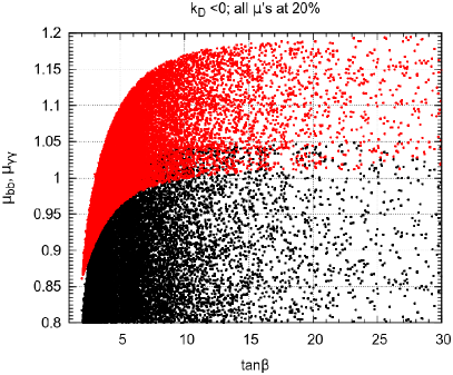
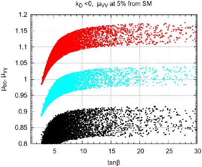
Figure 1: Left panel: Assuming that all $\mu_{f}$ are within 20% of the SM prediction we plot $\mu_{b\bar{b}}$ (red/dark-gray) and $\mu_{\gamma\gamma}$ (black). Right panel: Assuming now that $\mu_{VV}$ are within 5% of the SM prediction we plot the same quantities. For comparison we also plot $\mu_{b\bar{b}}$ (cyan/light-gray) for the assumed production of Ref. FGHS .

This is puzzling, since we can reproduce their remaining plots.

After comparing notes with R. Santos from Ref. FGHS , we found that the difference originates in the gluon fusion production rates, because we are using values from an more recent version of HIGLU Spira:1995mt , and, eventually, different PDF’s and energy scales. For example, they quote

$$\frac{\sigma(gg\rightarrow h)^{\textrm{2HDM}}_{\textrm{NNLO}}}{\sigma(gg\rightarrow h_{\textrm{SM}})_{\textrm{NNLO}}}=1.06\hskip 12.91663pt[\sin{(\beta+\alpha)=1}],$$ (8)

while we, using the latest version (4.0) of HIGLU Spira:1995mt , obtain

$$\frac{\sigma(gg\rightarrow h)^{\textrm{2HDM}}_{\textrm{NNLO}}}{\sigma(gg\rightarrow h_{\textrm{SM}})_{\textrm{NNLO}}}=1.126\hskip 12.91663pt[\sin{(\beta+\alpha)=1}].$$ (9)

This apparently explains why our $\mu_{b\bar{b}}$ result (in red/dark-gray) lies above the one which we obtain (in cyan/light-gray) with the assumed production rates used in Ref. FGHS .

But, this raises another puzzle. If the only difference lies in the production rates, why do our results for $\mu_{\gamma\gamma}$ agree with those in Ref. FGHS ? This is what we turn to in section II.3.

II.2 The crucial importance of $h\rightarrow VV$ and trigonometry

In the previous section, we required that all points obey $0.8\leq\mu_{f}\leq 1.2$ for all final states $VV$, $\tau^{+}\tau^{-}$, $b\bar{b}$, and $\gamma\gamma$, simultaneously. The problem with this procedure is that one misses out on the crucial importance that $\mu_{VV}$ has on its own.

In this section, we only assume that $0.8\leq\mu_{VV}\leq 1.2$, and we will make the cavalier assumption that the production is due exclusively to the gluon fusion with intermediate top, while the decay is due exclusively to the decay $h\rightarrow b\bar{b}$ degenerate . Under these assumptions,

$$\mu_{VV}\approx\frac{k_{U}^{2}}{k_{D}^{2}}\sin^{2}{(\beta-\alpha)}.$$ (10)

We now perform a simple trigonometric exercise. We vary $\alpha$ between $-\pi/2$ and $\pi/2$, $\tan{\beta}$ between $1$ and $30$, and we only keep those regions where $0.8\leq\mu_{VV}\leq 1.2$, with the approximation in Eq. (10).

In Fig. 2, we show the remaining points in the $\sin{\alpha}-\tan{\beta}$ plane.

Figure 2: Left panel: Plot of $\tan\beta$ as a function of $\sin\alpha$ for all the points that obey Eq. (10) with $0.8\leq\mu_{VV}\leq 1.2$. Right panel: Plot of $\sin^{2}(\beta-\alpha)$ as a function of $\tan\beta$ for the points that obey Eq. (10) with $0.8\leq\mu_{VV}\leq 1.2$ and have $k_{D}<0$.

This matches remarkably well the Fig. 2-Left from Ref. FGHS . That is, a simple back of the envelope calculation has most of the Physics. The left branch of the left panel of Fig. 2 corresponds to the SM sign ($k_{D}>0$), and it lies very close to the curve $\sin{(\beta-\alpha)}=1$. The right branch of the same figure corresponds to the wrong sign ($k_{D}<0$), and lies very close to the curve $\sin{(\beta+\alpha)}=1$ rui .

Under the same assumptions, we can draw $\sin^{2}{(\beta-\alpha)}$ as a function of $\tan{\beta}$, as seen in the right panel of Fig. 2, keeping only $\sin{\alpha}>0$ ($k_{D}<0$) points. Notice that $\sin^{2}{(\beta-\alpha)}$ becomes almost univocally defined in terms of $\tan{\beta}$. Indeed, fixing $\tan{\beta}$, and defining the fractional variation of $\sin^{2}{(\beta-\alpha)}$ around its average value by

$$\Delta=\frac{\sin^{2}{(\beta-\alpha)}_{\textrm{max}}-\sin^{2}{(\beta-\alpha)}_{\textrm{min}}}{\sin^{2}{(\beta-\alpha)}_{\textrm{max}}+\sin^{2}{(\beta-\alpha)}_{\textrm{min}}},$$ (11)

we obtain the results in Fig. 3.

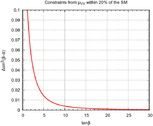
Figure 3: Fractional variation of $\sin^{2}{(\beta-\alpha)}$ as a function of $\tan\beta$ for all points with $k_{D}<0$ that obey Eq. (10) with $0.8\leq\mu_{VV}\leq 1.2$.

For small $\tan{\beta}$, $\sin^{2}{(\beta-\alpha)}$ is determined to better than $10\%$, when $\mu_{VV}$ is fixed only to $20\%$ accuracy. Although it might seem from Eq. (10) that it should be roughly the same, it turns out that the inclusion in Eq. (10) of $k_{U}$ and $k_{D}$ from Eqs. (1)-(2) helps in reducing the error. But things get even more accurate as $\tan{\beta}$ increases. For example, for $\tan{\beta}=10$, $\sin^{2}{(\beta-\alpha)}$ differs very little from unity, and it is even more precisely defined around its average value; an accuracy better than $0.5\%$, coming from a $\mu_{VV}$ fixed only to $20\%$ accuracy.

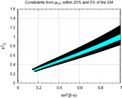
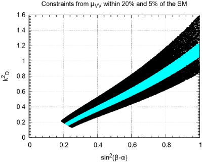
Figure 4: Left panel: $k^{2}_{D}$ as a function of $\sin^{2}{(\beta-\alpha)}$ for all points with $k_{D}<0$ that obey Eq. (10) with $0.8\leq\mu_{VV}\leq 1.2$ (black) or with $0.95\leq\mu_{VV}\leq 1.05$ (cyan/light-gray). Right panel: The same but for generated data obeying the model constraints.

Finally, in the left panel of Fig. 4 we show $k_{D}^{2}$ as a function of $\sin^{2}{(\beta-\alpha)}$, under the same assumptions (black). For comparison, we show how this relation becomes more constrained if we require $0.95\leq\mu_{VV}\leq 1.05$ (cyan/light-gray). To emphasize that the trigonometric relations which result from $\mu_{VV}$ in Eq. (10) explain most of the results, we show in the right panel of Fig. 4 the same plot but now with points generated obeying all the model constraints and without the simplifying assumptions that led to Eq. (10). These simple considerations will turn out to be very important in the next section.

II.3 How production affects the rates

In the previous section, we have made a drastic approximation, which reduced the analysis to a simple trigonometric issue in $\alpha$ and $\beta$, with no dependence on other 2HDM parameters. Now we resume the SET found by scanning all the 2HDM parameter space and imposing theoretical constraints, as defined at the beginning of section II; we then use all production mechanisms.

In Fig. 5, we show our 8 TeV results for $k_{D}^{2}$ as a function of $\sin^{2}{(\beta-\alpha)}$. In black, we see the points generated from the SET, constrained exclusively by $0.8\leq\mu_{VV}\leq 1.2$.

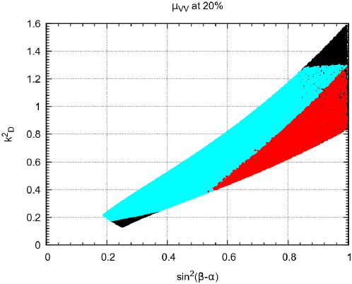
Figure 5: Allowed region for $k^{2}_{D}$ as a function of $\sin^{2}{(\beta-\alpha)}$ for all points with $k_{D}<0$ that obey $0.8\leq\mu_{VV}\leq 1.2$ (black). The region in cyan (light-gray) is obtained by imposing in addition that $0.8\leq\mu_{\tau\tau}\leq 1.2$, while in the region in red (dark-gray) we further impose $0.8\leq\mu_{\gamma\gamma}\leq 1.2$.

This coincides with the black region in the right panel of Fig. 4, and should be compared with the left panel of Fig. 4. As already mentioned, the similarity is uncanny. Simple trigonometry really does have a very strong impact on the results, particularly in the values of $\sin^{2}{(\beta-\alpha)}$; its ranges are practically the same in the two figures. The value for $k_{D}^{2}$ for low $\sin^{2}{(\beta-\alpha)}$ (which, as we see from the right panel of Fig. 2, occurs for low $\tan{\beta}$), is also rather similar. There are, of course, minor quantitative differences: some due to the fact that the SET already has some constraints on the model parameters, due to the imposition of the bounded from below, perturbativity and $S$, $T$, $U$ conditions; some due to the details of the production mechanism. The most important difference occurs for $\sin^{2}{(\beta-\alpha)}\sim 1$ (large $\tan{\beta}$), where $k_{D}^{2}\sim 1\pm 0.2$ in Fig. 4, while $k_{D}^{2}\sim 1.2\pm 0.4$ in Fig. 5. This, as we shall see, is rooted in the production.

It is also interesting to compare Fig. 5, with Fig. 6, which we have drawn using the assumed production rates in Ref. FGHS . Notice that the values of $k_{D}^{2}$ are now smaller, especially for $\sin^{2}{(\beta-\alpha)}\sim 1$ (large $\tan{\beta}$).

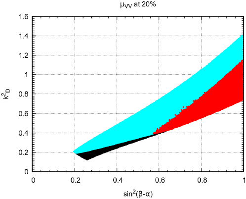
Figure 6: Same as in Fig. 5, but for the assumed production rates in Ref. FGHS . See text for details.

It is easy to see that imposing further $0.8\leq\mu_{\tau^{+}\tau^{-}}\leq 1.2$ may not make a substantial difference. To understand qualitatively the impact of channels other than $h\rightarrow VV$, let us assume that all observed decays will be measured at the SM rates, with the same error $\delta$. Using Eqs. (6)-(7), we find

$$1\pm 2\delta\sim\frac{\mu_{f_{1}}}{\mu_{f_{2}}}=\frac{R_{D}^{f_{1}}}{R_{D}^{f_{2}}}$$ (12)

for all final states $f_{1}$ and $f_{2}$. Notice that this relation does not depend on the production rate, nor on the total width ratios, which are the same for all decays. In particular,

$$\frac{\mu_{\tau^{+}\tau^{-}}}{\mu_{VV}}=\frac{k_{D}^{2}}{\sin^{2}{(\beta-\alpha)}},$$ (13)

where we have used Eqs. (2)-(3). This means that, roughly speaking, $k_{D}^{2}$ should lie between the lines $k_{D}^{2}=0.6\,\sin^{2}{(\beta-\alpha)}$ and $k_{D}^{2}=1.4\,\sin^{2}{(\beta-\alpha)}$, when we consider points which pass current data at around $20\%$. Close to $\sin^{2}{(\beta-\alpha)}\sim 1$, this should reduce the range of $k_{D}^{2}$ from $(0.8,\,1.6)$ to, roughly $(0.8,\,1.4)$. We did the corresponding simulation (shown in the cyan/light-gray region of Fig. 5) and find roughly $(0.8,\,1.3)$. Notice that adding $h\rightarrow b\bar{b}$, assuming that it is produced/measured in all channels with the same $20\%$ error, has no impact, because it would lead to the same Eq. (13). So, we might as well leave it out. Before closing the discussion on the $0.8<\mu_{\tau^{+}\tau^{-}}<1.2$ cut, let us explain why this has a small effect on Fig. 5, with our production, and has almost no effect on Fig. 6. The reason is that smaller values of $k^{2}_{D}$ also imply that the ratio $\mu_{\tau^{+}\tau^{-}}$ is smaller and this explains why most points that passed the $\mu_{VV}$ cut at 20% (black) also pass the cut in $\mu_{\tau^{+}\tau^{-}}$ (cyan/light-gray). The black points in Fig. 6 are behind the cyan(light-gray) points and only appear for small values of $k^{2}_{D}$, due to the lower cut on $\mu_{\tau^{+}\tau^{-}}$.

Fig. 5 also shows in red/dark-gray the points generated from the SET, and constrained by $0.8\leq\mu_{\gamma\gamma}\leq 1.2$, in addition to the constraints $0.8\leq\mu_{VV}\leq 1.2$ and $0.8\leq\mu_{\tau^{+}\tau^{-}}\leq 1.2$. Thus, the combination of $VV$, $\tau^{+}\tau^{-}$, and $\gamma\gamma$ constraints forces $\sin^{2}{(\beta-\alpha)}>0.5$. We recall that, from $h\rightarrow VV$ alone, $\sin^{2}{(\beta-\alpha)}\sim 1$ for $\tan{\beta}>10$, with a minute spread.

We now turn to a qualitative understanding of the impact of the differing production rates in Figs. 5 and 6. If all production occurred through gluon fusion with an intermediate top, then the answer would be that an increase in production rates would have no impact at all, because it would cancel in Eq. (II), and we would still have $R_{P}=k_{U}^{2}$. In the SM, the production is indeed dominated by gluon fusion with an intermediate top. But, for the gluon fusion in the 2HDM, the interference with an intermediate bottom becomes important. Indeed, let us write

$$\sigma^{\textrm{2HDM}}(gg\rightarrow h)=k_{U}^{2}\,g_{tt}+k_{U}\,k_{D}\,g_{tb}+k_{D}^{2}\,g_{bb},$$ (14)

where $g_{bb}\ll|g_{tb}|\ll g_{tt}$. In the SM, $k_{U}=k_{D}=1$, and $\sigma^{\textrm{SM}}(gg\rightarrow h)\sim g_{tt}$. Thus, assuming that all production goes through gluon fusion, we find from Eq. (II)

$$R_{P}\sim k_{U}^{2}\left[1+\frac{k_{D}}{k_{U}}\frac{g_{tb}}{g_{tt}}\right].$$ (15)

where we have neglected $g_{bb}$ (we have verified that this is indeed a very good approximation). This equation has many features that one would expect. If the interference is very small, $k_{D}g_{tb}/(k_{U}g_{tt})\ll 1$, and we recover $R_{P}\sim k_{U}^{2}$, as mentioned above. If one were to increase $g_{tb}$ and $g_{tt}$ by the same multiplicative factor, then $R_{P}$ would not be altered. So, what is crucial in the difference between Figs. 5 and 6 is that the mix of $g_{tb}$ and $g_{tt}$ has been altered between the simulations, with $|g_{tb}|/g_{tt}$ becoming larger with the production rates used in this article. This is more important for large values of

$$\frac{k_{D}}{k_{U}}=-\tan{\alpha}\tan{\beta}\sim-\,\sqrt{\frac{\sin^{2}{(\beta-\alpha)}}{\mu_{VV}}}.$$ (16)

The approximation at the end would hold if we were to keep the assumptions of section II.2. The first equality in Eq. (16) would lead us to believe that the second term in Eq. (15) is much more important as $\tan{\beta}$ increases. However, this is mitigated by the fact that, as the analysis in section II.2 and the approximation at the end of Eq. (16) show, $k_{D}/k_{U}$ is tied to $\sin^{2}{(\beta-\alpha)}/\mu_{VV}$. Indeed, the right panel of Fig. 1, obtained with a full simulation, shows that there are effects of differing production rates as low as $\tan{\beta}\sim 1$. Before proceeding, it is useful to stress this point. The intuition gained by looking at the dependence of the couplings on $\alpha$ and $\beta$, such as in the first equality in Eq. (16), can be completely altered once some experimental bound is imposed, such as the $\mu_{VV}$ seen in the approximation at the end of Eq. (16), because the bound may impose rather nontrivial constraints between $\alpha$ and $\beta$. In this case, for each $\tan{\beta}$, the range of allowed $\alpha$ is correlated and very small.

Having established that $R_{P}$ is larger in our simulation than in the simulation of Fig. 6, we must now understand its differing impact on $\mu_{\gamma\gamma}$, which is almost the same, and on $\mu_{b\bar{b}}$, which increases.

The crucial point comes from the previous section, where we found that $0.8\leq\mu_{VV}\leq 1.2$ alone gives a very tight constraint on the possible values of $k_{V}^{2}=\sin^{2}{(\beta-\alpha)}$, for a given value of $\tan{\beta}$. Thus, for fixed $\tan{\beta}$, if we wish to keep $\mu_{VV}=R_{P}k_{V}^{2}R_{TW}$ constant and close to one, we must always keep $R_{P}R_{TW}\simeq\textrm{constant}$. As a result, the only way to accommodate an increased production is to have a decreased $R_{TW}$ (which is roughly determined by $1/k_{D}^{2}$), and to increase $k_{D}^{2}$. This explains why $k_{D}^{2}$ is larger when we use the larger $|g_{tb}|/g_{tt}$, as in Fig. 5, than it is when we use the smaller production $|g_{tb}|/g_{tt}$, as in Fig. 6. Since $k_{D}^{2}$ appears in both $h\rightarrow b\bar{b}$ and $h\rightarrow\tau^{+}\tau^{-}$, both are increased in our simulation.

If we were to take the right panel of Fig. 1 at face value, we might have been led to conclude that a measurement $0.9\leq\mu_{b\bar{b}}\leq 1.1$ or $0.9\leq\mu_{\tau^{+}\tau^{-}}\leq 1.1$ would already exclude the $k_{D}<0$ solution for large $\tan{\beta}$, as can be seen in the right panel of Fig. 1 (red/dark-gray region). Unfortunately, as we have shown, these rates are extremely sensitive to the production and, thus, cannot be used to exclude $k_{D}<0$.

In contrast, because, for fixed $\tan{\beta}$, $\mu_{VV}$ implies roughly that $R_{P}R_{TW}\simeq\textrm{constant}$, $\mu_{\gamma\gamma}$ is virtually independent of the production and only depends on the decay rate $h\to\gamma\gamma$. As the largest contribution to this decay comes from the $W$ boson diagrams, and this coupling is already fixed by $\mu_{VV}$, $\mu_{\gamma\gamma}$ will be rather insensitive to the QCD corrections in the production and can be used to constrain $k_{D}<0$. As a result, our prediction for $\mu_{\gamma\gamma}$ in the right panel of Fig. 1 mirrors that in Fig. 5-Left of Ref. FGHS .

The black points in the right panel of Fig. 1 represent the allowed region for $\mu_{\gamma\gamma}$ when we take $0.95\leq\mu_{VV}\leq 1.05$. As the highest value for this range is only slightly above 0.9, we agree with the conclusion of Ref. FGHS that a putative $5\%$ measurement of $h\rightarrow\gamma\gamma$ at 8 TeV around the SM value would rule out $k_{D}<0$.

In summary, the constraint $R_{P}R_{TW}\simeq\textrm{constant}$ means that, when we increase the $|g_{tb}|/g_{tt}$ mix in the production rates, $\mu_{\gamma\gamma}$ will stay the same, as we have found in Fig. 1. In contrast, since an increased production implies an increased $k_{D}^{2}$, we find that $\mu_{b\bar{b}}=\mu_{\tau^{+}\tau^{-}}=R_{P}k_{D}^{2}R_{TW}\simeq\textrm{constant}\ k_{D}^{2}$ must increase, in accordance with what we see in the same figure.

There are three points to note. First, the next LHC run will occur at 14 TeV, while the current data exists for 8 TeV. Second, the same argument that showed that $\mu_{\gamma\gamma}$ is stable against changes in production can be applied to $\mu_{Z\gamma}$. Third, the same delayed decoupling effect found in $\mu_{\gamma\gamma}$ appears in $\mu_{Z\gamma}$. We address these issues in the next section.

III Predictions for the 14 TeV run

Strictly speaking, future LHC experiments will be carried out at 14 TeV. Moreover, the dominant gluon fusion process shifts by almost a factor of $2.5$ in going from $8$ to $14$ TeV. Naively, when $\tan{\beta}$ becomes large, the interference between the dominant gluon fusion through a top triangle and the gluon fusion through a bottom triangle becomes important, and then the sign of $k_{D}$ is crucial. However, as we have already pointed out, things are complicated by the fact that $k_{D}/k_{U}$ is tied to $\sin^{2}{(\beta-\alpha)}/\mu_{VV}$, and current experiments keep $\sin^{2}{(\beta-\alpha)}>0.5$. Moreover, in gluon fusion, the magnitude squared of the top triangle, the magnitude squared of the bottom triangle, and the interference are multiplied by almost the same factor as one goes from 8 to 14 TeV. As a result, most points that only differ from the SM model measurements by, say, $20\%$ at 8 TeV will also differ from the SM model measurements by $20\%$ at 14 TeV, when we use our production based on the current version of HIGLU with specific PDF’s and energy scales. We have performed a simulation with 146110 points to test this issue. Only 800 of those (around $0.6\%$), pass the $20\%$ test at 8 TeV but not at 14 TeV. So, the conclusions are unaffected by this issue.

In any case, we perform here the following analysis. We first find points (satisfying the conditions in the SET) which differ from the SM at 8 TeV by $20\%$. Then, we use those 2HDM points to generate all rates at 14 TeV. Our subsequent discussions of the $\mu$ parameters and, in particular, on the impact of $h\rightarrow Z\gamma$, are only based on the surviving points.

Assuming current experiments ($20\%$ errors at 8 TeV), our predictions for $\mu_{\tau^{+}\tau^{-}}$ (in red/dark-gray) and $\mu_{\gamma\gamma}$ (in black) are shown on the left panel of Fig. 7.

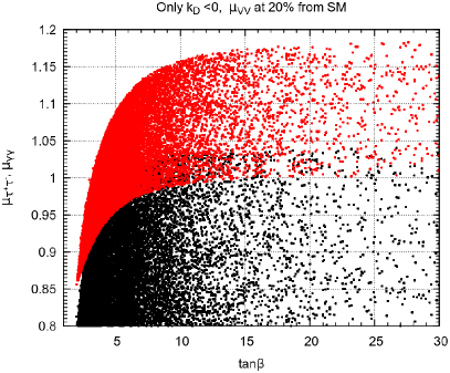
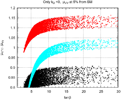
Figure 7: Left panel: Prediction for $\mu_{\tau^{+}\tau^{-}}$ (red/dark-gray) and $\mu_{\gamma\gamma}$ (black) as a function of $\tan\beta$ for the LHC at 14 TeV with the constraint of $20\%$ errors at 8 TeV. Right panel: Assuming now that $\mu_{VV}$ are within 5% of the SM prediction at 14TeV, we plot the same quantities. Also shown (cyan/light-gray) is the prediction for $\mu_{b\bar{b}}(Vh)$ from associated production.

We see that, at this level of precision, we cannot rule out the $k_{D}<0$ branch.

If we now imagine that, in addition, the $\mu_{VV}$ are measured at 14 TeV to lie around unity with a $5\%$ precision, then we obtain for $\mu_{\tau^{+}\tau^{-}}$ (in red/dark-gray) and $\mu_{\gamma\gamma}$ (in black) in the right panel of Fig. 7. Here, we would be led to conclude that a $5\%$ measurement of $\mu_{\tau^{+}\tau^{-}}\sim 1$ would exclude $k_{D}<0$ for large $\tan{\beta}$. As explained in the previous section, this conclusion is misleading since the $\mu_{\tau^{+}\tau^{-}}$ (and the $\mu_{b\bar{b}}$ rates, combining all production modes) depend crucially on the detailed mix of the gluon production through intermediate tops and bottoms. Thus, we agree with Ref. FGHS that a $5\%$ measurement of $\mu_{\gamma\gamma}$ can be used to exclude the wrong-sign solution, while $\mu_{\tau^{+}\tau^{-}}$ should not.

We recall that the $\mu_{b\bar{b}}$ we present (in red/dark-gray) in Fig. 1 was calculated assuming that $b\bar{b}$ is measured in all channels, and using our production rates. In that case, it would seem that a $5\%$ of $\mu_{b\bar{b}}$ could exclude $k_{D}<0$. However, as with $\mu_{\tau^{+}\tau^{-}}$, the result is very sensitive to the production, and, thus, cannot be used to probe $k_{D}<0$. In foreseeing the 14 TeV run, we differ from Ref. FGHS , and study $b\bar{b}$ only in the $Vh$ production channel, shown in cyan/light-gray on the right panel of Fig. 7. Unfortunately, in contrast with what happens with our $\mu_{b\bar{b}}$ in Fig. 1, a $5\%$ measurement of $\mu_{b\bar{b}}(Vh)$ is centered around unity for $\tan{\beta}>10$, and, thus, it cannot be used to preclude $k_{D}<0$.

We now turn our attention to the decay $h\rightarrow Z\gamma$. As mentioned above, there are three good reasons to look at this decay. First, the decay will be probed at LHC’s Run2, and there are already upper bounds on it from Run1. Second, as for $\mu_{\gamma\gamma}$, we did not find a significant difference when using different production rates. Third, the delayed decoupling that has been used in showing the usefulness of a future measurement of $\mu_{\gamma\gamma}$ is also present in $\mu_{Z\gamma}$. The expressions for this decay can be found in Ref. HHG , which we have checked.

Starting from the SET, we calculated $\mu$ for $VV$, $\gamma\gamma$, and $\tau^{+}\tau^{-}$ at 8 TeV, requiring that all lie within $20\%$ of the SM. The remaining points were required to pass $\mu_{VV}$, within $5\%$ of the SM, at 14 TeV. We then calculated $\mu_{Z\gamma}$, $\mu_{\tau^{+}\tau^{-}}$ and $\mu_{\gamma\gamma}$. Our results are shown in Fig. 8.

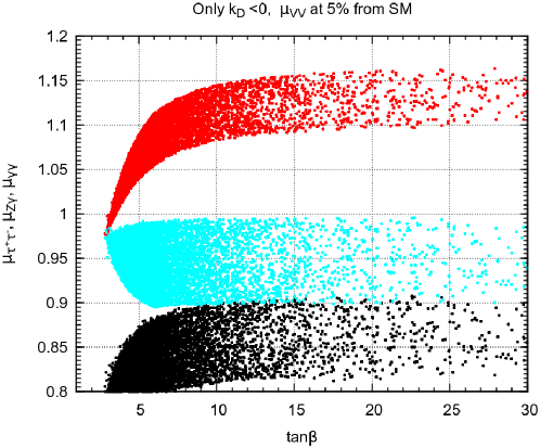
Figure 8: Prediction for $\mu_{\tau^{+}\tau^{-}}$ (red/dark-gray), $\mu_{Z\gamma}$ (cyan/light-gray) and $\mu_{\gamma\gamma}$ (black) as a function of $\tan\beta$, for the LHC at 14 TeV, with a measurement of $\mu_{VV}$ within $5\%$ of the SM at 14 TeV.

There are bad news and good news.

The bad news comes from the fact that the results in Fig. 8 show that $\mu_{Z\gamma}\lesssim 1$. Therefore, this channel cannot be used to exclude the $k_{D}<0$ solution. The good news are the following. The ratio $\mu_{VV}$, even at 20%, puts a strong bound on $\mu_{Z\gamma}$. In fact, we found that, for $k_{D}<0$ and before applying the $\mu_{VV}$ constraint, $\mu_{Z\gamma}$ could be as large as two for $\mu_{\gamma\gamma}\sim 1$, as shown in the black region of Fig. 9.

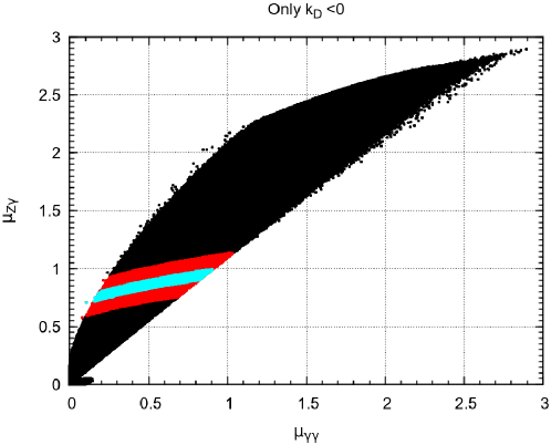
Figure 9: Predictions for $\mu_{Z\gamma}$ versus $\mu_{\gamma\gamma}$ at 14 TeV, for $k_{D}<0$. In black, we have the points in the SET (obeying theoretical constraints and $S,T,U$, only). In red/dark-gray (cyan/light-gray), the points satisfying in addition $VV$ within $20\%$ ($5\%$) of the SM, at 14 TeV.

However, the requirement that $\mu_{VV}$ should be within 20% of the SM drastically limits this upper bound, requiring it to be very close to the SM value, as shown in the red/dark-gray region of Fig. 9. If we require a measurement of $\mu_{VV}$ to be within 5% of the SM (cyan/light-gray region of Fig. 9), then both $\mu_{\gamma\gamma}$ and $\mu_{Z\gamma}$ have to be below their SM values for $k_{D}<0$. We find that this effect is more predominant in $\gamma\gamma$ ($\mu_{\gamma\gamma}<0.9$) than in $Z\gamma$ ($\mu_{Z\gamma}<1$).

Having discussed what we can learn from $\mu_{\gamma\gamma}$ and $\mu_{Z\gamma}$ for the wrong-sign branch, $k_{D}<0$, we can ask what is the situation with the normal branch, $k_{D}>0$.

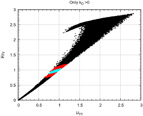
Figure 10: Predictions for $\mu_{Z\gamma}$ versus $\mu_{\gamma\gamma}$ at 14 TeV, for $k_{D}>0$. In black, we have the points in the SET (obeying theoretical constraints and $S,T,U$, only). In red/dark-gray (cyan/light-gray), the points satisfying in addition $VV$ within $20\%$ ($5\%$) of the SM, at 14 TeV.

This is shown in Fig. 10. We see that even before requiring any constraint on $\mu_{VV}$ (black points), there is only a very small region with large $\mu_{Z\gamma}$ which is compatible with $0.8\leq\mu_{\gamma\gamma}\leq 1.2$ from current LHC data. In particular, points from the SET, with $\mu_{\gamma\gamma}\sim 1$ and $\mu_{Z\gamma}\sim 2$, allowed for $k_{D}<0$ in the black region of Fig. 9, are almost forbidden for $k_{D}>0$ in the black region of Fig. 10. If we further require $\mu_{VV}$ to be within 20% (red/dark-gray) or 5% (cyan/light-gray) both $\mu_{\gamma\gamma}$ and $\mu_{Z\gamma}$ have to be close to the SM values, with a wider range allowed for $\mu_{\gamma\gamma}$.

We conclude that, for both signs of $k_{D}$, current bounds on $\mu_{VV}$ already preclude a value of $\mu_{Z\gamma}>1.5$ from being compatible with the usual 2HDM with softly broken $Z_{2}$. A measurement in the next LHC run of $\mu_{VV}$ lying within $5\%$ of the SM will essentially force $\mu_{Z\gamma}\lesssim 1$ for $k_{D}<0$ and $\mu_{Z\gamma}\lesssim 1.05$ for $k_{D}>0$.

IV Predictions for the Flipped 2HDM

In this section, we analyze the Flipped 2HDM. This coincides with the Type II 2HDM, except that the charged leptons couple to the Higgs proportionally to $k_{U}$ (not $k_{D}$).

We recall that $\mu_{\tau^{+}\tau^{-}}$ does not have a big effect in Fig. 5, for the Type II 2HDM. This has a simple explanation, through the approximation in Eq. (13). In the Flipped 2HDM, the same approximation yields

$$\frac{\mu_{\tau^{+}\tau^{-}}}{\mu_{VV}}=\frac{k_{U}^{2}}{\sin^{2}{(\beta-\alpha)}},$$ (17)

leading one to suspect that $\mu_{\tau^{+}\tau^{-}}$ might have a larger effect here. This is confirmed in the left panel of Fig. 11, where we show our 8 TeV results for $k_{D}^{2}$ as a function of $\sin^{2}{(\beta-\alpha)}$.

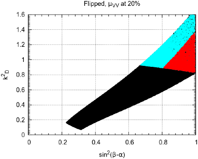
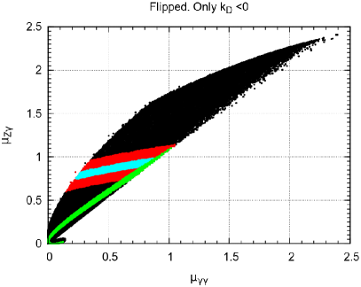
Figure 11: Left panel: Allowed region for $k^{2}_{D}$ as a function of $\sin^{2}{(\beta-\alpha)}$ in the Flipped 2HDM, for all points with $k_{D}<0$ that obey $0.8\leq\mu_{VV}\leq 1.2$ (black). The region in cyan (light-gray) is obtained by imposing in addition that $0.8\leq\mu_{\tau\tau}\leq 1.2$, while in the region in red (dark-gray) we further impose $0.8\leq\mu_{\gamma\gamma}\leq 1.2$. Right panel: Predictions for $\mu_{Z\gamma}$ versus $\mu_{\gamma\gamma}$ at 14 TeV, for $k_{D}<0$, in the Flipped 2HDM. In black, we have the points in the SET (obeying theoretical constraints and $S,T,U$, only). In red/dark-gray (cyan/light-gray), the points satisfying in addition $VV$ within $20\%$ ($5\%$) of the SM, at 14 TeV. Shown in green/light-gray are the points satisfying $\mu_{\tau^{+}\tau^{-}}$ at $20\%$ of the SM, which lie on a line going diagonally from the origin with almost unit slope.

The colour codes, explained in the figure caption, mirror those in Fig. 5. Here the $20\%$ measurement of $\mu_{\tau^{+}\tau^{-}}$ does have a big impact.

However, one might suspect that this may not change much the conclusions on $\gamma\gamma$ and $Z\gamma$, because, as mentioned before, those were primarily determined by the constraint on $\mu_{VV}$. This is what we find in the right panel of Fig. 11. The effect of $\mu_{\tau^{+}\tau^{-}}$ is to reduce the allowed region by a very fine slice, shown in the right panel of Fig. 11 as a green/light-gray line going diagonally from the origin with almost unit slope. This figure should be compared with Fig. 9, which holds in the Type II 2HDM. In both cases, a $5\%$ measurement of $\mu_{\gamma\gamma}$ ($\mu_{Z\gamma}$) will (will not) exclude $k_{D}<0$.

V Conclusions

We have analysed the Type II 2HDM with softly broken $Z_{2}$, scrutinizing the possibility that the $hb\bar{b}$ coupling has a sign opposite to that in the SM and the impact on this issue of $Z\gamma$. We impose the usual theoretical constraints, assuming that $\mu_{VV}$, $\mu_{\tau^{+}\tau^{-}}$, and $\mu_{\gamma\gamma}$ differ from the SM by no more than $20\%$ at 8 TeV. We found that the constraint from $\mu_{VV}$ is crucial, and can be understood in simple trigonometric terms. In particular, we show that this cut has a rather counter-intuitive implication. Before this cut is applied, it would seem that the importance of the bottom-mediated gluon fusion production mechanism would grow linearly with $\tan{\beta}$. However, after current bounds are placed on $\mu_{VV}$, the importance of the bottom-mediated gluon fusion production mechanism grows asymptotically into a constant, for large $\tan{\beta}$. This generalizes as a cautionary tale: applying a new experimental bound may force unexpected relations among the parameters, and the theoretical intuition must be revised in this new framework.

In projecting to the future, we have then simulated our points at 14 TeV, highlighting the fact, for the issues that interest us, using the current version of HIGLU at 14 TeV or at 8 TeV leads to the same results. We have shown that results for the $b\bar{b}$ and $\tau^{+}\tau^{-}$ depend sensitively on the ratio $g_{tb}/g_{tt}$ encoding the relative weight of the square of the top-mediated gluon fusion production amplitude, and the interference of this amplitude with the bottom-mediated gluon fusion production amplitude. As a result, these channels should not be used to probe the $k_{D}<0$ possibility. Even if that were not the case, since $b\bar{b}$ is only measured in associated production and, as we show, $\mu_{b\bar{b}}(Vh)$ includes unity, this channel would not be useful.

In contrast, in our simulations both $\gamma\gamma$ and $Z\gamma$ are roughly independent of $g_{tb}/g_{tt}$. In addition, they exhibit delayed decoupling in the $hH^{+}H^{-}$ vertex. As a result, they could, in principle, be used to probe the $k_{D}<0$ possibility. Indeed, as found in Ref. FGHS , a 5% measurement of $\mu_{\gamma\gamma}$ around unity will be able to exclude $k_{D}<0$.

We then performed a detailed analysis of $Z\gamma$. We show that, before including the LHC data, values of $\mu_{\gamma\gamma}$ and $\mu_{Z\gamma}$ were allowed between $0$ and $3$, but with a correlation between the two, as shown in the black regions of Fig. 9 and Fig. 10. This correlation is more important (that is, the region in the figure is smaller) for $k_{D}>0$ than it is for $k_{D}<0$. In particular, $\mu_{\gamma\gamma}\sim 1$ with $\mu_{Z\gamma}\sim 2$ would be possible in the latter case, but not in the former. Things change dramatically when the simple constraint $0.8<\mu_{VV}<1.2$ is imposed. In that case, we obtain the red/dark-gray regions of Fig. 9 ($k_{D}<0$) and Fig. 10 ($k_{D}>0$). This already places $\mu_{\gamma\gamma}$ and $\mu_{Z\gamma}$ close to the SM, although, strictly speaking, points with $\mu_{\gamma\gamma}=1$ with $\mu_{Z\gamma}=1$ are not allowed in our simulation when $k_{D}<0$. A $5\%$ measurement of $VV$ around the SM at 14 TeV will bring $\mu_{Z\gamma}$ closer to unity, for $k_{D}>0$, and just below unity, for $k_{D}<0$. Thus, this decay cannot be used to exclude $k_{D}<0$.

But we have the reverse advantage. It is obvious that a measurement of $\mu_{Z\gamma}>1$ would exclude the SM. We have shown that a 5% precision on $\mu_{VV}$ around the SM, together with $\mu_{Z\gamma}>1$, would also exclude $k_{D}<0$, and, together with $\mu_{Z\gamma}>1.1$, would exclude altogether the Type II 2HDM with softly broken $Z_{2}$. If $\mu_{Z\gamma}$ turns out to lie a mere $20\%$ above the SM value, then the softly broken Type II 2HDM is not the solution.

Finally, we analyzed the Flipped 2HDM. Although there is a substantial difference in the $k_{D}^{2}$ versus $\sin^{2}{(\beta-\alpha)}$ plane, this does not change dramatically the $\mu_{\gamma\gamma}$–$\mu_{Z\gamma}$ correlation. As a result, here $5\%$ measurements of $VV$ and $\gamma\gamma$ around the SM at 14 TeV will be enough to exclude $k_{D}<0$, while $\mu_{Z\gamma}$ will not.

- (1) G. Aad et al. [ATLAS Collaboration], Phys. Lett. B 716, 1 (2012) [arXiv:1207.7214 [hep-ex]].
- (2) S. Chatrchyan et al. [CMS Collaboration], Phys. Lett. B 716, 30 (2012) [arXiv:1207.7235 [hep-ex]].
- (3) Up to date results can be found in ATLAS Collaboration, https://twiki.cern.ch/twiki/bin/view/AtlasPublic/HiggsPublicResults; and in CMS Collaboration, https://twiki.cern.ch/twiki/bin/view/CMSPublic/PhysicsResultsHIG.
- (4) D. Carmi, A. Falkowski, E. Kuflik and T. Volansky, JHEP 1207, 136 (2012) [arXiv:1202.3144 [hep-ph]].
- (5) C. -W. Chiang and K. Yagyu, JHEP 1307, 160 (2013) [arXiv:1303.0168 [hep-ph]].
- (6) A. Barroso, P. M. Ferreira, R. Santos, M. Sher and J. P. Silva, arXiv:1304.5225 [hep-ph], talk given by R. Santos at Toyama International Workshop on Higgs as a Probe of New Physics (13-16, February, 2013).
- (7) P. M. Ferreira, J. F. Gunion, H. E. Haber and R. Santos, arXiv:1403.4736 [hep-ph].
- (8) J. F. Gunion, H. E. Haber, G. L. Kane and S. Dawson, “The Higgs Hunter’s Guide,” Front. Phys. 80, 1 (2000).
- (9) G. C. Branco, P. M. Ferreira, L. Lavoura, M. N. Rebelo, M. Sher and J. P. Silva, Phys. Rept. 516, 1 (2012) [arXiv:1106.0034 [hep-ph]].
- (10) P. Posch, Phys. Lett. B 696, 447 (2011) [arXiv:1001.1759 [hep-ph]].
- (11) N. D. Christensen and C. Duhr, Comput. Phys. Commun. 180, 1614 (2009), [arxiv:0806.4194].
- (12) A. Arhrib, M. Capdequi Peyranere, W. Hollik and S. Penaranda, Phys. Lett. B 579, 361 (2004) [hep-ph/0307391].
- (13) G. Bhattacharyya, D. Das, P. B. Pal and M. N. Rebelo, JHEP 1310, 081 (2013) [arXiv:1308.4297 [hep-ph]].
- (14) S. Chatrchyan et al. [CMS Collaboration], Phys. Rev. D 89, 012003 (2014) [arXiv:1310.3687 [hep-ex]].
- (15) B. Tuchming, (for the CDF and D0 Collaborations) arXiv:1405.5058 [hep-ex].
- (16) G. Aad et al. [ATLAS Collaboration], Phys. Lett. B 732, 8 (2014) [arXiv:1402.3051 [hep-ex]].
- (17) S. Chatrchyan et al. [CMS Collaboration], Phys. Lett. B 726, 587 (2013) [arXiv:1307.5515 [hep-ex]].
- (18) N. G. Deshpande and E. Ma, Phys. Rev. D 18, 2574 (1978).
- (19) S. Kanemura, T. Kubota and E. Takasugi, Phys. Lett. B 313, 155 (1993) [hep-ph/9303263].
- (20) A. G. Akeroyd, A. Arhrib and E. -M. Naimi, Phys. Lett. B 490, 119 (2000) [hep-ph/0006035].
- (21) I. F. Ginzburg and I. P. Ivanov, hep-ph/0312374.
- (22) W. Grimus, L. Lavoura, O. M. Ogreid and P. Osland, Nucl. Phys. B 801, 81 (2008) [arXiv:0802.4353 [hep-ph]].
- (23) M. Baak, M. Goebel, J. Haller, A. Hoecker, D. Kennedy, R. Kogler, K. Moenig and M. Schott et al., Eur. Phys. J. C 72, 2205 (2012) [arXiv:1209.2716 [hep-ph]].
- (24) M. Spira, hep-ph/9510347.
- (25) R. V. Harlander, S. Liebler and H. Mantler, Computer Physics Communications 184, 1605 (2013) [arXiv:1212.3249 [hep-ph]].
- (26) https://twiki.cern.ch/twiki/bin/view/LHCPhysics/CrossSectionsFigures .
- (27) P. M. Ferreira, R. Santos, H. E. Haber and J. P. Silva, Phys. Rev. D 87, 055009 (2013) [arXiv:1211.3131 [hep-ph]].