Interferometry of chemically peculiar stars:
theoretical predictions vs. modern observing facilities

Abstract

By means of numerical experiments we explore the application of interferometry to the detection and characterization of abundance spots in chemically peculiar (CP) stars using the brightest star $\varepsilon$ UMa as a case study. We find that the best spectral regions to search for spots and stellar rotation signatures are in the visual domain. The spots can clearly be detected already at a first visibility lobe and their signatures can be uniquely disentangled from that of rotation. The spots and rotation signatures can also be detected in NIR at low spectral resolution but baselines longer than $180$ m are needed for all potential CP candidates. According to our simulations, an instrument like VEGA (or its successor e.g., FRIEND) should be able to detect, in the visual, the effect of spots and spots+rotation, provided that the instrument is able to measure $V^{2}\approx 10^{-3}$, and/or closure phase. In infrared, an instrument like AMBER but with longer baselines than the ones available so far would be able to measure rotation and spots. Our study provides necessary details about strategies of spot detections and the requirements for modern and planned interferometric facilities essential for CP star research.

1 Introduction

Optical and infrared interferometry is a powerful observational technique capable of reaching a very high angular resolution. Potentially, interferometry allows one to derive not only the sizes of stellar objects, but, under the conditions of sufficient spatial coverage, even to reconstruct the details on the stellar surfaces. First successful applications of interferometry to imaging the stellar surfaces were carried out for supergiants (Che et al. 2011; Zhao et al. 2009; Monnier et al. 2007) and giants (Chiavassa et al. 2010; Le Bouquin et al. 2009) that have large angular diameters because of their large sizes.

The application of interferometry to main-sequence (MS) stars, unfortunately, is still limited to only brightest objects. Modern facilities are capable of resolving the closest and/or largest MS stars and measure their diameters already on a regular basis (e.g. Boyajian et al. 2013; Maestro et al. 2013). But the detailed study of surface morphology is still a challenging task for most of them.

Among MS stars there is one class of objects that obviously deserves interferometric attention – chemically peculiar (CP) stars. These stars possess strong abundance inhomogeneities in their atmospheres where atoms and ions of certain elements tend to accumulate at different regions on the stellar surface driven by diffusion processes (Michaud 1970). The abundance inhomogeneities on CP stars are usually obtained by a mapping technique known as Doppler Imaging (DI) (e.g. Deutsch 1958; Goncharskii et al. 1977) which restores the information about surface abundance inhomogeneities (spots) from the rotational modulated profiles of spectral lines (e.g. Piskunov & Rice 1993; Lüftinger et al. 2010; Kochukhov et al. 2004, for details and some practical applications of the method). Note that the details of inversion problem used to recover spot and rotation information is out of scope of this paper.

Recently, interferometry has been successfully applied to CP stars resulting in a first estimate of the radii of a few stars: $\alpha$ Cir (HD 128898, Bruntt et al. 2008), $\beta$ CrB (HD 137909, Bruntt et al. 2010), $\gamma$ Equ (HD 201601, Perraut et al. 2011), and $10$ Aql (HD 176232, Perraut et al. 2013). Detailed studies of surface morphology of CP stars, however, remain challenging and have never been done so far.

It should be stressed that, in spite of the recent success of DI technique in recovering surface structures of stars, its application is limited to stars rotating fast enough so that rotation dominates the broadening of spectroscopic lines. In other words, the faster the rotation is, the more spectroscopic features can be resolved for a given resolving power of the spectrograph and thus more details on the stellar surface can be studied. However, there are CP stars that rotate very slowly or have small projected rotational velocities, but still show significant spectral variability indicating existence of spots in their atmospheres (e.g., Kochukhov & Ryabchikova 2001; Freyhammer et al. 2008). For those stars no DI is possible, and interferometry thus appears to be a promising technique to study their surface morphology. Interferometry also allows one to derive both the inclination and position angle of stellar rotational axis if sufficient spectral resolution and baseline configurations are provided.

Besides the very few observations available, some authors explored the applications of interferometry to CP stars by means of numerical experiments. In the most recent study by Rousselet-Perraut et al. (2004) authors used two cases of well-known CP stars $\alpha^{2}$ CVn and $\beta$ CrB to explore the possibility to derive the abundance and magnetic maps with interferometric instruments based on fringe phase signals. They concluded that signals from abundance inhomogeneities and magnetic field could be in principle detected in visual and infrared already with modern instruments.

In this work we follow similar ideas outlined in Rousselet-Perraut et al. (2004), but concentrating on the detection of abundance spots in the one of the brightest CP star $\varepsilon$ UMa. This star has a radii of about $4.2R_{\odot}$ (Lueftinger et al. 2003) and distance of $25.31$ pc, which results in one of the largest angular diameter $\theta=1.54$ mas among closest CP stars, and which is easily resolved with modern interferometric instruments. However, contrary to the previous work, we aim to explore the behaviour of wavelength dispersed visibility and closure phase signals, while Rousselet-Perraut et al. (2004) simulated the differential fringe phase.

Our research is based on accurate model atmospheres that predict intensities from abundance maps published in Lueftinger et al. (2003). The same model atmospheres were successfully used in Shulyak et al. (2010) to predict the observed light variability of $\varepsilon$ UMa in narrow and broad-band photometric filters.

2 Overview of modern and planned interferometric facilities

It is essential to compare theoretical predictions that we make in this investigation against available and planned interferometric facilities around the world. Important characteristics of these instruments are the angular resolution, wavelength domain where instrument operate, spectral resolution provided, as well as the sensitivity of detectors in terms of limiting stellar magnitude. Table 1 lists the major facilities and instruments already available and ones that will become available in nearest future to the scientific community. This table does not include instruments that operate in mid-infrared range because CP stars are very faint in there. Most of the information have been adopted from links listed in the OLBIN (Optical Long Baseline Interferometry News) website and references provided therein. In the table, we list four major interferometers that provide long (on the order of tens of meters and longer) baselines: VLTI (Very Large Telescope Interferometer, Cerro Paranal, Chile), CHARA (Center for High Angular Resolution, Mount Wilson, California, USA), SUSI (Sydney University Stellar Interferometer, Australia), and NPOI (Navy Precision Optical Interferometer, Lowell Observatory, Arizona, USA).

Table 1: Interferometric facilities around the world.

Facility	Instrument	Apertures	Sensitivity, $V^{2}_{\rm min}$	Baselines range, m	Wavelength	Resolution, $\lambda/\Delta\lambda$	Limiting magnitude	ref.
VLTI	PIONIER	4	$10^{-5}$ (11)	$11$ – $140$	$H$-band	40	7.5 (ATs)	1
	AMBER	3	$10^{-4}$ (12)		$HK$-bands	$30$, $1500$, $12\,000$	9.0 (UTs)	2
	GRAVITY	4	$10^{-5}$		$K$-band	22, 500, 4 000	10 (UTs)	3
CHARA	JouFLU	2	$10^{-2}$ (13)	$34$ – $331$	$K$-band	$6$	6	4
	VEGA	4	$10^{-2}$ (14)		$480$ – $850$ nm	6 000, 30 000	7.5, 4.5	5,6
	FRIEND	4	$10^{-3}$		$480$ – $850$ nm	6 000, 30 000	7.5, 4.5	14
	MIRC	6	$10^{-4}$ (15)		$H$-band	40	4.5	7
	CLASSIC	2	$>10^{-3}$		$HK$-bands	Broad band	8.5	8
	CLIMB	3	$10^{-3}$ (16)		$K$-band	Broad band	6.5	8
	PAVO	3	$10^{-3}$ (17)		$650$ – $800$ nm	30	8.0	9
SUSI	PAVO	2	$10^{-3}$ (17)	$5$ – $160$, up to $\mathbf{640}$	$550$ – $800$ mn	Broad band	7.0	9
NPOI	VISION	6	$\sim$	$17$ – $437$	$570$ – $850$ mn	$200$ – $1000$	5	10

col. 1 – name of the facility; col. 2 –acronym of the instrument; col. 3 – number of apertures; col. 4 – baseline range; col. 5 – spectral region; col. 6 – spectral resolution; col. 7 – limiting magnitude at the lowest spectral resolution col. 8 – reference to the article describing the instrument

Future new or expected upgrades of the available present interferometric facilities are marked by bold font.

References: (1) Le Bouquin et al. (2011); (2) Petrov et al. (2007); (3) Eisenhauer et al. (2008); (4) Scott et al. (2013); (5) Mourard et al. (2009); (6) Mourard et al. (2011); (7) Monnier et al. (2004); (8) Ten Brummelaar et al. (2013); (9) Ireland et al. (2008); (10) Ghasempour et al. (2012); (11) Montarges et al. (2014); (12) Ohnaka et al. (2009); (13) Mazumdar et al. (2009); (14) Bério et al. (2014); (15) Monnier et al. (2012); (16) O’Brien et al. (2011); (17) Maestro et al. (2013)

3 Methods and simulation setup

The simulations provided in this paper are based on custom numerical routines we have coded in IDL language that compute the complex visibility from a 2D intensity image of the source for the desired set of (u,v) points (Li Causi 2008).

The images of the star were constructed employing abundance maps of elements Ca, Cr, Fe, Mg, Mn, Ti, and Sr obtained with the help of DI technique in Lueftinger et al. (2003). The LLmodels stellar model atmosphere code (Shulyak et al. 2004) was used to compute local model atmospheres. The code computes 1D, LTE model atmospheres and can account for individual abundances of chemical elements. The Stark-broadenined profiles of hydrogen lines were computed using tables of Lemke (1997) based on the VCS theory by Vidal et al. (1973).

Local model atmospheres were calculated for each of $2244$ surface elements of original DI maps ($68$ longitudes and $33$ latitudes). Thus each model atmosphere takes into account local abundance pattern of all mapped elements, and the solar abundance from Asplund et al. (2009) was assumed for all other chemical elements. The up-to-date version of VALD database (Piskunov et al. 1995; Kupka et al. 1999) was used as a source of atomic line transition parameters (including transitions originating from predicted energy levels). Theoretical fluxes were computed in a wide wavelength range from visual and IR wavelength domains with a characteristic resolution of $R\approx 500\,000$ in V-band and $R\approx 20\,000$ in K-band respectively. Note that the star’s surface magnetic field is weak, on the order of a few hundred Gauss (Wade et al. 2000), and therefore has negligible influence on the spectrum and interferometric observables that we modeled in this study.

Figure 1: Simulated intensity images of $\varepsilon$ UMa at $\lambda=531.7$ nm and rotation phase $\phi=0$. Also shown are the three projected baselines which correspond to position angles of $0^{\circ}$ (red), $135^{\circ}$ (violet), and $270^{\circ}$ (green).

In order to obtain accurate interferometric predictions from a 2D image some caution must be taken. An image made of pixels is a discrete sampling of the true source intensity distribution on the sky. Such a discrete image necessarily has a maximum spatial frequency (Nyquist frequency) defined by twice the pixel size, while the true image of a circular object has frequencies up to infinity. Thus, if the pixel values represent the intensity at pixel center, its Fourier Transform at each frequency, and thus the visibility, will not exactly match the true value measured by the instrument on sky: the power in the over-Nyquist frequency will be folded in the sampled frequency range, a phenomenon called “aliasing”. This problem can be mitigated by using two solutions (both of which we used): a very high resolution for the pixel image, yielding very high computation time, or by smoothing the image by a suitable anti-aliasing filter, e.g. the Hanning one which slightly changes the pixel values so that they represent much likely the integral of source flux over the pixel area, rather than the intensity at center only. The residual aliasing error on the computed visibility can be roughly estimated by assuming that the true model does not have high contrast features at a scale smaller than the chosen pixelization, which means that, on average, the visibility above Nyquist frequency is decreasing with increasing frequency. With this assumption we can say that the average aliasing error on the visibility is of the order of the visibility value at Nyquist frequency, or less. We thus used this value as a check on our image resolution to finally choose a $680\times 680$ surface elements for the surface modeling, i.e. $\approx 20$ times finer pixel sampling than the original $33\times 33$ image. The average error on $V^{2}$ was found to be of the order of $10^{-8}$, well below the effects we want to measure.

In all simulations we assumed a maximum baseline of $700$ m with the sampling every two meters. This baseline is projected onto the sky by employing the three position angles of $0^{\circ}$, $135^{\circ}$, and $270^{\circ}$. As an example, the stellar intensity image at the center of the strong Fe ii line, as well as positions of the three projected baselines, are illustrated in Fig. 1. One can clearly see the patchy distribution of surface brightness caused by inhomogeneously distributed abundances.

The calculation of a complex visibility at a given spatial frequency requires the application of the Van Citter-Zernike theorem to the original intensity image. This must be done for each monochromatic wavelength, position angle, and baseline sampling point, and thus may easily result in enormous computing time required. In order to keep the latter within affordable limits we decided to restrict ourselves to a few characteristic spectral intervals containing pronounced spectroscopic features of metallic lines. Also, the spectral resolution was degraded to match that of the modern interferometric instruments which in all cases is much lower than the resolution provided by our synthetic spectra. Specifically, in the visual wavelength domain the following spectral windows and resolution modes have been chosen: $454.0$–$464.0$ nm, $524.0$–$534.0$ nm, and $605.0$–$613.5$ nm with $R=6\,000$ and $30\,000$; and $1000.0$–$2600.0$ nm covering the range of $J$, $H$, and $K$ infrared bands with $R=30$ plus a region $1000.0$–$1200.0$ nm with $R=6\,000$. The choice of spectral windows in visual wavelength domain is such because of a number of pronounced spectroscopic features of Fe and Cr located in there. These features provide highest contrast between the stellar surface regions of enhanced and depleted abundances of these elements at corresponding wavelengths.

4 Results

According to theoretical predictions, the light variability in CP stars is controlled by the radiative flux redistribution from UV to visual and IR regions caused by inhomogeneous abundance contents. As star rotates, regions of enhanced or depleted abundances move in and out of view, and this produces a characteristic light variations seen in different photometric filters. The amplitude of this variability is wavelength dependent and, in general, decreases from visual to IR (e.g. Shulyak et al. 2010). Consequently, the spot contrast is larger in UV and visual wavelength domains and becomes dimmer towards longer wavelengths. Therefore UV and visual are the preferred regions to search for spot signatures. In addition, CP stars are main-sequence stars of types from late F to B, i.e. they radiate maximum of their flux at visual wavelengths thus favoring interferometric detectors operating in there. On the other hand, even if the flux contrast is weaker in IR region, it can still be large enough in individual spectral lines and potentially be detectable if sufficiently high spectral resolution is available. Therefore below we test both these wavelength domains.

It is important to understand that the spot detection with interferometry does not necessary require observations of the star at different rotation phases, unlike, say, photometry. It is still possible to detect spots from spectroscopy from a single spectrum because, as discussed in e.g., Kochukhov et al. (2005) and Ryabchikova et al. (1999), a spotted star would demonstrate a characteristic deviation of the spectral line shapes from a pure rotational profile. However, the complete and unique characterization of spots (e.g., positions, numbers, shapes) requires time-series observations. Considering that the abundance spots in CP stars are large-scale structures and spots of different elements are often found at different locations, a set of position angles would already be enough to look for characteristic changes in the interferometric visibility profiles at least in one particularly chosen rotation phase. Therefore, in the case study of $\varepsilon$ UMa, we will concentrate on the predictions made for a single rotational phase $\phi=0$ where the star has regions of strong overabundance of most of mapped elements.

4.1 Visual wavelength domain

4.1.1 Visibility vs. baseline

Visual part of CP stars’ spectrum contain many strong lines of Cr and Fe that are (together with Si) the major opacity sources (Khan & Shulyak 2007), as was confirmed by recent studies of light variability of CP stars (Krtička et al. 2012; Shulyak et al. 2010; Krtička et al. 2009, 2007). Other elements do not affect or have only marginal influence on the continuum flux and therefore the spots of these elements can be seen only in corresponding spectral lines at medium or high spectral resolution. Any of these lines can be subject of interferometric investigation. However, at high spectral resolution, in cases like $\varepsilon$ UMa, the stellar rotation starts to affect visibility signal in spectral lines. The reason for this is that the stellar brightness even in the spotless case is not homogeneous in monochromatic light any more, and is represented by a dark stripe of constant $\upsilon\sin i$. This stripe is shifted across the stellar surface by Doppler effect when looking at different wavelengths inside a profile of a spectral line, as shown in the top panel of Fig. 2 for the center of strong Cr ii $455.86$ nm line and two additional wavelengths blue- and red-ward from the line center respectively.

The remaining plots in Fig. 2 show the predicted squared visibility vs. baseline for the different maps. As expected, the largest difference in squared visibility between uniform and spotted surfaces for the case of zero rotation is predicted in the line core for the $\alpha=0^{\circ}$ and $\alpha=270^{\circ}$ because of one large and a few smaller spots seen on the stellar surface (middle column of Fig. 2). In this case, spots can already be detected at $V^{2}\lesssim 0.3$. The characteristic signature of spots can be recognized with a modulation of the $V^{2}$ that does not go to zero before the third lobe. The effect of spots when analyzing the first visibility lobe is to make the star look larger compared to the case without spots (i.e. shift of the fist visibility minimum towards shorter baselines). This effect is more pronounced for the case of zero rotation, but can also be seen at the line core when $\upsilon\sin i=35$ km s^-1.

The pure rotational effect (black line vs. blue in Fig. 2) is strong and observable clearly at $\alpha=0^{\circ}$, because this position angle is perpendicular to the stripe caused by Doppler shift. The visibility curve does not go to zero in the first lobe of visibility, and the effect is clearly visible even in the first lobe. If rotation and spot are summed, the rotation dominates on the spot, and the latter is detectable at a shorter wavelength $455.830$ nm and $\alpha=0^{\circ}$, however at substantially lower visibility $V^{2}\lesssim 10^{-2}$. This information cannot be generalized as it depends on the brightness of the spot, and on the rotation rate.

Naturally, the best way to disentangle rotation and spots (avoiding time-series observations) is to look at continuum wavelengths where the stellar visibility is not subjected to the Doppler effect. This is illustrated on the left column of Fig. 3. Note that spots are still visible even at continuum wavelengths. This is because, as discussed in Shulyak et al. (2010), the flux variability in all wavelength domains happens mainly due to the modulation of opacity of elements Fe, Cr, and Si. Therefore, the continuum intensities are larger in the spots of these elements and in the visual domain, as seen from the top-left plot of Fig. 3. However, the spot signatures are very weak, i.e. $V^{2}\lesssim 10^{-3}$ at $\alpha=135^{\circ}$ and $\alpha=270^{\circ}$. Because of rich chemistry of CP star’s atmospheres, it may be difficult to find a true continuum level, especially in case of fast rotating stars and when observing in narrow spectral windows. This can make the observation at pure continuum wavelength to be a complicated task.

It is known that the spot detection depends on the orientation of the projected baseline. An example of this behaviour is illustrated using Fe ii $531.66$ nm line and is plotted on the second column of Fig. 3. At zero rotational phase, the Fe abundance distribution is characterized by a wide spot at latitudes $0^{\circ}$ to $40^{\circ}$ which intersects partially with Cr spot but located slightly below it (for detailed abundance maps, see Lueftinger et al. 2003). Therefore, the area occupied by a Cr spot looks brighter in the core of the Fe ii $531.66$ nm line because of increase of the continuum flux, while the rest of the stellar surface is dimmer due to the wide region of enhanced Fe abundance along with the dark stripe crossing the stellar disk caused by rotation itself. Its hard to see the spot signal at $\alpha=0^{\circ}$ and $\alpha=135^{\circ}$ if star rotates, whereas at slow rotation (i.e., close to $0$ km s^-1) the spot could in principle be detected below $0.3$ squared visibility. In fact the spots act making the star slightly smaller by shifting of the zero of squared visibility towards longer baselines. At $\alpha=270^{\circ}$, however, the spot induces a strong signal in both $\upsilon\sin i=0$ km s^-1 and $\upsilon\sin i=35$ km s^-1. Thus the combination of a few position angles and observations at nearby wavelengths will ideally help to constrain not only the spot position, but also the stellar rotation.

Because of the combined effect of stellar rotation and spots, there are certain wavelengths where the spot signal almost vanishes in squared visibility independent of how strong the brightest contrast is. On the third column of Fig. 3 we show the stellar images and squared visibility in the strong line of Ti ii $457.19$ nm which is blended with a few less strong Cr i lines. In this particular case, the Cr spot coincides exactly with the area of depleted Ti abundance. This leads to a superposition of bright and dark areas that, incidentally, produce almost no difference in $V^{2}$ for any position angle considered. The spot signal can only be seen at $V^{2}\lesssim 10^{-2}$ and $\alpha=0^{\circ}$ and only if the star is a very slow rotation. The effect of spots is again making the star appearing smaller compared to the case without spots. It is essential to have interferometric observations at different spectral windows that will allow to capture lines of different elements – an important step for the definite spot detection.

The impact of rotation vanishes when the spectral resolution is degraded. At a lowest resolution of $R=6\,000$ which we assumed in our simulations for the visual region, most of the lines become blended and the intensity contrast between adjacent wavelength points decreases. Therefore, no stripes of constant $\upsilon\sin i$ are seen on the stellar surface no more, and squared visibility curves look similar independent upon the choice of rotation rate. This is illustrated on Fig. 4. Similar to the case of higher resolution, the spot is better detected in the lines of Cr and the reason is that Cr has a largest abundance gradient over the visible stellar disk. The strong Fe ii $531.667$ nm line also induced noticeable signal at $\alpha=270^{\circ}$. In either case the spots are detected already at the first visibility lobe but at small $V^{2}\lesssim 0.02$. The blend of Cr i$+$Ti ii lines at $457.194$ nm gives only a marginal signal.

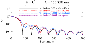
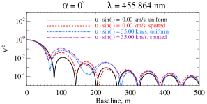
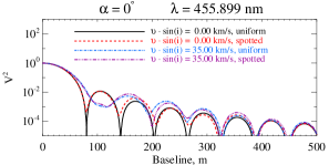
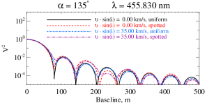
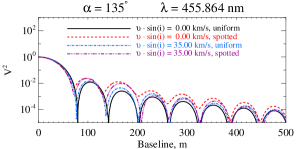
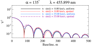
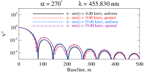
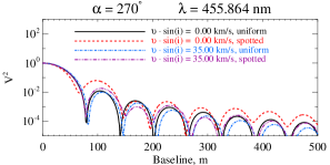
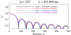
Figure 2: Stellar intensity images and squared visibility at three wavelengths (three columns from left to right) around Cr ii $455.86$ nm line and spectral resolution $R=30\,000$. The three images on top of each column show normalized intensity distributions of the star computed assuming (from left to right) $\upsilon\sin i=0$ km s^-1 with spots, $\upsilon\sin i=35$ km s^-1 without spots, and $\upsilon\sin i=35$ km s^-1 with spots, respectively. Three rows with squared visibility plots correspond to position angles of (from top to bottom) $0^{\circ}$, $135^{\circ}$, and $270^{\circ}$ respectively. Calculations are shown for the case of $\upsilon\sin i=0$ km s^-1 and $\upsilon\sin i=35$ km s^-1 for homogeneous and spotted stellar surfaces (see plot legends).

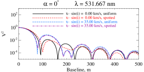
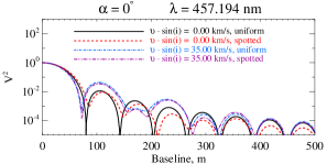
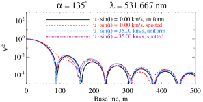
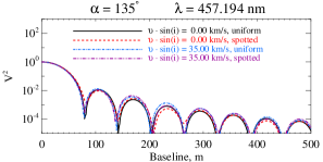
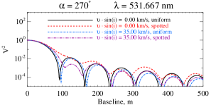
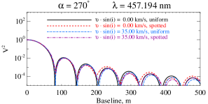
Figure 3: Same as on Fig. 2, but at the continuum wavelength $456.241$ nm, Fe ii $531.667$ nm, and a blend of Cr i$+$Ti 2 $457.194$ nm lines.

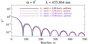
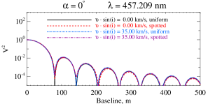
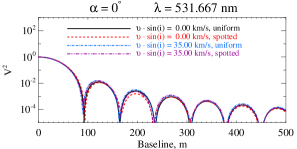
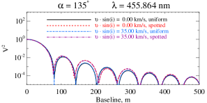
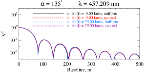
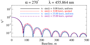
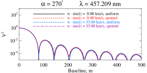
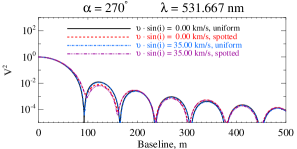
Figure 4: Same as on Fig. 2, but for Cr ii $455.86$ nm, blend of Cr i$+$Ti 2 lines at $457.194$ nm, and Fe ii $531.667$ nm line at spectral resolution $R=6\,000$.

4.1.2 Visibility vs. wavelength

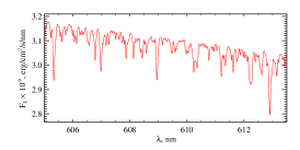
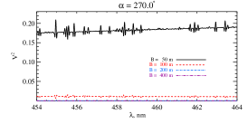
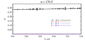
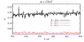
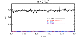
Figure 5: Squared visibility as a function of wavelength calculated at four selected baselines. First row – spectrum predicted by spotted model; second and third rows – squared visibility predicted by homogeneous and spotted models respectively. In all plots $R=30\,000$, $\upsilon\sin i=35$ km s^-1. Squared visibility plots show predictions for the orientation with position angle of $270^{\circ}$.

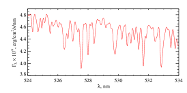
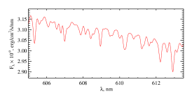
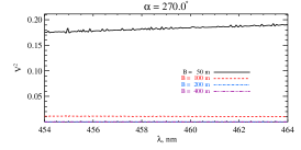
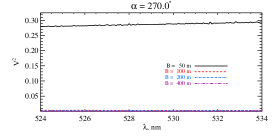
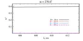
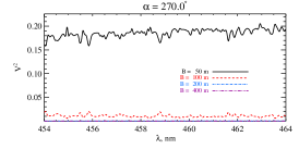
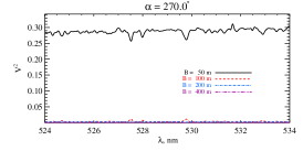
Figure 6: Same as on Fig. 5, but with $R=6\,000$.

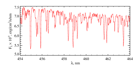
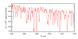
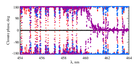
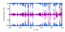
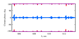
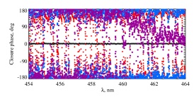
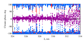
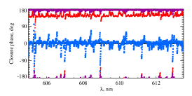
Figure 7: Closure phases as a function of wavelength. First row – spectrum predicted by spotted model; second and third rows – closure phase predicted by homogeneous and spotted models, respectively. In all plots $R=30\,000$, $\upsilon\sin i=35$ km s^-1. Closure phases were computed for the following configurations: ($0^{\circ},40$m)$+$($270^{\circ},40$m)$+$($135^{\circ},57$m) – black crosses; ($0^{\circ},100$m)$+$($270^{\circ},100$m)$+$($135^{\circ},141$m) – red diamonds; ($0^{\circ},180$m)$+$($270^{\circ},180$m)$+$($135^{\circ},255$m) – blue squares; ($0^{\circ},320$m)$+$($270^{\circ},320$m)$+$($135^{\circ},453$m) – violet circles. See online version for colored symbols.

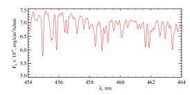
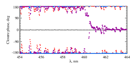
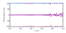
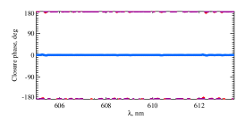
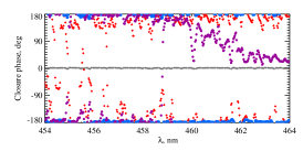
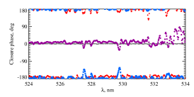
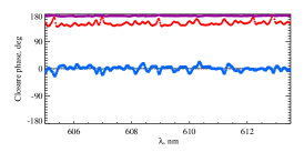
Figure 8: Same as on Fig. 7, but with $R=6\,000$. See online version for colored symbols.

First row of Fig. 5 illustrates the three wavelength intervals in visual domain that were used to compute wavelength dispersed squared visibility for $R=30\,000$. These visibilities are plotted in the second and third rows of Fig. 5 for the uniform and spotted surfaces and for $\upsilon\sin i=35$ km s^-1. As example, predictions only for $\alpha=270^{\circ}$ are shown because this configuration provides stronger signals compared with the other two. Features are observed at optical wavelengths while at longer wavelengths ($605.0-613.5$ nm) the intensity contrast become weaker and the signal amplitude drops significantly. By comparing visibility corresponding to star with and without spots, it is obvious that the presence of spots can be located already with short baselines ($\approx 50$ m, see the legend on Fig. 5).

At a lower spectral resolution of $R=6\,000$ rotation becomes less important and signals in $V^{2}$ are weak and rare, as shown in the Fig. 6. There are several deeps seen only for the spotted case at $454.0-464.0$ nm and $524.0-534.0$ nm regions, while only marginal features can be seen in the $605.0-613.5$ nm region.

4.1.3 Closure phase

To illustrate the closure phase signatures we assumed a simple isosceles triangle configuration of imaginary telescopes with two position angles of $0^{\circ}$ and $270^{\circ}$. Such a configuration implies that the third baseline must be oriented at $135^{\circ}$ and its length ($B_{\rm max}$ hereafter) is estimated from the $(u,v)$ coordinates of the first two projected baselines.

Figure 7 illustrates predictions for the same three spectral regions considered in the previous section, for uniform and spotted models, $R=30\,000$, and $\upsilon\sin i=35$ km s^-1. We find that at this resolution there is a clear signal in closure phase detected at maximum baseline of a triangle $B_{\rm max}>100$ m. However, at certain configurations it is indeed hard to see the difference between uniform and spotted stellar surfaces. Fortunately, there are many configurations for which the spotted star looks different compared to a homogeneous one. In general, a rotating star with uniform surface produces closure phases that are symmetric relative to the core of spectral lines, whereas spots induce more rich and complex closure phase patterns. Moreover, for a configuration with the sides of isosceles triangle of $100$ m and $200$ m (i.e. $B_{\rm max}=141$ m and $B_{\rm max}=255$ m, respectively) a clear spot signal is detected in $605.0-613.5$ nm spectral window where the rotation does not seem to affect the closure phase very much compared to the other two spectral regions of shorter wavelengths.

As already mentioned, at a lower spectral resolution of $R=6\,000$ rotation becomes less important and signals in closure phase are grossly due to spots, as shown on Fig. 8. Still, rotation is capable of inducing pretty strong features at several baselines and short wavelengths, but much more features are detected if star has spots. Similar to the previous case with $R=30\,000$, we find many configurations where the spot signals can be unambiguously detected.

In general, the spots are detected in all three wavelength windows, however at short wavelengths the spectral line density is higher and many signals are recovered. In case of very slow rotations, the short wavelengths will provide a rich and strong spot signals compared to longer wavelengths.

4.2 Infrared wavelength domain

4.2.1 Visibility vs. baseline

Hydrogen lines are the only strong spectroscopic features seen in infrared $J$, $H$, and $K$ bands. At $R=6\,000$ there are some lines of metals but their number decreases from towards longer wavelengths. As an example, on Fig. 9 we show model predictions at the cores of H, Fe, and Mg lines. Even in line cores the intensity contrast is weak. There is a clear yet small difference in squared visibility obtained at different position angles seen at baselines longer than a few hundred meters where squared visibility drops below $V^{2}\lesssim 10^{-2}$ in case of Fe and Mg lines, and nothing can be seen at the core of H line, at least above $V^{2}\geqslant 10^{-4}$.

4.2.2 Visibility vs. wavelength

Squared visibility computed at different spectral channels and resolutions $R=6\,000$ and $R=30$ are shown on Fig. 10. At both resolutions, squared visibility plots reveal no characteristic spectral line features except hydrogen lines and only with $R=6\,000$. At a lowest resolution of $R=30$ the spectral lines are not resolved, as shown in the third column of Fig. 10, and the uniform and spotted surface show very similar visibility curves.

4.2.3 Closure phase

The analysis of the closure phase signals demonstrate that the surface inhomogeneities can already be detected in the $J$ band between $1000$ nm and $1100$ nm, $R=6\,000$ and $B_{\rm max}>180$ m. An example of the strongest signal is shown in the left-hand column of Fig. 11 for $B_{\rm max}=184$ m. Spots are also detected at longer wavelengths. For instance, middle row of Fig. 11 illustrates predictions for a narrow spectral channel in $K$ band with a hydrogen line from Brackett series. Rotation signatures are visible at particular configurations, e.g. with $B_{\rm max}=184$ m in the $J$ band and $B_{\rm max}=506$ m in the $K$ band, but the shape of these signatures is strongly modified when spots are present.

There is no signal in closure phase seen for the homogeneous star at lowest resolution $R=30$. The spotted star also illustrates phase changes by $\pm 180^{\circ}$, but the closure phase pattern differs substantially from the homogeneous case: it does not show any sharp jumps but rather smooth transitions between $0^{\circ}$ and $180^{\circ}$. (see bottom left hand plot in Fig. 11). We therefore conclude that spots can be detected in infrared even with very low spectral resolution, but with baselines longer than $B_{\rm max}>180$ m.

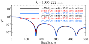
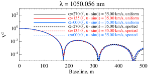
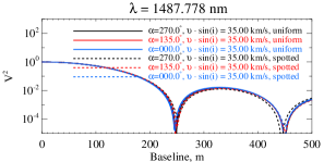
Figure 9: Squared visibility predicted at the cores of the H i $1005.2$ nm, Fe ii $1050.0$ nm, and Mg i $1487.7$ nm lines and spectral resolution $R=6\,000$. The rotational velocity is $\upsilon\sin i=35$ km s^-1. The squared visibility from homogeneous and spotted surfaces are shown by full and dashed lines respectively. Top panel shows intensity images with homogeneous and spotted abundance distributions.

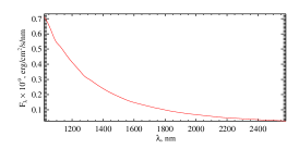
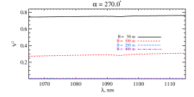
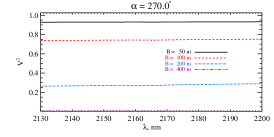
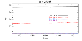
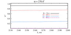
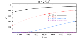
Figure 10: Squared visibility as a function of wavelength calculated at four selected baselines. First row – spectrum predicted by spotted model; second and third rows – squared visibility predicted by homogeneous and spotted models respectively. Three spectral windows are shown: $1065.0-1115.0$ nm, $R=6\,000$ (left column), $2130.0-2200.0$ nm, $R=6\,000$ (middle column), and $1020.0-2580.0$ nm, $R=30$ (right column). In all plots $\upsilon\sin i=35$ km s^-1.

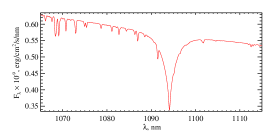
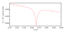
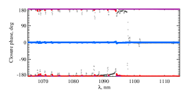
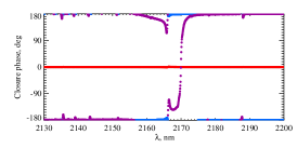
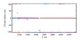
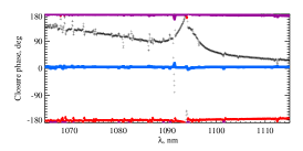
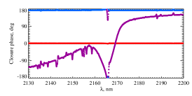
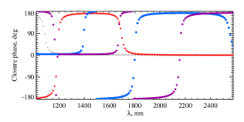
Figure 11: Closure phases as a function of wavelength. First row – spectrum predicted by spotted model; second and third rows – closure phase predicted by homogeneous and spotted models, respectively. Three spectral windows are shown: $1065.0-1115.0$ nm, $R=6\,000$ (left column), $2130.0-2200.0$ nm, $R=6\,000$ (middle column), and $1020.0-2580.0$ nm, $R=30$ (right column). In all plots $\upsilon\sin i=35$ km s^-1. Closure phases were computed for the following configurations: ($0^{\circ},130$m)$+$($270^{\circ},130$m)$+$($135^{\circ},184$m) – black crosses; ($0^{\circ},200$m)$+$($270^{\circ},200$m)$+$($135^{\circ},283$m) – red diamonds; ($0^{\circ},300$m)$+$($270^{\circ},300$m)$+$($135^{\circ},424$m) – blue squares; ($0^{\circ},358$m)$+$($270^{\circ},358$m)$+$($135^{\circ},506$m) – violet circles. See online version for colored symbols.

5 Discussion and conclusions

In this paper we examined the possibility to detect abundance spots in atmospheres of CP stars by running numerical simulations of such interferometric observable like visibility and closure phase. These quantities were computed at different wavelength domains and spectral resolutions. As a case study, we used abundance maps of the well-known CP star $\varepsilon$ UMa which has one of the largest angular diameter among all CP stars known by date.

We confirm that the best spectral regions to search for abundance spots and rotation are in the visual domain close to the Balmer jump, i.e. where the star radiates maximum of its flux. In that region, the intensity contrast is higher in spectral lines of spotted elements thus providing most easy way to detect and characterize them both from the analysis of squared visibility and closure phase. The spots and rotation signatures can also be detected in NIR. However, in our simulations this happens only at low squared visibility $V^{2}\leqslant 10^{-2}$ which corresponds to maximum baselines of triangle telescope configuration of $B_{\rm max}\geqslant 180$ m as seen in Fig. 11. Important that spots can be detected with very low spectral resolution of $R=30$ (see third column of Fig. 11). The stellar rotation is observed only if spectral lines, especially hydrogen lines (which are strongest spectral features in NIR), are resolved, i.e. with spectral resolution on the order of $R\sim 6\,000$ (see first and second columns of Fig. 11).

Because of star’s large angular diameter, its surface can already be resolved with relatively short baselines $B>50$ m in visual. Baselines longer than $B\gtrsim 200$ m are needed to resolve the star in infrared wavelengths.

Observing with high spectral resolution in visual domain allows one to constrain positions of abundance spots and stellar rotation velocity. To achieve this goal from squared visibility curves observations with different position angles are needed. The wavelength dispersed closure phases can also be used to derive stellar rotation and spots. This is possible because rotation induces a characteristic symmetric phase jump at both sides of cores of spectral lines (see, e.g., Fig. 7). When spots are presented, these signals are modified, as well as more features appear at other wavelengths.

The analysis of squared visibility shows that spots are clearly detected already at a first visibility lobe, at least in strong spectral features of such elements as Cr and Fe. Individual details depend on the position angle and, more critically, on spectral resolution (i.g. contrast). In most optimistic cases, the difference between spots and rotation becomes clearly noticeable at squared visibility $V^{2}\lesssim 0.3$ as shown using examples of Cr ii $455.86$ nm (Fig. 2) and Fe ii $531.67$ nm (Fig. 3) lines. From the behaviour of the position of the first visibility lobe we find that the effect of spots is to make the star look larger (compared to the spotless case) if spots are dark and smaller if spots are bright, respectively.

One of our goals was to verify whether the abundance inhomogeneities on the surface of $\varepsilon$ UMa can be detected with modern interferometric facilities. According to our simulations an instrument like VEGA or its successor based on the principle of the demonstrator FRIEND (Fibered and spectrally Resolved Interferometric Equipment New design, Bério et al. (2014)) should be able to detect the effect of spots and spots+rotation, provided that the instrument is able to measure squared visibility down to $\approx 10^{-3}$, and/or closure phase in visual. An instrument with the spectral resolution around $6\,000$ like AMBER or GRAVITY but baselines longer than $180$ m would be able to measure rotation, and also rotation+spots.

In Table LABEL:tab:stars we summarize the application of modern and planned interferometric facilities to a sample of CP stars. Majority of stars in this table are magnetic CP stars listed in Kochukhov & Bagnulo (2006) with four additional stars HD 37776, HD 72106, HD 103498, and HD 177410, and five presumably non-magnetic HgMn stars (shown in the end of the table). We used information from Table 1 to estimate the observability of each star as applied to a particular instrument. As seen from Table LABEL:tab:stars, for most of CP stars their estimated angular diameters are below $1$ mas. Therefore, both long baselines of hundreds of meters and detectors sensitive to values of $V^{2}<10^{-2}$ are required. One can see that there are many stars that cannot be observed with neither modern nor planned facilities. Such benchmark stars as, say, HD 101065 (Przybylski’s star) and HD 37776 (Landstreet’s star) are among them. On the other hand, we predict that it is possible to observe many stars with NPOI and/or SUSI if the baseline of the latter will be increased. This is the case for another well-known stars as, say, HD 137949 ($33$ Lib) and HD 65339 ($53$ Cam).

Finally, we find that a considerable fraction of CP stars in our sample can already be subject for spot detection using existing interferometric facilities. Magnetic stars HD 24712, HD 40312, HD 128898, HD 137909, HD 201601, as well as HgMn stars HD 358, HD 33904 are all well-known objects and for some of them DI maps are available in the literature. But there are many more in the table. Note that none of the stars from our sample can be observed with VLTI and the reason for this is a short baseline range provided by VLTI compared to other existing interferometers (see Table 1). In fact, among 203 stars listed in Table LABEL:tab:stars, 157 are visible at VLTI location, and several of them could be observed if VLTI had maximum baselines longer than $300$ m. Alternatively, there are two objects that could be observed already with available maximum baseline of $140$ m but detectors operating in visual were needed.

One should not forget that the brightness contrast in spectral lines that result from our simulations of $\varepsilon$ UMa may differ from the real one, at least at certain wavelengths. This may happen because of internal inaccuracies in atomic line parameters that affect the depth of respective spectroscopic features. This does not matter for the medium and low resolutions tested in our investigation, but may be an issue for the highest resolution of $R=30\,000$. We stress that observing with high resolution is important for studying the stratification of chemical elements over stellar surfaces and to constrain theoretical models because many features in visibility and closure phase can be studied.

A word of caution should be said regarding DI abundance maps themselves. In the DI code, the rotational modulation of spectral lines is interpreted as caused by abundance inhomogeneities only. In reality, however, other effects such as, say, magnetic fields (if not included in DI analysis), may also contribute to the absolute values of the surface abundances recovered (however, the relative abundance changes should not be affected much!). In case of $\varepsilon$ UMa the magnetic field is very weak, on the order of a few hundred Gauss (Wade et al. 2000), and thus cannot seriously affect the results of DI. Also, all modern DI codes map only horizontal distribution of chemical elements and ignore their vertical variations. This means that resulting abundance maps represent some vertically averaged abundance value. Nevertheless, modelling the light variability of $\varepsilon$ UMa Shulyak et al. (2010) obtained a good agreement between model predictions and observations based on the same DI maps that we used in this study. The authors, however, predicted the variability in narrow and broad-band photometric filters where the possible inaccuracies in atomic data and contrast in certain spectroscopic features, even if present, do not play critical role.

Finally, the above consideration also suggests that comparing the observed visibility with synthetic ones will allow us to constrain atmospheric models and to provide an independent validation of the DI results.

Table 2: Observability of CP stars with modern and future interferometers.

HD	$V$	$J$	$H$	$K$	$d$	$R$	$\theta$	$B_{\rm max}^{\dagger}$				ref.
number	mag	mag	mag	mag	pc	$R_{\odot}$	mas	m
								$0.55$ $\mu$m	$1.25$ $\mu$m	$1.65$ $\mu$m	$2.15$ $\mu$m
Magnetic CP stars
1048	6.25	6.14	6.24	6.22	140.8	2.37	0.16	723	1644	2170	2828	1
2453	6.91	6.71	6.76	6.74	221.7	2.57	0.11	1050	2388	3152	4108	1
3980	5.70	5.59	5.58	5.57	67.0	5.76	0.80	402	915	1208	1574	1
4778	6.15	6.09	6.15	6.14	100.3	1.91	0.18	641	1457	1923	2507	1
5737	4.27	4.63	4.81	4.67	238.1	7.52	0.29	385	877	1157	1508	1
8441	6.68	6.46	6.53	6.50	204.9	3.48	0.16	718	1632	2155	2808	1
9996	6.39	6.34	6.40	6.43	160.5	2.24	0.13	875	1989	2626	3422	1
10221	5.59	5.62	5.70	5.69	119.2	3.45	0.27	420	956	1262	1644	1
10783	6.43	6.54	6.58	6.56	176.7	3.17	0.17	679	1543	2037	2654	1
11187	7.94	7.13	7.22	7.23	321.5	2.92	0.08	1342	3051	4028	5249	1
11503	4.52	…	…	4.72	50.3	2.47	0.46	247	563	743	969	1
12288	7.74	7.42	7.40	7.43	308.6	2.55	0.08	1476	3355	4429	5771	1
12447	4.11	…	…	…	46.2	2.07	0.42	272	618	817	1064	1
12767	4.69	5.00	5.05	5.01	113.8	3.44	0.28	403	916	1210	1577	1
14437	7.27	7.26	7.29	7.31	159.7	2.46	0.14	792	1801	2378	3099	1
15089	4.53	…	…	…	40.7	2.13	0.49	233	529	699	911	1
15144	5.83	5.70	5.68	5.63	77.0	1.72	0.21	545	1238	1635	2130	1
17775	8.03	7.76	7.78	7.77	173.3	1.69	0.09	1249	2838	3747	4882	1
18296	5.10	5.11	5.24	5.23	98.0	3.77	0.36	317	720	951	1239	1
18610	8.14	7.89	7.95	7.88	213.2	2.53	0.11	1029	2339	3088	4024	1
19712	7.35	7.37	7.47	7.41	165.3	1.74	0.10	1156	2627	3468	4519	1
19805	7.96	7.69	7.70	7.66	222.2	1.87	0.08	1447	3289	4341	5657	1
19832	5.76	5.93	5.99	6.01	154.1	5.28	0.32	684	1556	2054	2676	1
21699	5.46	5.57	5.67	5.67	185.5	3.94	0.20	574	1305	1723	2245	1
22316	6.28	6.38	6.51	6.51	157.2	2.80	0.17	684	1555	2053	2675	1
22374	6.73	6.44	6.49	6.42	130.7	2.74	0.19	582	1323	1746	2276	1
22470	5.23	5.46	5.56	5.53	149.3	3.15	0.20	577	1312	1733	2258	1
22920	5.53	5.76	5.79	5.87	152.2	4.62	0.28	401	913	1205	1571	1
23207	7.54	7.27	7.29	7.25	207.0	2.64	0.12	956	2174	2870	3740	1
23408	3.87	3.93	4.12	3.99	117.5	5.76	0.46	248	565	746	972	1
24155	6.38	6.32	6.36	6.39	123.2	2.21	0.17	679	1544	2038	2656	1
24188	6.25	6.52	6.57	6.58	143.3	2.25	0.15	777	1767	2333	3040	1
24712	6.00	5.43	5.31	5.26	49.2	1.46	0.28	296	674	890	1160	1
25267	4.66	4.83	4.89	4.80	100.4	3.26	0.30	375	853	1126	1467	1
25354	7.84	7.78	7.87	7.82	155.3	1.49	0.09	1273	2893	3819	4976	1
25823	5.17	5.36	5.41	5.43	128.9	3.54	0.26	443	1008	1330	1733	1
27309	5.34	5.52	5.61	5.64	100.0	2.35	0.22	519	1181	1559	2031	1
28843	5.81	5.99	6.09	6.07	145.8	2.44	0.16	728	1655	2185	2847	1
30466	7.28	6.86	6.88	6.81	149.5	2.22	0.14	822	1870	2468	3216	1
32633	7.07	7.00	7.03	7.06	179.5	1.92	0.10	1142	2596	3428	4466	1
34452	5.37	5.63	5.75	5.76	126.7	2.81	0.21	550	1250	1651	2151	1
34797	6.54	6.70	6.80	6.77	244.5	3.35	0.13	891	2025	2674	3484	1
37776	6.96	7.29	7.42	7.42	330.0	2.75	0.08	1215	2762	3646	4751	2
38823	7.32	6.94	6.95	6.89	97.5	2.46	0.23	483	1099	1451	1891	1
39317	5.59	5.58	5.61	5.58	130.0	4.05	0.29	391	890	1174	1530	1
40312	2.62	2.69	2.70	2.75	50.8	4.58	0.84	148	336	444	578	1
42616	7.17	6.82	6.86	6.84	183.8	2.66	0.13	841	1913	2525	3290	1
42659	6.75	6.44	6.41	6.36	131.6	2.91	0.21	552	1254	1656	2157	1
49333	6.08	6.42	6.47	6.53	241.5	2.73	0.11	1078	2450	3235	4215	1
49976	6.29	6.25	6.27	6.23	99.9	2.00	0.19	610	1386	1830	2384	1
54118	5.17	5.26	5.32	5.29	92.3	2.66	0.27	423	962	1270	1655	1
55522	5.89	6.23	6.39	6.36	257.1	3.25	0.12	965	2194	2897	3774	1
55719	5.31	5.19	5.20	5.14	126.1	3.15	0.23	488	1109	1464	1908	1
56350	6.69	6.78	6.88	6.84	151.3	2.37	0.15	779	1770	2337	3045	1
60435	8.89	8.43	8.39	8.37	226.8	1.88	0.08	1473	3348	4420	5759	1
62140	6.47	6.16	6.18	6.17	96.7	2.09	0.20	563	1281	1691	2204	1
63401	6.25	6.56	6.66	6.68	200.4	3.09	0.14	790	1795	2370	3088	1
64486	5.39	…	…	…	99.0	2.89	0.27	418	950	1254	1635	1
64740	4.63	5.15	5.35	5.27	232.6	4.29	0.17	661	1502	1983	2584	1
65339	6.02	…	…	…	98.7	4.55	0.43	509	1157	1527	1990	1
71866	6.72	6.62	6.71	6.67	133.2	2.66	0.19	609	1385	1829	2383	1
72106	8.61	8.43	8.28	7.92	278.6	0.61	0.02	2560	5818	7680	10007	3
72968	5.72	5.71	5.75	5.69	92.9	2.04	0.20	555	1262	1666	2170	1
73340	5.78	6.02	6.03	6.04	136.8	2.62	0.18	636	1446	1909	2488	1
74521	5.66	5.72	5.79	5.82	129.7	3.00	0.22	526	1197	1580	2059	1
75445	7.12	6.64	6.52	6.53	108.3	2.18	0.19	606	1377	1818	2369	1
79158	5.29	5.41	5.53	5.53	178.3	4.21	0.22	516	1173	1548	2017	1
81009	6.53	6.22	6.24	6.15	144.5	2.71	0.17	649	1476	1948	2539	1
83368	6.23	…	…	…	70.6	2.35	0.31	429	977	1289	1680	1
83625	6.88	6.97	7.06	7.06	181.2	2.40	0.12	922	2095	2766	3605	1
86199	6.74	6.89	7.02	6.97	232.0	3.02	0.12	938	2132	2814	3667	1
88158	6.44	6.56	6.63	6.62	210.5	3.69	0.16	695	1579	2085	2717	1
88385	8.09	7.93	8.00	7.95	206.2	2.31	0.10	1089	2475	3267	4257	1
89103	7.78	7.97	8.08	8.06	188.7	1.66	0.08	1385	3148	4155	5414	1
90044	5.97	5.98	6.10	6.07	104.2	2.37	0.21	536	1219	1609	2096	1
90569	6.04	6.02	6.08	6.04	129.2	2.47	0.18	638	1450	1914	2495	1
92385	6.71	6.81	6.89	6.86	169.2	2.10	0.12	982	2232	2946	3839	1
92499	8.88	8.52	8.54	8.54	282.5	2.15	0.07	1602	3641	4807	6263	1
92664	5.52	5.79	5.87	5.88	160.5	2.84	0.16	689	1566	2067	2693	1
94427	7.36	6.72	6.62	6.55	143.5	2.19	0.14	797	1811	2391	3116	1
94660	6.11	6.21	6.17	6.20	149.9	2.81	0.17	649	1476	1948	2539	1
96707	6.08	5.57	5.53	5.50	111.2	3.22	0.27	421	958	1265	1648	1
98088	6.14	5.78	5.73	5.69	129.5	3.24	0.23	487	1108	1463	1906	1
98340	7.13	7.17	7.25	7.23	221.7	2.10	0.09	1287	2925	3861	5031	1
101065	8.03	7.11	6.94	6.92	112.0	1.98	0.16	689	1567	2069	2696	1
103192	4.28	4.36	4.56	4.43	95.0	3.94	0.39	294	668	882	1149	1
103498	6.99	6.81	6.87	6.86	296.7	4.50	0.14	804	1827	2412	3143	4
105382	4.47	4.82	4.95	4.87	134.4	3.35	0.23	490	1113	1470	1915	1
105770	7.37	7.02	7.03	6.96	191.2	2.53	0.12	921	2093	2763	3600	1
108662	5.24	5.22	5.30	5.29	72.9	2.43	0.31	365	829	1095	1427	1
108945	5.44	5.29	5.31	5.27	82.7	2.98	0.34	338	768	1015	1322	1
109026	3.88	4.20	4.25	4.25	99.6	4.24	0.40	286	651	859	1119	1
110066	6.40	6.29	6.33	6.33	134.6	3.19	0.22	513	1167	1541	2008	1
111133	6.34	6.28	6.34	6.33	266.0	3.09	0.11	1050	2388	3152	4108	1
112185	1.77	1.72	1.73	1.76	25.3	4.14	1.52	62	140	186	242	1
112381	6.49	…	…	…	118.5	1.66	0.13	869	1976	2609	3400	1
112413	2.88	3.05	3.13	3.16	35.2	3.42	0.91	186	424	560	730	1
115226	8.50	7.94	7.90	7.85	147.1	1.54	0.10	1164	2647	3494	4553	1
115440	8.24	8.04	8.04	8.03	199.2	1.91	0.09	1270	2888	3812	4967	1
115708	7.83	7.23	7.19	7.15	115.6	1.86	0.15	759	1727	2279	2970	1
116114	7.02	6.48	6.42	6.35	129.7	2.78	0.20	569	1295	1709	2227	1
116458	5.66	5.67	5.70	5.67	136.1	3.46	0.24	479	1089	1437	1873	1
116890	6.19	6.03	6.04	5.98	187.6	4.12	0.20	555	1263	1667	2173	1
117025	6.07	5.95	5.92	5.87	86.7	2.20	0.24	479	1089	1437	1873	1
118022	4.94	4.90	4.90	4.88	56.7	2.18	0.36	316	718	948	1236	1
118913	7.69	7.41	7.47	7.36	256.4	2.49	0.09	1255	2852	3765	4906	1
119213	6.29	6.15	6.21	6.20	91.1	1.96	0.20	567	1290	1703	2219	1
119308	7.86	7.75	7.79	7.76	245.1	1.76	0.07	1698	3860	5096	6640	1
119419	6.44	6.61	6.70	6.71	119.0	1.77	0.14	821	1866	2463	3210	1
120198	5.68	5.71	5.78	5.76	89.0	2.01	0.21	541	1230	1623	2115	1
122532	6.08	6.26	6.37	6.33	219.8	3.10	0.13	864	1964	2593	3379	1
122970	8.29	7.52	7.38	7.30	115.3	1.73	0.14	812	1846	2437	3175	1
124224	5.02	5.25	5.29	5.29	79.2	1.97	0.23	488	1111	1466	1911	1
125248	5.90	5.83	5.87	5.84	102.0	1.95	0.18	639	1452	1917	2498	1
125630	6.76	6.69	6.73	6.73	165.6	2.83	0.16	714	1622	2142	2791	1
125823	4.42	4.93	4.99	4.92	140.3	3.45	0.23	496	1127	1488	1939	1
126515	7.07	7.10	7.15	7.15	106.4	1.84	0.16	705	1603	2117	2758	1
127453	7.36	7.16	7.16	7.15	225.2	3.04	0.13	904	2055	2713	3535	1
127575	7.75	7.59	7.59	7.58	142.9	1.85	0.12	943	2144	2830	3687	1
128775	6.62	6.80	6.87	6.87	208.8	2.27	0.10	1120	2546	3361	4380	1
128898	3.19	2.84	2.73	2.74	16.6	1.94	1.09	104	236	312	407	1
129899	6.44	6.43	6.49	6.46	255.1	4.95	0.18	628	1429	1886	2457	1
130559	5.31	5.21	5.20	5.18	72.9	2.04	0.26	436	991	1308	1705	1
132322	7.37	6.97	7.01	6.90	196.1	2.75	0.13	869	1975	2608	3398	1
133029	6.35	6.49	6.58	6.57	169.8	2.51	0.14	825	1875	2476	3226	1
133652	5.97	6.04	6.07	6.05	121.4	1.83	0.14	808	1838	2426	3161	1
133792	6.25	6.02	6.07	6.00	181.5	3.85	0.20	574	1306	1724	2247	1
133880	5.79	5.99	5.91	5.99	110.7	2.51	0.21	537	1220	1611	2099	1
134214	7.46	6.82	6.68	6.67	102.7	1.71	0.15	733	1666	2199	2866	1
134305	7.25	6.81	6.79	6.75	150.6	2.93	0.18	626	1422	1878	2447	1
137509	6.87	7.02	7.13	7.18	195.7	2.81	0.13	847	1927	2543	3314	1
137909	3.68	3.38	3.28	3.28	34.3	2.47	0.67	169	384	507	661	1
137949	6.69	6.31	6.28	6.25	88.7	2.13	0.22	507	1153	1522	1984	1
138758	7.89	7.91	7.98	7.98	208.8	2.08	0.09	1225	2786	3677	4792	1
140160	5.33	5.18	5.23	5.20	67.4	2.25	0.31	365	829	1095	1426	1
140728	5.49	5.47	5.58	5.56	91.6	2.52	0.26	443	1007	1329	1732	1
142301	5.87	5.92	6.00	5.99	158.0	2.53	0.15	762	1733	2288	2981	1
142990	5.43	5.58	5.67	5.65	170.4	3.02	0.16	688	1565	2066	2692	1
143473	7.41	7.01	6.98	6.96	116.1	1.64	0.13	862	1960	2587	3371	1
144334	5.92	6.03	5.97	5.92	161.3	2.74	0.16	718	1632	2155	2808	1
145501	6.30	5.78	5.69	5.61	145.3	2.49	0.16	711	1617	2134	2781	1
147010	7.40	6.75	6.75	6.68	163.4	2.04	0.12	977	2221	2931	3820	1
148112	4.58	4.56	4.59	4.52	76.7	3.30	0.40	283	644	850	1108	1
148199	7.01	6.71	6.75	6.72	158.2	2.41	0.14	801	1822	2405	3134	1
148330	5.75	5.70	5.70	5.72	119.9	3.09	0.24	473	1076	1421	1852	1
149764	6.95	6.88	6.93	6.93	132.6	1.63	0.11	991	2253	2975	3876	1
149822	6.36	6.37	6.48	6.45	126.3	2.36	0.17	651	1481	1955	2547	1
149911	6.09	5.66	5.62	5.52	113.3	3.54	0.29	390	887	1172	1527	1
151525	5.24	5.08	5.08	5.10	120.6	4.86	0.37	302	688	908	1183	1
151965	6.33	6.51	6.60	6.60	180.5	2.54	0.13	865	1967	2596	3383	1
152107	4.82	4.78	4.58	4.57	55.2	2.27	0.38	296	673	889	1159	1
153882	6.31	6.14	6.16	6.16	162.9	3.53	0.20	563	1279	1689	2201	1
154708	8.76	8.11	7.98	7.95	148.1	1.70	0.11	1062	2415	3188	4154	1
157751	7.62	7.66	7.72	7.76	161.6	1.69	0.10	1167	2652	3501	4562	1
164258	6.37	5.93	5.89	5.89	135.3	2.85	0.20	579	1317	1738	2265	1
165474	7.50	…	…	…	138.1	2.23	0.15	755	1716	2265	2951	1
168733	5.34	5.53	5.56	5.58	170.6	4.54	0.25	458	1040	1374	1790	1
168856	7.05	6.59	6.61	6.55	190.8	2.38	0.12	978	2223	2934	3824	1
170000	4.22	4.18	4.45	4.39	92.9	3.53	0.35	321	729	963	1254	1
170397	6.03	5.94	5.96	5.93	104.8	1.83	0.16	698	1587	2095	2730	1
171184	7.89	7.29	7.28	7.23	222.2	2.30	0.10	1179	2679	3537	4609	1
171586	6.46	6.23	6.31	6.29	110.3	2.14	0.18	629	1431	1889	2461	1
172690	7.49	7.40	7.47	7.43	280.1	2.71	0.09	1262	2868	3786	4933	1
173650	6.52	6.38	6.43	6.40	215.5	3.92	0.17	670	1523	2010	2620	1
175132	6.27	6.32	6.37	6.38	492.6	6.99	0.13	859	1953	2578	3360	1
175362	5.38	5.62	5.66	5.68	131.9	2.57	0.18	626	1424	1880	2450	1
176196	7.51	7.56	7.62	7.58	222.2	2.68	0.11	1010	2296	3031	3950	1
176232	5.89	5.42	5.32	5.30	78.4	2.43	0.29	393	894	1180	1538	1
177410	6.50	6.75	6.83	6.88	213.2	2.68	0.12	1061	2413	3185	4150	5
179527	5.93	5.90	6.00	6.00	273.2	6.40	0.22	520	1182	1561	2034	1
183056	5.15	5.30	5.43	5.44	216.9	5.03	0.22	526	1195	1578	2056	1
183339	6.58	6.88	6.99	6.97	361.0	4.80	0.12	916	2083	2750	3584	1
183806	5.58	5.56	5.61	5.53	121.7	3.61	0.28	411	934	1233	1606	1
184905	6.62	6.63	6.70	6.72	189.0	2.62	0.13	879	1999	2639	3438	1
187474	5.33	5.37	5.44	5.43	92.4	2.85	0.29	394	897	1184	1543	1
188041	5.63	5.53	5.55	5.49	80.1	2.80	0.32	349	794	1048	1366	1
192678	7.34	7.24	7.32	7.33	198.0	2.85	0.13	848	1927	2544	3315	1
196178	5.77	…	…	…	132.3	2.80	0.20	577	1311	1731	2255	1
196502	5.19	5.20	5.06	5.03	121.4	4.32	0.33	342	778	1027	1339	1
199728	6.25	6.40	6.45	6.47	164.2	2.15	0.12	931	2116	2794	3641	1
200177	7.34	7.21	7.27	7.26	159.0	1.72	0.10	1130	2568	3390	4417	1
201018	8.63	…	…	…	152.4	1.35	0.08	1373	3121	4120	5369	1
201601	4.68	4.28	4.18	4.10	36.3	2.07	0.53	213	486	641	835	1
203006	4.82	4.73	4.70	4.71	60.5	2.02	0.31	364	829	1094	1426	1
204411	5.31	5.05	5.08	5.06	126.1	4.12	0.30	373	849	1121	1460	1
205087	6.68	6.72	6.82	6.83	170.4	2.80	0.15	741	1685	2224	2898	1
208217	7.19	6.93	6.94	6.84	139.5	2.29	0.15	741	1685	2225	2899	1
212385	6.84	6.67	6.69	6.63	126.3	2.03	0.15	758	1724	2276	2965	1
215038	8.15	8.14	8.16	8.20	317.5	1.96	0.06	1979	4497	5937	7736	1
216018	7.62	7.34	7.37	7.31	124.5	1.53	0.11	990	2252	2972	3873	1
217522	7.52	6.79	6.69	6.63	88.0	2.07	0.22	518	1177	1554	2025	1
217833	6.52	6.54	6.62	6.63	260.4	3.00	0.11	1060	2409	3181	4144	1
220825	4.94	4.92	4.97	4.96	47.1	1.92	0.38	299	680	898	1170	1
221006	5.68	5.92	6.03	6.00	118.5	2.23	0.18	647	1472	1943	2532	1
221394	6.41	6.26	6.32	6.31	129.0	2.85	0.21	551	1253	1654	2155	1
221568	7.55	7.43	7.48	7.48	217.4	3.31	0.14	801	1822	2405	3133	1
223640	5.18	5.42	5.51	5.50	97.8	2.57	0.24	463	1053	1390	1811	1
224801	6.35	6.41	6.51	6.51	188.0	3.49	0.17	657	1494	1972	2570	1
HgMn stars
358	2.06	2.30	2.33	2.37	29.7	2.48	0.78	142	323	427	556	6
11753	5.11	5.17	5.25	5.17	94.1	9.50	0.94	407	926	1222	1593	7
32964	5.12	5.23	5.22	5.20	94.7	2.40	0.24	597	1358	1793	2336	8
33904	3.29	3.53	3.59	3.57	57.0	3.39	0.55	205	466	615	801	9
34364	6.14	6.19	6.25	6.26	122.1	3.70	0.28	788	1792	2366	3083	10

Table 2: continued.

References

- Adelman et al. (2002) Adelman, S. J., Gulliver, A. F., Kochukhov, O. P., & Ryabchikova, T. A. 2002, ApJ, 575, 449
- Asplund et al. (2009) Asplund, M., Grevesse, N., Sauval, A. J., & Scott, P. 2009, ARA&A, 47, 481
- Bério et al. (2014) Bério, Ph., Bresson, Y., Clausse, J.-M., et al. 2014, SPIE, Conf. 9146
- Boyajian et al. (2013) Boyajian, T. S., von Braun, K., van Belle, G., et al. 2013, ApJ, 771, 40
- Bruntt et al. (2010) Bruntt, H., Kervella, P., Mérand, A., et al. 2010, A&A, 512, A55
- Bruntt et al. (2008) Bruntt, H., North, J. R., Cunha, M., et al. 2008, MNRAS, 386, 2039
- Che et al. (2011) Che, X., Monnier, J. D., Zhao, M., et al. 2011, ApJ, 732, 68
- Chiavassa et al. (2010) Chiavassa, A., Lacour, S., Millour, F., et al. 2010, A&A, 511, A51
- Deutsch (1958) Deutsch, A. J. 1958, Electromagnetic Phenomena in Cosmical Physics, 6, 209
- Eisenhauer et al. (2008) Eisenhauer, F., Perrin, G., Brandner, W., et al. 2008, Proc. SPIE, 7013,
- Folsom et al. (2010) Folsom, C. P., Kochukhov, O., Wade, G. A., Silvester, J., & Bagnulo, S. 2010, MNRAS, 407, 2383
- Folsom et al. (2008) Folsom, C. P., Wade, G. A., Kochukhov, O., et al. 2008, Contributions of the Astronomical Observatory Skalnate Pleso, 38, 245
- Freyhammer et al. (2008) Freyhammer, L. M., Elkin, V. G., Kurtz, D. W., Mathys, G., & Martinez, P. 2008, MNRAS, 389, 441
- Ghasempour et al. (2012) Ghasempour, A., Muterspaugh, M., Hutter, D., et al. 2012, American Astronomical Society Meeting Abstracts #219, 219, #446.13
- Goncharskii et al. (1977) Goncharskii, A. V., Stepanov, V. V., Kokhlova, V. L., & Yagola, A. G. 1977, Soviet Astronomy Letters, 3, 147
- Ireland et al. (2008) Ireland, M. J., Mérand, A., ten Brummelaar, T. A., et al. 2008, Proc. SPIE, 7013,
- Khan & Shulyak (2007) Khan, S. A., & Shulyak, D. V. 2007, A&A, 469, 1083
- Khokhlova et al. (2000) Khokhlova, V. L., Vasilchenko, D. V., Stepanov, V. V., & Romanyuk, I. I. 2000, Astronomy Letters, 26, 177
- Kochukhov et al. (2011) Kochukhov, O., Makaganiuk, V., Piskunov, N., et al. 2011, A&A, 534, L13
- Kochukhov & Bagnulo (2006) Kochukhov, O., & Bagnulo, S. 2006, A&A, 450, 763
- Kochukhov et al. (2005) Kochukhov, O., Piskunov, N., Sachkov, M., & Kudryavtsev, D. 2005, A&A, 439, 1093
- Kochukhov et al. (2004) Kochukhov, O., Drake, N. A., Piskunov, N., & de la Reza, R. 2004, A&A, 424, 935
- Kochukhov & Ryabchikova (2001) Kochukhov, O., & Ryabchikova, T. 2001, A&A, 377, L22
- Krtička et al. (2012) Krtička, J., Mikulášek, Z., Lüftinger, T., et al. 2012, A&A, 537, A14
- Krtička et al. (2009) Krtička, J., Mikulášek, Z., Henry, G. W., et al. 2009, A&A, 499, 567
- Krtička et al. (2007) Krtička, J., Mikulášek, Z., Zverko, J., & Žižńovský, J. 2007, A&A, 470, 1089
- Kupka et al. (1999) Kupka, F., Piskunov, N., Ryabchikova, T. A., Stempels, H. C., & Weiss, W. W. 1999, A&AS, 138, 119
- Le Bouquin et al. (2011) Le Bouquin, J.-B., Berger, J.-P., Lazareff, B., et al. 2011, A&A, 535, A67
- Le Bouquin et al. (2009) Le Bouquin, J.-B., Lacour, S., Renard, S., et al. 2009, A&A, 496, L1
- Lemke (1997) Lemke, M. 1997, A&AS, 122, 285
- Li Causi (2008) Li Causi, G. 2008, Proc. SPIE, 7013,
- Lüftinger et al. (2010) Lüftinger, T., Fröhlich, H.-E., Weiss, W. W., et al. 2010, A&A, 509, A43
- Lueftinger et al. (2003) Lueftinger, T., Kuschnig, R., Piskunov, N. E., & Weiss, W. W. 2003, A&A, 406, 1033
- Maestro et al. (2013) Maestro, V., Che, X., Huber, D., et al. 2013, MNRAS, 434, 1321
- Makaganiuk et al. (2012) Makaganiuk, V., Kochukhov, O., Piskunov, N., et al. 2012, A&A, 539, A142
- Makaganiuk et al. (2011) Makaganiuk, V., Kochukhov, O., Piskunov, N., et al. 2011, A&A, 529, A160
- Mashonkina et al. (2009) Mashonkina, L., Ryabchikova, T., Ryabtsev, A., & Kildiyarova, R. 2009, A&A, 495, 297
- Mazumdar et al. (2009) Mazumdar, A., Mérand, A., Demarque, P., et al. 2009, A&A, 503, 521
- Michaud (1970) Michaud, G. 1970, ApJ, 160, 641
- Monnier et al. (2012) Monnier, J. D., Che, X., Zhao, M., et al. 2012, ApJ, 761, L3
- Monnier et al. (2007) Monnier, J. D., Zhao, M., Pedretti, E., et al. 2007, Science, 317, 342
- Monnier et al. (2004) Monnier, J. D., Berger, J.-P., Millan-Gabet, R., & ten Brummelaar, T. A. 2004, Proc. SPIE, 5491, 1370
- Montarges et al. (2014) Montarges et al., 2014, in prep.
- Mourard et al. (2011) Mourard, D., Bério, P., Perraut, K., et al. 2011, A&A, 531, A110
- Mourard et al. (2009) Mourard, D., Clausse, J. M., Marcotto, A., et al. 2009, A&A, 508, 1073
- O’Brien et al. (2011) O’Brien, D. P., McAlister, H. A., Raghavan, D., et al. 2011, ApJ, 728, 111
- Ohnaka et al. (2009) Ohnaka, K., Hofmann, K.-H., Benisty, M., et al. 2009, A&A, 503, 183
- Pandey et al. (2011) Pandey, C. P., Shulyak, D. V., Ryabchikova, T., & Kochukhov, O. 2011, MNRAS, 417, 444
- Petrov et al. (2007) Petrov, R. G., Malbet, F., Weigelt, G., et al. 2007, A&A, 464, 1
- Piskunov et al. (1995) Piskunov, N. E., Kupka, F., Ryabchikova, T. A., Weiss, W. W., & Jeffery, C. S. 1995, A&AS, 112, 525
- Piskunov & Rice (1993) Piskunov, N. E., & Rice, J. B. 1993, PASP, 105, 1415
- Perraut et al. (2013) Perraut, K., Borgniet, S., Cunha, M., et al. 2013, A&A, 559, A21
- Perraut et al. (2011) Perraut, K., Brandão, I., Mourard, D., et al. 2011, A&A, 526, A89
- Ryabchikova et al. (2004) Ryabchikova, T., Nesvacil, N., Weiss, W. W., Kochukhov, O., & Stütz, C. 2004, A&A, 423, 705
- Ryabchikova et al. (1999) Ryabchikova, T. A., Malanushenko, V. P., & Adelman, S. J. 1999, A&A, 351, 963
- Rousselet-Perraut et al. (2004) Rousselet-Perraut, K., Stehlé, C., Lanz, T., et al. 2004, A&A, 422, 193
- Scott et al. (2013) Scott, N. J., Millan-Gabet, R., Lhomé, E., et al. 2013, Journal of Astronomical Instrumentation , 2, 40005
- Ten Brummelaar et al. (2013) Ten Brummelaar, T. A., Sturmann, J., Ridgway, S. T., et al. 2013, Journal of Astronomical Instrumentation , 2, 40004
- Shulyak et al. (2010) Shulyak, D., Krtička, J., Mikulášek, Z., Kochukhov, O., Lüftinger, T. 2010, A&A, 524, A66
- Shulyak et al. (2004) Shulyak, D., Tsymbal, V., Ryabchikova, T., Stütz, C., & Weiss, W. W. 2004, A&A, 428, 993
- Vidal et al. (1973) Vidal, C. R., Cooper, J., & Smith, E. W. 1973, ApJS, 25, 37
- Wade et al. (2000) Wade, G. A., Donati, J.-F., Landstreet, J. D., & Shorlin, S. L. S. 2000, MNRAS, 313, 851
- Zhao et al. (2009) Zhao, M., Monnier, J. D., Pedretti, E., et al. 2009, ApJ, 701, 209