Metallicity of M dwarfs

Abstract

Aims. In this work we develop a technique to obtain high precision determinations of both metallicity and effective temperature of M dwarfs in the optical.

Methods. A new method is presented that makes use of the information of 4104 lines in the 530-690 nm spectral region. It consists in the measurement of pseudo equivalent widths and their correlation with established scales of [Fe/H] and $T_{eff}$.

Results. Our technique achieves a $rms$ of 0.08$\pm$0.01 for [Fe/H], 91$\pm$13 K for $T_{eff}$, and is valid in the (-0.85, 0.26 dex), (2800, 4100 K), and (M0.0, M5.0) intervals for [Fe/H], $T_{eff}$ and spectral type respectively. We also calculated the RMSE_V which estimates uncertainties of the order of 0.12 dex for the metallicity and of 293 K for the effective temperature. The technique has an activity limit and should only be used for stars with $\log{L_{H_{\alpha}}/L_{bol}}<-4.0$. Our method is available online at http://www.astro.up.pt/resources/mcal.

1 Introduction

The precise derivation of M dwarf atmospheric parameters is still very challenging today. Cool and intrinsically faint, M dwarfs are not easy to study. As the M subtype increases more molecules form in their atmosphere, making the spectral continuum very hard or impossible to identify, at least in the visible region of the spectrum. Therefore, methods such as atomic line analysis that are dependent on the knowledge of the continuum are suited only for the metal poor and earliest types of M dwarfs (e.g. Woolf & Wallerstein 2005, 2006). On the other hand, spectral synthesis techniques do not reach yet a high precision comparable to FGK dwarf methods, due to the fundamental lack of knowledge of billions of molecular line strengths and transitions, and most studies have reached modest results (e.g. Valenti et al. 1998; Bean et al. 2006). Despite that, some important progress have been made using spectral synthesis fitting to high-resolution spectra in the infrared (Önehag et al. 2012), where the depression of the continuum in some regions is less intense than in the visible region of the spectrum (e.g. Rajpurohit et al. 2013b). However, only a few stars have been measured this way, and the technique lacks external confirmation. An alternative method, based on high-resolution template spectra, to calculate metallicity, distance, stellar mass, and radius, was presented by (Pineda et al. 2013). This new technique, with similarities with our own method (Neves et al. 2013), is very promising but its [Fe/H] precision is still limited to 0.15 dex.

In this context, most parameter determinations, especially metallicity and effective temperature are instead based on calibrations using colours (e.g. Bonfils et al. 2005; Johnson & Apps 2009; Schlaufman & Laughlin 2010; Johnson et al. 2012; Neves et al. 2012) or spectroscopic indices (e.g. Rojas-Ayala et al. 2010, 2012; Mann et al. 2013a, b; Newton 2013).

Regarding metallicity, some progress has been made in the last few years. A steady improvement was achieved, bringing the typical uncertainties of $\pm$ 0.20 dex of the photometric calibrations, below $\sim 0.10$ dex in the most recent low-resolution spectroscopic scales in the infrared (e.g. Rojas-Ayala et al. 2012; Mann et al. 2013a; Newton 2013), following the pioneering work of Rojas-Ayala et al. (2010). However a true high-precision determination with a rms of the order of 0.05 dex, on par with the ones obtained for FGK dwarfs (e.g. Santos et al. 2004; Sousa et al. 2007) has not yet been reached (see Neves et al. (2012) introduction).

For temperature, on the other hand, important uncertainties and systematics still persist today. Although internal precisions are reported to be lower than 100K (e.g. Casagrande et al. 2008; Rojas-Ayala et al. 2012; Boyajian et al. 2012), their suffer from systematics ranging from 150 to 300 K making the determination of accurate temperature for M dwarfs a priority. In this context Boyajian et al. (2012) presented several calibrations of $T_{eff}$, based on the largest sample to date of high precision interferometric measurements of K and M dwarf radii and bolometric fluxes, that in principle allow a very precise measurement of the effective temperature (a technique pioneered by Ségransan et al. (2003) for M dwarfs). However, some doubts still arise regarding the accuracy of the determination of the total flux of the stars, based on templates from Pickles (1998), as recently pointed out by Mann et al. (2013b). They have, in turn, also recently presented their own effective temperature method that is very similar to the one of Boyajian et al. (2012) but rely on a combination of their low resolution spectra with BT-SETTL synthetic spectra from Allard et al. (2011, 2013) to calculate the bolometric flux. From these high-precision effective temperatures they established four visual and infrared spectroscopic indices, with precisions (but not accuracies) between 62 and 100 K. A similar effort regarding $T_{eff}$ determination of M dwarfs using synthetic spectra came from Rajpurohit et al. (2013a), where they compare synthetic spectra from the latest BT-SETTL models (Allard et al. 2012) to low-resolution optical spectra. They obtain a better agreement between synthetic and observed spectra when compared with previous models, estimating uncertainties of $T_{eff}$ of the order of 100 K.

In this work we present a new method to try to overcome the aforementioned hurdles and improve on the precision of both metallicity and effective temperature of M dwarfs. An early version of this new technique was briefly presented in the Appendix of Neves et al. (2013) and used to investigate the planet-metallicity relation of the HARPS GTO M dwarf sample (Bonfils et al. 2013). In Sect. 2 we describe in detail our method, as well as the sample selection, uncertainty estimation and a test of the technique as a function of resolution and signal-to-noise ratio (S/N). Afterwards, in Sect. 3, we compare our results with other determinations from the literature. Finally, in Sect 4 we discuss our results. The instructions to use our method are described in the Appendix.

2 The method

Our new method is based on the measurement of pseudo equivalent widths (EWs) of most lines/features in the 530-690 nm region of the spectra from a 102 star sample from the HARPS GTO M dwarf program, described in detail in Sect. 2 of Bonfils et al. (2013). It is a volume-limited sample (11 pc), and contains stars with $\delta<+20^{\circ}$, $V<14$ mag and includes only targets with $vsini\leq 6.5$ km/s. Spectroscopic binaries as well as visual pairs with separations lower than 5$\arcsec$ were removed a priori.

The features are defined as regions of the spectra that are formed by more than one line. The EWs are then correlated with the reference photometric [Fe/H] and $T_{eff}$ scales from Neves et al. (2012) and Casagrande et al. (2008) respectively. The two scales are in turn based on [Fe/H] determinations from FGK primaries with a M dwarf secondary and on an adaptation of the IRFM technique (Blackwell & Shallis 1977) respectively.

This method achieves an increase in precision of both parameters whereas its accuracy is tied to the original calibrations. The methodology is detailed in Sect. 2.1.

The reference [Fe/H] was calculated using stellar parallaxes, $V$, and $K_{S}$ magnitudes following the procedure described in Neves et al. (2012). The reference $T_{eff}$ is the average value of the $V-J$, $V-H$, and $V-K$ photometric scales taken from Casagrande et al. (2008). Table 1 lists the quantities used to calculate these parameters. Column 1 shows the star name, column 2 and 3 the right ascension and declination respectively, column 4 the parallax of each star and its associated error, and column 5 the source of the parallax measurement. Column 6 depicts the stellar type of the star taken from Simbad (Wenger et al. 2000), except in the case of Gl438, where it was obtained from Hawley et al. (1997). The photometric stellar type presented in Column 7 was calculated with the color relation of Lépine et al. (2013), and columns 8 to 11 display the $V$, $J$, $H$, and $K_{S}$ photometry. Lastly, column 12 details the source of the photometry.

Table 1: List containing our sample and the quantities used to calculate the reference [Fe/H] and T_eff . Sorted by right ascension.

star	$\alpha(2000)$	$\delta(2000)$	$\pi$	$\pi$	Stype	Stype	V	J	H	K	V/J/H/K
			[mas]	source	(S)	Phot.	[mag]	[mag]	[mag]	[mag]	source
Gl1	00:05:25	-37:21:23	$230.4\pm 0.9$	H	M1.5	M1.5	$8.56\pm 0.02$	$5.34\pm 0.02$	$4.73\pm 0.02$	$4.54\pm 0.02$	1/1/1/1
Gl54.1	01:12:31	-17:00:00	$271.0\pm 8.4$	H	M4Ve	M4.0	$12.07\pm 0.02$	$7.26\pm 0.02$	$6.75\pm 0.03$	$6.42\pm 0.02$	1/8/8/8
Gl87	02:12:21	+03:34:30	$96.0\pm 1.7$	H	M2.5V	M1.5	$10.04\pm 0.02$	$6.83\pm 0.02$	$6.32\pm 0.03$	$6.08\pm 0.02$	1/8/8/8
Gl105B	02:36:16	+06:52:12	$139.3\pm 0.5$	H	M4.5V	M3.5	$11.66\pm 0.02$	$7.33\pm 0.02$	$6.79\pm 0.04$	$6.57\pm 0.02$	4/8/8/8
HIP12961	02:46:43	-23:05:12	$43.5\pm 1.7$	H	M0	-	$10.24\pm 0.02$	$7.56\pm 0.02$	$6.93\pm 0.03$	$6.74\pm 0.02$	1/8/8/8
LP771-95A	03:01:51	-16:35:36	$146.4\pm 2.9$	H06	M3.5	M2.0	$10.59\pm 0.05$	$7.11\pm 0.02$	$6.56\pm 0.02$	$6.29\pm 0.02$	2/8/8/8
GJ163	04:09:16	-53:22:25	$66.7\pm 1.8$	H	M3.5	M3.0	$11.81\pm 0.02$	$7.95\pm 0.03$	$7.43\pm 0.04$	$7.13\pm 0.02$	1/8/8/8
Gl176	04:42:56	+18:57:29	$106.2\pm 2.5$	H	M2	M2.0	$9.95\pm 0.02$	$6.46\pm 0.02$	$5.82\pm 0.03$	$5.61\pm 0.03$	1/8/8/8
GJ179	04:52:06	+06:28:36	$81.4\pm 4.0$	H	M3.5	M3.5	$12.02\pm 0.04$	$7.81\pm 0.02$	$7.21\pm 0.05$	$6.94\pm 0.02$	1/8/8/8
Gl191	05:11:40	-45:01:06	$255.3\pm 0.9$	H	sdM1.0	M0.5	$8.85\pm 0.02$	$5.82\pm 0.03$	$5.32\pm 0.03$	$5.05\pm 0.02$	1/8/8/8
Gl205	05:31:27	-03:40:42	$176.8\pm 1.2$	H	M1.5V	M1.5	$7.97\pm 0.02$	$4.75\pm 0.05$	$4.07\pm 0.05$	$3.85\pm 0.03$	1/9/9/9
Gl213	05:42:09	+12:29:23	$171.6\pm 4.0$	H	M4.0V	M4.0	$11.56\pm 0.01$	$7.12\pm 0.02$	$6.63\pm 0.02$	$6.39\pm 0.02$	3/8/8/8
Gl229	06:10:34	-21:51:53	$173.8\pm 1.0$	H	M1/M2V	M1.0	$8.12\pm 0.02$	$5.06\pm 0.02$	$4.36\pm 0.02$	$4.16\pm 0.02$	1/1/1/1
HIP31293	06:33:43	-75:37:47	$110.9\pm 2.2$	H	M2V	M2.5	$10.35\pm 0.01$	$6.72\pm 0.02$	$6.15\pm 0.03$	$5.86\pm 0.02$	3/8/8/8
HIP31292	06:33:47	-75:37:30	$114.5\pm 3.2$	H	M3V	M3.0	$11.41\pm 0.01$	$7.41\pm 0.03$	$6.85\pm 0.03$	$6.56\pm 0.02$	3/8/8/8
Gl250B	06:52:18	-05:11:24	$114.8\pm 0.4$	H	M2	M2.0	$10.08\pm 0.01$	$6.58\pm 0.03$	$5.98\pm 0.06$	$5.72\pm 0.04$	5/8/8/8
Gl273	07:27:24	+05:13:30	$263.0\pm 1.4$	H	M3.5V	M3.5	$9.87\pm 0.02$	$5.71\pm 0.03$	$5.22\pm 0.06$	$4.86\pm 0.02$	1/8/8/8
Gl300	08:12:41	-21:33:12	$125.8\pm 1.0$	H	M4	M4.0	$12.13\pm 0.01$	$7.60\pm 0.02$	$6.96\pm 0.03$	$6.71\pm 0.03$	2/8/8/8
GJ2066	08:16:08	+01:18:11	$109.6\pm 1.5$	H	M2.0V	M2.0	$10.09\pm 0.02$	$6.62\pm 0.03$	$6.04\pm 0.03$	$5.77\pm 0.02$	1/8/8/8
GJ317	08:40:59	-23:27:23	$65.3\pm 0.4$	A12	M3.5	M3.0	$11.97\pm 0.04$	$7.93\pm 0.03$	$7.32\pm 0.07$	$7.03\pm 0.02$	2/8/8/8
Gl341	09:21:38	-60:16:53	$95.6\pm 0.9$	H	M0.0	M0.5	$9.46\pm 0.02$	$6.44\pm 0.02$	$5.79\pm 0.03$	$5.59\pm 0.02$	1/8/8/8
GJ1125	09:30:44	+00:19:18	$103.5\pm 3.9$	H	M3.5	M3.0	$11.71\pm 0.02$	$7.70\pm 0.02$	$7.18\pm 0.03$	$6.87\pm 0.02$	1/8/8/8
Gl357	09:36:02	-21:39:42	$110.8\pm 1.9$	H	M2.5V	M2.5	$10.91\pm 0.02$	$7.34\pm 0.03$	$6.74\pm 0.03$	$6.47\pm 0.02$	1/8/8/8
Gl358	09:39:47	-41:04:00	$105.6\pm 1.6$	H	M3	M3.0	$10.69\pm 0.02$	$6.90\pm 0.03$	$6.32\pm 0.05$	$6.06\pm 0.02$	1/8/8/8
Gl367	09:44:30	-45:46:36	$101.3\pm 3.2$	H	M1.0	M1.5	$9.98\pm 0.02$	$6.63\pm 0.02$	$6.04\pm 0.04$	$5.78\pm 0.02$	1/8/8/8
Gl382	10:12:17	-03:44:47	$127.1\pm 1.9$	H	M2.0V	M2.0	$9.26\pm 0.02$	$5.89\pm 0.02$	$5.26\pm 0.02$	$5.01\pm 0.02$	1/8/8/8
Gl393	10:28:55	+00:50:23	$141.5\pm 2.2$	H	M2.5V	M2.0	$9.63\pm 0.02$	$6.18\pm 0.02$	$5.61\pm 0.03$	$5.31\pm 0.02$	1/8/8/8
GJ3634	10:58:35	-31:08:38	$50.5\pm 1.6$	R10	M2.5	M2.5	$11.93\pm 0.02$	$8.36\pm 0.02$	$7.76\pm 0.05$	$7.47\pm 0.03$	2/8/8/8
Gl413.1	11:09:31	-24:36:00	$93.0\pm 1.7$	H	M2	M2.0	$10.45\pm 0.02$	$6.95\pm 0.02$	$6.36\pm 0.04$	$6.10\pm 0.02$	1/8/8/8
Gl433	11:35:27	-32:32:23	$112.6\pm 1.4$	H	M1.5	M1.5	$9.81\pm 0.02$	$6.47\pm 0.02$	$5.86\pm 0.04$	$5.62\pm 0.02$	1/8/8/8
Gl436	11:42:11	+26:42:23	$98.6\pm 2.3$	H	M3.5V	M2.5	$10.61\pm 0.01$	$6.90\pm 0.02$	$6.32\pm 0.02$	$6.07\pm 0.02$	2/8/8/8
Gl438	11:43:20	-51:50:23	$91.7\pm 2.0$	R10	M0.0†	M1.5	$10.36\pm 0.04$	$7.14\pm 0.02$	$6.58\pm 0.04$	$6.32\pm 0.02$	2/8/8/8
Gl447	11:47:44	+00:48:16	$299.6\pm 2.2$	H	M4.5V	M4.0	$11.12\pm 0.01$	$6.50\pm 0.02$	$5.95\pm 0.02$	$5.65\pm 0.02$	3/8/8/8
Gl465	12:24:53	-18:14:30	$113.0\pm 2.5$	H	M2	M2.0	$11.27\pm 0.02$	$7.73\pm 0.02$	$7.25\pm 0.02$	$6.95\pm 0.02$	1/8/8/8
Gl479	12:37:53	-52:00:06	$103.2\pm 2.3$	H	M3V(e)	M3.0	$10.66\pm 0.02$	$6.86\pm 0.02$	$6.29\pm 0.03$	$6.02\pm 0.02$	1/8/8/8
Gl514	13:30:00	+10:22:36	$130.6\pm 1.1$	H	M1.0V	M1.0	$9.03\pm 0.02$	$5.90\pm 0.02$	$5.30\pm 0.03$	$5.04\pm 0.03$	1/8/8/8
Gl526	13:45:44	+14:53:30	$185.5\pm 1.1$	H	M4.0V	M1.0	$8.43\pm 0.02$	$5.24\pm 0.05$	$4.65\pm 0.05$	$4.42\pm 0.02$	1/9/9/8
Gl536	14:01:03	-02:39:18	$98.3\pm 1.6$	H	M1.5V	M1.0	$9.71\pm 0.02$	$6.52\pm 0.02$	$5.93\pm 0.04$	$5.68\pm 0.02$	1/8/8/8
Gl555	14:34:17	-12:31:06	$165.0\pm 3.3$	H	M4.0V	M4.0	$11.32\pm 0.02$	$6.84\pm 0.02$	$6.26\pm 0.04$	$5.94\pm 0.03$	1/8/8/8
Gl569A	14:54:29	+16:06:04	$101.9\pm 1.7$	H	M2.5V	M3.0	$10.41\pm 0.05$	$6.63\pm 0.02$	$5.99\pm 0.02$	$5.77\pm 0.02$	6/8/8/8
Gl581	15:19:26	-07:43:17	$160.9\pm 2.6$	H	M5.0V	M3.0	$10.57\pm 0.01$	$6.71\pm 0.03$	$6.09\pm 0.03$	$5.84\pm 0.02$	3/8/8/8
Gl588	15:32:13	-41:16:36	$168.7\pm 1.3$	H	M2.5V	M2.5	$9.31\pm 0.02$	$5.65\pm 0.02$	$5.03\pm 0.02$	$4.76\pm 0.02$	1/8/8/8
Gl618A	16:20:04	-37:31:41	$119.8\pm 2.5$	H	M3	M3.0	$10.59\pm 0.02$	$6.79\pm 0.02$	$6.22\pm 0.02$	$5.95\pm 0.02$	1/8/8/8
Gl628	16:30:18	-12:39:47	$233.0\pm 1.6$	H	M3V	M3.5	$10.07\pm 0.02$	$5.95\pm 0.02$	$5.37\pm 0.04$	$5.08\pm 0.02$	1/8/8/8
GJ1214	17:15:19	+04:57:50	$68.7\pm 0.6$	A13	M4.5	M4.0	$14.64\pm 0.03$	$9.75\pm 0.02$	$9.09\pm 0.02$	$8.78\pm 0.02$	7/8/8/8
Gl667C	17:18:58	-34:59:42	$146.3\pm 9.0$	H	M1.5V	M2.0	$10.27\pm 0.04$	$6.85\pm 0.02$	$6.32\pm 0.04$	$6.04\pm 0.02$	2/8/8/8
Gl674	17:28:40	-46:53:42	$220.2\pm 1.4$	H	M3V	M2.5	$9.41\pm 0.02$	$5.71\pm 0.02$	$5.15\pm 0.03$	$4.86\pm 0.02$	1/8/8/8
GJ676A	17:30:11	-51:38:13	$60.8\pm 1.6$	H	M0V	M0.0	$9.59\pm 0.02$	$6.71\pm 0.02$	$6.08\pm 0.02$	$5.83\pm 0.03$	1/8/8/8
Gl678.1A	17:30:22	+05:32:53	$100.2\pm 1.1$	H	M1V	M1.0	$9.33\pm 0.01$	$6.24\pm 0.02$	$5.65\pm 0.04$	$5.42\pm 0.03$	3/8/8/8
Gl680	17:35:13	-48:40:53	$102.8\pm 2.8$	H	M3V	M2.0	$10.13\pm 0.02$	$6.67\pm 0.02$	$6.08\pm 0.03$	$5.83\pm 0.02$	1/8/8/8
Gl682	17:37:03	-44:19:11	$196.9\pm 2.1$	H	M3.5	M3.5	$10.95\pm 0.02$	$6.54\pm 0.02$	$5.92\pm 0.04$	$5.61\pm 0.02$	1/8/8/8
Gl686	17:37:53	+18:35:30	$123.0\pm 1.6$	H	M1.0V	M1.5	$9.58\pm 0.02$	$6.36\pm 0.02$	$5.79\pm 0.02$	$5.57\pm 0.02$	1/8/8/8
Gl693	17:46:35	-57:19:11	$171.5\pm 2.3$	H	M2.0	M3.0	$10.78\pm 0.02$	$6.86\pm 0.02$	$6.30\pm 0.04$	$6.02\pm 0.02$	1/8/8/8
Gl699	17:57:49	+04:41:36	$549.0\pm 1.6$	H	M4.0V	M3.5	$9.51\pm 0.02$	$5.24\pm 0.02$	$4.83\pm 0.03$	$4.52\pm 0.02$	1/8/8/8
Gl701	18:05:07	-03:01:53	$128.9\pm 1.4$	H	M2.0V	M1.0	$9.36\pm 0.02$	$6.16\pm 0.02$	$5.57\pm 0.04$	$5.31\pm 0.02$	1/8/8/8
Gl752A	19:16:55	+05:10:05	$170.4\pm 1.0$	H	M3V B	M2.0	$9.12\pm 0.02$	$5.58\pm 0.03$	$4.93\pm 0.03$	$4.67\pm 0.02$	1/8/8/8
Gl832	21:33:34	-49:00:36	$201.9\pm 1.0$	H	M1.5	M1.5	$8.67\pm 0.02$	$5.36\pm 0.02$	$4.69\pm 0.02$	$4.47\pm 0.02$	1/1/1/1
Gl846	22:02:10	+01:24:00	$97.6\pm 1.5$	H	M0	M0.5	$9.15\pm 0.02$	$6.20\pm 0.02$	$5.56\pm 0.05$	$5.32\pm 0.02$	1/8/8/8
Gl849	22:09:40	-04:38:30	$109.9\pm 2.1$	H	M3.5V	M3.0	$10.37\pm 0.02$	$6.51\pm 0.02$	$5.90\pm 0.04$	$5.59\pm 0.02$	1/8/8/8
Gl876	22:53:17	-14:15:48	$213.3\pm 2.1$	H	M5.0V	M3.5	$10.18\pm 0.02$	$5.93\pm 0.02$	$5.35\pm 0.05$	$5.01\pm 0.02$	1/8/8/8
Gl877	22:55:46	-75:27:36	$116.1\pm 1.2$	H	M3V	M2.5	$10.38\pm 0.02$	$6.62\pm 0.02$	$6.08\pm 0.03$	$5.81\pm 0.02$	1/8/8/8
Gl880	22:56:35	+16:33:12	$146.1\pm 1.0$	H	M2.0V	M1.5	$8.64\pm 0.02$	$5.36\pm 0.02$	$4.75\pm 0.05$	$4.52\pm 0.02$	1/8/9/8
Gl887	23:05:52	-35:51:12	$303.9\pm 0.9$	H	M2V	M1.0	$7.35\pm 0.01$	$4.17\pm 0.05$	$3.61\pm 0.05$	$3.36\pm 0.03$	3/9/9/9
Gl908	23:49:13	+02:24:06	$167.3\pm 1.2$	H	M2V	M1.0	$8.98\pm 0.01$	$5.83\pm 0.02$	$5.28\pm 0.03$	$5.04\pm 0.02$	3/8/8/8
LTT9759	23:53:50	-75:37:53	$100.1\pm 1.1$	H	Ma	M2.5	$10.02\pm 0.02$	$6.45\pm 0.02$	$5.78\pm 0.02$	$5.55\pm 0.03$	1/8/8/8

references: H – (van Leeuwen 2007); H06 – Henry et al. (2006); A12 – Anglada-Escudé et al. (2012); R10 – Riedel et al. (2010); A13 – Anglada-Escudé et al. (2013); 1– Koen et al. (2010); 2 – Henden et al. (2009, 2012); 3 – Perryman et al. (1997); 4 – Weis (1993); 5 – Laing (1989); 6 – Fabricius et al. (2002); 7 – Dawson & Forbes (1992); 8 – Skrutskie et al. (2006); 9 – Leggett (1992); S – Simbad; $\dagger$ – Hawley et al. (1997)

From the 110 stars of our sample we first selected 69 stars with spectra having a signal to noise higher than 100. The final spectrum of each star was constructed from median normalized individual observations. The S/N of the individual spectra were added in quadrature. Our final sample is determined by an activity cut, as detailed in Sect. 2.2.

2.1 Method

From our final sample we measured pseudo EWs of lines and features (blended lines) from the spectra in the region between 530 and 690 nm, but excluded the features from the regions between 588-590.5, 656.1-656.4, and 686-690 nm due to the location of the activity sensitive Na doublet and H$\alpha$ lines, and the heavy presence of telluric lines respectively. We define the pseudo equivalent widths as

$$W=\sum{\frac{F_{pp}-F_{\lambda}}{F_{pp}}\Delta\lambda},$$ (1)

where $F_{pp}$ is the value of the flux between the peaks of the line/feature at each integration step and $F_{\lambda}$ the flux of the line/feature. The measurements of the EWs are illustrated in Fig. 1, where the ‘peak-to-peak’ flux corresponds to the red dotted lines and the flux of the star is shown as a black line.

The very high S/N spectrum of the star Gl205 was used as a reference to establish the line/feature regions that were going to be measured in all spectra. We rejected all lines/features with a EW lower than 8 $m\AA$ to ensure that all lines in stars with lower [Fe/H] or/and $T_{eff}$ can be properly measured. Lines with steep slopes are usually joined with adjacent lines, and measured as one feature. At the end of the line selection we obtained 4104 lines/features. An automatic search of the maximum values of $\pm 0.02\AA$ at the extremes of each line/feature is made to make sure that the ‘peak-to-peak’ regions of all lines/features the spectra are effectively covered.

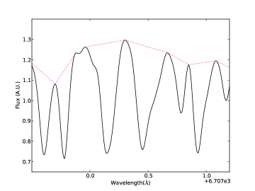
Figure 1: Small region of the Gl 205 spectra illustrating pseudo equivalent width line measurement. The red dotted line represents the ‘peak-to-peak’ flux.

The next step consisted in the investigation of the correlation between the measured EWs and the reference values for [Fe/H] and $T_{eff}$. Fig. 2 shows the histograms of the partial correlation coefficient values of the EWs with the value of the metallicity and effective temperature (solid blue and dashed green lines respectively). The partial correlation coefficient is defined as the correlation coefficient of one parameter keeping the other fixed. We observe, in Fig. 2 that a significant amount of lines have good correlation values with the parameters.

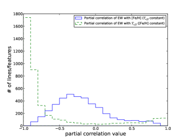
Figure 2: Histograms of the partial correlations of [Fe/H] (solid blue histogram) and $T_{eff}$ (dashed green histogram).

Then we did a least squares linear fit of the EWs with the metallicity and effective temperature. The reference values were calculated with the calibration of Neves et al. (2012), for [Fe/H], and with the three ($V-J$, $V-H$, and $V-K_{S}$) photometric calibrations of Casagrande et al. (2008), for $T_{eff}$, where we took the average value. From each line/feature $i$ of every star $m$ we calculate a EW value. Then we have

$$W_{i,m}=\alpha_{i}[Fe/H]_{m}^{T}+\beta_{i}T_{eff,m}^{T}+\gamma_{i},$$ (2)

where $W$ is the matrix containing the EWs, and both $[Fe/H]^{T}$, and $T_{eff}^{T}$ are the transpose vectors of the parameter values. The $\alpha$ and the $\beta$ are the coefficients related to metallicity and effective temperature, respectively, while $\gamma$ is an independent coefficient. The error associated to each parameter $p$ is calculated as

$$\epsilon_{p}=\sqrt{RSS.J},$$ (3)

where RSS is the residual sum of squares, expressed as

$$RSS=\frac{\sum{(x_{i,model}-x_{i})^{2}}}{n_{obs}-n_{coef}},$$ (4)

and $J$ is the diagonal of the estimate of the jacobian matrix around the solution. The $x_{i,model}$, $x_{i}$, $n_{obs}$, and $n_{coef}$ from Eq. 3 are, respectively, the predicted value of the data, $x_{i}$, by the regression model, the data values, the number of data points, and the number of coefficients. We assume that both metallicity and effective temperature are independent and do not correlate with each other. This assumption was tested by perturbing each parameter in turn by introducing an positive or negative offset and then calculating both parameters. There was no difference in the obtained values of the unperturbed parameter. We also tried to use the full covariance matrix to calculate the uncertainties but in the end we got a worse result for the dispersion. Therefore, we decided to use only the diagonal values of the covariance matrix. The total error of the coefficients associated to each line $i$ can then be written as

$$\epsilon_{i}=\sqrt{\epsilon_{\alpha}^{2}+\epsilon_{\beta}^{2}+\epsilon_{\gamma}^{2}}.$$ (5)

The aim of our technique is to increase the precision of both [Fe/H] and $T_{eff}$ determinations. To do that we need to obtain the values of the metallicity and effective temperature via a weighted least squares refit, that is obtained after a left multiplication of $(C^{T}C)^{-1}C^{T}$ on both terms of Eq. 2, where $C$ is the calibration matrix or the coefficient matrix, that can be written as

$$C=\left[\begin{array}[]{ccc}\alpha_{1,1}&\beta_{1,2}&\gamma_{1,3}\\ \alpha_{2,1}&\beta_{2,2}&\gamma_{2,3}\\ ...&...&...\\ \alpha_{I,1}&\beta_{I,2}&\gamma_{I,3}\end{array}\right],$$ (6)

and $C^{T}$ is the transpose of $C$. The refit is then expressed, for each star $m$, as

$$\left[\begin{array}[]{c}[Fe/H]\\ T_{eff}\\ \Gamma\end{array}\right]=(C^{T}C)^{-1}C^{T}W,$$ (7)

where $\Gamma$ is the parameter related to the independent $\gamma$ coefficients.

In order to correct the offset of our method we added an extra parameter, while adding a corresponding dimension in Eq. 6, that corresponds to an array of ones. The updated matrix $C$ has now dimension $I\times 4$ instead of $I\times 3$, where $I$ has the value of the number of lines.

Finally we introduce a weight to Eq. 7, using a Levenberg-Marquardt (Press et al. 1992) algorithm. We can write the elements of the normalised weight $E$ as

$$E_{i}=\frac{1/\epsilon_{i}^{2}}{\sum{1/\epsilon_{i}^{2}}}.$$ (8)

Other methods were tested, such as choosing lines/features with the best correlations or partial correlations with the parameters. However, the weighted least squares approach performed best at minimising the uncertainties of both metallicity and temperature.

2.2 A posteriori sample selection

At this stage we observed that some stars appeared as outliers in the plots of the pseudo EWs versus the reference [Fe/H] and $T_{eff}$ for many lines. We suspected that this behaviour was due to activity or rotation and did a a posteriori study of the impact of the activity with our technique. To this end, we used the normalized H$\alpha$ luminosity, $\log{L_{H_{\alpha}}/L_{bol}}$, from Reiners et al. (2012), for the stars in common with our full sample, as well as the median of individual measurements of the $H_{\alpha}$ index defined by Gomes da Silva et al. (2011), kindly provided by the author. Table LABEL:table:full lists both activity indicators, in columns 5 and 6, for the stars in common with our sample. Fig. 3 depicts the relation between both indices, where we observe the inactive stars, in the bottom left corner of the diagram, a linear trend between the indices for increasingly active stars, and a very active star, Gl285, in the top right corner of diagram, where the $\log{L_{H_{\alpha}}/L_{bol}}$ indicator seems to have saturated. The dashed black lines show the limits above which the stars were excluded from the final sample, as described in the following paragraph.

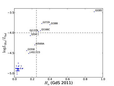
Figure 3: Normalized H$\alpha$ luminosity, taken from Reiners et al. (2012) versus the H_α index of Gomes da Silva et al. (2011) for the stars in common with our sample.The black dashed lines depict the limits that we have established for the sample selection.

Fig. 4 displays the normalized H$\alpha$ luminosity and the $H_{\alpha}$ index defined by Gomes da Silva et al. (2011) as a function of the difference between the parameters obtained with our method and the initial parameters. The legend in panels c) and d) depict the stellar spectra with S/N $\geq$ 100 (blue dots), S/N between 30 and 100 (black crosses), S/N between 30 and 25 (red circles), and S/N lower than 25 (green stars). We observe no clear correlation of the activity indices or S/N with [Fe/H]. Regarding $T_{eff}$ however, we can see that there is a clear trend towards lower temperatures with both activity indices. To take this trend into account we decided to perform an activity cut, excluding all stars with $\log{L_{H_{\alpha}}/L_{bol}}\geq-4.0$ and H$\alpha\geq 0.25$ from our final sample. We also note a trend of H$\alpha$ with $T_{eff}$ towards higher temperatures for stars with S/N $<$ 25 (see bottom right corner of Fig. 4 d). The trends of our method with S/N are studied in detail in Sect. 2.4.

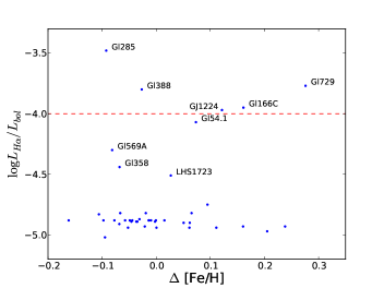
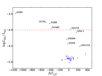
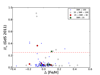
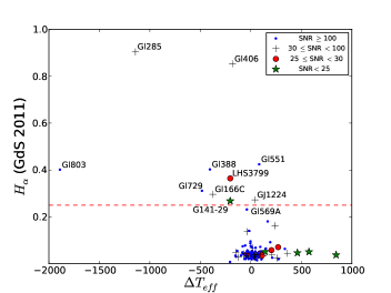
Figure 4: a) Normalized H$\alpha$ luminosity taken from Reiners et al. (2012) as a function of $\Delta$[Fe/H]; b) Normalized H$\alpha$ luminosity taken from Reiners et al. (2012) as a function of $\Delta T_{eff}$; c) H${\alpha}$ index defined by Gomes da Silva et al. (2011) versus $\Delta$[Fe/H]; d) H${\alpha}$ index defined by Gomes da Silva et al. (2011) versus $\Delta T_{eff}$. The stars in common were taken from our full sample. The red dashed lines mark the limits above which the stars were excluded from the final sample.

In the end, with a final sample of 65 stars, we obtain a dispersion of 0.08 dex for the metallicity and 91K for the effective temperature, as shown in Fig. 5. The technique is valid between -0.85 to 0.26 dex for [Fe/H], 2800 to 4100 K for $T_{eff}$, and between M0.0 to M5.0. The dispersion around the calibration is quantified by the root mean square error (RMSE), and defined as

$$RMSE=\sqrt{\frac{\sum{(x_{i}-x_{ref})^{2}}}{n_{obs}-n_{coef}}},$$ (9)

where $x_{i}$ is the estimated quantity, $x_{ref}$ the reference value for the same quantity, $n_{obs}$ the number of calibrators and $n_{coef}$ the number of parameters used in the method (four in this case).

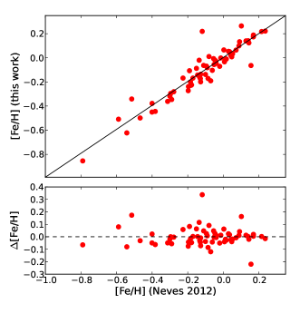
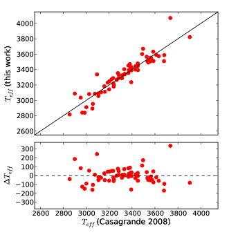
Figure 5: (a) [Fe/H] comparison between this work and the photometric calibration of Neves et al. (2012); (b) $T_{eff}$ comparison between this work and the photometric calibration of Casagrande et al. (2008).

The calculated parameters as well as the reference determinations for [Fe/H] and $T_{eff}$ are listed in Table 2. Columns 1 and 3 contain the values for the reference calibrations, while columns 2 and 4 show the values obtained with our technique. We emphasise here that we only get an improvement on the precision. The accuracy of the method as well as its systematics are tied to the original determinations of the parameters.

Table 2: Our sample table with the reference and calibrated metallicity and effective temperature. Sorted by right ascension.

star	[Fe/H]N12	[Fe/H]NEW	$T_{effC08}$	$T_{effNEW}$
	[dex]	[dex]	[K]	[K]
Gl1	-0.40	-0.45	3528	3567
Gl54.1	-0.40	-0.38	2901	3088
Gl87	-0.30	-0.32	3565	3555
Gl105B	-0.14	-0.02	3054	2894
HIP12961	-0.12	0.22	3904	3823
LP771-95A	-0.51	-0.34	3393	3236
GJ163	0.00	0.07	3223	3276
Gl176	0.02	-0.01	3369	3355
GJ179	0.14	0.12	3076	3086
Gl191	-0.79	-0.85	3679	3510
Gl205	0.17	0.19	3497	3670
Gl213	-0.19	-0.11	3026	3082
Gl229	-0.04	-0.03	3586	3633
HIP31293	-0.04	-0.05	3312	3288
HIP31292	-0.11	-0.06	3158	3184
Gl250B	-0.09	-0.08	3369	3453
Gl273	-0.05	-0.01	3107	3090
Gl300	0.09	0.13	2965	2841
GJ2066	-0.09	-0.17	3388	3421
GJ317	0.22	0.22	3130	3106
Gl341	-0.14	-0.14	3633	3575
GJ1125	-0.15	-0.09	3162	3112
Gl357	-0.30	-0.30	3335	3344
Gl358	0.01	-0.01	3240	3178
Gl367	-0.09	-0.07	3452	3394
Gl382	0.04	0.02	3429	3401
Gl393	-0.13	-0.20	3396	3431
GJ3634	-0.02	-0.07	3332	3405
Gl413.1	-0.06	-0.10	3373	3394
Gl433	-0.13	-0.17	3450	3480
Gl436	0.01	-0.03	3277	3354
Gl438	-0.31	-0.36	3536	3505
Gl447	-0.23	-0.17	2952	3036
Gl465	-0.54	-0.62	3382	3472
Gl479	0.05	0.01	3238	3218
Gl514	-0.13	-0.16	3574	3526
Gl526	-0.18	-0.22	3545	3515
Gl536	-0.13	-0.14	3546	3525
Gl555	0.13	0.14	2987	2839
Gl569A	0.16	-0.06	3235	3289
Gl581	-0.18	-0.20	3203	3248
Gl588	0.07	0.06	3284	3291
Gl618A	-0.05	-0.06	3242	3200
Gl628	-0.05	-0.02	3107	3057
GJ1214	0.03	0.05	2856	2817
Gl667C	-0.47	-0.50	3431	3445
Gl674	-0.18	-0.23	3284	3334
GJ676A	0.10	0.26	3734	4071
Gl678.1A	-0.10	-0.14	3611	3591
Gl680	-0.07	-0.19	3395	3390
Gl682	0.09	0.10	3002	2912
Gl686	-0.29	-0.35	3542	3493
Gl693	-0.28	-0.28	3188	3232
Gl699	-0.59	-0.51	3094	3338
Gl701	-0.20	-0.27	3535	3510
Gl752A	0.04	0.05	3336	3339
Gl832	-0.17	-0.17	3450	3446
Gl846	-0.08	0.01	3682	3588
Gl849	0.24	0.22	3200	3143
Gl876	0.14	0.14	3059	2954
Gl877	-0.01	-0.00	3266	3266
Gl880	0.05	0.03	3488	3602
Gl887	-0.20	-0.24	3560	3507
Gl908	-0.38	-0.44	3587	3511
LTT9759	0.17	0.17	3316	3326

2.3 Estimation of the uncertainties

To validate our method and have a better understanding of the uncertainties of our measurements we performed a bootstrap resampling and calculated the root mean square error of validation (RMSE_V).

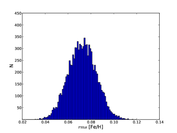
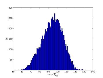
Figure 6: Histogram of the dispersion given by bootstrap for [Fe/H] (a) and $T_{eff}$ (b). The N is the number of trials.

The bootstrap method we implemented tests how the $rms$ of the method changes when using slightly different ‘bootstrapped’ samples. To have a statistical significative number we first created 10.000 virtual samples by randomly drawing with repetition, for each virtual sample, a number of stars equal to the size of our sample. The random drawing followed a random uniform distribution. Then we calculated the $rms$ for each trial and measured the $1\sigma$ gaussian equivalent interval between 15.9% and 84.1% from the resulting distribution, following the procedure of e.g. Burgasser et al. (2003); Neves et al. (2013). The distributions of the $rms$ for both parameters are depicted in Fig. 6. The final result shows a variation of the $rms$ of the [Fe/H] and $T_{eff}$ by $\pm 0.01$ dex and $\pm 13$ K respectively.

The calculation of the RMSE_V is a predicted residual sum of squares (PRESS) procedure (Weisberg 2005) and follows the description in the Appendix of Rojas-Ayala et al. (2012). In short, we try to obtain the original value of the metallicity and temperature of each star $i$ of the technique leaving that star out when calculating the parameters. Then, we calculate the residuals, or the difference between the original and obtained value for each star and add them up in quadrature. The PRESS statistic is then defined as

$$PRESS=\sum{(y_{i}-y_{ref}})^{2},$$ (10)

where $y_{i}$ is the estimated value of the parameter and $y_{ref}$ is the reference value of the measured quantity. From here we can calculate the root mean squared error of validation,

$$RMSE_{V}=\sqrt{\frac{PRESS}{n_{V}}},$$ (11)

where $n_{V}$ is the number of calibrators. The RMSE_V value can then be used to obtain confidence intervals. We obtain a RMSE_V value of 0.12 dex and $\sim$ 293 K for the [Fe/H] and $T_{eff}$ respectively and will use these values as $1\sigma$ confidence intervals, assuming a normal cumulative distribution function. Table 3 summarises our results.

Table 3: Uncertainty estimators for [Fe/H] and $T_{eff}$.

Estimator	[Fe/H]	$T_{eff}$
	[dex]	[K]
RMSE	0.08	91
Bootstrap	0.08$\pm$0.01	91$\pm$13
RMSEV	0.12	293

We observe that the uncertainties calculated with the different techniques are consistent with each other. The uncertainty for $T_{eff}$ is large but is in line with the expected uncertainties. We also perturbed our sample by introducing an offset in [Fe/H] or $T_{eff}$, as explained in Sect. 2.1 but found that it does not affect the measurement of the parameters. In the end we assume our final uncertainty to be the maximum uncertainty of the RMSE given by the bootstrap, that translates into 0.09 dex for [Fe/H] and 110 K for $T_{eff}$.

2.4 Testing our technique as a function of resolution and S/N

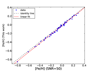
Figure 7: [Fe/H] of our procedure versus the [Fe/H] obtained with S/N=50.The identity line is depicted in dashed black. The solid red line shows the linear fit.

To further test our method, we calculated the dispersion of the parameters as a function of the resolution and S/N. The first step consisted in the study of the behaviour of the procedure as a function of S/N only. We injected random Gaussian noise in the spectra of the sample to obtain spectra with S/N @ 5500 Å  between 100 and 10. Then, we calculated linear fits between the [Fe/H] and $T_{eff}$ obtained with the lower S/N spectra and the values of our method, for the full S/N range, as shown in Fig. 7 for [Fe/H] and S/N=50. The dashed black line marks the identity line while the red line represents a linear fit to the data.

Fig. 8 depicts the slope and offset of the linear fits for [Fe/H] and $T_{eff}$, as a function of S/N. We observe a deviation from the identity line as the S/N decreases as expected, except in d), where the offset of $T_{eff}$ is reasonably constant, on average, with S/N. From here we investigated the cause of this trend and found that the measured EWs, roughly quantified as the median of all EWs, follow similar trends with S/N, as shown in Fig. 9 the for the star Gl479 ([Fe/H] = 0.01 dex, $T_{eff}$ = 3218 K) as example. The observed trends are similar in other stars, with different metallicities and effective temperatures.

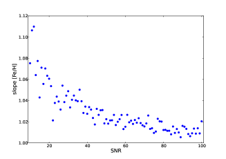
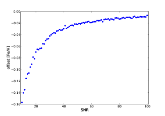
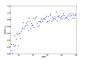
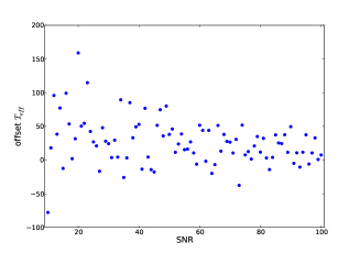
Figure 8: Slope and offset of [Fe/H] and $T_{eff}$ of our work as a function of S/N for star Gl479.

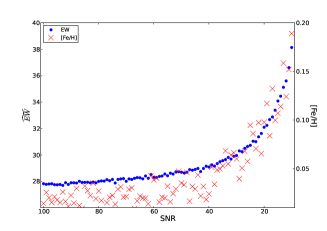
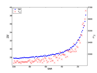
Figure 9: Median of the pseudo EWs and [Fe/H] (a) or $T_{eff}$ (b) as a function of S/N for star Gl479.

Using this information, we corrected the values of both parameters for all stars of our sample with S/N $<$ 100, where [Fe/H] (Corrected) = $a$[Fe/H] (Degraded) + $b$, and $T_{eff}$ (Corrected) = $aT_{eff}$ (Degraded) + $b$. The $a$ is the slope and $b$ is the offset. The uncertainties associated with each correction were estimated by calculating the dispersion of the residuals. However, we observed that these uncertainties are very small compared to the the final uncertainty of our method, as shown in Sect. 2.3. Therefore, we assumed the uncertainty of our method for all stars, except for the active ones, according to the two estimated activity thresholds calculated in Sect. 2.2. In this case, we used the initial values of the parameters, calculated with the calibrations of Neves et al. (2012) and Casagrande et al. (2008). At this point, we also decided not to use our new values for stars with S/N $\leq$ 25, because the correction was not good enough to obtain a reasonable value for the objects depicted as green stars in Fig. 4. Moreover, we note that the stars LHS 1513 and Gl 803 give an estimated [Fe/H] value of $-1.51$ and $0.46$ dex respectively, calculated with the calibration of Neves et al. (2012), our reference scale. Both values are outside the range of this method and will not be used. Table LABEL:table:full shows the corrected results, along with the previous values of [Fe/H] from Neves et al. (2013). Column 1 describes the star designation and column 2 and 3, the right ascension and declination of the star, respectively. Column 4 depicts the S/N, column 5 the normalized $H\alpha$ index taken from Reiners et al. (2012), and column 6 the $H\alpha$ index described by Gomes da Silva et al. (2011). Column 7 shows the metallicity calculated with the coefficient matrix used in our previous work, Neves et al. (2013), column 8 the [Fe/H] obtained in our work, along with its associated error in column 9. The $T_{eff}$ values of our stars, and its uncertainties are described in columns 10 and 11.

In the second step of this test we modified both resolution and S/N of our sample spectra. The resolution of the HARPS spectra was degraded by convolving the spectra with a normalised Gaussian curve, simulating the instrumental profile, with $FWHM=\lambda/R$, where $\lambda$ is the wavelength and $R$ the resolution we intend to obtain. From here, the standard deviation of the Gaussian is calculated with the well known formula

$$\sigma=\frac{FWHM}{2\sqrt{2\log{2}}}.$$ (12)

The $\sigma$ was adjusted to the HARPS resolution ($R\sim 115.000$) and to the original S/N @ $5500\AA$ of each spectrum. The final value for $\sigma$ is then

$$\sigma^{\prime}=\sqrt{\sigma^{2}-\sigma_{HARPS}^{2}}.$$ (13)

Figures 10 and 11 show the difference of our parameters against the degraded values, as a function of resolution (while the S/N is kept constant at 100) and as a function of S/N (while the resolution is kept constant at 100.000) for [Fe/H] and $T_{eff}$ respectively. The red dotted line depicts the offset of the residuals.

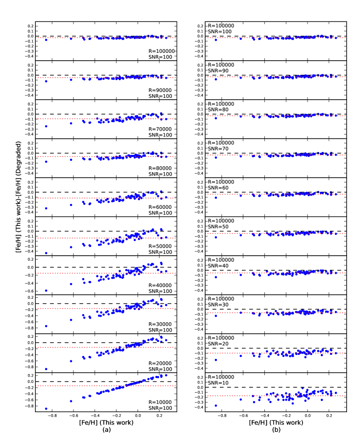
Figure 10: Difference of the [Fe/H] for this work and the [Fe/H] calculated with different resolution/signal-to-noise combinations as a function of the resolution and S/N.

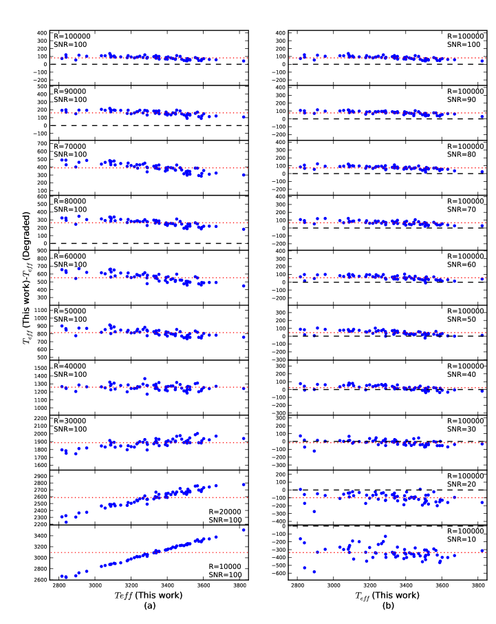
Figure 11: Difference of the $T_{eff}$ for this work and the $T_{eff}$ calculated with different resolution/signal-to-noise combinations as a function of the resolution and S/N.

From the two Figures we observe the existence of linear trends for different resolutions and S/N. To correct these trends we performed a linear fit for each Resolution/signal-to-noise combination with the functional form [Fe/H] (This work)$=a$[Fe/H] (Degraded) + $b$ for metallicity, and $T_{eff}$ (This work)$=aT_{eff}$ (Degraded) + $b$ for effective temperature. The values for each combination are shown in Table 5.

Table 5: Linear fit coefficients $a$ and $b$ from the relation between the values of our parameters and the values calculated for different combinations of resolution and S/N.

S/N	100		90		80		70		60
Resolution	a	b	a	b	a	b	a	b	a	b
100000	1.0573	-0.0257	1.0645	-0.0269	1.0572	-0.0275	1.0721	-0.0304	1.0686	-0.0353
95000	1.0793	-0.0304	1.0786	-0.0343	1.0849	-0.0358	1.0766	-0.0401	1.0740	-0.0455
90000	1.0947	-0.0428	1.1111	-0.0430	1.0973	-0.0472	1.1024	-0.0488	1.1029	-0.0521
85000	1.1164	-0.0529	1.1345	-0.0511	1.1313	-0.0557	1.1451	-0.0592	1.1209	-0.0639
80000	1.1522	-0.0630	1.1527	-0.0652	1.1545	-0.0670	1.1595	-0.0694	1.1587	-0.0749
75000	1.1819	-0.0751	1.1859	-0.0790	1.1774	-0.0801	1.1891	-0.0838	1.1967	-0.0877
70000	1.2184	-0.0877	1.2271	-0.0905	1.2309	-0.0920	1.2354	-0.0939	1.2441	-0.1018
65000	1.2614	-0.0997	1.2781	-0.1045	1.2739	-0.1075	1.2850	-0.1094	1.2849	-0.1149
60000	1.3350	-0.1191	1.3306	-0.1174	1.3361	-0.1206	1.3408	-0.1255	1.3437	-0.1305
55000	1.3949	-0.1372	1.4058	-0.1370	1.4039	-0.1417	1.3962	-0.1439	1.4440	-0.1518
50000	1.4859	-0.1499	1.5020	-0.1559	1.5317	-0.1590	1.5211	-0.1631	1.5289	-0.1666
45000	1.5768	-0.1623	1.5924	-0.1670	1.5550	-0.1700	1.5998	-0.1726	1.5686	-0.1811
40000	1.6667	-0.1739	1.6608	-0.1837	1.6628	-0.1912	1.6434	-0.1903	1.6910	-0.1976
35000	1.6830	-0.1907	1.7071	-0.1930	1.7183	-0.1984	1.6553	-0.2061	1.6662	-0.2076
30000	1.7031	-0.1998	1.6868	-0.2016	1.6715	-0.2080	1.6561	-0.2102	1.6526	-0.2109
25000	1.7480	-0.2035	1.7205	-0.2016	1.7607	-0.2103	1.7139	-0.2077	1.7232	-0.2126
20000	1.8697	-0.1965	1.8721	-0.1996	1.9415	-0.2054	1.7788	-0.1984	1.7328	-0.1986
15000	2.2339	-0.1950	2.1304	-0.1933	2.3825	-0.2044	2.4904	-0.2125	2.3611	-0.2164
10000	3.6228	-0.2062	2.6636	-0.1899	2.8711	-0.1999	2.6645	-0.2022	0.1404	-0.1154
S/N	50		40		30		20		10
Resolution	a	b	a	b	a	b	a	b	a	b
100000	1.0749	-0.0400	1.0863	-0.0496	1.0652	-0.0669	1.0962	-0.0962	1.1196	-0.1781
95000	1.1026	-0.0480	1.0960	-0.0566	1.0912	-0.0775	1.1092	-0.1012	1.0946	-0.1912
90000	1.1050	-0.0574	1.1229	-0.0683	1.1226	-0.0842	1.1506	-0.1184	1.1492	-0.2043
85000	1.1322	-0.0698	1.1658	-0.0794	1.1645	-0.0921	1.1767	-0.1251	1.1727	-0.2200
80000	1.1730	-0.0826	1.1852	-0.0877	1.2021	-0.1082	1.2164	-0.1443	1.1864	-0.2345
75000	1.2013	-0.0947	1.2168	-0.1039	1.2283	-0.1229	1.2608	-0.1553	1.1913	-0.2321
70000	1.2298	-0.1103	1.2395	-0.1177	1.2697	-0.1359	1.2593	-0.1605	1.2609	-0.2620
65000	1.3065	-0.1210	1.3072	-0.1315	1.3125	-0.1482	1.3743	-0.1880	1.2488	-0.2867
60000	1.3658	-0.1417	1.3886	-0.1524	1.3698	-0.1694	1.3925	-0.1991	1.2093	-0.2847
55000	1.4498	-0.1584	1.4282	-0.1685	1.4266	-0.1878	1.4316	-0.2206	1.4105	-0.3137
50000	1.5178	-0.1755	1.5140	-0.1952	1.5464	-0.2043	1.5296	-0.2523	1.2569	-0.3076
45000	1.6032	-0.1942	1.5460	-0.2028	1.6107	-0.2200	1.5216	-0.2526	1.2952	-0.3159
40000	1.6677	-0.2050	1.5879	-0.2159	1.5324	-0.2321	1.4905	-0.2579	1.2183	-0.3194
35000	1.6524	-0.2123	1.6276	-0.2232	1.6483	-0.2486	1.4189	-0.2579	1.0835	-0.2904
30000	1.7535	-0.2277	1.6359	-0.2315	1.5524	-0.2371	1.4348	-0.2617	1.0072	-0.2814
25000	1.7370	-0.2223	1.5786	-0.2180	1.6060	-0.2398	1.5160	-0.2570	0.9624	-0.2582
20000	1.7250	-0.2059	1.8548	-0.2279	1.6821	-0.2321	1.1003	-0.2154	0.8352	-0.2465
15000	1.6573	-0.1903	1.7403	-0.2065	1.9868	-0.2428	1.0153	-0.2100	0.3012	-0.1615
10000	1.5151	-0.1772	1.3777	-0.1797	0.8703	-0.1678	1.2768	-0.2351	0.5612	-0.2087

(a) [Fe/H]

S/N	100		90		80		70		60
Resolution	a	b	a	b	a	b	a	b	a	b
100000	0.9391	279	0.9395	273	0.9394	271	0.9306	293	0.9294	288
95000	0.9305	342	0.9156	387	0.9182	377	0.9098	396	0.9164	364
90000	0.9137	435	0.8986	482	0.9167	416	0.9087	435	0.9028	447
85000	0.8802	582	0.8873	558	0.8811	575	0.8729	590	0.8879	538
80000	0.8726	654	0.8705	658	0.8646	672	0.8676	655	0.8524	694
75000	0.8524	767	0.8502	769	0.8497	767	0.8444	778	0.8511	750
70000	0.8339	880	0.8360	872	0.8478	829	0.8305	876	0.8418	830
65000	0.8286	957	0.8290	952	0.8277	953	0.8396	912	0.8354	917
60000	0.8298	1025	0.8240	1039	0.8457	977	0.8389	989	0.8576	932
55000	0.8553	1050	0.8583	1040	0.8743	994	0.8712	997	0.8711	993
50000	0.8864	1101	0.8870	1096	0.8892	1088	0.8896	1083	0.9061	1036
45000	0.9083	1227	0.9243	1184	0.9139	1204	0.9318	1159	0.9243	1169
40000	0.9733	1313	0.9820	1294	0.9832	1284	0.9873	1274	1.0037	1227
35000	1.0585	1451	1.0587	1445	1.0673	1424	1.0664	1414	1.0656	1408
30000	1.2080	1587	1.2091	1573	1.2198	1554	1.2030	1565	1.2386	1498
25000	1.4745	1717	1.4831	1699	1.4847	1683	1.5107	1641	1.5034	1624
20000	1.9977	1842	2.0116	1817	1.9598	1834	1.9840	1793	1.9362	1792
15000	3.1029	1946	3.1103	1914	2.9692	1936	3.0119	1867	3.0566	1775
10000	6.8985	1681	6.2175	1775	6.2539	1685	6.2833	1548	5.6847	1562
S/N	50		40		30		20		10
Resolution	a	b	a	b	a	b	a	b	a	b
100000	0.9249	291	0.9223	281	0.9363	198	0.9001	245	0.8592	179
95000	0.9148	358	0.9194	327	0.9000	352	0.8961	290	0.8793	130
90000	0.9083	419	0.8891	459	0.8993	390	0.8898	353	0.8804	161
85000	0.8733	572	0.8741	547	0.8894	462	0.8595	492	0.8308	361
80000	0.8665	640	0.8566	647	0.8626	597	0.8649	512	0.8964	178
75000	0.8492	742	0.8506	714	0.8534	674	0.8623	571	0.8284	465
70000	0.8494	796	0.8407	806	0.8479	750	0.8816	572	0.8621	402
65000	0.8438	878	0.8257	915	0.8466	816	0.8567	713	0.8433	519
60000	0.8477	948	0.8705	863	0.8817	797	0.8801	725	0.9280	332
55000	0.8968	912	0.8730	954	0.8778	913	0.8882	817	0.8757	608
50000	0.9027	1032	0.9235	962	0.9400	889	0.9670	730	0.9068	629
45000	0.9462	1109	0.9496	1078	0.9855	956	1.0141	791	1.0176	467
40000	1.0046	1211	1.0191	1157	1.0381	1074	1.0690	901	0.9749	794
35000	1.1054	1317	1.1249	1252	1.1198	1204	1.1365	1059	1.0122	939
30000	1.2608	1441	1.2615	1401	1.2422	1353	1.2352	1216	1.2106	780
25000	1.5634	1525	1.5462	1491	1.4461	1513	1.4680	1287	1.1921	1163
20000	2.0226	1665	2.0712	1542	1.9740	1475	1.8071	1364	1.3502	1271
15000	3.0308	1698	2.8844	1623	2.7979	1454	2.3031	1400	1.4130	1486
10000	4.8757	1643	4.4861	1557	3.1564	1817	1.9481	2046	0.3888	2893

(b) $T_{eff}$

From here we calculated the dispersion of the difference between the corrected parameter values and the ones obtained from our original determinations, and added this dispersion with the one from our method in quadrature. Table 6 shows the results. The horizontal header of both tables correspond to the S/N of the spectra, between 100 and 10, while the vertical header depicts their resolution, from 100.000 to 10.000. The row with the resolution number is the value of the dispersion of our technique using the corresponding resolution/signal-to-noise combination. This table should be used as a guideline for the uncertainties of the parameters when using spectra other than HARPS.

Table 6: Dispersion of the residuals of the parameters as a function of the resolution and S/N.

S/N	100	90	80	70	60	50	40	30	20	10
Resolution
100000	0.081	0.081	0.081	0.081	0.082	0.082	0.083	0.083	0.089	0.105
95000	0.082	0.082	0.082	0.082	0.082	0.083	0.083	0.086	0.091	0.107
90000	0.082	0.082	0.082	0.082	0.083	0.083	0.084	0.087	0.089	0.103
85000	0.083	0.083	0.083	0.083	0.085	0.085	0.085	0.085	0.094	0.116
80000	0.084	0.084	0.084	0.085	0.085	0.085	0.087	0.089	0.095	0.113
75000	0.085	0.085	0.086	0.086	0.086	0.087	0.089	0.092	0.097	0.123
70000	0.088	0.087	0.088	0.088	0.088	0.091	0.091	0.094	0.100	0.122
65000	0.090	0.090	0.091	0.092	0.094	0.095	0.096	0.100	0.107	0.125
60000	0.092	0.096	0.093	0.095	0.097	0.099	0.098	0.102	0.109	0.144
55000	0.098	0.099	0.101	0.102	0.102	0.101	0.109	0.113	0.126	0.144
50000	0.108	0.109	0.109	0.113	0.115	0.118	0.120	0.124	0.132	0.161
45000	0.125	0.126	0.129	0.128	0.135	0.131	0.138	0.138	0.148	0.174
40000	0.146	0.147	0.148	0.151	0.149	0.152	0.156	0.161	0.174	0.185
35000	0.168	0.169	0.170	0.172	0.174	0.175	0.174	0.176	0.187	0.203
30000	0.189	0.189	0.190	0.191	0.192	0.189	0.194	0.199	0.202	0.212
25000	0.205	0.207	0.205	0.208	0.207	0.207	0.211	0.212	0.209	0.219
20000	0.220	0.217	0.218	0.220	0.219	0.221	0.219	0.219	0.228	0.225
15000	0.227	0.228	0.226	0.224	0.226	0.231	0.229	0.227	0.231	0.235
10000	0.231	0.233	0.233	0.233	0.236	0.234	0.234	0.235	0.231	0.233

(a) [Fe/H]

S/N	100	90	80	70	60	50	40	30	20	10
Resolution
100000	92	92	92	92	93	93	94	96	103	118
95000	92	92	92	93	93	93	95	97	103	116
90000	93	93	94	93	94	95	95	98	99	116
85000	93	94	93	94	94	94	95	95	102	115
80000	94	94	94	95	94	95	96	99	102	117
75000	93	94	94	95	94	96	96	97	101	120
70000	94	95	95	95	95	96	97	99	103	116
65000	95	95	94	95	95	96	97	97	102	117
60000	95	95	96	96	95	97	97	100	102	115
55000	95	95	96	95	95	97	98	101	107	127
50000	95	95	96	96	96	98	99	103	104	123
45000	97	96	97	97	97	96	99	101	108	129
40000	98	98	97	99	99	99	100	106	113	128
35000	99	100	100	99	99	100	103	106	114	148
30000	101	101	103	102	103	101	106	111	123	147
25000	104	104	108	105	106	108	113	115	129	161
20000	112	110	111	118	115	116	116	125	143	179
15000	116	120	126	125	130	129	146	154	179	216
10000	135	133	155	146	167	177	185	214	235	259

(b) $T_{eff}$

From Table 6 and Figs. 10 and 11 we observe that, as the resolution degrades, the dispersion and offset of the residuals increase. In the case of [Fe/H], the dispersion value holds well for a resolution higher and equal to 40.000 respectively. From 35.000 and lower resolutions we observe that the uncertainties of the residuals are similar or greater than the original dispersion (0.17 dex), meaning that the method is not useful any more, providing we have precise parallaxes and visual magnitudes. Regarding $T_{eff}$, we consider that the method is valid for the same resolution and S/N intervals as in [Fe/H]. We also limit the use of the technique for spectra with S/N greater than 25, as we cannot properly correct the parameters, as we have previously seen in this Section. From here we investigated the nature of these correlations by plotting the median of all EWs with the parameters, as a function of resolution (with S/N=100), for a metal-poor star Gl191 ([Fe/H] = -0.85 dex, $T_{eff}$ = 3510 K) and a metal-rich star, GJ 317 ([Fe/H] = 0.22 dex, $T_{eff}$ = 3106 K), as it was previously done for S/N, and shown in Fig. 9. Fig. 12 pictures the results. The blue dots depict the median of the pseudo EWs while the red crosses show the metallicity or the effective temperature.

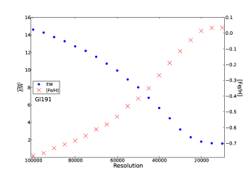
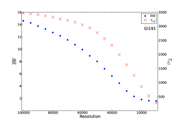
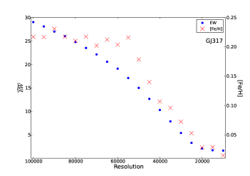
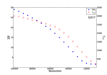
Figure 12: Measured median of the pseudo EWs, [Fe/H] and $T_{eff}$ as a function of resolution for the stars Gl191 (a and b) and GJ317 (c and d). The blue dots depict the median of the pseudo EWs while the red crosses show the metallicity or the effective temperature.

We observe that the EW and the parameters follow similar trends as the resolution degrades, as expected, except in Fig. 12 a) where metallicity has an opposite trend to the EW. We do not know the cause of the different trend.

The increasing dispersions and offsets with the resolution observed in Fig. 10 and 11 should originate from the nature of our ‘peak-to-peak’ technique because it does not consider the continuum. As the resolution gets worse, more and more flux from the ‘peak-to-peak’ region is lost to the line wings. However, as the resolution decreases there is an increase of line blending that makes the measurement of the correct flux of the each line/feature increasingly difficult. Moreover, we also observe from Fig. 2 that we have similar numbers of correlation and anti-correlations of the lines with [Fe/H], and the overall effect of the weighted lines may change as the resolution degrades. The mix of any of these effects may be the reason behind we get different trends for [Fe/H] from Gl191 (Fig. 12 a) and GJ436 (Fig. 12 c).

In order to validate our estimation of the uncertainties we used a sample of spectra of stars in common taken from the SOPHIE spectrograph (Bouchy & The Sophie Team 2006) archive. We downloaded individual observations taken with the ‘HR’ ($R\sim 75.000$) and ‘HE’ ($R\sim 40.000$) modes, with the reference fiber exposed to the sky rather than to the Thorium-Argon calibration lamp, to avoid potential contamination. The ‘HR’ sample is comprised of 12 stars in common while the ‘HE’ sample contains only 5 stars.

First, we summed the individual spectra of each star, after correcting the radial velocity of each spectrum, and calculated their pseudo EWs. The S/N of the summed spectra for each star in common range from 34 to more than 600. Then, we calculated the metallicity and effective temperature and applied the appropriate corrections shown in Table 5, following the resolution and S/N of each spectra. The final values of the parameters are displayed in Table 7. Column 2 lists the resolution, column 3 the S/N, and column 4 to 7 the parameters of our method and the ones obtained with the SOPHIE spectra, respectively.

Table 7: [Fe/H] and $T_{eff}$ calculated from a sample in common with SOPHIE observations.

Star	Resolution	S/N	[Fe/H] (This work)	[Fe/H] (SOPHIE)	$T_{eff}$ (this work)	$T_{eff}$ (SOPHIE)
			[dex]	[dex]	[K]	[K]
Gl699	75.000	102	-0.51	-0.39	3338	3292
Gl686	75.000	557	-0.35	-0.28	3493	3529
Gl87	75.000	147	-0.32	-0.21	3555	3472
GJ1125	75.000	64	-0.09	0.07	3112	3049
Gl273	75.000	62	-0.01	-0.02	3090	3057
GJ2066	75.000	86	-0.17	-0.07	3421	3249
Gl393	75.000	91	-0.20	-0.10	3431	3326
Gl514	75.000	636	-0.16	-0.11	3526	3501
Gl846	75.000	175	0.01	0.04	3588	3551
Gl176	75.000	79	-0.01	0.06	3355	3196
GJ179	75.000	34	0.12	0.06	3086	2878
Gl436	75.000	150	-0.03	0.04	3354	3304
Gl447	40.000	56	-0.17	-0.15	3036	3202
Gl213	40.000	85	-0.11	-0.15	3082	3246
GJ1125	40.000	62	-0.09	-0.03	3112	3340
Gl846	40.000	79	0.01	0.27	3588	3762
GJ179	40.000	141	0.12	0.13	3086	3188

We obtain a $rms$ for the [Fe/H] of 0.088 and 0.123 dex for the ‘HR’ and the ‘HE’ samples respectively. Both dispersions are very close the expected dispersions for R=75.000 and R=40.000, as depicted in Table 6. For $T_{eff}$, we obtain a dispersion of 104 and 172 K for the ‘HR’ and ‘HE’ samples respectively. Both values are above the expected values, but in the case of the ’HR’ sample, the difference is only a few Kelvin. Regarding the ’HE’ sample, this difference is larger ($\sim$ 75 K), but the dispersion value is close to the one considered for the photometric calibration ($\sim$ 150 K). Moreover, we note that the sample size is very small (N=5). These results give us confidence and validate our uncertainty estimation method.

3 Comparison with the literature

A comparison with other studies in the literature was performed. This comparison allow us to evaluate the accuracy of our method and the possible systematics that it may suffer. Table LABEL:table:compfull shows our spectroscopic results compared to the ones found in the literature, for the stars in common. Column 1 depicts the star designations and column 2 informs if the star belongs or not to the selected sample that we used to calibrate our method. Columns 3 to 13 and columns 14 to 21 describe our [Fe/H] and $T_{eff}$ against the metallicity found in the literature, respectively. We note here that we only used the spectroscopic derived values for comparison. All active stars were excluded from this exercise.

We show in Table 9 the results of the comparison for the sample used in our technique and the full sample. The results for [Fe/H] are separated by photometric and spectroscopic techniques. The first column depicts the name of the method along with its reference. Column two and three describe the dispersion and offset. The last column reports the number of stars in common with our sample. We do not display the calibration of Mann et al. (2013a) in Table 9 because we only have two stars in common with them. However, we include the 4 measurements from the V- and K-band calibrations in the row ‘All [Fe/H] values’. We note here that we only compared stars in common for which we could calculate precise values of [Fe/H] and $T_{eff}$ with our methodology.

Table 9: Dispersion and offset of [Fe/H] and $T_{eff}$ from the residuals of the sample of the method and full sample against other studies. The last column shows the number of stars in common.

Photometric [Fe/H] calibrations	$rms$	offset	N
Bonfils et al. (2005)	0.11	-0.06	65
Schlaufman & Laughlin (2010)	0.11	0.02	65
Johnson et al. (2012)	0.19	0.05	65
Spectroscopic [Fe/H] determinations	$rms$	offset	N
All [Fe/H] values	0.11	0.05	55
Woolf & Wallerstein (2005)	0.09	-0.02	5
Rojas-Ayala et al. (2012)	0.12	0.03	19
Önehag et al. (2012)	0.08	0.05	8
Terrien et al. (2012)	0.07	0.06	7
Mann et al. (2013b)	0.16	0.11	7
Newton (2013)	0.11	0.07	5
$T_{eff}$ determinations	$rms$	offset	N
Woolf & Wallerstein (2005)	122	116	5
Rojas-Ayala et al. (2012)	299	246	19
Önehag et al. (2012)	160	64	8
Mann et al. (2013b)	167	133	7
Boyajian et al. (2012)	157	129	49
Rajpurohit et al. (2013a)	132	100	8

(a) Selected sample

Spectroscopic [Fe/H] determinations	$rms$	offset	N
Rojas-Ayala et al. (2012)	0.13	0.06	25
Newton (2013)	0.15	0.1	13
$T_{eff}$ values	$rms$	offset	N
Rojas-Ayala et al. (2012)	304	222	25
Boyajian et al. (2012)	149	111	55
Rajpurohit et al. (2013a)	181	133	12

(b) Full Sample

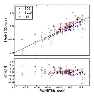
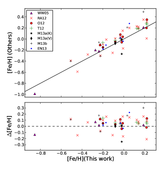
Figure 13: Upper panel: [Fe/H]-[Fe/H] plots comparing the values of this work, from the selected sample, against others in the literature. The solid black line of both (a) and (b) depict the identity line; Lower panel: Comparison plot residuals. The dashed black line marks the zero point of our technique. The plot (a) shows the results of our work versus three photometric calibrations taken from the literature, while plot (b) depicts the comparison between our results against other spectroscopic measurements.

The photometric [Fe/H] was calculated with the relations of Bonfils et al. (2005), Schlaufman & Laughlin (2010) and Johnson et al. (2012), while the spectroscopic [Fe/H] was taken directly from the works of Woolf & Wallerstein (2005), Rojas-Ayala et al. (2012), Önehag et al. (2012), Terrien et al. (2012), Newton (2013), and Mann et al. (2013b), except in the case of Mann et al. (2013a), where the values of the visible (their Eq. 8) and K-band (their Eq. 16) calibrations were provided directly by the author. We note that we used the average of the H- and K-band spectroscopic relations of Terrien et al. (2012). Also, we restricted the calculation of the photometric calibrations to the stars from the sample selection, for which we have precise photometries and parallaxes, to insure the best possible results in the comparison exercise.

Figure 13 portrays two [Fe/H]-[Fe/H] plots, with data taken from the selected sample. The left plot (a) shows the comparison of our sample with the works based on photometric scales. The blue dots, red crosses and black plus signs indicate the results of Bonfils et al. (2005), Schlaufman & Laughlin (2010), and Johnson et al. (2012) respectively. The right plot (b) depicts the comparison of our selected sample with other spectroscopic methods. The purple triangles, red crosses, red circles, green plus signs, black stars, black diamonds, black plus signs, and blue dots correspond to the measurements of Woolf & Wallerstein (2005), Rojas-Ayala et al. (2012), Önehag et al. (2012), Terrien et al. (2012), Mann et al. (2013a), Mann et al. (2013b), and Newton (2013) respectively. The (V) and (K) in Mann et al. (2013a) correspond to measurements performed with a V- and K-band calibration respectively. The solid black line in the upper panel of both plots defines an identity line. The lower panels show the residuals. The dashed black line marks the zero-point of the calibration.

For metallicity we observe a general agreement between our results and the ones from the literature. We note here that the calibration of Schlaufman & Laughlin (2010) is very similar to our reference calibration, from Neves et al. (2012), and this is the reason why we obtain a value of dispersion smaller than the one of the original calibration (0.11 vs 0.17 dex). The dispersion of the oldest photometric calibration (Bonfils et al. 2005) is surprisingly low (0.11 dex), considering that the original dispersion for this calibration is 0.20 dex. However, the Bonfils et al. (2005) is also similar to Schlaufman & Laughlin (2010) and Neves et al. (2012) which may explain part of the low dispersion. Regarding the Johnson et al. (2012) calibration, we obtain a $rms$ of 0.19 dex, higher that their reported value of 0.15 dex. The dispersion of the spectroscopic determinations are within the expected values ($\sim$0.11 dex), considering the uncertainties of each method, except in the case of Mann et al. (2013b), where we obtain a dispersion of 0.16 dex, and in two stars in common with Woolf & Wallerstein (2005), where the [Fe/H] difference for Gl191 and Gl526 is higher that the uncertainties reported here and in their work (0.14 and -0.12 dex, respectively). The offset of each calibration is smaller than the dispersion value of our calibration, aside from Mann et al. (2013b) (0.11 dex). We should note, however, that we only have seven stars in common with Mann et al. (2013b) and one of these stars, Gl205, has a [Fe/H] difference of 0.30 dex. When we consider the full sample we detect a slight increase of dispersion for Rojas-Ayala et al. (2012), and a considerable increase in both dispersion and offset for Newton (2013). This increase in the Newton (2013) dispersion is due to the addition of several stars in common with high [Fe/H], where the two calibrations show most disagreement.

Regarding the effective temperature, the photometric temperature scale of Boyajian et al. (2012) was calculated using the average value of the three colour-metallicity $T_{eff}$ relations ($V-J$, $V-H$, and $V-K_{S}$) from their Table 9, and imposing a cutoff of $V-K<4.5$ for the three scales, according to their limits. The $T_{eff}$ values of Woolf & Wallerstein (2005), Rojas-Ayala et al. (2012), Önehag et al. (2012), Mann et al. (2013a), and Rajpurohit et al. (2013a) were taken directly from their works. Figure 14 describes the comparison between our $T_{eff}$ results and those of the other authors. The purple (pointing up) triangles, red crosses, green circles, blue dots, and black (pointing down) triangles correspond to the measurements of Woolf & Wallerstein (2005), Rojas-Ayala et al. (2012), Önehag et al. (2012), Mann et al. (2013a), and Rajpurohit et al. (2013a) respectively. The solid black line in the upper panel defines an identity line. The lower panels show the residuals. The photometric [Fe/H] measurements as well as the $T_{eff}$ determinations using the calibration of Boyajian et al. (2012) were calculated with the data from Table 1.

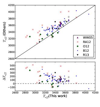
Figure 14: Upper panel: $T_{eff}$-$T_{eff}$ plot comparing the values of this work, taken from the selected sample, against others in the literature. The solid black line depicts the identity line; Lower panel: Comparison plot residuals. The dashed black line marks the zero point of our calibration.

From Figure 14 and Table 9 we observe a good agreement with the results from Woolf & Wallerstein (2005) where we obtain a low dispersion and offset. However, we only have 5 stars in common with them, and they occupy a very narrow region of the T${{}_{e}ff}$ range, around 3500 K. Our results also match well the BT-SETTL based work of Rajpurohit et al. (2013a). However, when we look at the results of the full sample we observe a significant increase in the $rms$ of Rajpurohit et al. (2013a), and we also witness a considerable dispersion with Rojas-Ayala et al. (2012) in both samples. The Önehag et al. (2012) and Boyajian et al. (2012) determinations tend to converge with ours as the $T_{eff}$ increases. We also note a systematic underestimation of our values of temperature in general that increases below 3200K. The Önehag et al. (2012) determinations have the smallest offset, but this result is expected since they use the same reference $T_{eff}$ calibration as we do. When we consider the full sample we observe that the $rms$ and offset do not change considerably, except in the case of Rajpurohit et al. (2013a). Finally, we calculated linear fits for the different $T_{eff}$ methods, where $T_{eff}$ (This work) = $aT_{eff}$ (Others) + $b$. The only exception concerns Woolf & Wallerstein (2005), because the 5 stars we have in common only cover a very narrow range in the effective temperature region. The coefficients $a$, $b$ and respective uncertainties are reported in Table 10.

Table 10: Linear fit coefficients for each $T_{eff}$ method

$T_{eff}$ method	$a$	$b$
Rojas-Ayala et al. (2012)	0.840$\pm$0.158	315$\pm$555
Önehag et al. (2012)	1.663$\pm$1.060	-2250$\pm$3499
Mann et al. (2013b)	0.643$\pm$0.184	1149$\pm$663
Boyajian et al. (2012)	1.079$\pm$0.098	-409$\pm$349
Rajpurohit et al. (2013a)	0.745$\pm$0.171	798$\pm$603

4 Discussion

In this paper we present a new high-precision technique to calculate metallicities and effective temperatures for M dwarfs. Within the activity and S/N limits of our method, we achieve a $rms$ of 0.08 dex for metallicity and 91 K for effective temperature. Alternatively we obtain a RMSE_V value of 0.12 dex for [Fe/H] and 293 K for $T_{eff}$. A bootstrap resampling was also conducted, showing a variation of the $rms$ of [Fe/H] and $T_{eff}$ of the order of $\pm$ 0.01 dex and $\pm$ 13 K respectively. Our technique is available for download at http://www.astro.up.pt/resources/mcal. The procedure to use our method is detailed in this webpage as well as in the Annex. A test of the behaviour of the technique as a function of the resolution and S/N was also performed. We estimate that our method behaves properly down to R = 40.000 and S/N = 25, after correcting the observed trends. We also validated our results against a sample of stars in common with SOPHIE high resolution spectra.

To have a measure of the accuracy of our method, we tested it against several studies from the literature. Most studies agree well with our [Fe/H] determinations, and the offset is almost always below the precision of the method. For $T_{eff}$ however, the same agreement could not be met. Despite reaching a good agreement with the results of Woolf & Wallerstein (2005), and Rajpurohit et al. (2013a), that use synthetic spectra from the latest BT-SETTL models, the dispersion as well as the systematics between our determinations and the other works is considerable and beyond the calibration errors. Further studies are needed to investigate the nature of these systematics.

Table 11: Full HARPS M dwarf GTO sample. Sorted by right ascension.

star	$\alpha$ (2000)	$\delta$ (2000)	S/N	$\log{L_{H_{\alpha}}/L_{bol}}$	$H\alpha(GdS)$	[Fe/H]N13	[Fe/H]	$\sigma$[Fe/H]	$T_{eff}$	$\sigma T_{eff}$
	[hour]	[deg]				[dex]	[dex]	[dex]	[K]	[K]
Gl1	00:05:25	-37:21:23	870	-4.88	0.01	-0.45	-0.45	0.09	3567	110
GJ10021	00:06:44	-07:32:23	21	-	0.05	-0.19	-0.27	0.20	2718	150
Gl12	00:15:49	+13:33:17	46	-	0.03	-0.34	-0.29	0.09	3239	110
LHS1134	00:43:26	-41:17:36	35	-	0.03	-0.10	-0.13	0.09	2950	110
Gl54.1	01:12:31	-17:00:00	107	-4.07	0.18	-0.40	-0.38	0.09	3088	110
L707-74	01:23:18	-12:56:23	33	-	0.03	-0.35	-0.38	0.09	3353	110
Gl87	02:12:21	+03:34:30	281	-4.88	0.02	-0.31	-0.32	0.09	3555	110
Gl105B	02:36:16	+06:52:12	143	-	0.02	-0.02	-0.02	0.09	2894	110
CD-44-836A	02:45:11	-43:44:30	68	-	0.13	-0.08	-0.07	0.09	3032	110
HIP12961	02:46:43	-23:05:12	384	-	0.07	0.22	0.22	0.09	3823	110
LHS1481	02:58:10	-12:53:06	65	-	0.02	-0.72	-0.76	0.09	3510	110
LP771-95A	03:01:51	-16:35:36	109	-	0.02	-0.34	-0.34	0.09	3236	110
LHS15132	03:11:36	-38:47:17	26	-4.93	0.03	-0.11	-	-	3197	110
GJ1057	03:13:23	+04:46:30	28	-	0.05	0.10	-0.10	0.09	2916	110
Gl145	03:32:56	-44:42:06	93	-4.89	0.04	-0.28	-0.28	0.09	3270	110
GJ1061	03:36:00	-44:30:48	28	-	0.07	-0.08	-0.09	0.09	2882	110
GJ1065	03:50:44	-06:05:42	38	-4.93	0.03	-0.22	-0.23	0.09	3062	110
GJ163	04:09:16	-53:22:25	312	-	0.02	0.05	0.07	0.09	3276	110
GJ10681	04:10:28	-53:36:06	21	-	0.04	-0.30	-0.43	0.20	2887	150
Gl166C1	04:15:22	-07:39:23	82	-3.95	0.29	0.08	-0.12	0.20	3018	150
Gl176	04:42:56	+18:57:29	576	-	0.06	-0.01	-0.01	0.09	3355	110
GJ179	04:52:06	+06:28:36	999	-	0.05	0.11	0.12	0.09	3086	110
LHS1723	05:01:57	-06:56:47	62	-4.51	0.16	-0.25	-0.24	0.09	3167	110
LHS1731	05:03:20	-17:22:23	79	-4.9	0.03	-0.26	-0.19	0.09	3273	110
Gl191	05:11:40	-45:01:06	788	-	0.00	-0.88	-0.85	0.09	3510	110
Gl203	05:28:00	+09:38:36	68	-4.93	0.03	-0.25	-0.22	0.09	3138	110
Gl205	05:31:27	-03:40:42	1430	-4.88	0.09	0.22	0.19	0.09	3670	110
Gl213	05:42:09	+12:29:23	105	-4.94	0.01	-0.11	-0.11	0.09	3082	110
Gl229	06:10:34	-21:51:53	727	-4.87	0.07	-0.01	-0.03	0.09	3633	110
HIP31293	06:33:43	-75:37:47	147	-	0.05	-0.04	-0.05	0.09	3288	110
HIP31292	06:33:47	-75:37:30	125	-	0.04	-0.10	-0.06	0.09	3184	110
G108-21	06:42:11	+03:34:53	56	-	0.03	-0.01	-0.02	0.09	3186	110
Gl250B	06:52:18	-05:11:24	167	-	0.05	-0.10	-0.08	0.09	3453	110
Gl273	07:27:24	+05:13:30	644	-	0.02	-0.01	-0.01	0.09	3090	110
LHS1935	07:38:41	-21:13:30	77	-4.9	0.03	-0.24	-0.22	0.09	3181	110
Gl2851	07:44:40	+03:33:06	85	-3.48	0.90	0.18	0.27	0.20	2946	150
Gl299	08:11:57	+08:46:23	69	-4.75	0.04	-0.50	-0.53	0.09	3373	110
Gl300	08:12:41	-21:33:12	189	-4.94	0.05	0.14	0.13	0.09	2841	110
GJ2066	08:16:08	+01:18:11	196	-	0.03	-0.18	-0.17	0.09	3421	110
GJ317	08:40:59	-23:27:23	131	-	0.07	0.21	0.22	0.09	3106	110
GJ1123	09:17:05	-77:49:17	28	-	0.04	0.20	0.15	0.09	2779	110
Gl341	09:21:38	-60:16:53	471	-	0.05	-0.13	-0.14	0.09	3575	110
GJ1125	09:30:44	+00:19:18	110	-	0.02	-0.11	-0.09	0.09	3112	110
Gl357	09:36:02	-21:39:42	258	-	0.01	-0.34	-0.30	0.09	3344	110
Gl358	09:39:47	-41:04:00	295	-4.44	0.14	-0.01	-0.01	0.09	3178	110
Gl367	09:44:30	-45:46:36	352	-4.88	0.04	-0.07	-0.07	0.09	3394	110
GJ1129	09:44:48	-18:12:48	44	-4.94	0.03	0.07	0.05	0.09	3017	110
Gl382	10:12:17	-03:44:47	532	-4.89	0.08	0.04	0.02	0.09	3401	110
Gl3881	10:19:36	+19:52:12	589	-3.8	0.40	0.07	0.12	0.20	3171	150
Gl393	10:28:55	+00:50:23	464	-4.83	0.04	-0.22	-0.20	0.09	3431	110
LHS2881	10:44:32	-61:11:35	19	-	0.03	-0.60	-0.55	0.20	2760	150
Gl402	10:50:52	+06:48:30	70	-	0.04	0.06	0.03	0.09	2943	110
Gl4061	10:56:29	+07:00:54	36	-	0.85	0.18	0.19	0.20	2523	150
GJ3634	10:58:35	-31:08:38	204	-	0.03	-0.10	-0.07	0.09	3405	110
Gl413.1	11:09:31	-24:36:00	279	-4.88	0.03	-0.12	-0.10	0.09	3394	110
Gl433	11:35:27	-32:32:23	599	-	0.03	-0.17	-0.17	0.09	3480	110
Gl436	11:42:11	+26:42:23	573	-	0.02	-0.06	-0.03	0.09	3354	110
Gl438	11:43:20	-51:50:23	254	-4.82	0.02	-0.39	-0.36	0.09	3505	110
Gl447	11:47:44	+00:48:16	133	-	0.03	-0.18	-0.17	0.09	3036	110
Gl465	12:24:53	-18:14:30	191	-4.88	0.01	-0.66	-0.62	0.09	3472	110
Gl479	12:37:53	-52:00:06	468	-4.88	0.09	0.02	0.01	0.09	3218	110
LHS337	12:38:50	-38:22:53	60	-4.97	0.03	-0.25	-0.27	0.09	3007	110
Gl480.1	12:40:46	-43:34:00	77	-	0.03	-0.48	-0.48	0.09	3211	110
Gl486	12:47:57	+09:45:12	70	-	0.02	0.06	0.03	0.09	2941	110
Gl514	13:30:00	+10:22:36	433	-4.91	0.04	-0.16	-0.16	0.09	3526	110
Gl526	13:45:44	+14:53:30	729	-5.02	0.03	-0.20	-0.22	0.09	3515	110
Gl536	14:01:03	-02:39:18	390	-4.88	0.05	-0.12	-0.14	0.09	3525	110
Gl5511	14:29:43	-62:40:47	291	-	0.42	-0.00	0.16	0.20	2654	150
Gl555	14:34:17	-12:31:06	107	-	0.03	0.17	0.14	0.09	2839	110
Gl569A	14:54:29	+16:06:04	182	-4.3	0.23	-0.08	-0.06	0.09	3289	110
Gl581	15:19:26	-07:43:17	773	-	0.01	-0.21	-0.20	0.09	3248	110
Gl588	15:32:13	-41:16:36	602	-4.89	0.03	0.07	0.06	0.09	3291	110
Gl618A	16:20:04	-37:31:41	255	-4.88	0.03	-0.08	-0.06	0.09	3200	110
Gl628	16:30:18	-12:39:47	451	-	0.03	-0.02	-0.02	0.09	3057	110
Gl643	16:55:25	-08:19:23	83	-	0.02	-0.28	-0.26	0.09	3102	110
GJ1214	17:15:19	+04:57:50	999	-	0.04	0.06	0.05	0.09	2817	110
Gl667C	17:18:58	-34:59:42	1025	-4.88	0.02	-0.53	-0.50	0.09	3445	110
Gl674	17:28:40	-46:53:42	686	-4.89	0.06	-0.25	-0.23	0.09	3334	110
GJ676A	17:30:11	-51:38:13	432	-	0.06	0.25	0.26	0.09	4071	110
Gl678.1A	17:30:22	+05:32:53	387	-4.82	0.05	-0.11	-0.14	0.09	3591	110
Gl680	17:35:13	-48:40:53	363	-4.88	0.03	-0.22	-0.19	0.09	3390	110
Gl682	17:37:03	-44:19:11	177	-4.93	0.04	0.11	0.10	0.09	2912	110
Gl686	17:37:53	+18:35:30	328	-	0.02	-0.37	-0.35	0.09	3493	110
Gl693	17:46:35	-57:19:11	133	-	0.03	-0.30	-0.28	0.09	3232	110
Gl699	17:57:49	+04:41:36	496	-	0.01	-0.52	-0.51	0.09	3338	110
Gl701	18:05:07	-03:01:53	520	-	0.04	-0.27	-0.27	0.09	3510	110
GJ12241	18:07:33	-15:57:47	35	-3.97	0.27	-0.10	-0.25	0.20	2860	150
G141-291	18:42:44	+13:54:17	24	-	0.26	0.09	-0.08	0.20	3011	150
Gl7291	18:49:49	-23:50:12	135	-3.77	0.31	-0.10	-0.40	0.20	3058	150
GJ12321	19:09:51	+17:40:07	24	-	0.05	0.14	0.03	0.20	2893	150
Gl752A	19:16:55	+05:10:05	535	-	0.04	0.06	0.05	0.09	3339	110
Gl754	19:20:48	-45:33:30	80	-	0.03	-0.17	-0.14	0.09	3005	110
GJ1236	19:22:03	+07:02:36	53	-	0.03	-0.42	-0.47	0.09	3280	110
GJ1256	20:40:34	+15:29:57	32	-	0.06	0.10	0.06	0.09	2853	110
Gl8031,3	20:45:10	-31:20:30	202	-	0.40	0.32	-	-	3430	150
LHS3583	20:46:37	-81:43:12	69	-	0.03	-0.18	-0.22	0.09	3236	110
LP816-60	20:52:33	-16:58:30	97	-	0.04	-0.06	-0.07	0.09	2960	110
Gl832	21:33:34	-49:00:36	925	-	0.03	-0.19	-0.17	0.09	3446	110
Gl846	22:02:10	+01:24:00	643	-4.82	0.07	0.06	0.01	0.09	3588	110
LHS3746	22:02:29	-37:04:54	71	-	0.03	-0.15	-0.13	0.09	3013	110
Gl849	22:09:40	-04:38:30	410	-	0.03	0.24	0.22	0.09	3143	110
GJ1265	22:13:42	-17:41:12	28	-	0.04	-0.09	-0.20	0.09	2941	110
LHS37991	22:23:07	-17:36:23	25	-	0.36	0.18	0.10	0.20	2820	150
Gl876	22:53:17	-14:15:48	554	-	0.03	0.15	0.14	0.09	2954	110
Gl877	22:55:46	-75:27:36	369	-	0.03	-0.01	-0.00	0.09	3266	110
Gl880	22:56:35	+16:33:12	351	-	0.06	0.07	0.03	0.09	3602	110
Gl887	23:05:52	-35:51:12	1434	-	0.04	-0.24	-0.24	0.09	3507	110
LHS543	23:21:37	+17:17:25	81	-4.94	0.04	0.25	0.23	0.09	2872	110
Gl908	23:49:13	+02:24:06	845	-	0.02	-0.44	-0.44	0.09	3511	110
LTT9759	23:53:50	-75:37:53	168	-	0.07	0.21	0.17	0.09	3326	110
1 Active star or star with S/N $\leq$ 25. The [Fe/H] and $T_{eff}$ were calculated using the original photometric calibrations.
2 LHS 1513 is a metal poor star outside the calibration region of Neves et al. (2012).
3 Gl 803 is a young, metal rich star outside the calibration region of Neves et al. (2012).

Table 11: continued.

Table 12: Comparison of our parameters with other results from the literature for the stars in common. Sorted by right ascension.

star	Sample	[Fe/H]											$T_{eff}$
		This work	B05	SL10	J12	WW05	RA12	O12	T12	EN13	M13a	M13b	This work	WW05	RA12	O12	B12	M13a	M13b	R13
Gl1	Y	-0.45	-0.49	-0.46	-0.3	-	-	-	-	-	-	-	3567	-	-	-	3541	-	-	-
Gl12	N	-0.29	-	-	-	-	-	-	-	-0.17	-	-	3239	-	-	-	-	-	-	-
Gl54.1	Y	-0.38	-0.11	-0.55	0.05	-	-	-	-	-	-	-	3088	-	-	-	-	-	-	3100
L707-74	N	-0.38	-	-	-	-	-	-	-	-	-	-	3353	-	-	-	3324	-	-	-
Gl87	Y	-0.32	-0.37	-0.3	-0.52	-	-	-	-	-	-	-	3555	-	-	-	3584	-	-	3600
Gl105B	Y	-0.02	-0.15	-0.09	-0.26	-	-	-0.06	-	-	-0.32	-	2894	-	-	3261	-	3505	-	-
HIP12961	Y	0.22	-0.22	-0.1	-0.44	-	0.01	-	-	-	-	-	3823	-	3838	-	4035	-	-	-
LHS1481	N	-0.76	-	-	-	-	-	-	-	-	-	-	3510	-	-	-	3306	-	-	-
LP771-95A	Y	-0.34	-0.08	0.07	-0.17	-	-	-	-	-	-	-	3236	-	-	-	-	-	-	-
GJ1057	N	-0.1	-	-	-	-	-	-	-	0.24	-	-	2916	-	-	-	-	-	-	2900
Gl145	N	-0.28	-	-	-	-	-	-	-	-	-	-	3270	-	-	-	3373	-	-	-
GJ1065	N	-0.23	-	-	-	-	-	-	-	-	-	-	3062	-	-	-	-	-	-	3200
GJ163	Y	0.07	-0.06	0.07	-0.13	-	-	-	-	-	-	-	3276	-	-	-	3475	-	-	-
Gl176	Y	-0.01	-0.0	0.13	-0.05	-	0.15	0.04	-	-	-	-	3355	-	3581	3361	3527	-	-	-
GJ179	Y	0.12	0.05	0.27	0.14	-	0.23	-	0.19	-	-	-	3086	-	3424	-	-	-	-	-
LHS1723	N	-0.24	-	-	-	-	-0.06	-	-	-	-	-	3167	-	3054	-	-	-	-	-
LHS1731	N	-0.19	-	-	-	-	-	-	-	-	-	-	3273	-	-	-	3355	-	-	-
Gl191	Y	-0.85	-0.97	-1.07	-0.5	-0.99	-	-	-	-	-	-	3510	3570.0	-	-	3716	-	-	-
Gl203	N	-0.22	-	-	-	-	-	-	-	-0.21	-	-	3138	-	-	-	-	-	-	-
Gl205	Y	0.19	0.2	0.33	0.07	0.21	0.35	-	-	-	-	0.49	3670	3760.0	4012	-	3709	-	3850	-
Gl213	Y	-0.11	-0.21	-0.24	-0.33	-	-0.25	-	-	-	-	-	3082	-	3167	-	-	-	-	-
Gl229	Y	-0.03	-0.05	0.07	0.0	-	-	-	-	-	-	-	3633	-	-	-	3672	-	-	3700
HIP31293	Y	-0.05	-0.01	0.13	0.01	-	-	-	-	-	-	-	3288	-	-	-	3441	-	-	-
HIP31292	Y	-0.06	-0.18	-0.1	0.04	-	-	-	-	-	-	-	3184	-	-	-	-	-	-	-
G108-21	N	-0.02	-	-	-	-	-	-	-	-0.01	-	-	3186	-	-	-	3415	-	-	-
Gl250B	Y	-0.08	-0.14	-0.04	-0.04	-	0.01	-0.05	-0.02	-	-0.24	-	3453	-	3569	3376	3511	3459	-	-
Gl273	Y	-0.01	-0.16	-0.07	0.08	-	-0.17	-	-	-0.04	-	-	3090	-	3293	-	-	-	-	-
LHS1935	N	-0.22	-	-	-	-	-	-	-	-	-	-	3181	-	-	-	3372	-	-	-
Gl299	N	-0.53	-	-	-	-	-0.46	-	-	-0.56	-	-	3373	-	3021	-	-	-	-	-
Gl300	Y	0.13	-0.03	0.17	0.25	-	-	-	-	-	-	-	2841	-	-	-	-	-	-	-
GJ2066	Y	-0.17	-0.15	-0.05	-0.04	-	-	-	-	-0.11	-	-	3421	-	-	-	3501	-	-	-
GJ1123	N	0.15	-	-	-	-	-	-	-	-	-	-	2779	-	-	-	-	-	-	3100
Gl341	Y	-0.14	-0.21	-0.11	-0.18	-	-	-	-	-	-	-	3575	-	-	-	3694	-	-	-
GJ1125	Y	-0.09	-0.21	-0.15	-0.06	-	-	-	-	-	-	-	3112	-	-	-	-	-	-	-
Gl357	Y	-0.3	-0.37	-0.35	-0.01	-	-	-	-	-	-	-	3344	-	-	-	3429	-	-	3500
Gl358	Y	-0.01	0.01	0.17	-0.02	-	-	-	-	-	-	-	3178	-	-	-	3425	-	-	-
Gl367	Y	-0.07	-0.08	0.03	-0.1	-	-	-	-	-	-	-	3394	-	-	-	3538	-	-	-
Gl382	Y	0.02	0.03	0.16	-0.01	-	-	-	-	-	-	-	3401	-	-	-	3584	-	-	3700
Gl393	Y	-0.2	-0.15	-0.06	-0.02	-	-	-	-	-0.18	-	-	3431	-	-	-	3475	-	-	3500
Gl402	N	0.03	-	-	-	-	0.2	-	-	-	-	-	2943	-	3334	-	-	-	-	-
GJ3634	Y	-0.07	-0.08	0.04	0.1	-	-	-	-	-	-	-	3405	-	-	-	3495	-	-	-
Gl413.1	Y	-0.1	-0.15	-0.06	-0.06	-	-	-	-	-	-	-	3394	-	-	-	3532	-	-	-
Gl433	Y	-0.17	-0.21	-0.12	-0.12	-	-	-	-	-	-	-	3480	-	-	-	3560	-	-	3600
Gl436	Y	-0.03	-0.05	0.07	-0.11	-	0.04	0.08	0.01	0.02	-	0.01	3354	-	3469	3263	3469	-	3520	-
Gl438	Y	-0.36	-0.39	-0.34	-0.24	-	-	-	-	-	-	-	3505	-	-	-	3562	-	-	-
Gl447	Y	-0.17	-0.14	-0.26	0.09	-	-0.01	-	-	-	-	-	3036	-	3065	-	-	-	-	-
Gl465	Y	-0.62	-0.56	-0.66	-0.31	-	-	-	-	-	-	-	3472	-	-	-	3395	-	-	3500
Gl479	Y	0.01	0.01	0.16	-0.03	-	-	-	-	-	-	-	3218	-	-	-	3449	-	-	-
Gl480.1	N	-0.48	-	-	-	-	-	-	-	-	-	-	3211	-	-	-	3257	-	-	-
Gl486	N	0.03	-	-	-	-	-	-	-	0.03	-	-	2941	-	-	-	-	-	-	3300
Gl514	Y	-0.16	-0.16	-0.06	-0.11	-	-	-	-	-	-	-	3526	-	-	-	3624	-	-	-
Gl526	Y	-0.22	-0.22	-0.13	-0.26	-0.1	-0.3	-	-	-	-	-0.31	3515	3650.0	3642	-	3585	-	3646	-
Gl536	Y	-0.14	-0.21	-0.12	-0.22	-	-	-	-	-	-	-	3525	-	-	-	3647	-	-	-
Gl555	Y	0.14	0.0	0.23	0.26	-	0.22	-	-	-	-	-	2839	-	3288	-	-	-	-	-
Gl569A	Y	-0.06	-0.01	0.12	0.04	-	-	-	-	-	-	-	3289	-	-	-	3495	-	-	-
Gl581	Y	-0.2	-0.22	-0.17	0.08	-	-0.1	-0.15	-0.06	-	-	-0.15	3248	-	3534	3308	-	-	3487	-
Gl588	Y	0.06	0.02	0.16	0.11	-	-	-	-	-	-	-	3291	-	-	-	3517	-	-	-
Gl618A	Y	-0.06	-0.11	0.01	-0.03	-	-	-	-	-	-	-	3200	-	-	-	3431	-	-	-
Gl628	Y	-0.02	-0.11	0.02	0.14	-	-0.02	-	-	-	-	-	3057	-	3380	-	-	-	-	-
Gl643	N	-0.26	-	-	-	-	-0.22	-	-	-	-	-	3102	-	3376	-	-	-	-	-
GJ1214	Y	0.05	-0.01	0.13	0.51	-	0.2	-	-	0.28	-	-	2817	-	3245	-	-	-	-	-
Gl667C	Y	-0.5	-0.59	-0.64	-0.23	-	-	-	-	-	-	-	3445	-	-	-	3500	-	-	-
Gl674	Y	-0.23	-0.25	-0.19	-0.0	-	-	-0.11	-	-	-	-	3334	-	-	3305	3408	-	-	-
GJ676A	Y	0.26	0.12	0.21	-0.11	-	-	-	-	-	-	-	4071	-	-	-	3931	-	-	-
Gl678.1A	Y	-0.14	-0.2	-0.1	-0.3	-	-	-	-	-	-	-	3591	-	-	-	3712	-	-	-
Gl680	Y	-0.19	-0.09	0.03	-0.12	-	-	-	-	-	-	-	3390	-	-	-	3475	-	-	-
Gl682	Y	0.1	0.0	0.23	0.39	-	-	-	-	-	-	-	2912	-	-	-	-	-	-	-
Gl686	Y	-0.35	-0.38	-0.32	-0.38	-	-0.28	-	-	-	-	-	3493	-	3693	-	3578	-	-	-
Gl693	Y	-0.28	-0.29	-0.31	-0.02	-	-	-	-	-	-	-	3232	-	-	-	-	-	-	-
Gl699	Y	-0.51	-0.29	-0.68	-0.41	-	-0.39	-	-	-	-	-0.4	3338	-	3266	-	-	-	3238	-
Gl701	Y	-0.27	-0.26	-0.18	-0.13	-0.2	-	-	-	-	-	-	3510	3630.0	-	-	3580	-	-	-
Gl752A	Y	0.05	-0.02	0.1	0.17	-	-	-	-	-	-	-	3339	-	-	-	3551	-	-	-
GJ1236	N	-0.47	-	-	-	-	-	-	-	-0.21	-	-	3280	-	-	-	3282	-	-	-
GJ1256	N	0.06	-	-	-	-	0.2	-	-	0.26	-	-	2853	-	3080	-	-	-	-	-
LHS3583	N	-0.22	-	-	-	-	-	-	-	-	-	-	3236	-	-	-	3370	-	-	-
LP816-60	N	-0.07	-	-	-	-	0.06	-	-	-	-	-	2960	-	3405	-	-	-	-	-
Gl832	Y	-0.17	-0.23	-0.15	0.04	-	-	-	-	-	-	-	3446	-	-	-	3544	-	-	-
Gl846	Y	0.01	-0.12	-0.0	-0.13	-	-	-	-	-	-	-	3588	-	-	-	3768	-	-	-
Gl849	Y	0.22	0.21	0.42	0.25	-	0.31	0.35	0.26	-	-	-	3143	-	3601	3196	3530	-	-	-
Gl876	Y	0.14	0.04	0.28	0.33	-	0.19	-	0.18	-	-	-	2954	-	3473	-	-	-	-	-
Gl877	Y	-0.0	-0.06	0.06	-0.18	-	-	-	-	-	-	-	3266	-	-	-	3467	-	-	-
Gl880	Y	0.03	0.06	0.19	-0.18	-	-	-	-	-	-	0.21	3602	-	-	-	3626	-	3731	-
Gl887	Y	-0.24	-0.33	-0.24	-0.31	-0.22	-	-	-	-	-	-0.06	3507	3680.0	-	-	3654	-	3695	-
Gl908	Y	-0.44	-0.5	-0.45	-0.41	-	-0.59	-	-	-	-	-	3511	-	3995	-	3602	-	-	-
LTT9759	Y	0.17	0.13	0.28	0.14	-	-	-	-	-	-	-	3326	-	-	-	3593	-	-	-
References: B05 - Bonfils et al. (2005); SL10 - Schlaufman & Laughlin (2010); J12 - Johnson et al. (2012); WW05 - Woolf & Wallerstein (2005); RA12 - Rojas-Ayala et al. (2012); O12 - Önehag et al. (2012);
T12 - Terrien et al. (2012); EN13 - Newton (2013); M13a - Mann et al. (2013a); M13b - Mann et al. (2013b); B12 - Boyajian et al. (2012); R13 - Rajpurohit et al. (2013a).

Table 12: continued.

Appendix A Using the method

The code of our technique is written in python 2.7 and can be downloaded at http://www.astro.up.pt/resources/mcal. The program is very simple to use. The first step is to write the filenames of your spectra into stars.txt, replacing the two demonstration filenames, Gl105B_S1D.fits and Gl849_S1D.fits. Then, one just needs to change the startup options, described in the startup section of the file runallv1.py. Depending on the resolution and S/N of the spectra, one should use the values of Table 6 as the reference of precision of [Fe/H] and $T_{eff}$.

The compressed zip file calibrationv3.zip contains all the necessary files needed to run the program, as described in the following list:

• runallv1.py - script to run all the other programs. In the startup section one can choose to use FFT to filter high frequency noise, the file type of the input spectra (FITS or text file), and the name of the file with the full path of the spectra.

• fft_filterv1.py - function that performs the FFT filtering of the spectra. The default setting of the filter in runallv1.py is ’off’.

• int_calc_stars.py - function to calculate the pseudo EWs of the relevant lines. It uses lines.rdb as input. An output file, ew_out.npz, is also created. The function also estimates the H$\alpha$ index described by Gomes da Silva et al. (2011) and warns if the star is too active. It takes 3-5 minutes per star to calculate the EWs.

• mcalv1.npz - function that calculates the [Fe/H] and $T_{eff}$ of each star using the calibration matrix file coef_cal.npz. The output will be displayed on the screen and can also be optionally saved to a file (check the startup section of runallv1.py for details).

• stars.txt - text file with the full path of the spectra. This file should have all the spectra files for analysis.

• Gl105B_S1D.fits and Gl849_S1D.fits are two HARPS spectra that can be used to demonstrate how the program works. Their full file names appear in the file stars.txt. One should remove them from stars.txt before calibrating new stars.

References

- Allard et al. (2011) Allard, F., Homeier, D., & Freytag, B. 2011, in Astronomical Society of the Pacific Conference Series, Vol. 448, 16th Cambridge Workshop on Cool Stars, Stellar Systems, and the Sun, ed. C. Johns-Krull, M. K. Browning, & A. A. West, 91
- Allard et al. (2012) Allard, F., Homeier, D., & Freytag, B. 2012, Royal Society of London Philosophical Transactions Series A, 370, 2765
- Allard et al. (2013) Allard, F., Homeier, D., Freytag, B., et al. 2013, Memorie della Societa Astronomica Italiana Supplementi, 24, 128
- Anglada-Escudé et al. (2012) Anglada-Escudé, G., Boss, A. P., Weinberger, A. J., et al. 2012, ApJ, 746, 37
- Anglada-Escudé et al. (2013) Anglada-Escudé, G., Rojas-Ayala, B., Boss, A. P., Weinberger, A. J., & Lloyd, J. P. 2013, A&A, 551, A48
- Bean et al. (2006) Bean, J. L., Sneden, C., Hauschildt, P. H., Johns-Krull, C. M., & Benedict, G. F. 2006, ApJ, 652, 1604
- Blackwell & Shallis (1977) Blackwell, D. E. & Shallis, M. J. 1977, MNRAS, 180, 177
- Bonfils et al. (2013) Bonfils, X., Delfosse, X., Udry, S., et al. 2013, A&A, 549, A109
- Bonfils et al. (2005) Bonfils, X., Delfosse, X., Udry, S., et al. 2005, A&A, 442, 635
- Bouchy & The Sophie Team (2006) Bouchy, F. & The Sophie Team. 2006, in Tenth Anniversary of 51 Peg-b: Status of and prospects for hot Jupiter studies, ed. L. Arnold, F. Bouchy, & C. Moutou, 319–325
- Boyajian et al. (2012) Boyajian, T. S., von Braun, K., van Belle, G., et al. 2012, ApJ, 757, 112
- Burgasser et al. (2003) Burgasser, A. J., Kirkpatrick, J. D., Reid, I. N., et al. 2003, ApJ, 586, 512
- Casagrande et al. (2008) Casagrande, L., Flynn, C., & Bessell, M. 2008, MNRAS, 389, 585
- Dawson & Forbes (1992) Dawson, P. C. & Forbes, D. 1992, AJ, 103, 2063
- Fabricius et al. (2002) Fabricius, C., Høg, E., Makarov, V. V., et al. 2002, A&A, 384, 180
- Gomes da Silva et al. (2011) Gomes da Silva, J., Santos, N. C., Bonfils, X., et al. 2011, A&A, 534, A30
- Hawley et al. (1997) Hawley, S. L., Gizis, J. E., & Reid, N. I. 1997, AJ, 113, 1458
- Henden et al. (2012) Henden, A. A., Levine, S. E., Terrell, D., Smith, T. C., & Welch, D. 2012, Journal of the American Association of Variable Star Observers (JAAVSO), 40, 430
- Henden et al. (2009) Henden, A. A., Welch, D. L., Terrell, D., & Levine, S. E. 2009, in American Astronomical Society Meeting Abstracts, Vol. 214, American Astronomical Society Meeting Abstracts 214, 407.02
- Henry et al. (2006) Henry, T. J., Jao, W.-C., Subasavage, J. P., et al. 2006, AJ, 132, 2360
- Johnson & Apps (2009) Johnson, J. A. & Apps, K. 2009, ApJ, 699, 933
- Johnson et al. (2012) Johnson, J. A., Gazak, J. Z., Apps, K., et al. 2012, AJ, 143, 111
- Koen et al. (2010) Koen, C., Kilkenny, D., van Wyk, F., & Marang, F. 2010, MNRAS, 403, 1949
- Laing (1989) Laing, J. D. 1989, South African Astronomical Observatory Circular, 13, 29
- Leggett (1992) Leggett, S. K. 1992, ApJS, 82, 351
- Lépine et al. (2013) Lépine, S., Hilton, E. J., Mann, A. W., et al. 2013, AJ, 145, 102
- Mann et al. (2013a) Mann, A. W., Brewer, J. M., Gaidos, E., Lépine, S., & Hilton, E. J. 2013a, AJ, 145, 52
- Mann et al. (2013b) Mann, A. W., Gaidos, E., & Ansdell, M. 2013b, ApJ, 779, 188
- Neves et al. (2012) Neves, V., Bonfils, X., Santos, N. C., et al. 2012, a&a, 538, A25
- Neves et al. (2013) Neves, V., Bonfils, X., Santos, N. C., et al. 2013, A&A, 551, A36
- Newton (2013) Newton, E. 2013, in Protostars and Planets VI, Heidelberg, July 15-20, 2013. Poster #1K093, 93
- Önehag et al. (2012) Önehag, A., Heiter, U., Gustafsson, B., et al. 2012, A&A, 542, A33
- Perryman et al. (1997) Perryman, M. A. C., Lindegren, L., Kovalevsky, J., et al. 1997, A&A, 323, L49
- Pickles (1998) Pickles, A. J. 1998, PASP, 110, 863
- Pineda et al. (2013) Pineda, J. S., Bottom, M., & Johnson, J. A. 2013, ApJ, 767, 28
- Press et al. (1992) Press, W. H., Teukolsky, S. A., Vetterling, W. T., & Flannery, B. P. 1992, Numerical recipes in FORTRAN. The art of scientific computing
- Rajpurohit et al. (2013a) Rajpurohit, A. S., Reylé, C., Allard, F., et al. 2013a, A&A, 556, A15
- Rajpurohit et al. (2013b) Rajpurohit, A. S., Reylé, C., Schultheis, M., & Allard, F. 2013b, in SF2A-2013: Proceedings of the Annual meeting of the French Society of Astronomy and Astrophysics, ed. L. Cambresy, F. Martins, E. Nuss, & A. Palacios, 259–264
- Reiners et al. (2012) Reiners, A., Joshi, N., & Goldman, B. 2012, AJ, 143, 93
- Riedel et al. (2010) Riedel, A. R., Subasavage, J. P., Finch, C. T., et al. 2010, AJ, 140, 897
- Rojas-Ayala et al. (2010) Rojas-Ayala, B., Covey, K. R., Muirhead, P. S., & Lloyd, J. P. 2010, ApJ, 720, L113
- Rojas-Ayala et al. (2012) Rojas-Ayala, B., Covey, K. R., Muirhead, P. S., & Lloyd, J. P. 2012, ApJ, 748, 93
- Santos et al. (2004) Santos, N. C., Israelian, G., & Mayor, M. 2004, A&A, 415, 1153