Systematic analysis of Persson’s contact mechanics theory of randomly rough elastic surfaces

Abstract

We systematically check explicit and implicit assumptions of Persson’s contact mechanics theory. It casts the evolution of the pressure distribution ${\rm Pr}(p)$ with increasing resolution of surface roughness as a diffusive process, in which resolution plays the role of time. The tested key assumptions of the theory are: (a) the diffusion coefficient is independent of pressure $p$, (b) the diffusion process is drift-free at any value of $p$, (c) the point $p=0$ acts as an absorbing barrier, i.e., once a point falls out of contact, it never reenters again, (d) the Fourier component of the elastic energy is only populated if the appropriate wave vector is resolved, and (e) it no longer changes when even smaller wavelengths are resolved. Using high-resolution numerical simulations, we quantify deviations from these approximations and find quite significant discrepancies in some cases. For example, the drift becomes substantial for small values of $p$, which typically represent points in real space close to a contact line. On the other hand, there is a significant flux of points reentering contact. These and other identified deviations cancel each other to a large degree, resulting in an overall excellent description for contact area, contact geometry, and gap distribution functions. Similar fortuitous error cancellations cannot be guaranteed under different circumstances, for instance when investigating rubber friction. The results of the simulations may provide guidelines for a systematic improvement of the theory.

1 Introduction

Most natural and industrial solids have rough surfaces, with roughness that is close to self-affine and fractal, and spanning several orders of magnitude in spatial scale. Persson theory [1, 2, 3] has been shown to describe the contact mechanics of such surfaces quite well. It has been extended to also describe various other properties and phenomena, such as adhesion [4, 5, 6], plasticity [2, 7], contact stiffness [8, 9], leakage [10, 11, 12, 13], squeeze-out [14], and mixed lubrication [15, 16, 17].

Persson theory builds on quite simple and elegant statistical premises about how the pressure distribution ${\rm Pr}(p,\zeta)$ changes as the “magnification” $\zeta$ is increased, i.e., sinusoidal roughness is gradually and systematically added to an initially flat, semi-infinite surface in contact with a counter body. In its original formulation [1], the only input into the theory are experimentally measurable quantities, in particular the power spectrum of the surface roughness, the effective modulus, and the external load. In recent works [18], a “fudge parameter” of order unity is introduced. Its purpose is to make the theory reflect more accurately the relation between displacement and elastic energy when contact is partial. While Persson theory has been tested numerous times and shown to describe many interfacial properties quite accurately, only the final results of the theory have been under scrutiny. So far, no quantitative analyses have been reported in the literature to what extent the assumptions entering the theory hold and to what degree (fortuitous) cancellation of errors may be responsible for its success. Manners and Greenwood [19] raise some concerns, mainly with regards to the boundary conditions employed, but fail to investigate to what measure the assumptions influence the results.

This paper quantitatively investigates the main underlying assumptions of Persson theory, and quantifies the error each assumption introduces. We do this with high-resolution numerical simulations using the GFMD method [20, 21]. There are no adjustable parameters besides those characterizing the rough surface and the ratio of pressure and elastic modulus. The assumptions of an ideally-elastic, semi-infinite half-plane are shared by Persson theory. We can test each assumption entering the theory individually and assess its effect, which may provide guidelines as to how to correct the theory in the future.

The approach pursued in this work is to solve numerically the contact mechanics problem by sequentially increasing the magnification. During each step of including more small-scale details into the simulation, we measure the detailed evolution of the system, e.g., we compute the transition probability ${\rm Pr}(p,\zeta+\Delta\zeta|p^{\prime},\zeta)$. It states the likelihood that the pressure at a given interface point in real space changes from $p^{\prime}$ to $p$ as the magnification is increased from $\zeta$ to $\zeta+\Delta\zeta$. Another central observable is how the elastic energy is distributed among different modes (in Fourier space) as $\zeta$ changes. These results are then compared to pertinent expressions in Persson theory. Analysis of individual modes provides additional information beyond previous tests of the theory that only analyzed integrated properties, for example relative contact area [22, 23, 24, 25, 26], the mean gap [27, 3, 24, 25], the contact stiffness as a function of the applied pressure [27, 8], adhesion [28], or the correlation functions of contact and pressure [29, 30].

This work is structured as follows: in Section 2 we summarize key ingredients of Persson theory, including its main assumptions we set out to test as well as the numerical methods we use. Section 3 presents the results of our tests. We discuss our findings in Section 4.

2 Methods

In this section, we summarize the key ingredients of Persson theory and the numerical methods we use. Many controlled approximations enter both Persson theory and the numerical solutions in a similar fashion. Thus, our analysis only pertains to the accuracy of the solution of the idealized contact mechanics model and not to the accuracy of the idealizations themselves.

The idealizations used in this work are: The small-slope approximation, neglect of lateral displacements, linear elasticity, semi-infinite bodies, hard-wall interactions, and absence of adhesion, although the latter can be added to both theory and simulations [31]. In addition, we assume self-affine surface spectra, whose height profiles can be characterized as colored noise. The statistical properties of our idealized surfaces are defined by their Hurst exponent $H$, cutoff (or roll-off) wave numbers limiting the power law behavior at large and small wavelengths, respectively, and a prefactor [2].

As pointed out recently in a dimensional analysis [25], systems with a cut-off at large and small wavelengths — which we consider here — are fully defined by a small set of dimensionless numbers: (i) a dimensionless pressure $\tilde{p}_{0}=p_{0}/E^{*}\bar{g}$, where $p_{0}$ is the dimensional pressure, $E^{*}$ the effective modulus, and $\bar{g}$ the root-mean-square gradient of the surface, (ii) the Hurst exponent $H$, and (iii) the ratio of the two cut-offs at short and long wavelengths, i.e., $\epsilon_{\rm f}=\lambda_{\rm s}/\lambda_{\rm l}$. In addition, one may consider (iv) the ratio of system size ${\cal L}$ and $\lambda_{\rm l}$, which, however, is only relevant at very small loads [9], and

(v), in numerical simulations, the ratio of lattice discretization $a$ and $\lambda_{\rm s}$, which we try to keep small enough to approach the continuum limit sufficiently well.

2.1 Persson theory

The contact mechanics theory by Persson has been summarized several times [1, 32, 2], also in a previous work [25]. Here we focus on its details related to the assumptions we are going to verify.

Assume we know the pressure distribution in a contact, whose spatial features are resolved up to a magnification of $\zeta$, i.e., the spectrum of the surfaces is limited to wavevectors magnitudes $q_{\rm l}\leq q\leq\zeta q_{\rm l}$, where $q_{\rm l}=2\pi/\lambda_{\rm l}$. We could predict how the distribution changes with increasing $\zeta$ if we knew the transition probability ${\rm Pr}(p,\zeta+\Delta\zeta|p^{\prime},\zeta)$, which, as stated in the introduction, specifies the likelihood that the pressure at a given point in real space changes from $p^{\prime}$ to $p$ as the magnification is increased from $\zeta$ to $\zeta+\Delta\zeta$. By definition of the transition probability, one would obtain

$${\rm Pr}(p,\zeta+\Delta\zeta)=\int{\rm d}p^{\prime}\,{\rm Pr}(p,\zeta+\Delta\zeta|p^{\prime},\zeta){\rm Pr}(p^{\prime},\zeta).$$ (1)

The starting point of Persson theory is an approximation to this transition probability according to:

$${\rm Pr}(p,\zeta+\Delta\zeta|p^{\prime},\zeta)\approx\frac{1}{\sqrt{2\pi\Delta p^{2}}}\exp\left\{-\frac{(p-p^{\prime})^{2}}{2\Delta p^{2}}\right\}$$ (2)

with

$$\Delta p^{2}=\sum_{\zeta q_{\rm l}\leq|{\bf q}|<(\zeta+\Delta\zeta)q_{\rm l}}\left(\frac{qE^{*}}{2}\right)^{2}|\tilde{h}({\bf q})|^{2},$$ (3)

where the $\tilde{h}({\bf q})$ denote the Fourier coefficients of the (combined) surface height. The broadening of pressure $\Delta p$ is motivated from the exact expression for the broadening that would hold if an infinitesimally small, single-wave height fluctuation were added to an otherwise perfectly smooth interface under a finite normal pressure. It appears that it suffices to use a Gaussian in place of the (unknown) true broadening function, because — owing to the central limit theorem — the detailed shape of transition probabilities should become irrelevant when they are applied repeatedly a large number of times.

One problem of the Gaussian transition probability is that it also allows negative pressures. This undesired property can be avoided by interpreting the broadening of the pressure distribution function in terms of a diffusive process: each point in the interface represents a walker, the pressure could be seen as its “random location”, and magnification plays the role of time. For example, as magnification goes on, the local pressure would be expected to mount when the local height increases relative to some neighborhood with greater $\zeta$, while it would diminish in the opposite case.

The boundary condition of non-negative pressures not being allowed in the given context can be implemented within this interpretation by assuming that each walker hitting the $p=0$ boundary gets absorbed into it, that is, the walker gets lost to noncontact. The idea can be realized formally by subtracting a mirror Gaussian from the original Gaussian in (2) so that

$${\rm Pr}(p>0,\zeta+\Delta\zeta|p^{\prime},\zeta)= \frac{1}{\sqrt{2\pi\Delta p^{2}}}\times$$ (4)

$$\left[\exp\left\{-\frac{(p-p^{\prime})^{2}}{2\Delta p^{2}}\right\}-\exp\left\{-\frac{(p+p^{\prime})^{2}}{2\Delta p^{2}}\right\}\right].$$

The transition probability for negative $p$ can now be set to zero. Moreover, at $p=0$, a delta-function is placed, whose prefactor is chosen such that the integral over the complete transition probability is unity.

An interesting property of the transition probability approach is that the distribution at any given magnification $\zeta$ can be calculated from (4). This is done by summing over all $\Delta p^{2}$ contributions coming from wavevectors with $|{\bf q}|<\zeta q_{\rm l}$ into the transition matrix to yield $\Delta p^{2}_{\rm tot}(\zeta)$. Moreover, the initial condition ($\zeta=1$) for smooth interfaces is that the pressure is homogeneous across the interface when no roughness features are resolved. Thus, it can be expressed as ${\rm Pr}(p,\zeta=1)=\delta(p-p_{0})$, with $p_{0}=L/A_{0}$, where $L$ is the normal load and $A_{0}$ the nominal contact area. This leads to

$${\rm Pr}(p>0,\zeta)= \frac{1}{\sqrt{2\pi\Delta p_{\rm tot}^{2}(\zeta)}}\left[\exp\left\{-\frac{(p-p_{0})^{2}}{2\Delta p^{2}_{\rm tot}(\zeta)}\right\}\right.$$ (5)

$$\left.-\exp\left\{-\frac{(p+p_{0})^{2}}{2\Delta p^{2}_{\rm tot}(\zeta)}\right\}\right].$$

We use the variable $p$ (without subscript $0$) for microscopic pressures while $p_{0}$ refers to the “macroscopic” pressure.

In the original version of the theory, the magnification dependent relative contact area $a_{\rm r}(p_{0},\zeta)$ is obtained by integrating over the pressure distribution from infinitesimally small positive pressures to infinity, yielding

$$a_{\rm r}(p_{0},\zeta)={\rm erf}\left\{\frac{p_{0}}{\sqrt{2}\Delta p_{\rm tot}(\zeta)}\right\}.$$ (6)

In more recent versions of the theory [18], Persson introduced a correction to (3) using the argument that the broadening for partial contact is less than for full contact. This leads to a modified broadening pressure

$$\Delta p^{2}_{\rm mod}=S\{a_{\rm r}(p_{0},\zeta)\}\Delta p^{2},$$ (7)

where the “fudge factor” $S\{a_{\rm r}(p_{0},\zeta)\}$ is parameterized to match the numerical results for the pressure-dependence of the relative contact area. The following functional form has been used

$$S(p_{0},\zeta)=[\gamma+(1-\gamma)a^{2}_{\mathrm{r}}(p_{0},\zeta)],$$ (8)

with $\gamma\approx 0.42$. Thus, $S\{a_{\rm r}(p_{0},\zeta)\}$ decreases monotonically from $S\{a_{\rm r}(p_{0},\zeta)=1\}=1$ to $S\{a_{\rm r}(p_{0},\zeta)\to 0^{+}\}\approx 0.42$. This means that the modification is of order unity and thus relatively minor given that many quantities span many decades, for instance the contact area, contact stiffness, and the spatial scales of the relevant wavelengths.

With this modified broadening pressure, we cannot write down a closed-form expression for the modified version of the total pressure broadening. It now has to be determined self-consistently. However, we may still use the formulae for the (total) pressure distribution and the relative contact area, as long as we insert the corrected pressure broadening terms.

Up to this point, the uncontrolled approximations in Persson theory are: (a) the pressure broadening $\Delta p^{2}$ (and similarly $\Delta p^{2}_{\rm mod}$) entering the transition probabilities ${\rm Pr}(p,\zeta+\Delta\zeta|p^{\prime},\zeta)$ only depend on $p-p^{\prime}$ (and potentially on $a_{\rm r}$) but not on the initial pressure $p^{\prime}$ of a walker in any other form, (b) there is no drift in pressure at any value of $p^{\prime}$, neither before nor after adding the mirror Gaussian, and (c) there is no flow of the probability density at $p=0$ back to positive pressure. In the interpretation of the diffusion equation, it means that any walker gone out of contact is assumed to remain out of contact for good.

Another quantity of interest is the elastic energy stored in the interface, ${\cal E}$, which is needed, for example, in the derivation of how the contact stiffness depends on pressure. According to the original Persson work [5], the energy in a resolved mode is

$${\cal E}_{\rm P}(p_{0},{\bf q}) =\frac{E^{*}}{4}\;q\;a_{\rm r}(p_{0},q/q_{\rm l})\;|\tilde{h}({\bf q})|^{2},$$ (9)

while unresolved modes are assumed to carry no energy. In more recent work [33, 18], the elastic energy was also modified with a correction factor to read

$${\cal E}_{\rm c}(p_{0},{\bf q}) ={\cal E}_{\rm P}(p_{0},{\bf q})\,S\left\{a_{\rm r}(p_{0},q/q_{\rm l})\right\}.$$ (10)

We denote the total energies stored in the interface by

$${\cal E}_{\rm P}(p_{0}) =\sum_{\bf q}{\cal E}_{\rm P}(p_{0},{\bf q}),$$ (11a)

$${\cal E}_{\rm c}(p_{0}) =\sum_{\bf q}{\cal E}_{\rm c}(p_{0},{\bf q}).$$ (11b)

Note that the contact area only depends on the nominal external load $p_{0}$ and the magnification $\zeta=|{\bf q}|/q_{\rm l}$. Only the total sum (11a) or (11b) needs to be accurate in the calculations relating to contact stiffness and mean gap, and not each individual term of (9). It might be necessary for other applications, such as rubber friction, to impose stricter requirements. Each summand associated with a given wave vector should match, on average, the corresponding term of the exact elastic energy

$${\cal E}_{\rm exa}(p_{0},{\bf q},\zeta) =\frac{E^{*}}{4}\;q\;|\tilde{u}(p_{0},{\bf q,\zeta})|^{2},$$ (11la)

$${\cal E}_{\rm exa}(p_{0},\zeta) =\sum_{\bf q}{\cal E}_{\rm exa}(p_{0},{\bf q},\zeta),$$ (11lb)

where the $\tilde{u}(p_{0},{\bf q},\zeta)$ are the exact elastic displacements in Fourier space for a given magnification and external load $p_{0}$. Those we determine to high accuracy from numerical simulations for a given realization of surface roughness defined by the $\tilde{h}({\bf q})$.

2.2 Note on contact stiffness and Persson theory

We wish to reemphasize that the purpose of this work is to analyze the starting hypotheses of Persson theory rather than the final, experimentally measurable results arising from it. It may yet be useful to remind the reader that some of these final results are the subject of current debate, in particular how the contact stiffness $\kappa$ or the linearly related contact conductance depend on pressure. Paggi and Barber [34] pointed out that many previous works found a power law relation

$$\kappa\propto p^{\alpha}$$ (11lm)

with an exponent $\alpha<1$ in agreement with their dimensional analysis but in contradiction to a linear relation, $\alpha=1$. The latter is yielded by the original Persson theory that implicitly assumes the thermodynamic limit, and also found in continuum simulations in which self-affine roughness spreads only two decades [8, 27]. Scaling arguments proposed by Pohrt et al. [35], which are meaningful when contact lives only in a single meso-scale asperity, lead to an exponent $\alpha$ in (11lm) that solely depends on the Hurst roughness exponent via

$$\alpha=\frac{1}{1+H}.$$ (11ln)

Their own numerical results, which were based on the so-called method of dimensional reduction, could not confirm this result and instead indicated that $\alpha\approx 0.266\,(3-H)$. However, work based on accurate GFMD simulations as well as an extension of Persson theory to finite systems [9] found (11ln) to be indeed true for pressures that are so small that contact does not spread over the interface but is located within a single meso-scale asperity. For more details, we refer the reader to the original literature [34, 35, 9, 25].

2.3 Numerical methods

We use Green’s function molecular dynamics [20, 21] (GFMD) to calculate the response of an ideally-elastic solid to deformations caused by mechanical contact with a rough counter body. The solids are integrated over the $z$ coordinate and modeled as semi-infinite half-planes with hard-wall interactions in the small-slope approximation so that only normal coordinates need to be considered. The setup is thereby reduced from a three-dimensional elasticity problem with $(3{\cal L})^{3}$ independent variables to a classical boundary value problem with ${\cal L}^{2}$ grid points, where ${\cal L}$ is the linear dimension of the system. We solve it with a molecular dynamics approach in reciprocal space, in order to reduce critical slowing-down from $\Or({\cal L}^{2})$ to $\Or({\cal L}^{1/2})$. While a dynamic setup is possible, for this work we are interested mainly in the static limiting case and therefore use damped dynamics here.

The details of the method can be found in Ref. [25]. We use the parallel FFTW library [36] which scales to several thousand cores. This allows us to tackle very large systems which is necessary to cover up to $5$ decades in roughness, close to what is found in natural or industrial surfaces [37, 32, 38]. A simulation with linear size $2^{17}$ corresponds to $5\times 10^{15}$ (super-)atoms in an equivalent three-dimensional simulation. More in-depth detail can be found in the original literature [20, 21].

3 Results

3.1 Preliminary remark on relative contact area and the use of units

Before we present our tests of the assumptions made in Persson theory, we comment on the dependence of contact area on pressure and resolution, as well as on our choice for pressure. In our previous work [25], we found that few dimensionless quantities suffice to define a contact. In particular, we noticed that the contact area is essentially only a function of reduced pressure $\tilde{p}_{0}=p_{0}/E^{*}\bar{g}$ as long as the linear dimension of the system ${\cal L}$ much exceeds the large-wavelength cutoff $\lambda_{\rm l}$ and the ratio of the cutoffs at small and large wavelengths is sufficiently large. As demonstrated in figure 1, we can approximate the data from our previous work via the constitutive relation

$$a_{\rm r}\approx\{1-s(\tilde{p}_{0})\}\;{\rm erf}(c_{1}\sqrt{\pi}\tilde{p}_{0})+s(\tilde{p}_{0})\;{\rm erf}(c_{2}\sqrt{2}\tilde{p}_{0}),$$ (11lo)

with two fit parameters $c_{1}=1.075$ and $c_{2}=1.025$ being very close to unity, and using a “switching function”

$$s(\tilde{p}_{0})={\rm erf}^{2}(c_{2}\sqrt{2}\tilde{p}_{0}).$$ (11lp)

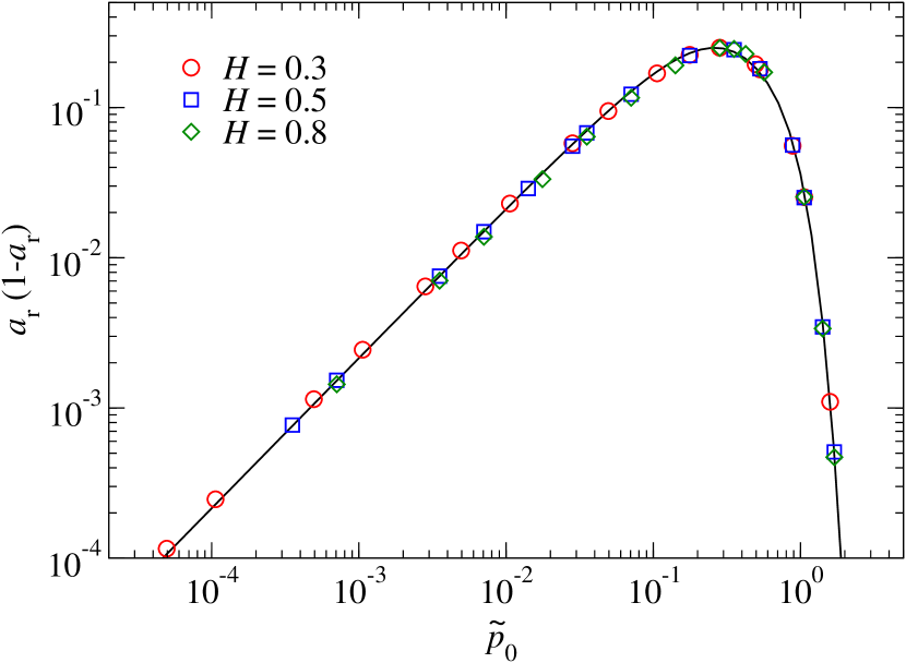
Figure 1: Representation of the relative contact area $a_{\rm r}$ as a function of the reduced pressure for three different Hurst exponents $H$, as obtained in previous GFMD simulations [25], and the approximative function, (11lo). To show the complementary relative contact area $(1-a_{\rm r})$ in the same figure, we plot $a_{\rm r}(1-a_{\rm r})$ rather than $a_{\rm r}$.

The motivation for the functional form is that $a_{\rm r}$ can be described by a single error function in the limit of low pressure and the complementary contact area by a single (complementary) error function in the limit of large $\tilde{p}_{0}$. However, the numerical coefficients to be used in the error functions at small and large pressure differ slightly. This is why we introduce a switching function that is close to zero at small $\tilde{p}_{0}$ and close to one at large $\tilde{p}_{0}$ making the first summand on the r.h.s. of (11lo) dominate the sum for small $\tilde{p}_{0}$ and the term ${\rm erf}(c_{2}\tilde{p}_{0})$ be dominant at large $\tilde{p}_{0}$. (Since the leading correction to the linear low-pressure $a_{\rm r}\propto\tilde{p_{0}}$ relation is third-order in pressure, we chose the switching function as the square of an error function.) Previous simulations found that $a_{\rm r}\propto\kappa\tilde{p}_{0}$ with $\kappa\gtrsim 2$ for $\tilde{p}_{0}\to 0$. Our approximation for $\kappa=2.15\equiv 2\,c_{1}$ is close to that value. The second term was written such that it describes the complementary contact area at large pressures in exact accordance with Persson theory for $c_{2}=1$. In agreement with a previous numerical study [26], we find that a small correction needs to be applied. In principle, the coefficients $c_{1}$ and $c_{2}$ could be optimized for different values of $H$, but for the stated numbers, $a_{\rm r}$ and $1-a_{\rm r}$ are reproduced within $O(10\%)$ accuracy for any value of $H=0.3$, $0.5$, and $0.8$ used in the simulations.

In the current work, we keep changing the resolution and thus it would not be meaningful to state absolute values of $p_{0}$. It would not be meaningful either to express pressure as $p_{0}/E^{*}\bar{g}$, because each time we increase the magnification at constant $p_{0}$, $\bar{g}$ would increase as well and thus the reduced pressure would change, although the absolute pressure $p_{0}$ would have remained unaltered. We therefore state or plot the relative contact area at a given magnification rather than $p_{0}$ or $\tilde{p}_{0}$. With the help of figure 1 or (11lo), these numbers can be easily converted into reduced pressures at that magnification. Furthermore, in most cases one can simply associate $\tilde{p}_{0}\approx E^{*}\bar{g}a_{\rm r}/2$. We choose $E^{*}\bar{g}$ as unity to nondimensionalize the pressure [25].

For microscopic, local pressures, i.e., those that hold for individual points at the interface, we use $p_{0}/a_{\rm r}$ as default unit as the latter reflects the mean pressure averaged over the contact. Thus, when identifying a walker with a pressure much less than unity, there is a large probability that it sits either close to a contact line or in a small patch bearing little load. As stated before, the variable $p$ stands for local pressures while $p_{0}$ refers to the “macroscopic” pressure.

3.2 Pressure-independent and drift-free broadening

In this section we test the first two approximations implicitly contained in Persson theory. They can be described as the following two properties of the transition probability ${\rm Pr}(p^{\prime},\zeta+\Delta\zeta|p,\zeta)$: (a) the term related to the broadening of the pressure distribution, $\Delta p^{2}$ depends only on $p-p^{\prime}$, i.e., the “diffusion coefficient”

$$D=\Delta p^{2}/\Delta\zeta$$ (11lq)

is independent of $p^{\prime}$, and (b) the transition probability induces no drift at any pressure.

In order to test these two approximations, we first ran simulations with a maximum resolved target wave number $\lambda_{\rm t}={\lambda_{\rm l}/\zeta}$ with $\zeta=63$. In these calculations, the Hurst exponent was set to $H=0.5$ and a system size of ${\cal L}=16,384$ was investigated. The pressure was chosen such that it produced a relative contact area of $0.01$ for the given magnification of $\zeta=63$. From the relaxed configurations we computed the pressure at each point at the interface and produced a pressure distribution function from it on a discretized mesh with constant spacing $\Delta p$. For selected bins with index $n$, we memorized each grid point, or walker, for which the pressure lay in the interval $n\Delta p\leq p<(n+1)\Delta p$ at $\zeta=63$. The magnification was then increased to $\zeta=63.3$ and the distribution function (of the new configuration) evaluated over the points that had been associated with the given bins at the old magnification. This yields a discretized version of the transition probability. Results are shown in figure 2.

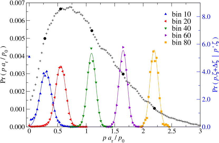
Figure 2: Original, discretized pressure distribution ${\rm Pr}(p)$, indicated by plus signs, at a magnification of $\zeta=63$. For selected bins, indicated by full circles, the transition probability ${\rm Pr}(p,\zeta+\Delta\zeta|p^{\prime},\zeta)$ is recorded for $\Delta\zeta=0.3$ (right ordinate axis). They are shown in color. Full lines represent fits to mirror Gaussians as described in the Appendix. Starting at bin 20, the difference to simple Gaussian is negligible. The heights and thus the widths of the transition probabilities turn out to depend on pressure $p$. The simulations were run with $H=0.5$ and $a_{\rm r}\approx 0.01$.

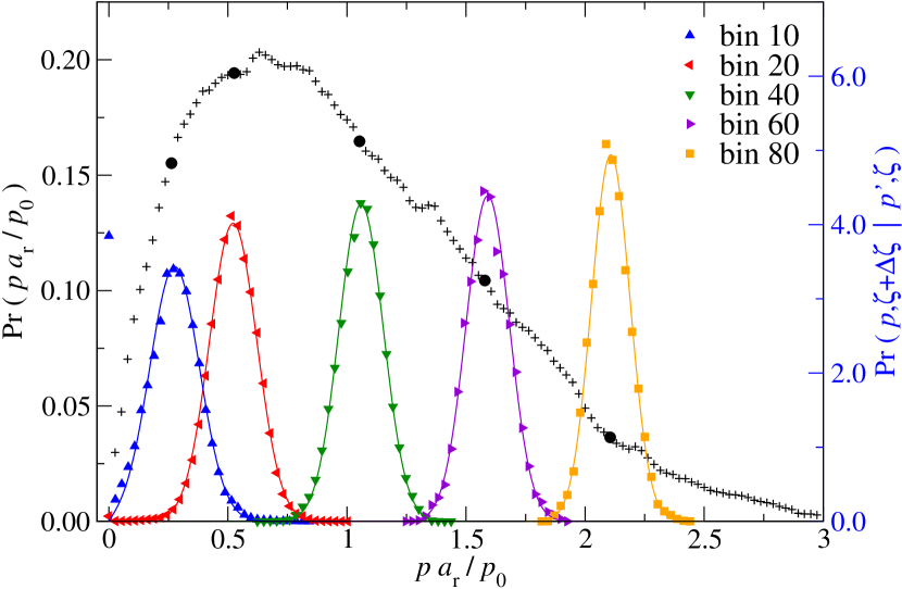
Figure 3: Similar to figure 2, except that the simulations used here were for $H=0.8$ and $a_{\rm r}\approx 0.31$, and the magnification changed from $\zeta=16$ to $\zeta=16.2$. The figures show identical trends.

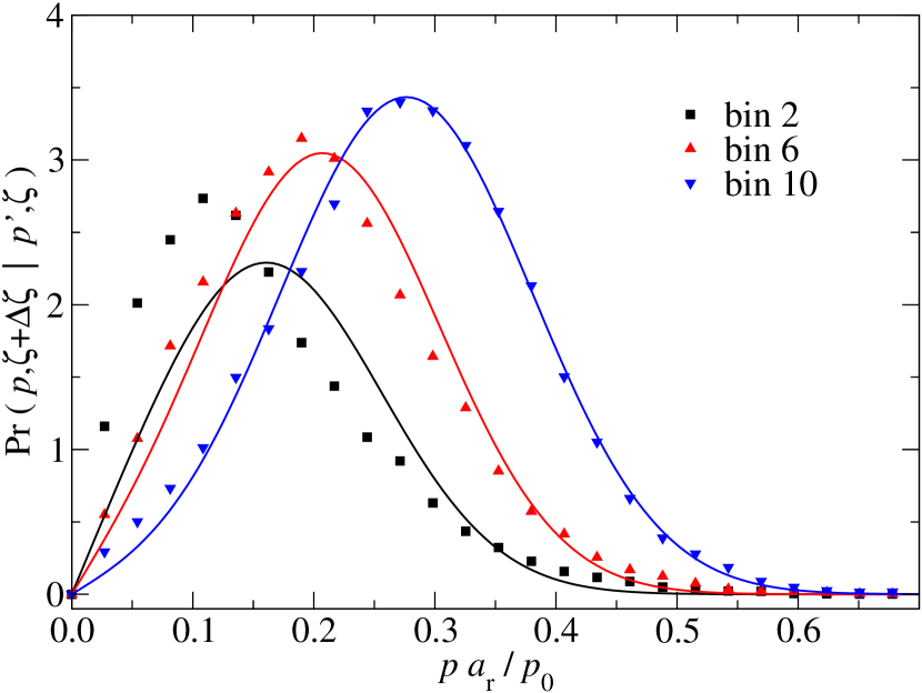
Figure 4: Pressure distribution of some low-pressure bins for $H=0.8$ and $a_{\rm r}\approx 0.31$. The singularity at $p=0$ is omitted in all cases. The mirror-Gaussian function with on-the-fly determined parameters (solid lines) only fits well as long as the broadening is smaller than the mean. Below that threshold, the description is unsuitable. It is in principle still possible to fit a mirror-Gaussian to the data (not shown), but the normalization is inconsistent. We therefore did not include bins $<8$ in our analysis.

In figure 2, the transition probabilities are described accurately by mirror Gaussians, for the bins whose mean pressure much exceeds the broadening, and information on the diffusion coefficient can be ascertained directly. For example, a systematic on-the-fly determination of the diffusion coefficient associated with one of these bins can be done by subtracting the variance obtained at the old magnification from that at the new magnification. However, special care has to be taken for the analysis of those bins representing small pressures. In A we describe how to compute drift and diffusion coefficients such that their determination is also meaningful when the mean pressure of a bin is smaller than the broadening. If the diffusion into the singularity at $p=0$ is negligible, even a simple Gaussian suffices with high accuracy.

We carried out the same analysis for $H=0.8$ and a much larger relative contact area of $a_{\rm r}\approx 0.31$. Figure 3 shows that there is no qualitative difference for the different Hurst exponents, or at different external loads.

Figure 4 shows bins for which the broadening is larger than the means. In this case, the procedure laid out in A is not suited anymore. While bin 10 is still described quite well (but not by a simple Gaussian anymore), for bin 6, only the width is still acceptable. The peak is shifted slightly. For bin 2, finally, neither the width nor peak are suitably described. We did not include any data from bins $<8$ in the following.

In order to arrive at more quantitative results, we conducted a moments analysis of the pressure distribution, as described in A, for $64$ bins, for a relative contact area of $a_{\rm r}=0.3$. The results shown in figure 5 reveal that the drift is negligible for large pressures and that the diffusion coefficient comes out as assumed in the original version of Persson theory. That means that no correction factor is required to predict the correct broadening for most values of $p$, although for $a_{\rm r}=0.3$, $S(p_{0},\zeta)$ in (8) should already be close to its minimum value $\approx 0.42$. Drift and diffusion coefficients only deviate from the prediction for $p\ll p_{0}/a_{\rm r}$, that is, at pressures much smaller than the mean pressure in the contact regions.

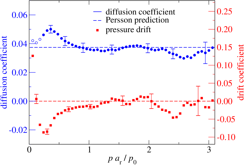
Figure 5: Diffusion (blue circles, left $y$-axis) and drift coefficients (red square, right $y$-axis), describing the evolution of the pressure distribution between a magnification of $16$ and $16.2$, at relative contact areas of $a_{\rm r}(\zeta=16)=0.2667$ and $a_{\rm r}(\zeta=16.2)=0.2662$. The shown data is averaged over four equivalent but statistically independent realizations of the surface. The dashed lines reflect assumptions made in the original version of Persson theory. Non-negligible stochastic uncertainties remain for $p\gg p_{0}/a_{\rm r}$ as revealed by the error bars. Stochastically significant discrepancies from the drift-free and the constant-diffusion-coefficient assumptions remain for pressures $p\ll p_{0}/a_{\rm r}$. These can be rationalized by assuming that low-pressure points tend to be located close to a contact line. Open symbols are from bins where the mirror-Gaussian fit function is unsuited to determine the diffusion coefficient, even though the drift in those bins is well defined.

It can be easily rationalized why the assumptions made in Persson theory hold for $p\gtrsim p_{0}/a_{\rm r}$ but not for $p\ll p_{0}/a_{\rm r}$. Walkers contributing to the histogram at pressures $p\gtrsim p_{0}/a_{\rm r}$ lie far away from any contact line and pressure gradients should usually be small. The assumption that additional roughness leads to small pressure perturbation is thus justified, certainly as long as $\lambda_{\rm l}/\zeta$ is small compared to the linear dimension of the contact patch to which this walker belongs. In contrast, walkers contributing to the histogram at $p\ll p_{0}/a_{\rm r}$ lie close to a contact line, or, more generally, close to a point or patch that risks to fall out of contact soon. Pressure gradients are high at those positions and even diverge right at the contact line (as in Hertzian contacts), which explains why the diffusion coefficient picks up at small pressures. Moreover, pressure gradients increase as the contact line is approached, which is consistent with the presence of a negative drift. If, however, a walker is extremely close to a contact line, there is a large probability that the walker jumps from contact with large pressure gradients to out-of-contact, where the pressure gradient is zero. This explains why the drift turns around in sign at extremely small pressures.

An interesting observation in figure 5 is that the pressure broadening in the contact agrees with the original, correction-parameter-free variant of Persson theory rather than with the modified version. At the same time, points fall out of contact more quickly than predicted by Persson theory because many walkers acquire a negative drift at $p<p_{0}/a_{\rm r}$. Their number is distinctly larger than of those having a positive drift so that the average contact drift coefficient

$$\bar{\mu}_{\rm c}=\frac{1}{a_{\rm r}}\int_{0^{+}}^{\infty}{\rm d}p\,{\rm Pr}(p)\mu(p)$$ (11lr)

is negative.

So far, our calculations imply that there is mean drift towards smaller pressures and an increased diffusion at small pressure as compared to the theoretical prediction. From this point of view, one would expect Persson theory to overestimate the contact area. However, the opposite is true. Thus, one must expect walker to re-enter contact upon an increase of magnification, which would counteract the large flux out of contact that is induced by large diffusion coefficients and negative drifts at small $p$. We investigate this hypothesis next.

3.3 No re-entry

One key assumptions in Persson theory is that points at the interface are seen to fall out of contact as finer details of the surface roughness are incorporated. The idea is visualized in figure 6, which shows cuts through the converged surfaces for simulations with system sizes of $4,096\times 4,096$ at five different resolutions $\zeta=\{2,4,16,64,256\}$. The cuts are at the same location for each surface. In each panel, roughness is added on successively smaller scales. Even though we did not select the location of the cut specifically for this effect, we happened to find a re-entry point.

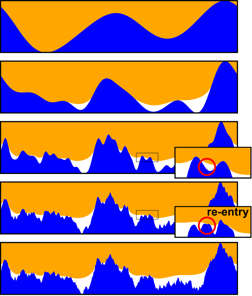
Figure 6: (Color online) Cut through a rough contact with gradually increased roughness on smaller and smaller scales. The magnification increases from top to bottom with $\zeta=\{2,4,16,64,256\}$. The top (orange) solid holds all the compliance, while the lower (blue) body contains all the roughness. The gap is kept in white. Even though the overall shape does not change at large magnification, the local topology does, and this causes re-entry of some points that had previously fallen out of contact.

A similar analysis as that for the cross section of a contact shown in figure 6 is repeated in terms of a bird’s eye view of the interface in figure 7. There we highlight areas that change from contact to non-contact and vice versa, as $\zeta$ is increased from $128$ to $129.5$. Analysis of the data reveals that the net flux to non-contact is a small fraction of $\Or(15\%)$ of the flux in either direction. The large flux of points getting back into contact supports the hypothesis that reentry distinctly increases the contact area relative to the predictions by Persson theory. The effect is sufficiently large to overcompensate the effects discussed in Section 3.2.

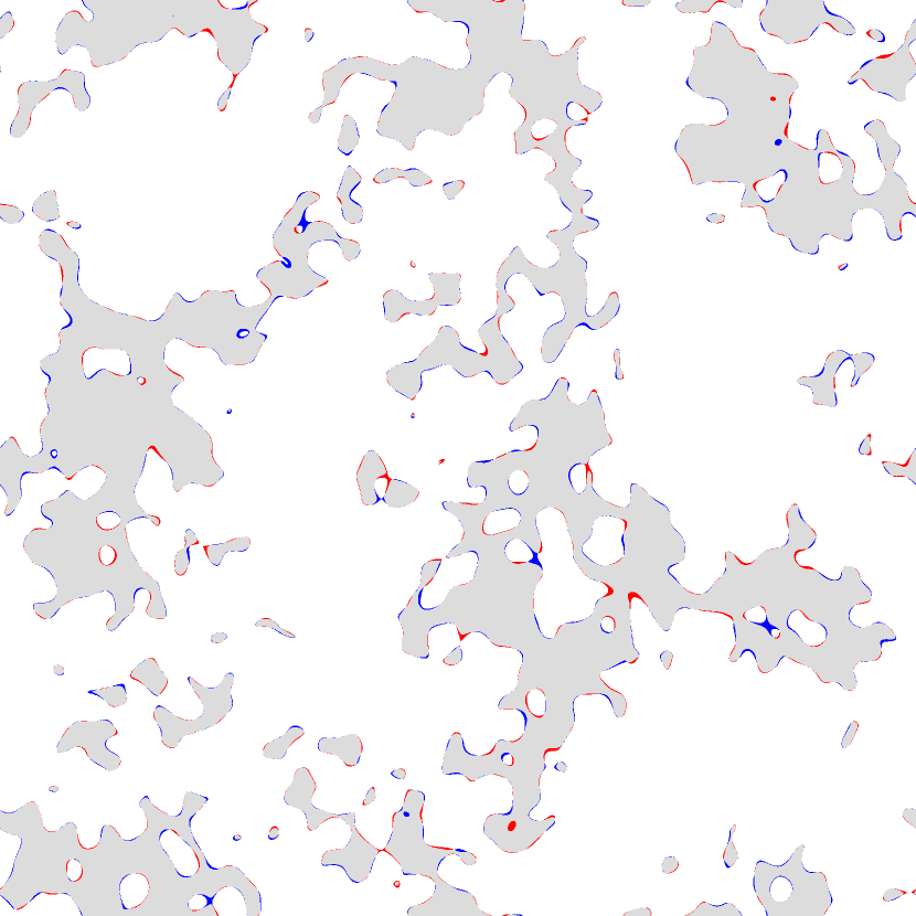
Figure 7: (Color online) Visualization of a contact geometry of a $4,096\times 4,096$ system with $H=0.8$ and a relative contact area of $a_{\rm r}=0.14$ at magnification $\zeta=129.5$. White and blue areas represent non-contact, while gray and red show contact patches. Blue and red points have changed their nature between $\zeta=128$ and $\zeta=129.5$, i.e., blue was in contact at $\zeta=128$, while red was in non-contact at the smaller magnification. Since all points are in contact when only the very longest wavelength is considered ($\zeta=1$), the red points have “reentered” contact. The relative contribution of red and blue are $0.675~{}\%$ and $0.597~{}\%$ of the apparent contact area, respectively, implying that the net flow $0.078~{}\%$ is small compared to the flux in either direction. The reentry process is not accounted for by Persson theory.

As one may expect a re-entry contact point to get out of contact soon again, it is not clear how many contact points at a given magnification are reentrant points. To answer the question how many points have ever returned to contact — or returned to non-contact — one needs to examine every single change in magnification. This is an extremely tedious and computationally expensive procedure — even for a small system, $1,024\times 1,024$ in size, with $\lambda_{\rm l}=512$ and $\lambda_{\mathrm{s}}=4$, there are a total of $\approx 4,400$ different wave numbers, each of which has to be added one-by-one, and the same number of separate simulations run, for each value of the external load. In addition, this process has to be repeated for different surfaces to ensure robust numbers. We ran a set of eight different random realizations for each pressure value of size $1,024\times 1,024$. We did not attempt to carry out this analysis for systems larger than $4,096\times 4,096$, so that the resulting percentage is still only an estimate, as the fractal limit is not reached fully. However, it does serve as an orientation — when taking into account a larger range of magnifications more points are bound to experience re-entry than for a smaller range. Nevertheless, for $a_{\rm r}=0.14$ and $H=0.8$, we find that $\approx 62\%$ of all contact points at the highest resolution have left and re-entered contact at a lower magnification. For $a_{\rm r}=0.014$, every single point in contact had lost contact at a lower magnification. Even for $a_{\rm r}=0.88$, where contact is nearly complete, the fraction is still $\approx 8\%$ and thus non-negligible. These numbers do not change if the continuum limit is approached even closer — for $\epsilon_{\rm c}=1/8$ and $1/16$, the fractions remain the same. They do not depend much on $\lambda_{\rm l}/{\cal L}$ either, and remain comparable for $\epsilon_{\rm t}=1/4$. The Hurst exponent similarly has a very minor effect; the numbers for $H=0.3$ lay within $4\%$ of those for $H=0.8$, and neither showed a dependence on $\epsilon_{\rm t}$ nor $\epsilon_{\rm c}$.

Figure 8 visualizes the reentry for a system of $2048\times 2048$ over a larger range of magnifications. All points shown in color have reentered contact in the examined range, and only $\approx 25\%$ of all points have remained in contact.

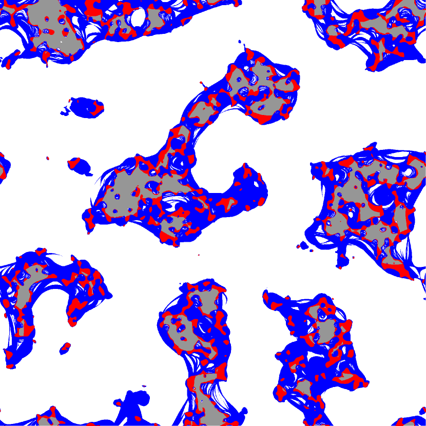
Figure 8: Similar to figure 7, except for a $2048\times 2048$ system and different initial ($\zeta=3.2$) and final ($\zeta=32$) magnifications, for which the contact areas were $a_{\rm r}=0.28$ and $a_{\rm r}=0.14$, respectively. Here, gray points have been in contact at all intermediate magnifications, and white points have either been out of contact at $\zeta=3.2$ or lost contact exactly once. In contrast, all points in color have experienced reentry between $\zeta=3.2$ and $\zeta=32$; blue points show out-of-contact reentry and red indicates contact reentry. Note that there are $3.8$ times more colored points than gray points, and of all points in contact at the final magnification, $50\%$ have experienced reentry. Sharp features all come from low magnifications where the surface changes relatively strongly with each added wave number.

To complete the analysis of reentrance, we note that figure 9 includes data for the pressure transition probability for an initial pressure of $p^{\prime}=0$, similar to our analysis for finite $p^{\prime}$. For a change from $\zeta=63$ to $\zeta=63.3$, we find about $1\%$ of all points previously in noncontact reenter contact. Such points therefore act as if they came from a “source” in the framework of the diffusion analogy, or, more precisely, as if they were reflected — potentially with a delay — by the boundary. This can affect the functional form of the pressure distribution function and lead to deviations from a linear ${\rm Pr}(p)\propto p$ dependence at small $p$, which one gets for the distribution shown in (5). In fact, preliminary results are in violation of a ${\rm Pr}(p)\propto p$ relationship.

Figure 9: Histogram of the points in the zero pressure bin at $\zeta=63$, after the magnification is increased to $\zeta=63.3$. The total transition probability is $\approx 0.01$. This means that $1\%$ of all points reenter between $\zeta=63$ and $\zeta=63.3$.

3.4 Single-mode analysis of the elastic energy

As mentioned before, the derivation of Persson theory assumes that an energy mode contains no energy until the appropriate mode of roughness is resolved. Beyond this magnification, the energy in this mode is expected remain the same when even greater wave numbers are included. For various external loads, figure 10 and 11 demonstrate that this is an oversimplification when contact is incomplete. We plot the following expression for a given target wave number $q_{\rm t}$

$${\cal E}_{\rm norm}(p_{0},q_{\rm t},\zeta) \equiv\frac{{\cal E}_{\rm exa}(p_{0},q_{\rm t},\zeta)}{{\cal E}_{\rm P}(p_{0},q_{\rm t})}$$ (11ls)

$$\approx\frac{\sum_{|{\bf q}|\approx q_{\rm t}}q\;|\tilde{u}({p_{0},\bf q,\zeta})|^{2}}{\sum_{|{\bf q}|\approx q_{\rm t}}q\;a_{\rm r}(p_{0},q_{\rm t}/q_{\rm l})\;|\tilde{h}({\bf q})|^{2}},$$

while

$${\cal E}^{\rm pred}_{\rm norm}(p_{0},q_{\rm t},\zeta) =S(p_{0},\zeta)\;\Theta(\zeta-q_{\rm t}/q_{\rm l})$$ (11lt)

is the predicted normalized energy. $\Theta(\zeta-q_{\rm t}/q_{\rm l})$ is the Heaviside step function which is zero for $\zeta<q_{\rm t}/q_{\rm l}$ and $1$ for $\zeta\geq q_{\rm t}/q_{\rm l}$. We find that each mode is partially excited already at a lower magnification than expected, and peaks at a higher magnification. Partly this is caused by averaging the contribution of a number of nearby wave numbers for reasons of reducing scatter. Another important effect should be related to the following phenomenon: The derivative of the stress becomes singular as a contact line is approached from within the contact. It then discontinuously drops to zero outside the contact, as one can readily see in the case of a Hertzian contact. This implies that the Fourier coefficients of the stress and thus the strain field must be non-zero up to (infinitely) large wavevectors as soon as there is partial contact. The corresponding amplitudes may be small, but they are non-zero.

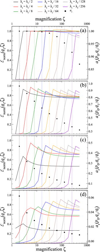
Figure 10: Normalized elastic energy, see (11ls) for system sizes of $16,384\times 16,384$ and a Hurst exponent of $H=0.8$, averaged over 8 statistically equivalent but independent random realizations. The cutoff wave numbers were $\lambda_{\rm l}=8,192$ and $\lambda_{\rm s}=8$, approximately fulfilling the thermodynamic, fractal, and continuum limits. Each panel shows the elastic energy for a different relative contact area at full resolution (top to bottom) of 0.87, 0.32, 0.083, 0.009, in a collection of nearby Fourier modes with $q_{\rm t}\approx\zeta q_{\rm l}$ normalized by the energy that they are expected to have in the original Persson theory, i.e., normalized by $a_{\rm r}(q_{\rm t}/q_{\rm l})\;E^{*}/4\sum_{|{\bf q}|\approx q_{\rm t}}q|\tilde{h}({\bf q})|^{2}$. The right ordinate axis shows the relative contact area at the given magnifications.

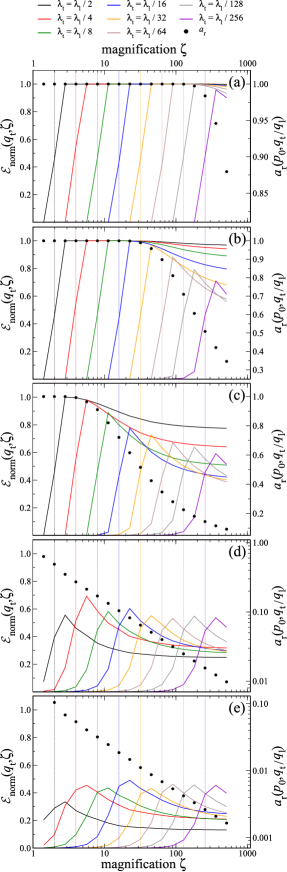
Figure 11: Similar to figure 10 but for $H=0.3$ and the contact areas (top to bottom): 0.88, 0.35, 0.093, 0.0098, 0.0017. Note that in panels (d) and (e), the axis for the contact area is logarithmic.

When the external load is very high, as is the case in figure 10a, contact remains complete up to high magnification, and (11lt) is essentially accurate. When the pressure is reduced, as in figure 10b, or, alternatively, the magnification is increased further, less energy starts to be stored in the short-wavelength modes than predicted. However, also the long-wavelength modes are populated less than anticipated. Interestingly, the energy reduction is even stronger for long wavelengths than for short wavelengths and in contradiction to the functional form of $S(p_{0},\zeta)$ in (8), as revealed by figure 10c and 10d.

Short wavelengths are populated in a way that roughly conforms with Persson theory before including the correction factor (8). However, long wavelength displacements do not appear to develop as much as expected and even appear to recede when roughness is added at large magnification and small external pressure. This effect is captured neither in the original version of Persson theory nor in the modified version.

Figure 10 and 11 seem to show a correlation between the asymptotic value that the elastic energy, normalized with Persson’s prediction, converges to, and the relative change of the relative contact area. We explore this correlation in figure 12 and 13. The fall-off of the elastic energy turns out to be linear with magnification, so we can extrapolate the curves for $\lambda_{\rm t}\geq\lambda_{\rm l}/128$ to $\zeta\longrightarrow\infty$ to determine the asymptotic value.

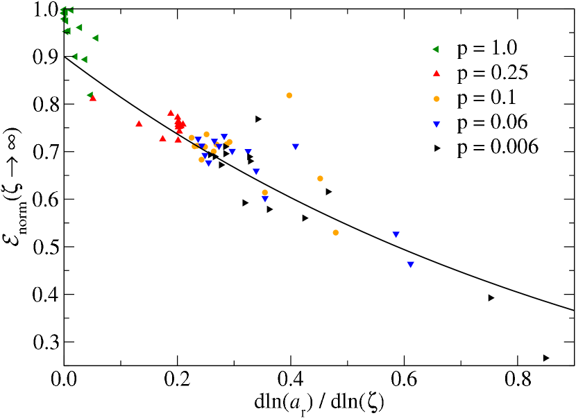
Figure 12: Asymptotic value of the ratio of elastic energy to Persson prediction for $H=0.8$ (see figure 10) versus the relative change of the relative contact area with magnification, ${\rm d}\ln a_{\rm r}/{\rm d}\ln\zeta$. Despite some scatter, a correlation is visible, of the form $0.9\,\exp(-1.0\,x)$.

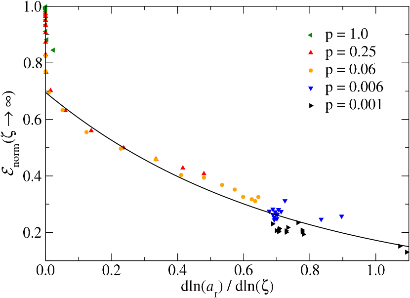
Figure 13: As figure 12, but for $H=0.3$. The correlation is not the same as for $H=0.8$, but the same form, with $0.7\,\exp(-1.4\,x)$.

Ignoring the values at full contact, there indeed is a correlation, despite some scatter, of the form $\tilde{K}_{1}\,\exp\left[-\tilde{K}_{2}\,{\rm d}\ln(a_{\rm r})/{\rm d}\ln(\zeta)\right]$. The value of the constants is not universal and changes with Hurst exponent, but — at least for the two cases we inspected — assumes values of $\Or(1)$. Further investigations are necessary.

3.5 Analysis of the integrated elastic energy

The previous section showed that the individual modes of the elastic energy do not behave as Persson theory assumes, except near perfect contact. Nevertheless the theory quite accurately predicts the relative contact area and the mean gap found in the contact between two randomly rough elastic bodies. Especially the latter depends intimately on the elastic energy — albeit not on each mode but on the total sum. Still it is not obvious that the total elastic energy is correct while each individual term is inaccurate. In this section, we examine the integrated elastic energy and compare this to the results that Persson theory posits.

In order to test the correction factor that is present in Persson theory, we calculate it numerically using

$$\widetilde{S}(p_{0},\zeta)=\frac{{\cal E}_{\rm exa}(p_{0},\zeta)-{\cal E}_{\rm exa}(p_{0},\zeta-\Delta\zeta)}{{\cal E}_{\rm P}(p_{0},\zeta)-{\cal E}_{\rm P}(p_{0},\zeta-\Delta\zeta)},$$ (11lu)

where the numerator comprises the subtraction of the total elastic energy of a simulation in which everything up to a magnification of $\zeta$ is resolved from that of a simulation with a slightly lower magnification. The denominator is the difference between (11a) for two different values of $\zeta=q/q_{\rm t}$, which leaves only terms due to the newly resolved wavelengths. We increment the resolution by the minimum amount possible for a given discretization, i.e. recompute the contact for each new wave number separately. This expression would yield the correction factor if each mode of the elastic energy were excited exactly at its appropriate resolution and remained constant with any further increase of resolution. Similarly in that case, (11ls) would yield (11lt).

The numerator varies quite substantially for different values of $q$. As a consequence $\widetilde{S}(p_{0},\zeta)$ converges very slowly, so figure 14 is the result of more than $2,400$ sets of independent random instances, for a total of about $2.9$ million simulations of size $512\times 512$. We confirmed the results with higher-resolution simulations at $N=1024$ ($95$ sets, $\sim 400,000$ simulations), and, at selected magnifications, with $N=2048$ ($\sim 100$ sets, $80,000$ simulations). The latter also include magnifications up to $\zeta=128$.

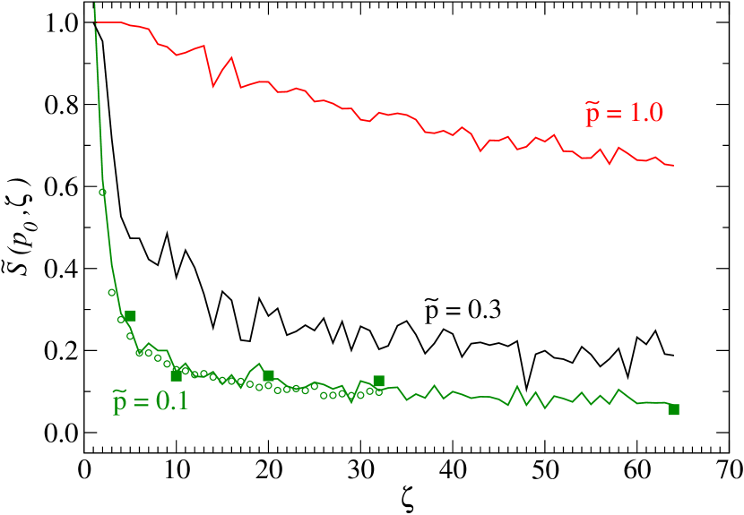
Figure 14: Incremental correction factor $\widetilde{S}(p_{0},\zeta)$, see (11lu), versus magnification, for different pressures. Solid lines are $N=1024$, while open circles ($N=512$) and filled squares ($N=2048$) are size-scaled data which shows that the values are converged. The data is averaged over between $10$ and $2,500$ different realizations of the rough surface.

Since we know from figure 10 and 11 that the individual modes of the elastic energy ${\cal E}_{\rm norm}(\zeta)$ do not behave exactly as assumed in Persson theory, (11lu) may not be an appropriate comparison. Instead, we consider the deviations of the total elastic energy with respect to the magnification and to the measured relative contact area.

$${\cal E}_{\rm norm}(p_{0},\zeta)=\frac{{\cal E}_{\rm exa}(p_{0},\zeta)}{{\cal E}_{\rm P}(p_{0},\zeta)},$$ (11lv)

The results are shown in figure 15 (varying $\zeta$ for $p_{0}={\rm const}$) and figure 16 (for $\zeta=64$, varying $p_{0}$, and therefore $a_{\rm r}$). They reveal that using (8) indeed significantly improves agreement between theory and numerical measurements compared with the original theory where $S\equiv 1$. Nevertheless, the total elastic energy is still overestimated by $\approx 10\%$ even with the more complicated functional form. At low pressures, even the correction factor is insufficient to get theory and measurement to agree.

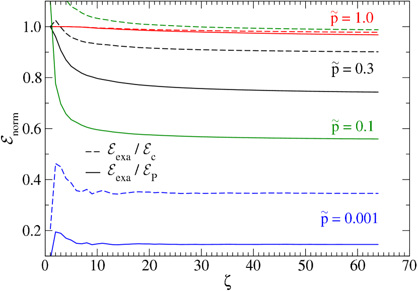
Figure 15: Integrated normalized elastic energy. The solid lines represent the original variant of Persson theory (with $S(\zeta)=1)$, while the dashed lines hold for $S$ as given in (8). For high and intermediate pressures, the corrected expression yields very good values. At $\tilde{p}=0.1$ and low magnification, the correction factor boosts the elastic energy beyond the measurement, while at even lower pressures, the result is far below the measurement. Each data set is an average over $10$ different random realizations.

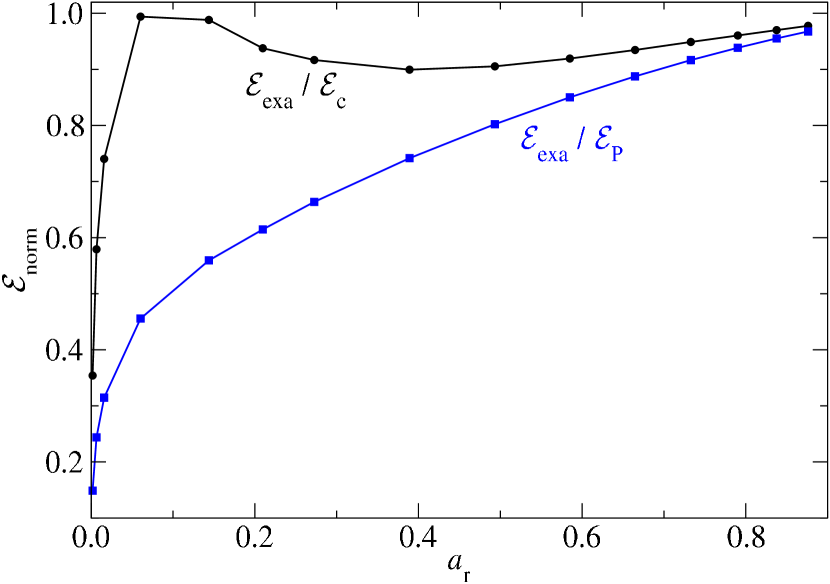
Figure 16: Similar to figure 15, except that the integrated normalized elastic energy is plotted against the relative contact area (at constant magnification $\zeta=64$). Each data set is an average over $10$ different random realizations. The correction factor works well for $a_{\rm r}\gtrsim 0.05$; at even lower pressures, the deviation from the measurement increases dramatically.

4 Conclusions

In this work, we have revealed quite significant shortcomings of the assumptions entering Persson’s contact mechanics theory. However, many errors cancel, which explains why quite a few interfacial properties are predicted very accurately by the theory. It is nevertheless not clear if all interfacial properties benefit from such cancelations so that the theory might need to be improved for some applications. For example, in the context of rubber friction or other problems involving moving interfaces, the inaccurate partitioning of energy amongst different modes might be problematic. At the current stage of development, only the net elastic energy of a relaxed configuration turns out reasonable.

Despite our criticism, we recognize Persson theory as the only theory for rough, linearly-elastic contacts that is based on controlled approximations and reveals accurate information not only on scalar numbers but also on distribution functions including contact geometry. The theory is essentially only based on directly measurable quantities and thus free of ad-hoc parameters except for one correction factor of order unity. In this work we found evidence that this correction factor is needed but has so far been implemented only heuristically. Our results indicate that the correction factor does not yield very accurate elastic energies at low pressure and moreover is sensitive to the rate at which the relative contact area decreases with increasing resolution rather than to the relative contact area itself. One reason why the gap distribution functions are nevertheless predicted quite accurately may be that for low pressures the mean gap is approximately only logarithmic in pressure [33, 18, 3, 25]. As a consequence, a change in gap is only a logarithmic function of energy so that only the order of magnitude of the energy needs to be known. For high pressures, on the other hand, Persson theory is quite accurate.

Correcting individual ingredients to the contact mechanics theory might disturb a delicate balance of error cancelations which is currently present. It might therefore be necessary to make adjustments to the elastic energy and the various aspects of the diffusion analogy simultaneously so that the predictions of the quantities tested so far do not deteriorate.

It would certainly be desirable to motivate corrections to the theory without making ad-hoc or uncontrolled assumptions. One possible avenue to derive such corrections is to consider a model in which hard-wall repulsion is replaced with smoother repulsion, such as exponential repulsion, which is more amenable to analytical calculations than (non-holonomic) hard-wall constraints. In fact, one of the authors investigated such a model [39] and proposed that stress-dependent drift arises beyond a second-order cumulant expansion of the model, which is formally equivalent to Persson theory. Pursuing such an expansion might, however, turn out tedious. The analytical expressions become increasingly involved with each added order and the next non-vanishing term for colored-noise surfaces only arises at fourth order.

Appendix A On-the-fly determination of the diffusion coefficient

The deduction of drift and diffusion coefficients from data for the transition probability, ${\rm Pr}(p,\zeta+\Delta\zeta|p^{\prime},\zeta)$, as shown in figure 2, becomes non-trivial when the magnification-induced broadening is no longer small compared to $p^{\prime}$. It is then no longer sufficient to assume that the increase of the second moment of the pressure from old to new magnification reflects the broadening. An example is the case for the distribution associated with the bin number 10 in figure 2. The reason why looking at the change in the second moment of the distribution is no longer sufficient is that some walkers belonging to bin 10 at the original magnification have fallen out of contact at the new magnification, as one can see, in figure 2, by the (blue) triangle at $p=0$. This is why walkers having landed at $p=0$ no longer contribute to the random walk, at least as long as they stay outside the contact. Thus, rather than fitting to Gaussians, it would be better to fit the new probabilities to the function displayed on the r.h.s. of (4). The value for $p^{\prime}$, however, would be allowed to differ from the first moment of the pressure associated with the original bin.

Instead of fitting the measured transition probabilities to (4), we ask the question what parameters $p^{\prime}$ and $\Delta p$ should be used to reproduce the first two moments of the individual bin distribution at the new magnification. It can be readily shown that the first moment of the distribution is identical to $p^{\prime}$. As a consequence, we can simply set

$$p^{\prime}=\langle p\rangle_{n,\zeta+\Delta\zeta},$$ (11lw)

where $\langle\bullet\rangle_{n,\zeta+\Delta\zeta}$ indicates an average over all walkers in bin $n$ at the new magnification. As a consequence, the drift in pressure can be computed from the difference of the first moments at two consecutive magnifications, i.e.,

$$\mu_{n}=\frac{\langle p\rangle_{n,\zeta+\Delta\zeta}-\langle p\rangle_{n,\zeta}}{\Delta\zeta}.$$ (11lx)

In a similar fashion as done for the first moment, we can equate the second moment of the pressure as obtained in the simulation and as deduced by the distribution function via

$$\langle p^{2}\rangle_{n,\zeta+\Delta\zeta} =\frac{1}{\sqrt{2\pi\Delta p_{n}^{2}}}\int_{0}^{\infty}{\rm d}p\;p^{2}\;\left[\exp\left\{-\frac{(p-p^{\prime})^{2}}{2\Delta p^{2}_{n}}\right\}\right.$$ (11ly)

$$\;\;\;\;\;\left.-\exp\left\{-\frac{(p+p^{\prime})^{2}}{2\Delta p^{2}_{n}}\right\}\right]$$

$$=\sqrt{\frac{2}{\pi}}\;p^{\prime}\;\Delta p_{n}\exp\left\{-\frac{p^{\prime 2}}{2\Delta p_{n}^{2}}\right\}\$$

$$\;\;\;\;\;+\left(p^{\prime 2}+\Delta p_{n}^{2}\right){\rm erf}\left(\frac{p^{\prime}}{\sqrt{2}\Delta p_{n}}\right).$$

While (11ly) cannot be inverted analytically to solve for $\Delta p_{n}$, we found that

$$\frac{\Delta p_{n}}{p^{\prime}}\approx\sigma_{n}\frac{1+\alpha_{1}\sigma_{n}+\alpha_{2}\sqrt{\frac{\pi}{8}}\sigma_{n}^{2}}{1+\alpha_{2}\sigma_{n}}$$ (11lz)

with $\alpha_{1}=0.5153$, $\alpha_{2}=0.7591$, and

$$\sigma^{2}_{n}=\frac{\langle p^{2}\rangle_{n,\zeta+\Delta}}{p^{\prime 2}}-1$$ (11laa)

is exact in the limits of $\sigma_{n}\to 0$ and $\sigma_{n}\to\infty$ and yields results with errors less than 3% in between those limits. If higher accuracy is needed, one may use (11lz) as a starting point for a Newton’s method.

In this calculation, we have neglected that the pressure distribution in the initial bin is not an exact delta function but has a finite width $\delta p_{n}$ that is typically in the order of but smaller than the half width of the bin itself. This induces a (small) artifical broadening of the final distribution function, which can be accounted for by replacing $\Delta p_{n}^{2}$ with $\Delta p_{n}^{2}-\delta p_{n}^{2}$. With this new $\Delta p_{n}$, one can compute the diffusion coefficient associated with bin $n$ according to

$$D_{n}=\frac{\Delta p_{n}^{2}}{\Delta\zeta}.$$ (11lab)

References

References

- [1] Persson B N J 2001 J. Chem. Phys. 115 3840
- [2] Persson B N J 2006 Surf. Sci. Rep. 61 201
- [3] Almqvist A, Campañá C, Prodanov N and Persson B N J 2011 J. Mech. Phys. Solids 59 2355
- [4] Kendall K 2001 Molecular Adhesion and its Applications: The Sticky Universe (New York: Kluwer Academic)
- [5] Persson B N J and Tosatti E 2001 J. Chem. Phys. 115 5597
- [6] Lorenz B, Krick B A, Mulakaluri N, Smolyakova M, Dieluweit S, Sawyer W G and Persson B N J 2013 J. Phys: Condens. Matter 25 225004
- [7] Aifantis E C 1987 Int. J. Plasticity 3 211
- [8] Campañá C, Persson B N J and Müser M H 2011 J. Phys: Condens. Matter 23 085001
- [9] Pastewka L, Prodanov N, Lorenz B, Müser M H, Robbins M O and Persson B N J 2013 Phys. Rev. E 87 062809
- [10] Persson B N J and Yang C 2008 J. Phys: Condens. Matter 20 315011
- [11] Lorenz B and Persson B N J 2010 Eur. Phys. J. E 31 159
- [12] Persson B N J, Prodanov N, Krick B A, Rodriguez N, Mulakaluri N, Sawyer W G and Mangiagalli P 2012 Eur. Phys. J. E 35 5
- [13] Dapp W B, Lücke A, Persson B N J and Müser M H 2012 Phys. Rev. Lett. 108 244301
- [14] Lorenz B and Persson B N J 2010 Eur. Phys. J. E 32 281
- [15] Persson B N J and Scaraggi M 2009 J. Phys: Condens. Matter 21 185002
- [16] Persson B and Scaraggi M 2011 Eur. Phys. J. E 34 1–22 ISSN 1292-8941
- [17] Scaraggi M, Carbone G, Persson B N J and Dini D 2011 Soft Matter 7 10395–10406
- [18] Yang C and Persson B N J 2008 J. Phys: Condens. Matter 20 215214
- [19] Manners W and Greenwood J 2006 Wear 261 600
- [20] Campañá C and Müser M H 2006 Phys. Rev. B 74 075420
- [21] Kong L T, Bartels G, Campañá C, Denniston C and Müser M H 2009 Comput. Phys. Commun. 180 1004
- [22] Hyun S, Pei L, Molinari J F and Robbins M O 2004 Phys. Rev. E 70 026117
- [23] Campañá C and Müser M H 2007 Europhys. Lett. 77 38005
- [24] Putignano C, Afferrante L, Carbone G and Demelio G 2012 J. Mech. Phys. Solids 60 973
- [25] Prodanov N, Dapp W B and Müser M H 2014 Tribol. Lett. 53 433–448
- [26] Yastrebov V A, Anciaux G and Molinari J F 2014 arXiv 1–47 URL http://arxiv.org/abs/1401.3800
- [27] Akarapu S, Sharp T and Robbins M O 2011 Phys. Rev. Lett. 106 204301
- [28] Pastewka L and Robbins M O 2014 Proc. Natl. Acad. Sci. USA
- [29] Persson B N J 2008 J. Phys: Condens. Matter 20 312001
- [30] Campañá C, Müser M H and Robbins M O 2008 J. Phys: Condens. Matter 20 354013
- [31] Müser M H 2014 Beilstein J. Nanotechnol. 5 419–437
- [32] B N J Persson et al 2005 J. Phys: Condens. Matter 17 R1
- [33] Persson B N J 2007 Phys. Rev. Lett. 99 125502
- [34] Paggi M and Barber J R 2011 Int. J. Heat Mass Tran. 54 4664–4672
- [35] Pohrt R, Popov V L and Filippov A E 2012 Phys. Rev. E 86 026710
- [36] Frigo M and Johnson S G 2005 Proceedings of the IEEE 93 216
- [37] Power W L and Tullis T E 1991 J. Geophys. Res. 96 415
- [38] Lechenault F, Pallares G, George M, Rountree C, Bouchaud E and Ciccotti M 2010 Phys. Rev. Lett. 104 025502
- [39] Müser M H 2008 Phys. Rev. Lett. 100 055504