Localized orthogonal decomposition method for the wave equation with a continuum of scales

Abstract

This paper is devoted to numerical approximations for the wave equation with a multiscale character. Our approach is formulated in the framework of the Localized Orthogonal Decomposition (LOD) interpreted as a numerical homogenization with an $L^{2}$-projection. We derive explicit convergence rates of the method in the $L^{\infty}(L^{2})$-, $W^{1,\infty}(L^{2})$- and $L^{\infty}(H^{1})$-norms without any assumptions on higher order space regularity or scale-separation. The order of the convergence rates depends on further graded assumptions on the initial data. We also prove the convergence of the method in the framework of G-convergence without any structural assumptions on the initial data, i.e. without assuming that it is well-prepared. This rigorously justifies the method. Finally, the performance of the method is demonstrated in numerical experiments.

Assyr Abdulle and Patrick Henning

Keywords

finite element, wave equation, numerical homogenization, multiscale method, localized orthogonal decomposition

AMS subject classifications

35L05, 65M60, 65N30, 74Q10, 74Q15

1 Introduction

This work is devoted to the linear wave equation in a heterogeneous medium with multiple highly varying length-scales. We are looking for an unknown wave function $u^{\varepsilon}$ that fulfills the equation

$$\partial_{tt}u^{\varepsilon}(x,t)-\nabla\cdot\left(a^{\varepsilon}(x)\nabla u^{\varepsilon}(x,t)\right) =F(x,t)\qquad\mbox{in }\Omega\times(0,T],$$

$$u^{\varepsilon}(x,t) =0\hskip 48.0pt\mbox{on }\partial\Omega\times[0,T],$$ (1)

$$u^{\varepsilon}(x,0)=f(x)\quad\mbox{and}\quad\partial_{t}u^{\varepsilon}(x,0) =g(x)\hskip 35.0pt\mbox{in }\Omega.$$

Here, $\Omega$ denotes the medium, $[0,T]\subset\mathbb{R}^{+}$ the relevant time interval, $a^{\varepsilon}$ the wave speed, $F$ a source term and $f$ and $g$ the initial conditions for the wave and its time derivative respectively. The parameter $\varepsilon$ is an abstract parameter which simply indicates that a certain quantity is subject to rapid variations on a very fine scale (relative to the extension of $\Omega$). The parameter $\varepsilon$ can be seen as a measure for the minimum wave length of these variations. Precisely, we assume that for a function $z^{\varepsilon}$, $\|z^{\varepsilon}\|_{H^{s}(\Omega)}$ is large for $s>1$ and cannot be approximated with a FE function on a coarse grid while the typical fine mesh needed to approximate such functions is computationally too expensive. However, we stress that we do not assign a particular value or meaning to $\varepsilon$ in this work. Due to the fast variations in the data functions, which take place at a scale that is very small compared to the total size of the medium, these problems are typically referred to as multiscale problems. Equations such as (1) with a multiscale character arise in various fields such as material sciences, geophysics, seismology or oceanography. For instance, the propagation and reflection of seismic waves can be used to determine the structure and constitution of subsurface formations. In particular, it is necessary in order to locate petroleum reservoirs in earth’s crust.

Trying to solve the multiscale wave equation (1) with a direct computation, using e.g. finite elements or finite differences, exceeds typically the possibilities of today’s super computers. The reason is that the computational mesh needs to resolve all variations of the coefficient matrix $a^{\varepsilon}$, which leads to extremely high dimensional solution spaces and hence linear systems of tremendous size that need to be solved at every time step.

In order to tackle this issue, numerical homogenization can be applied. The term numerical homogenization refers to a wide set of numerical methods that are based on replacing the multiscale problem (1) by an effective/upscaled/homogenized equation which is of the same type as the original equation, but which has no longer multiscale properties (the fine scale is “averaged out”). Hence, it can be solved in lower dimensional spaces with reduced computational costs. The obtained approximations yield the effective macroscopic properties of $u^{\varepsilon}$ (i.e. they are good $L^{2}$-approximations of $u^{\varepsilon}$). Multiscale methods that were specifically designed for the wave equation, can be e.g. found in [4, 16, 26, 33, 37]. In Section 4.3 we give a detailed overview on these approaches.

In this paper, we will present a multiscale method for the wave equation which does neither require structural assumptions such as a scale separation nor does it require regularity assumptions on $a^{\varepsilon}$. We will not exploit any higher space regularity than $H^{1}$. Furthermore, it is not necessary to solve expensive global elliptic fine scale problems in a pre-process (sometimes referred to as the ’one-time-overhead’, cf. [25, 24, 33]). Our method is based on the following consideration: the $L^{2}$-projection $P_{L^{2}}$ of the (unknown) exact solution $u^{\varepsilon}$ into a coarse finite element space is assumed to be a good approximation to an (unknown) homogenized solution. Furthermore, the $L^{2}$-projection $P_{L^{2}}(u^{\varepsilon})$ can be well approximated in a low dimensional finite element space. If we can derive an equation for $P_{L^{2}}(u^{\varepsilon})$, all computations can be performed in the low dimensional space and are hence cheap. This approach fits into the framework of the Localized Orthogonal Decomposition (LOD) initially proposed in [31] and further developed in [22, 19]. The idea of the framework is to decrease the dimension of a high dimensional finite element space by splitting it into the direct sum of a low dimensional space with high $H^{1}$-approximation properties and a high dimensional remainder space with negligible information. The splitting is based on an orthogonal decomposition with respect to an energy scalar product. In this work we will pick up this concept, since the remainder space in the splitting is nothing but the kernel of the $L^{2}$-projection.

The general setting of this paper is established in Section 2, where we also motivate the method. In Section 3 we introduce the space discretization that is required for formulating the method in a rigorous way. In Section 4 we state our main results and we give a survey on other multiscale strategies. These main results are proved in Section 5. Finally, numerical experiments confirming our theoretical results are presented in Section 6.

2 Motivation - Numerical homogenization by $L^{2}$-projection

In the following, we consider the wave equation (1) in weak formulation, i.e. we seek $u^{\varepsilon}\in L^{2}(0,T;H^{1}_{0}(\Omega))$ and $\partial_{tt}u^{\varepsilon}\in L^{2}(0,T;H^{-1}(\Omega))$ such that for all $v\in H^{1}_{0}(\Omega)$ and a.e. $t>0$

$$\langle\partial_{tt}u^{\varepsilon}(\cdot,t),v\rangle+\left(a^{\varepsilon}\nabla u^{\varepsilon}(\cdot,t),\nabla v\right)_{L^{2}(\Omega)} =\left(F(\cdot,t),v\right)_{L^{2}(\Omega)},$$

$$\left(u^{\varepsilon}(\cdot,0),v\right)_{L^{2}(\Omega)} =\left(f,v\right)_{L^{2}(\Omega)},$$ (2)

$$\left(\partial_{t}u^{\varepsilon}(\cdot,0),v\right)_{L^{2}(\Omega)} =\left(g,v\right)_{L^{2}(\Omega)}.$$

Here, the dual pairing is understood as $\langle L,v\rangle=L(v)$ for $L\in H^{-1}(\Omega)$ and $v\in H^{1}_{0}(\Omega)$. In the following, we make use of the shorthand notation $W^{m,p}(H^{s}_{0}):=W^{m,p}(0,T;H^{s}_{0}(\Omega))$ for $0\leq m<\infty$, $1\leq p\leq\infty$ and $0\leq s\leq 1$. We denote $H^{0}_{0}(\Omega):=L^{2}(\Omega)$ and $W^{0,p}:=L^{p}$. In order to guarantee the existence of a unique solution of the system (1), we make the following assumptions:

• $\Omega\subset\mathbb{R}^{d}$, for $d=1,2,3$, denotes a bounded Lipschitz domain with a piecewise polygonal boundary;

• the data functions fulfill $F\in L^{2}(0,T;L^{2}(\Omega))$, $f\in H^{1}_{0}(\Omega)$ and $g\in L^{2}(\Omega)$;

• the matrix-valued function $a^{\varepsilon}\in[L^{\infty}(\Omega)]^{d\times d}_{\mbox{\tiny\rm sym}}$ that describes the propagation field is symmetric and it is uniformly bounded and positive definite, i.e. $a^{\varepsilon}\in\mathcal{M}(\alpha,\beta,\Omega)$ for $\beta\geq\alpha>0$. Here, we denote

  $$\mathcal{M}(\alpha,\beta,\Omega):=$$

  $$\{a\in[L^{\infty}(\Omega)]^{d\times d}_{\mbox{\tiny\rm sym}}|\hskip 5.0pt\alpha|\xi|^{2}\leq a(x)\xi\cdot\xi\leq\beta|\xi|^{2}\enspace\text{for all }\xi\in\mathbb{R}^{d}\mbox{ and almost all }x\in\Omega\}.$$

Under the assumptions listed in (H0) there exists a unique weak solution $u^{\varepsilon}$ of the wave equation (1) with $\partial_{t}u^{\varepsilon}\in L^{2}(0,T;L^{2}(\Omega))$. Furthermore, $u^{\varepsilon}$ is regular in time, in the sense that $u^{\varepsilon}\in C^{0}(0,T;H^{1}_{0}(\Omega))$ and $\partial_{t}u^{\varepsilon}\in C^{0}(0,T;L^{2}(\Omega))$. This result can be e.g. found in [29, Chapter 3].

In addition to the above assumptions, we also implicitly assume that the wave speed $a^{\varepsilon}$ has rapid variations on a very fine scale which need to be resolved by an underlying fine grid. The dimension of the resulting finite element space (for the spatial discretization) is hence very large. The method proposed in the subsequent sections aims to reduce the computational cost that is associated with solving the discretized wave equation in this high dimensional finite element space.

In order to simplify the notation, we define

$$b^{\varepsilon}(v,w):=\int_{\Omega}a^{\varepsilon}\nabla v\cdot\nabla w\qquad\mbox{for }v,w\in H^{1}_{0}(\Omega).$$ (4)

We next motivate a multiscale method for the wave equation and discuss the framework of our approach. All the subsequent discussion will be later rigorously justified by a general convergence proof. We are interested in finding a homogenized or upscaled approximation of $u^{\varepsilon}$. In engineering applications this can be a function describing the macroscopically measurable properties of $u^{\varepsilon}$ and from an analytical perspective it can be defined as a suitable limit of $u^{\varepsilon}$ for $\varepsilon\rightarrow 0$ (see Section 4.1 below for more details).

Since $u^{\varepsilon}$ is a continuous function in $t$, we restrict our considerations to a fixed time $t$. Hence, we leave out the time dependency in the notation and denote e.g. $u^{\varepsilon}=u^{\varepsilon}(\cdot,t)$.

Let $\mathcal{T}_{H}$ denote a given coarse mesh and let $V_{H}\subset H^{1}_{0}(\Omega)$ denote a corresponding coarse finite dimensional subspace of $H^{1}_{0}(\Omega)$ that is sufficiently accurate to obtain good $L^{2}$-approximations. To quantify what we mean by “sufficiently accurate”, let $P_{H}$ denote the $L^{2}$-projection of $H^{1}_{0}(\Omega)$ on $V_{H}$, i.e. for $v\in H^{1}_{0}(\Omega)$ the projection $P_{H}(v)\in V_{H}$ fulfills

$$\int_{\Omega}P_{H}(v)w_{H}=\int_{\Omega}vw_{H}\qquad\mbox{for all }w_{H}\in V_{H}.$$ (5)

We assume that

$$\|u^{\varepsilon}-P_{H}(u^{\varepsilon})\|_{L^{2}(\Omega)}\leq\delta_{H},$$

where $\delta_{H}$ is a given small tolerance. Let us denote $u_{H}:=P_{H}(u^{\varepsilon})\in V_{H}$. Obviously, the $L^{2}$-projection will average out all small oscillations that cannot be seen on the coarse grid $\mathcal{T}_{H}$ (in this sense the projection homogenizes $u^{\varepsilon}$). By definition, $u_{H}$ is the best approximation of $u^{\varepsilon}$ in $V_{H}$ with respect to the $L^{2}$-norm. Next, we want to find a macroscopic equation that is fulfilled by $u_{H}$.

Since $\nabla u_{H}$ does not approximate $\nabla u^{\varepsilon}$, we are interested in a corrector $Q(u_{H})$, such that

$$\int_{\Omega}a^{\varepsilon}(\nabla u_{H}+\nabla Q(u_{H}))\cdot\nabla v_{H}=\int_{\Omega}a^{\varepsilon}\nabla u^{\varepsilon}\cdot\nabla v_{H}\qquad\mbox{for all }v_{H}\in V_{H},$$

or in a symmetric formulation

$$\int_{\Omega}a^{\varepsilon}(\nabla u_{H}+\nabla Q(u_{H}))\cdot(\nabla v_{H}+\nabla Q(v_{H}))=\int_{\Omega}a^{\varepsilon}\nabla u^{\varepsilon}\cdot(\nabla v_{H}+\nabla Q(v_{H}))$$ (6)

for all $v_{H}\in V_{H}$. A suitable corrector operator $Q$ needs to fulfill two properties:
1. $Q(u_{H})$ must be in the kernel of the $L^{2}$-projection $P_{H}$ in order to preserve the $L^{2}$-best-approximation property

$$\int_{\Omega}u^{\varepsilon}v_{H}=\int_{\Omega}u_{H}\hskip 2.0ptv_{H}=\int_{\Omega}(u_{H}+Q(u_{H}))v_{H}\qquad\mbox{for all }v_{H}\in V_{H}.$$ (7)

2. It must incorporate the oscillations of $a^{\varepsilon}$. A natural way to achieve this is to make the ansatz

$$\int_{\Omega}a^{\varepsilon}(\nabla u_{H}+\nabla Q(u_{H}))\cdot\nabla v_{h}=0,$$

where the test function $v_{h}$ should be in $H^{1}_{0}(\Omega)$, but with the constraint $v_{h}\in\mbox{kern}(P_{H})$. The constraint is sufficient to make the problem well posed (solution space and test function space are identical).

In summary, we have the following strategy if $u^{\varepsilon}$ is a known function: find $u_{H}\in V_{H}$ that fulfills equation (6) and where for a given $v_{H}\in V_{H}$ the corrector $Q(v_{H})\in\mbox{kern}(P_{H})$ solves $\int_{\Omega}a^{\varepsilon}(\nabla v_{H}+\nabla Q(v_{H}))\cdot\nabla v_{h}=0$ for all $v_{h}\in\mbox{kern}(P_{H})$. Observe that this $u_{H}$ fulfills indeed $u_{H}=P_{H}(u^{\varepsilon})$ as desired, because (by equation (7)) the function $e:=u^{\varepsilon}-u_{H}-Q(u_{H})$ is in the kernel of $P_{H}$. Hence for all $v_{H}\in V_{H}$

$$\int_{\Omega}u_{H}v_{H}=\int_{\Omega}(u_{H}+Q(u_{H}))v_{H}=\int_{\Omega}(u_{H}+Q(u_{H})+e)v_{H}=\int_{\Omega}u^{\varepsilon}v_{H},$$

which means just $u_{H}=P_{H}(u^{\varepsilon})$. Consequently, we also have the estimate

$$\|u^{\varepsilon}-u_{H}\|_{L^{2}(\Omega)}\leq\delta_{H}.$$ (8)

The only remaining problem is that we do not know the term $\int_{\Omega}a^{\varepsilon}\nabla u^{\varepsilon}\cdot(\nabla v_{H}+\nabla Q(v_{H}))$ on the right hand side of (6). However, we know that

$$\int_{\Omega}a^{\varepsilon}\nabla u^{\varepsilon}\nabla v=\int_{\Omega}Fv-\int_{\Omega}\partial_{tt}u^{\varepsilon}\hskip 2.0ptv.$$

If the solution $u^{\varepsilon}$ is sufficiently regular then $\partial_{tt}u^{\varepsilon}$ is well approximated by $\partial_{tt}u_{H}=P_{H}(\partial_{tt}u^{\varepsilon})$ in the sense of (8).

This suggests to replace $\partial_{tt}u^{\varepsilon}$ by $\partial_{tt}u_{H}$ and to solve the approximate problem to find $\bar{u}_{H}\in V_{H}$ with

$$\int_{\Omega}a^{\varepsilon}(\nabla\bar{u}_{H}+\nabla Q(\bar{u}_{H}))\cdot(\nabla v_{H}+\nabla Q(v_{H})) = \int_{\Omega}(F-\partial_{tt}\bar{u}_{H})(\nabla v_{H}+\nabla Q(v_{H}))$$

$$\approx \int_{\Omega}a^{\varepsilon}\nabla u^{\varepsilon}(\nabla v_{H}+\nabla Q(v_{H}))$$

for all $v_{H}\in V_{H}$.

Note that the above presented strategy is not yet a ready-to-use method, since the exact computation of the corrector $Q$ involves global fine scale problems. In order to overcome this difficulty, a localization of $Q$ is required together with a suitable fine scale discretization. The final method is presented in the Section 3.2. Before we can formulate the method, we introduce a suitable fully discrete space-discretization.

3 The LOD method for the wave equation

In this section we propose a space discretization for localizing the fine scale computations in the previously described ansatz. For that purpose, we make use of the tools of the Localized Orthogonal Decomposition (LOD) that was introduced in [31] (see also [15, 19, 22, 20, 32] for related works) and that originated from the Variational Multiscale Method (VMM, cf. [23, 28, 30]). We then derive our multiscale method for the wave equation with a continuum of scales.

3.1 Spatial discretization

The spatial discretization involves two discretization levels. On the one hand, we have a quasi-uniform coarse mesh on $\Omega$ that is denoted by $\mathcal{T}_{H}$. $\mathcal{T}_{H}$ consists either of conforming shape regular simplicial elements or of conforming shape regular quadrilateral elements. The elements are denoted by $K\in\mathcal{T}_{H}$ and the coarse mesh size $H$ is defined as the maximum diameter of an element of $\mathcal{T}_{H}$. On the other hand we have a fine mesh that is denoted by $\mathcal{T}_{h}$. It also consists of conforming and shape regular elements. Furthermore, we assume that $\mathcal{T}_{h}$ is obtained from an arbitrary refinement of $\mathcal{T}_{H}$, with the additional requirement that $h\leq(H/2)$, where $h$ denotes the maximum diameter of an element of $\mathcal{T}_{h}$. In practice we usually have $h\ll H$. In particular, $\mathcal{T}_{h}$ needs to be fine enough to capture all the oscillations of $a^{\varepsilon}$. In contrast, the coarse mesh is only required to provide accurate $L^{2}$-approximations.

For $\mathcal{T}=\mathcal{T}_{H},\mathcal{T}_{h}$ we denote

$$P_{1}(\mathcal{T}) :=\{v\in C^{0}(\omega)\;|\;\forall K\in\mathcal{T},v|_{K}\text{ is a polynomial of total degree}\leq 1\},$$ (9)

$$Q_{1}(\mathcal{T}) :=\{v\in C^{0}(\omega)\;|\;\forall K\in\mathcal{T},v|_{K}\text{ is a polynomial of partial degree}\leq 1\}.$$

With this, we define the classical coarse Lagrange finite element space $V_{H}$ by $V_{H}:=P_{1}(\mathcal{T}_{h})\cap H^{1}_{0}(\Omega)$ for a simplicial mesh and by $V_{H}:=Q_{1}(\mathcal{T}_{h})\cap H^{1}_{0}(\Omega)$ for a quadrilateral mesh. The fine scale space $V_{h}$ is defined in the same way.

Subsequently, we will make use of the notation $a\lesssim b$ that abbreviates $a\leq Cb$, where $C$ is a constant that can dependent on $d$, $\Omega$, $\alpha$, $\beta$ and interior angles of the coarse mesh, but not on the mesh sizes $H$ and $h$. In particular it does not depend on the possibly rapid oscillations in $a^{\varepsilon}$. We write $a\lesssim_{T}b$ if $C$ is allowed to further depend on $T$ and the data functions $F$, $f$ and $g$.

The set of the interior Lagrange points (interior vertices) of the coarse grid $\mathcal{T}_{H}$ is denoted by $\mathcal{N}_{H}$. For each node $z\in\mathcal{N}_{H}$ we let $\Phi_{z}\in V_{H}$ denote the corresponding nodal basis function that fulfills $\Phi_{z}(z)=1$ and $\Phi_{z}(y)=y$ for all $y\in\mathcal{N}_{H}\setminus\{z\}$.

In the next step, we define the kernel of the $L^{2}$-projection (5) restricted to $V_{h}$ in a slightly alternative way. Recall that this kernel was required as the solution space for the corrector problems discussed in Section 2. However, from the computational point of view it is more suitable to not work with the $L^{2}$-projection directly, since it involves to solve a system of equations in order to verify if an element is in the kernel. For that reason, we subsequently express kern$(P_{H}|_{V_{h}})$ equivalently by means of a weighted Clément-type quasi-interpolation operator $I_{H}$ (cf. [12]) that is defined by

$$I_{H}:H^{1}_{0}(\Omega)\rightarrow V_{H},\quad v\mapsto I_{H}(v):=\sum_{z\in\mathcal{N}_{H}}v_{z}\Phi_{z}\quad\text{with }v_{z}:=\frac{(v,\Phi_{z})_{L^{2}(\Omega)}}{(1,\Phi_{z})_{L^{2}(\Omega)}}.$$ (10)

With that, we define

$$W_{h}:=\mbox{\rm{Ker}}(I_{H}|_{V_{h}}).$$

Indeed the space $W_{h}$ is the previously discussed kernel of the $L^{2}$-projection. This claim can be easily verified: if $I_{H}(v_{h})=0$ for an element $v_{h}\in V_{h}$, then we have by the definition of $I_{H}$ that $(v_{h},\Phi_{z})_{L^{2}(\Omega)}=0$ for all $z\in\mathcal{N}_{H}$. Since $\Phi_{z}$ is just the nodal basis of $V_{H}$ we have $(v_{h},\Phi_{H})_{L^{2}(\Omega)}=0$ for any $\Phi_{H}\in V_{H}$. Hence $W_{h}=\mbox{Ker}(I_{H}|_{V_{h}})\subset\mbox{Ker}(P_{H}|_{V_{h}})$. The reverse inclusion $\mbox{Ker}(P_{H}|_{V_{h}})\subset W_{h}$ is straightforward. In particular, we have the splitting $V_{h}=\mbox{Im}(P_{H}|_{V_{h}})\oplus\mbox{Ker}(P_{H}|_{V_{h}})={\mbox{Im}(I_{H}|_{V_{h}})\oplus\mbox{Ker}(I_{H}|_{V_{h}})}=V_{H}\oplus W_{h}$.

We can now define the optimal corrector $Q_{h,{\Omega}}:V_{H}\rightarrow W_{h}$ (in the sense of Section 2) as the solution $Q_{h,{\Omega}}(v_{H})\in W_{h}$ of

$$b^{\varepsilon}(v_{H}+Q_{h,{\Omega}}(v_{H}),w_{h})=0\qquad\mbox{for all }w_{h}\in W_{h},$$ (11)

where $b^{\varepsilon}(\cdot,\cdot)$ is defined in (4). However, finding $Q_{h,{\Omega}}(v_{H})$ involves a problem in the whole fine space $V_{h}$ and is therefore very expensive. For this purpose, we wish to localize the corrector $Q_{h,{\Omega}}$ by element patches.

For $k\in\mathbb{N}$, we define patches $U_{k}(K)$ that consist of a coarse element $K\in\mathcal{T}_{H}$ and $k$-layers of coarse elements around it. More precisely $U_{k}(K)$ is defined iteratively by

$$U_{0}(K) :=K,$$ (12)

$$U_{k}(K) :=\cup\{T\in\mathcal{T}_{H}\;|\;T\cap U_{k-1}(K)\neq\emptyset\}\quad k=1,2,\ldots.$$

Practically, we will later see that we only require small values of $k$ (typically $k=1,2,3$).

With that, we define the localized corrector operator in the following way:

Definition 3.1 (Localized Correctors).

For $k\in\mathbb{N}$, $K\in\mathcal{T}_{H}$ and $U_{k}(K)$ defined according to (12), we define the localized version of $\mbox{Ker}(P_{H}|_{V_{h}})$ by

$$W_{h}(U_{k}(K)):=\{w_{h}\in W_{h}|\hskip 2.0ptw_{h}=0\enspace\mbox{in }\Omega\setminus U_{k}(K)\}.$$

The localized version of the operator (11) can be constructed in the following way. First, for $v_{H}\in V_{H}$ find $Q_{h,k}^{K}(v_{H})\in{W}_{h}(U_{k}(K))$ with

$$\int_{U_{k}(K)}a^{\varepsilon}\nabla Q_{h,k}^{K}(v_{H})\cdot\nabla w_{h}=-\int_{K}a^{\varepsilon}\nabla v_{H}\cdot\nabla w_{h}\qquad\mbox{for all }w_{h}\in W_{h}(U_{k}(K)).$$ (13)

Then, the global approximation of $Q_{h,k}$ is defined by

$$Q_{h,k}(v_{H}):=\sum_{K\in\mathcal{T}_{H}}Q_{h,k}^{K}(v_{H}).$$ (14)

Observe that if $k$ is large enough so that $U_{k}(K)=\Omega$ for all $K\in\mathcal{T}_{H}$ (a case that is only useful for the analysis), we have $Q_{h,k}=Q_{h,{\Omega}}$, where $Q_{h,{\Omega}}$ is the corrector operator introduced in (11).

Remark 3.2 (Splittings of $V_{h}$).

The space that is spanned by the image of $(I+Q_{h,k})_{|V_{H}}$ is given by

$$V_{H,k}^{\mbox{\rm\tiny ms}}:=\{v_{H}+Q_{h,k}(v_{H})|\hskip 2.0ptv_{H}\in V_{H}\}.$$ (15)

Furthermore, we denote $V_{H,\Omega}^{\mbox{\rm\tiny ms}}:=\{v_{H}+Q_{h,\Omega}(v_{H})|\hskip 2.0ptv_{H}\in V_{H}\}$ for the optimal corrector. This gives us the following splittings of $V_{h}$:

$$V_{h} =V_{H}\oplus W_{h},\qquad\hskip 7.0pt\mbox{where }\quad V_{H}\perp W_{h}\quad\hskip 7.0pt\mbox{w.r.t. }(\cdot,\cdot)_{L^{2}(\Omega)},$$

$$V_{h} =V_{H,\Omega}^{\mbox{\rm\tiny ms}}\oplus W_{h},\qquad\mbox{where }\quad V_{H,\Omega}^{\mbox{\rm\tiny ms}}\perp W_{h}\quad\mbox{w.r.t. }b^{\varepsilon}(\cdot,\cdot),$$

$$V_{h} =V_{H,k}^{\mbox{\rm\tiny ms}}\oplus W_{h}.$$

Beside the operator $I_{H}$ that we defined in (10) other choices of interpolation operators (such as the classical Clément interpolation) are possible to construct splittings $V_{h}=V_{H,k}^{\mbox{\rm\tiny ms}}\oplus W_{h}$ with $V_{H,k}^{\mbox{\rm\tiny ms}}\perp_{b^{\varepsilon}(\cdot,\cdot)}W_{h}$. If the operator fulfills various standard properties (like interpolation error estimates, $H^{1}$-stability, etc.; cf. [20] for an axiomatic list) the space $V_{H,k}^{\mbox{\rm\tiny ms}}$ will have similar approximation properties as the multiscale space that we use in this contribution. However, we note that the particular Clément-type interpolation operator from (10) yields the $L^{2}$-orthogonality $V_{H}\perp W_{h}$ which is typically not the case for other operators. This is central in our approach. In this paper we particularly exploit this feature to show that we obtain higher order convergence rates under the assumption of additional regularity. We also note that the Lagrange-interpolation fails to yield good approximations (cf. [22]).

Remark 3.3.

Observe that the solutions $Q_{h,k}(v_{H})$ of (13) are well defined by the Lax-Milgram theorem. Furthermore, it is was shown that solutions such as $Q_{h,k}(v_{H})$ (with localized source term) decay with exponential speed to zero outside of the support of the source term (cf. [31, 19]). More precisely, we will later see that we have an estimate of the type $\|\nabla(Q_{h,k}-Q_{h,\Omega})(v_{H})\|_{L^{2}(\Omega)}\lesssim k^{d/2}\theta^{k}\|\nabla v_{H}\|_{L^{2}(\Omega)}$ for a generic constant $0<\theta<1$. Hence, we have exponential convergence in $k$ and small values for $k$ (typically $k=2,3$) can be used to get accurate approximations of $Q_{h,\Omega}$. For small values of $k$, the local problems (13) are affordable to solve, they can be solved in parallel and $Q_{h,k}(\Phi_{z})$ is only locally supported for every nodal basis function $\Phi_{z}\in V_{H}$.

3.2 Semi and fully-discrete multiscale method

Based on the discretization and the correctors defined in Section 3.1, we present a semi-discrete multiscale method for the wave equation and state a corresponding a priori error estimate. As an example of a time-discretization, we also present a Crank-Nicolson realization of the method and state a fully discrete space-time error estimate. In order to abbreviate the notation, we define effective/macroscopic bilinear forms for $v_{H},w_{H}\in V_{H}$ by

$$b_{H,k}(v_{H},w_{H}) :=b^{\varepsilon}(v_{H}+Q_{h,k}(v_{H}),w_{H}+Q_{h,k}(w_{H}))\quad\mbox{and}$$

$$(v_{H},w_{H})_{H,k} :=(v_{H}+Q_{h,k}(v_{H}),w_{H}+Q_{h,k}(w_{H}))_{L^{2}(\Omega)},$$

where $b^{\varepsilon}$ is defined in (4).

3.2.1 Semi-discrete multiscale method

We can now formulate the method.

Definition 3.4 (Semi-discrete multiscale method).

Let $k\in\mathbb{N}$ denote the localization parameter that determines the patch size $U_{k}(K)$ for $K\in\mathcal{T}_{H}$ (according to (12)) and hence also determines the localized corrector operator $Q_{h,k}$. The semi-discrete approximation $u_{H,k}\in H^{2}(0,T;V_{H})$ (of $u^{\varepsilon}$ in $L^{2}$) solves the following system for all $v_{H}\in V_{H}$ and $t>0$

$$(\partial_{tt}u_{H,k}(\cdot,t),v_{H})_{H,k}+b_{H,k}(u_{H,k}(\cdot,t),v_{H}) =\left(F(\cdot,t),v_{H}+Q_{h,k}(v_{H})\right)_{L^{2}(\Omega)},$$

$$(u_{H,k}+Q_{h,k}(u_{H,k}))(\cdot,0) =\pi_{H,k}^{\mbox{\rm\tiny ms}}(f),$$ (16)

$$\partial_{t}(u_{H,k}+Q_{h,k}(u_{H,k}))(\cdot,0) =P_{H,k}^{\mbox{\rm\tiny ms}}(g),$$

with the projections $\pi_{H,k}^{\mbox{\rm\tiny ms}}$ and $P_{H,k}^{\mbox{\rm\tiny ms}}$ defined in (18) and (19) below.

Recall $V_{H,k}^{\mbox{\rm\tiny ms}}$ be the space defined in (15). We subsequently define two elliptic projections for $v\in L^{2}(0,T;H^{1}_{0}(\Omega))$ and one $L^{2}$-projection.

1. The projection $\pi_{h}:L^{2}(0,T;H^{1}_{0}(\Omega))\rightarrow L^{2}(0,T;V_{h})$ is given by:
   find $\pi_{h}(v)\in L^{2}(0,T;V_{h})$ with

   $$b^{\varepsilon}(\pi_{h}(v)(\cdot,t),w)=b^{\varepsilon}(v(\cdot,t),w)\qquad\mbox{for all }w\in V_{h},\quad\mbox{for almost every }t\in(0,T).$$ (17)

2. The projection $\pi_{H,k}^{\mbox{\rm\tiny ms}}:L^{2}(0,T;H^{1}_{0}(\Omega))\rightarrow L^{2}(0,T;V_{H,k}^{\mbox{\rm\tiny ms}})$ is given by:
   find $\pi_{H,k}^{\mbox{\rm\tiny ms}}(v)(\cdot,t)\in V_{H,k}^{\mbox{\rm\tiny ms}}$ with

   $$b^{\varepsilon}(\pi_{H,k}^{\mbox{\rm\tiny ms}}(v)(\cdot,t),w)=b^{\varepsilon}(v(\cdot,t),w)\qquad\mbox{for all }w\in V_{H,k}^{\mbox{\rm\tiny ms}},\quad\mbox{for almost every }t\in(0,T).$$ (18)

   For $U_{k}(K)=\Omega$, we denote by $\pi_{H,\Omega}^{\mbox{\rm\tiny ms}}$ the above projection mapping from $L^{2}(0,T;H^{1}_{0}(\Omega))$ to $L^{2}(0,T;V_{H,\Omega}^{\mbox{\rm\tiny ms}})$.

3. The $L^{2}$-projection $P_{H,k}^{\mbox{\rm\tiny ms}}:L^{2}(0,T;H^{1}_{0}(\Omega))\rightarrow L^{2}(0,T;V_{H,k}^{\mbox{\rm\tiny ms}})$ is given by:
   

   find $P_{H,k}^{\mbox{\rm\tiny ms}}(v)(\cdot,t)\in V_{H,k}^{\mbox{\rm\tiny ms}}$ with

   $$(P_{H,k}^{\mbox{\rm\tiny ms}}(v)(\cdot,t),w)_{L^{2}(\Omega)}=(v(\cdot,t),w)_{L^{2}(\Omega)}\qquad\mbox{for all }w\in V_{H,k}^{\mbox{\rm\tiny ms}},\quad\mbox{for a.e. }t\in(0,T).$$ (19)

Remark 3.5 (Existence and uniqueness).

If assumption (H0) is fulfilled, the system (3.4) has a unique solution. This result directly follows from standard ODE theory, after a reformulation of (3.4) into a (finite) system of first order ODE’s with constant coefficients and applying Duhamel’s formula. Due to the Sobolev embedding theorems, we have $u_{H,k}\in C^{1}([0,T];V_{H})$. If additionally $f\in C^{0}(0,T;L^{2}(\Omega))$, we even get $u_{H,k}\in C^{2}([0,T];V_{H})$. The corrector $Q_{h,k}(u_{H,k})$ inherits this time regularity.

3.2.2 Fully discrete multiscale method

In this section, for $J\in\mathbb{N}$, we let $\triangle t:=\frac{T}{J}>0$ denote the time step size and we define $t^{n}:=n\triangle t$ for $n\in\mathbb{N}$. In order to propose a time discretization of (3.4), we introduce some simplifying notation. First, recall that for every coarse interior node $z\in\mathcal{N}_{H}$, we denote the corresponding nodal basis function by $\Phi_{z}$. The total number of these coarse nodes shall be denoted by $N_{H}$ and we assume that they are ordered by some index set, i.e. $\mathcal{N}_{H}=\{z_{1},\dots,z_{N}\}$. With that we define the corresponding stiffness matrix $S_{k}\in\mathbb{R}^{N\times N}$ by the entries

$$(S_{k})_{ij}:=b_{H,k}(\Phi_{z_{j}},\Phi_{z_{i}})$$

and the entries of the corrected mass matrix $M_{k}\in\mathbb{R}^{N\times N}$ by

$$(M_{k})_{ij}:=(\Phi_{z_{j}},\Phi_{z_{i}})_{H,k}.$$

The load vectors $G_{k},\bar{f}_{k},\bar{g}_{k}\in\mathbb{R}^{N}$ arising in (3.4) are defined by

$$(G_{k})_{i}(t) :=\left(F(\cdot,t),\Phi_{z_{i}}+Q_{h,k}(\Phi_{z_{i}})\right)_{L^{2}(\Omega)},$$

$$(\bar{f}_{k})_{i}\mbox{ is such that }\pi_{H,k}^{\mbox{\rm\tiny ms}}(f) =\sum_{i=1}^{N}(\bar{f}_{k})_{i}(\Phi_{z_{i}}+Q_{h,k}(\Phi_{z_{i}})),$$ (20)

$$(\bar{g}_{k})_{i}\mbox{ is such that }P_{H,k}^{\mbox{\rm\tiny ms}}(g) =\sum_{i=1}^{N}(\bar{g}_{k})_{i}(\Phi_{z_{i}}+Q_{h,k}(\Phi_{z_{i}})),$$ (21)

with $\pi_{H,k}^{\mbox{\rm\tiny ms}}$ being the elliptic projection on $V_{H,k}^{\mbox{\rm\tiny ms}}$ (see (18)) and $P_{H,k}^{\mbox{\rm\tiny ms}}$ being the $L^{2}$-projection on $V_{H,k}^{\mbox{\rm\tiny ms}}$ (see (18)). Hence, we can write (3.4) as the system: find $\xi_{k}(t)\in\mathbb{R}^{N}$ with

$$M_{k}\accentset{\mbox{\large..}}{\xi}_{k}(t)+S_{k}\xi_{k}(t) =G_{k}(t),\quad\hskip 10.0pt\mbox{for }0<t<T$$

and $\xi_{k}(0)=\bar{f}_{k}$ and $\accentset{\mbox{\large.}}{\xi}_{k}(0)=\bar{g}_{k}$. This yields $u_{H,k}(\cdot,t)=\sum_{i=1}^{N}(\xi_{k}(t))_{i}\Phi_{z_{i}}$.

In order to solve this system we can apply the Newmark scheme.

Definition 3.6 (Newmark scheme).

For $n\geq 1$, given initial values $\xi_{k}^{(0)}\in\mathbb{R}^{N}$ and $\xi_{k}^{(1)}\in\mathbb{R}^{N}$, and given load vectors $G_{k}^{(n)}\in\mathbb{R}^{N}$, we define the Newmark approximation $\xi_{k}^{(n+1)}$ of $\xi_{k}(t^{(n+1)})$ iteratively as the solution $\xi_{k}^{(n+1)}\in\mathbb{R}^{N}$ of

$$(\triangle t)^{-2}M_{k}\left(\xi_{k}^{(n+1)}-2\xi_{k}^{(n)}+\xi_{k}^{(n-1)}\right)$$

$$+ \frac{1}{2}S_{k}\left(2\hat{\beta}\xi_{k}^{(n+1)}+(1-4\hat{\beta}+2\hat{\gamma})\xi_{k}^{(n)}+(1+2\hat{\beta}-2\hat{\gamma})\xi_{k}^{(n-1)}\right)=G_{k}^{(n)}.$$

Here, $\hat{\beta}$ and $\hat{\gamma}$ are given parameters.

An example for an implicit method is given by the choice $\hat{\beta}=1/4$ and $\hat{\gamma}=1/2$, which leads to the classical Crank-Nicolson scheme. Another example is the leap-frog scheme that is obtained for $\hat{\beta}=0$ and $\hat{\gamma}=1/2$. The leap-frog scheme is explicit (up to a diagonal mass matrix which can be obtained by mass lumping).

As one possible realization, we subsequently consider the case $\hat{\beta}=1/4$ and $\hat{\gamma}=1/2$, i.e. the Crank-Nicolson scheme (see Definition 3.7 below). We state a corresponding a priori error estimate and the numerical experiments in Section 6 are also performed with this method. Before we present the main theorems, let us detail the method by specifying the initial values and the load vectors for the Crank-Nicolson method.

Definition 3.7 (Fully-discrete Crank-Nicolson multiscale method).

As before, let $k\in\mathbb{N}$ denote the localization parameter that determines the patch size $U_{k}(K)$ for $K\in\mathcal{T}_{H}$ (according to (12)). The load functions $G_{k},\bar{f}_{k},\bar{g}_{k}\in\mathbb{R}^{N}$ are defined according to (3.2.2) and we denote $G_{k}^{(n)}:=\frac{1}{2}(G_{k}{t^{n}}+G_{k}(t^{n-1}))$ for $t^{n}=n\triangle t$, $n\geq 1$. Defining $\xi_{k}^{(0)}:=\bar{f}_{k}$ and $\eta_{k}^{(0)}:=\bar{g}_{k}$, the approximation $(\xi_{k}^{(n)},\eta_{k}^{(n)})\in\mathbb{R}^{N}\times\mathbb{R}^{N}$ in the $n$’th time step is given as the solution of the linear system

$$(\frac{\triangle t^{2}}{4}S_{k}+M_{k})\eta_{k}^{(n)} =(M_{k}-\frac{\triangle t^{2}}{4}S_{k})\eta_{k}^{(n-1)}-\triangle tS_{k}\xi_{k}^{(n-1)}+\triangle tG_{k}^{(n)}$$

and $\xi_{k}^{(n)}:=\frac{\triangle t}{2}\eta_{k}^{(n)}+\frac{\triangle t}{2}\eta_{k}^{(n-1)}+\xi_{k}^{(n-1)}$.

With that, the Crank-Nicolson approximation of (3.4) is defined as the piecewise linear function $u_{H,\triangle t,k}$ with

$$u_{H,\triangle t,k}(\cdot,t):=\sum_{i=1}^{N}\left(\frac{t^{n+1}-t}{\triangle t}(\xi_{k}^{(n)})_{i}+\frac{t-t^{n}}{\triangle t}(\xi_{k}^{(n+1)})_{i}\right)\Phi_{z_{i}}\qquad\mbox{for }t\in[t^{n},t^{n+1}].$$ (22)

Remark 3.8.

Existence and uniqueness of $(\xi_{k}^{(n)},\eta_{k}^{(n)})$ in Definition 3.7 is obvious since the system matrix $(\frac{\triangle t^{2}}{4}S_{k}+M_{k})$ has only positive eigenvalues.

4 Main results and survey of other multiscale strategies

4.1 Convergence results under minimal assumptions on the initial data

In this section we recall some fundamental results concerning the homogenization of the wave equation and relate it to our multiscale method. In this framework, we are able to give a convergence result between the homogenized solution and our multiscale approximation with the weakest possible assumptions: no scale separations, no assumptions on the initial data except the one that guaranties existence and uniqueness of the original problem (1).

The essential question of classical homogenization is the following: if $(a^{\varepsilon})_{\varepsilon>0}$ represents a sequence of coefficients and if we consider the corresponding sequence of solutions $(u^{\varepsilon})_{\varepsilon>0}$ of (2), does $u^{\varepsilon}$ converge in some sense to a $u^{0}$ that we can characterize in a simple way? The hope is that $u^{0}$ fulfills some equation (the homogenized equation) which is cheap to solve since it does no longer involve multiscale features (which were averaged out in the limit process for $\varepsilon\rightarrow 0$). With the abstract tool of $G$-convergence it is possible to answer this question:

Definition 4.1 ($G$-convergence).

A sequence $(a^{\varepsilon})_{\varepsilon>0}\subset\mathcal{M}(\alpha,\beta,\Omega)$ (i.e. with uniform spectral bounds in $\varepsilon$) is said to be $G$-convergent to $a^{0}\in\mathcal{M}(\alpha,\beta,\Omega)$ if for all $F\in H^{-1}(\Omega)$ the sequence of solutions $v^{\varepsilon}\in H^{1}_{0}(\Omega)$ of

$$\int_{\Omega}a^{\varepsilon}\nabla v^{\varepsilon}\cdot\nabla v=F(v)\qquad\mbox{for all }v\in H^{1}_{0}(\Omega)$$

satisfies $v^{\varepsilon}\rightharpoonup v^{0}$ weakly in $H^{1}_{0}(\Omega)$, where $v^{0}\in H^{1}_{0}(\Omega)$ solves

$$\int_{\Omega}a^{0}\nabla v^{0}\cdot\nabla v=F(v)\qquad\mbox{for all }v\in H^{1}_{0}(\Omega).$$

One of the main properties of $G-$convergence is the following compactness result [35, 36]: let $(a^{\varepsilon})_{\varepsilon>0}$ be a sequence of matrices in $\mathcal{M}(\alpha,\beta,\Omega)$, then there exists a subsequence $(a^{\varepsilon^{\prime}})_{\varepsilon^{\prime}>0}$ and a matrix $a^{0}\in\mathcal{M}(\alpha,\beta,\Omega)$ such that $(a^{\varepsilon^{\prime}})_{\varepsilon^{\prime}>0}$ $G-$converges to $a^{0}$. For the wave equation, we have the following result obtained in [11, Theorem 3.2]:

Theorem 4.2 (Homogenization of the wave equation).

Let assumptions (H0) be fulfilled and let the sequence of symmetric matrices $(a^{\varepsilon})_{\varepsilon>0}\subset\mathcal{M}(\alpha,\beta,\Omega)$ be $G$-convergent to some $a^{0}\in\mathcal{M}(\alpha,\beta,\Omega)$. Let $u^{\varepsilon}\in L^{\infty}(0,T;H^{1}_{0}(\Omega))$ denote the solution of the wave equation (2). Then it holds

$$u^{\varepsilon} \rightharpoonup u^{0}\quad\mbox{weak-}\ast\mbox{ in }L^{\infty}(0,T,H^{1}_{0}(\Omega)),$$

$$\partial_{t}u^{\varepsilon} \rightharpoonup\partial_{t}u^{0}\quad\mbox{weak-}\ast\mbox{ in }L^{\infty}(0,T,L^{2}(\Omega))$$

and where $u^{0}\in L^{2}(0,T;H^{1}_{0}(\Omega))$ is the unique weak solution of the homogenized problem

$$\langle\partial_{tt}u^{0}(\cdot,t),v\rangle+\left(a^{0}\nabla u^{0}(\cdot,t),\nabla v\right)_{L^{2}(\Omega)} =\left(F(\cdot,t),v\right)_{L^{2}(\Omega)}\qquad\mbox{for all }v\in H^{1}_{0}(\Omega)\mbox{ and }t>0,$$

$$\left(u^{0}(\cdot,0),v\right)_{L^{2}(\Omega)} =\left(f,v\right)_{L^{2}(\Omega)}\qquad\hskip 21.0pt\mbox{for all }v\in H^{1}_{0}(\Omega),$$ (23)

$$\left(\partial_{t}u^{0}(\cdot,0),v\right)_{L^{2}(\Omega)} =\left(g,v\right)_{L^{2}(\Omega)}\quad\hskip 32.0pt\mbox{for all }v\in H^{1}_{0}(\Omega).$$

This Theorem and the compactness result stated above show that for any problem (1) based on a sequence of matrices with $a^{\varepsilon}\in\mathcal{M}(\alpha,\beta,\Omega)$, we can extract a subsequence such that the corresponding solution of the wave problem convergence to a homogenized solution. Except for special situations, e.g., locally periodic coefficients $a^{\varepsilon}$, i.e. tensor $a^{\varepsilon}(x)=a(x,\frac{x}{\varepsilon})$ that are $\varepsilon$-periodic on a fine scale or for random stationary tensors, it is not possible to construct $a^{0}$ explicitly. The next theorem states that the solution $u_{H,K}$ of our multiscale method (3.4) converges to the homogenized solution also in the case where no explicit solution of $a^{0}$ is known. This is a convergence result for the multiscale method to the effective solution of problem (1) under the weakest possible assumptions. Let $a^{0}$ denote the $G$-limit of $a^{\varepsilon}$ and let $f^{\varepsilon}\in H^{1}_{0}(\Omega)$ be the solution to

$$\int_{\Omega}a^{\varepsilon}\nabla f^{\varepsilon}\cdot\nabla v=\int_{\Omega}a^{0}\nabla f\cdot\nabla v\qquad\mbox{for all }v\in H^{1}_{0}(\Omega),$$ (24)

where $f$ is the initial value in problem (1). By the definition of $G$-convergence, we have that $f^{\varepsilon}\rightharpoonup f$ weakly in $H^{1}_{0}(\Omega)$ and hence $f^{\varepsilon}\rightarrow f$ strongly in $L^{2}(\Omega)$. Define $e_{\mbox{\tiny\rm hom}}=\|u^{\varepsilon}-u^{0}\|_{L^{\infty}(L^{2})}+\|f^{\varepsilon}-f\|_{(L^{2})}$. Note that under the assumptions of Theorem 4.2, we have $\lim_{\varepsilon\rightarrow 0}e_{\mbox{\tiny\rm hom}}(\varepsilon)=0.$

Theorem 4.3 (A priori error estimate for the homogenized solution).

Consider the setting of Theorem 4.2, let $h<\varepsilon<H$ and assume (H0), $g\in H^{1}_{0}(\Omega)$, $\partial_{t}F\in L^{2}(0,T,L^{2}(\Omega))$ and $\nabla\cdot(a^{0}\nabla f)+F(\cdot,0)\in L^{2}(\Omega)$. By $u^{0}$ we denote the homogenized solution given by (4.2) and by $u_{H,k}$ we denote the solution of (3.4). Under these assumptions there exists a generic constant $C_{\theta}$ (i.e. independent of $H$, $h$ and $\varepsilon$) such that if $k\geq C_{\theta}|\ln(H)|$ it holds

$$\lim_{\varepsilon\rightarrow 0}\lim_{h\rightarrow 0}\|u^{0}-u_{H,k}\|_{L^{\infty}(L^{2})} \lesssim_{T} H$$ (25)

$$\lim_{h\rightarrow 0}\|u^{\varepsilon}-u_{H,k}\|_{L^{\infty}(L^{2})} \lesssim_{T} H+e_{hom}(\varepsilon).$$ (26)

If we replace the elliptic projection $\pi_{H,k}^{\mbox{\rm\tiny ms}}(f)$ in (3.4) by the $L^{2}$-projection $P_{H,k}^{\mbox{\rm\tiny ms}}(f)$, the estimate still remains valid.

The theorem is proved in Section 5, where the dependencies on $\varepsilon$ and $h$ are elaborated. In particular, the following sharpened result can be extracted from the proof of Theorem 4.3: Let $g\in H^{1}_{0}(\Omega)$ and $\partial_{t}F\in L^{2}(0,T,L^{2}(\Omega))$. If $f=0$ the estimate in Theorem 4.3 can be improved to

$$\lim_{h\rightarrow 0}\|u^{\varepsilon}-u_{H,k}\|_{L^{\infty}(L^{2})}\lesssim_{T}H.$$ (27)

Estimate (25) guarantees convergence of our method with respect to the $L^{\infty}(L^{2})$-error under the weakest possible assumptions in the general setting of $G$-convergence without any restrictions on the initial values. However, for some choices of the initial values, these estimates can be still improved significantly. This case is discussed in the next section.

4.2 Convergence results for well-prepared initial data

In the previous section, we showed convergence of our method in the setting of $G$-convergence. We obtained a linear rate in $H$ for the $L^{\infty}(L^{2})$-error. In this section, we show that this convergence can be improved for well-prepared initial values by using correctors from the kernel of the $L^{2}$-projection. In particular, we obtain $L^{\infty}(H^{1})$- and $W^{1,\infty}(L^{2})$-error estimates with respect to the exact solution $u^{\varepsilon}$. In a first step, we define what we mean by well-prepared initial values and why they are crucial for improved estimates. Consequently, we need to assume that $f$, $g$ and $F(\cdot,0)$ are $\varepsilon$-dependent such that they interact constructively with $a^{\varepsilon}$ (in the sense specified in Proposition 4.4 below). We note that in this section, $\varepsilon$ is an abstract parameter and functions $z$ with superscript $\varepsilon$ are assumed to have a large $\|z^{\varepsilon}\|_{H^{s}(\Omega)}$ norm for $s>1$. For the wave equation, this kind of blow-up cannot only be triggered by the spatial derivatives, but also by the time derivatives. Typically we have a large $\|u^{\varepsilon}\|_{W^{m,2}(0,T;H^{s}(\Omega))}$ norm when $m+s>1$ (in a homogenization context $\|u^{\varepsilon}\|_{W^{m,2}(0,T;H^{s}(\Omega))}\rightarrow\infty$ for $\varepsilon\rightarrow 0$ when $m+s>1$, see e.g., [13]). However, this statement can be relaxed. More precisely, under certain assumptions on the initial data, it is possible to show that $\|u^{\varepsilon}\|_{W^{m,2}(0,T;H^{1}(\Omega))}$ remains bounded independent of $\varepsilon$. To make this statement precise, we state the following regularity result.

Proposition 4.4 (Time-regularity and regularity estimates).

Let assumption (H0) be fulfilled and let $F\in W^{m,2}(0,T;L^{2}(\Omega))$ for some $m\in\mathbb{N}$. Furthermore we define iteratively

$$w_{0}^{\varepsilon}:=f,\qquad w_{1}^{\varepsilon}:=g,\qquad w_{j}^{\varepsilon}:=\partial_{t}^{j-2}F(\cdot,0)+\nabla\cdot(a^{\varepsilon}\nabla w_{j-2}^{\varepsilon})\quad\mbox{for }j=2,3,\cdots,m+1.$$ (28)

If $w_{j}^{\varepsilon}\in H^{1}_{0}(\Omega)$ for $0\leq j\leq m$ and $w_{m+1}^{\varepsilon}\in L^{2}(\Omega)$, we have

$$\partial_{t}^{m}u^{\varepsilon}\in L^{\infty}(0,T;H^{1}_{0}(\Omega));\enspace\partial_{t}^{m+1}u^{\varepsilon}\in L^{\infty}(0,T;L^{2}(\Omega))\enspace\mbox{and}\enspace\partial_{t}^{m+2}u^{\varepsilon}\in L^{2}(0,T;H^{-1}(\Omega))$$

and the regularity estimate

$$\|\partial_{t}^{m}u^{\varepsilon}\|_{L^{\infty}(0,T;H^{1}(\Omega))}+\|\partial_{t}^{m+1}u^{\varepsilon}\|_{L^{\infty}(0,T;L^{2}(\Omega))}$$ (29)

$$\lesssim_{T} \|F\|_{W^{m,2}(0,T;L^{2}(\Omega))}+\sum_{j=0}^{m}\|w_{j}^{\varepsilon}\|_{H^{1}(\Omega)}+\|w_{m+1}^{\varepsilon}\|_{L^{2}(\Omega)}.$$

A proof of this proposition can be extracted from the results presented in [18, Chapter 7.2]. From the regularity estimate (29) we see that the higher order time derivatives of $u^{\varepsilon}$ might not be independent of $\varepsilon$ (i.e. the data oscillations) if the initial values $f$, $g$ and $\partial_{t}^{m}F(\cdot,0)$ are not well-prepared, i.e. if the functions $w_{j}^{\varepsilon}$ cannot be bounded independent of $\varepsilon$. In the previous section, we learned that the method shows a convergence of linear order for the $L^{\infty}(L^{2})$-error, even if $\|w_{2}^{\varepsilon}\|_{L^{2}(\Omega)}$ grows with $\varepsilon$ (not well-prepared). This should be seen as a worst-case result. In this section, we want to derive improved estimates for the case of well-prepared initial values. In the light of the regularity estimate, we hence formulate the following compatibility condition.

Definition 4.5 (Compatibility condition and well-preparedness).

Let $k\in\mathbb{N}$ and let $w_{0}^{\varepsilon},\ldots,w_{k+1}^{\varepsilon}$ be the initial data defined in (28). We say that the data is well-prepared and compatible of order $k$ if $F\in W^{k,2}(0,T;L^{2}(\Omega))$, $w_{j}^{\varepsilon}\in H^{1}_{0}(\Omega)$ for $0\leq j\leq k$ and $w_{k+1}^{\varepsilon}\in L^{2}(\Omega)$ and if

$$\sum_{j=0}^{k}\|w_{j}^{\varepsilon}\|_{H^{1}(\Omega)}+\|w_{k+1}^{\varepsilon}\|_{L^{2}(\Omega)}\leq C_{w},$$ (30)

where $C_{w}$ denotes a (generic) constant that can depend on $F,f,g,\Omega,\alpha$ and $\beta$, but not on $\varepsilon$.

Remark 4.6 (Fulfillment of compatibility and well-preparedness).

Observe that the initial data is always well-prepared and compatible of order $0$. Furthermore, if $f=0$, $g=0$ and $\partial_{t}^{j}F(\cdot,0)=0$ for $0\leq j\leq k-2$, the compatibility condition of order $k$ is trivially fulfilled. For any other case, we note that $C_{w}$ in (30) is a computable constant, since $w_{j}^{\varepsilon}$ are known functions. Consequently, we can check a priori if the initial value is compatible and well-prepared.

Well-prepared initial data is often crucial in homogenization settings. For instance, for deriving a homogenized model that captures long-time dispersion in the multiscale wave equation, well-prepared initial values are essential [27]. Similar observations can be made for parabolic problems with a large drift (cf. [7]) which also can be seen as having a hyperbolic character.

The next main result of this paper are high order convergence rates in $L^{\infty}(L^{2})$, provided that we use the correctors $Q_{h,k}(u_{H,k})$ and that the data is well-prepared and compatible. Furthermore, we also show that the method yields convergence in $W^{1,\infty}(L^{2})$ and $L^{\infty}(H^{1})$. For arbitrary initial values, we can only guarantee a convergence in $L^{\infty}(L^{2})$ according to Theorem 4.3. In the following theorem, $u^{\varepsilon}$ denotes the exact solution of the wave equation (2) and $u_{H,k}$ the numerically homogenized solution defined by (3.4).

Theorem 4.7 (A priori corrector error estimates for the semi-discrete method).

Assume (H0) and that the data is well-prepared and compatible of order $2$ in the sense of Definition 4.5. Then there exists a generic constant $C_{\theta}$ (i.e. independent of $H$, $h$ and $\varepsilon$) such that if $k\geq C_{\theta}|\ln(H)|$ the following a priori error estimates hold:

$$\|u^{\varepsilon}-(u_{H,k}+Q_{h,k}(u_{H,k}))\|_{L^{\infty}(L^{2})}\lesssim_{T}H^{2}+e_{\mbox{\tiny\rm disc}}^{\mbox{\tiny$(1)$}}(h);$$ (31)

if $F\in L^{\infty}(H^{1}_{0})\cap W^{1,1}(H^{1}_{0})$ and if the data is well-prepared and compatible of order $3$:

$$\|u^{\varepsilon}-(u_{H,k}+Q_{h,k}(u_{H,k}))\|_{L^{\infty}(L^{2})}\lesssim_{T}H^{3}+e_{\mbox{\tiny\rm disc}}^{\mbox{\tiny$(1)$}}(h);$$ (32)

if the data is well-prepared and compatible of order $3$:

$$\|\partial_{t}u^{\varepsilon}-\partial_{t}(u_{H,k}+Q_{h,k}(u_{H,k}))\|_{L^{\infty}(L^{2})}+\|u^{\varepsilon}-(u_{H,k}+Q_{h,k}(u_{H,k}))\|_{L^{\infty}(H^{1})}\lesssim_{T}H+e_{\mbox{\tiny\rm disc}}^{\mbox{\tiny$(2)$}}(h);$$ (33)

if $F\in L^{\infty}(H^{1}_{0})$, if the data is well-prepared and compatible of order $3$ and if the initial value in (3.4) is picked such that we have $\partial_{t}(u_{H,k}+Q_{h,k}(u_{H,k}))(\cdot,0)=\pi_{H,k}^{\mbox{\rm\tiny ms}}(g)$:

$$\|\partial_{t}u^{\varepsilon}-\partial_{t}(u_{H,k}+Q_{h,k}(u_{H,k}))\|_{L^{\infty}(L^{2})}+\|u^{\varepsilon}-(u_{H,k}+Q_{h,k}(u_{H,k}))\|_{L^{\infty}(H^{1})}\lesssim_{T}H^{2}+e_{\mbox{\tiny\rm disc}}^{\mbox{\tiny$(2)$}}(h).$$ (34)

Here, the fine scale discretization errors $e_{\mbox{\tiny\rm disc}}^{\mbox{\tiny$(1)$}}(h)$ and $e_{\mbox{\tiny\rm disc}}^{\mbox{\tiny$(2)$}}(h)$ are given by

$$e_{\mbox{\tiny\rm disc}}^{\mbox{\tiny$(1)$}}(h):=\|u^{\varepsilon}-\pi_{h}(u^{\varepsilon})\|_{L^{\infty}(L^{2})}+\|\partial_{t}u^{\varepsilon}-\pi_{h}(\partial_{t}u^{\varepsilon})\|_{L^{1}(L^{2})}$$

and

$$e_{\mbox{\tiny\rm disc}}^{\mbox{\tiny$(2)$}}(h):=\|\partial_{t}u^{\varepsilon}-\pi_{h}(\partial_{t}u^{\varepsilon})\|_{L^{\infty}(L^{2})}+\|\partial_{tt}u^{\varepsilon}-\pi_{h}(\partial_{tt}u^{\varepsilon})\|_{L^{1}(L^{2})}+\|u^{\varepsilon}-\pi_{h}(u^{\varepsilon})\|_{L^{\infty}(H^{1})},$$

where $\pi_{h}$ is the elliptic-projection on $V_{h}$ (cf. (17)). Note that $e_{\mbox{\tiny\rm disc}}^{\mbox{\tiny$(i)$}}(h)$ will only yield optimal orders in $h$, if $u^{\varepsilon}$ is sufficiently regular with respect to the spatial variable.

As for the $G-$convergence setting we have that if $g\in H^{1}_{0}(\Omega)$, $\partial_{t}F\in L^{2}(0,T,L^{2}(\Omega))$ and $f=0$, the estimate in Theorem 4.3 can be improved to

$$\|u^{\varepsilon}-u_{H,k}\|_{L^{\infty}(L^{2})}\lesssim_{T}H+e_{\mbox{\tiny\rm disc}}^{\mbox{\tiny$(1)$}}(h).$$ (35)

The proof is analogous to the proof of Lemma 5.6 presented later.

A proof of Theorem 4.7 including refined estimates (i.e. estimates where all dependencies on $u^{\varepsilon}$ and $k$ are worked out in detail) is given in Section 5.

Our last main result is an optimal $L^{\infty}(L^{2})$ error estimate for the Crank-Nicholson version of the multiscale method. In order to obtain the optimal convergence rates with regard to the time step size, we observe that we need slightly higher regularity assumptions than in the semi-discrete case.

Theorem 4.8 (A priori error estimates for the Crank-Nicolson fully-discrete method).

Assume (H0) and that the data is well-prepared and compatible of order $3$ in the sense of Definition 4.5. Beside this, let the notation from Theorem 4.7 hold true and let $u_{H,\triangle t}:=u_{H,\triangle t,k}$ be the fully discrete numerically homogenized approximation as in Definition 3.7. Then there exists a generic constant $C_{\theta}$ (i.e. independent of $H$, $h$ and $\varepsilon$) such that if $k\geq C_{\theta}|\ln(H)|$ it holds

$$\max_{0\leq n\leq J}\|(u^{\varepsilon}-(u_{H,\triangle t}+Q_{h,k}(u_{H,\triangle t})))(\cdot,t^{n})\|_{L^{2}(\Omega)}\lesssim_{T}H^{2}+\triangle t^{2}+e_{\mbox{\tiny\rm disc}}(h).$$ (36)

If furthermore $F\in L^{\infty}(H^{1}_{0})$ and $\partial_{t}F\in L^{2}(H^{1}_{0})$, we obtain the improved corrector estimate

$$\max_{0\leq n\leq J}\|(u^{\varepsilon}-(u_{H,\triangle t}+Q_{h,k}(u_{H,\triangle t})))(\cdot,t^{n})\|_{L^{2}(\Omega)}\lesssim_{T}H^{3}+\triangle t^{2}+e_{\mbox{\tiny\rm disc}}(h).$$ (37)

Here, the fine scale discretization error $e_{\mbox{\tiny\rm disc}}(h)$ is given by

$$e_{\mbox{\tiny\rm disc}}(h):=\|u^{\varepsilon}-\pi_{h}(u^{\varepsilon})\|_{L^{\infty}(L^{2})}+\|\partial_{t}u^{\varepsilon}-\pi_{h}(\partial_{t}u^{\varepsilon})\|_{L^{2}(L^{2})}.$$

The convergence rates in $h$ hence dependent on a higher order space regularity of $u^{\varepsilon}$.

The theorem is proved at the end of Section 5. Note that if we are in a situation, where the data is not well-prepared (i.e. (30) does not hold) not only the mesh size needs to be small enough, but also the time step size $\triangle t$ requires a resolution condition such as $\triangle t\lesssim\varepsilon$. This will become obvious in the proof of Theorem 4.8.

4.3 Survey on other multiscale methods for the wave equation

The number of existing multiscale methods for the wave equation is rather small, compared to the number of multiscale methods that exist for other types of equations. Subsequently we give a short survey on existing strategies to put our method into perspective.

One way of realizing numerical homogenization is to use the framework of the Heterogeneous Multiscale Method (HMM) (cf. [1, 2, 3, 14, 21]). The method is based on the idea to predict an effective limit problem of (1) for $\varepsilon\rightarrow 0$. This can be achieved by solving local problems in sampling cells (typically called cell problems) and to extract effective macroscopic properties from the corresponding cell solutions. In some cases it can be explicitly shown that this strategy in fact yields the correct limit problem for $\varepsilon\rightarrow 0$. The central point of the method is that the cell problems are very small and systematically distributed in $\Omega$, but do not cover $\Omega$. This makes the method very cheap. For the wave equation, an HMM based on Finite Elements was proposed and analyzed in [4]. An HMM based on Finite Differences can be found in [16]. Since the classical homogenized model is known to fail to capture long time dispersive effects (cf. [27]) another effective model is needed for longer times. Solutions for this problem by a suitable model adaptation in the HMM context can be found in [5, 6, 17]. The advantage of the HMM framework is that it allows to construct methods that do not have to resolve the fine scale globally, allowing for a computational cost proportional to the degrees of freedom of the macroscopic mesh. But it requires scale separation and the cell problems must sample the microstructure sufficiently well. In many applications, especially in material sciences, these assumptions are typically well justified, in geophysical applications on the other hand, they might be often problematic. In this work, we hence focus on the latter case, where the HMM might not be applicable.

Beside the multiscale character of the problem, one of the biggest issues is the typically missing space regularity of the solution. In realistic applications, the propagation field $a^{\varepsilon}$ is discontinuous. For instance in geophysics or seismology, the waves propagate through a medium that consists of different, heterogeneously distributed types of material (e.g. different soil or rock types). Hence, the properties of the propagation field cannot change continuously. This typically also involves a high contrast. The missing smoothness of $a^{\varepsilon}$ directly influences the space regularity of the solution $u^{\varepsilon}$ which is often not higher than $L^{\infty}(0,T;H^{1}(\Omega))$. As a consequence, the convergence rates of standard Finite Element methods deteriorate besides being very costly.

To overcome these issues (multiscale character and missing regularity of $u^{\varepsilon}$), Owhadi and Zhang [33] proposed an interesting multiscale method based on a harmonic coordinate transformation $G$. The method is only analyzed for $d=2$, but it is also applicable for higher dimensions. The components of $G=(G_{1},\dots,G_{d})$ are defined as the weak solutions of an elliptic boundary value problem $\nabla(a^{\varepsilon}\nabla G_{i})=0$ in $\Omega$ and $G_{i}(x)=x_{i}$ on $\partial\Omega$. Under a so called Cordes-type condition (cf. [33, Condition 2.1]) the authors managed to prove a compensation theorem saying that the solution in harmonic coordinates yields in fact the desired space-regularity. More precisely, they could show that $(u^{\varepsilon}\circ G)\in L^{\infty}(0,T;H^{2}(\Omega))$ and furthermore that

$$\|u^{\varepsilon}\circ G\|_{L^{\infty}(0,T;H^{2}(\Omega))}\leq C(F,g)+C\|\partial_{tt}u^{\varepsilon}(\cdot,0)\|_{L^{2}(\Omega)},$$

where $C(F,g)$ and $C$ are constants depending on the data functions, but not on the variations of $a^{\varepsilon}$. Consequently, by using the equality $\partial_{tt}u^{\varepsilon}(\cdot,0)=\nabla\cdot(a^{\varepsilon}\nabla f)-F(\cdot,0)$, the $L^{\infty}(H^{2})$-norm of $u^{\varepsilon}\circ G$ can be bounded independently of the oscillations of $a^{\varepsilon}$ if the choice of the initial value is such that $\|\nabla\cdot(a^{\varepsilon}\nabla f)\|_{L^{2}(\Omega)}$ can be bounded independent of $\varepsilon$, i.e. if the initial value is well-prepared. Note that $\|u^{\varepsilon}\|_{L^{\infty}(0,T;H^{2}(\Omega))}$ (if it even exists) is normally proportional to the $W^{1,\infty}$-norm of $a^{\varepsilon}$ (if it exists), which is the reason why classical finite elements cannot converge unless this frequency is resolved by the mesh. The harmonically transformed solution of the wave equation does not suffer from this anymore. With this key feature, an adequate analysis (and corresponding numerics) can be performed in an harmonically transformed finite element space, allowing optimal orders of convergence. The method has only two drawbacks: the approximation of the harmonic coordinate transformation $G$ and the validity of the Cordes-type condition. Even though the Cordes-type condition can be hard to verify in practice, the numerical experiments given in [33] indicate that the condition might not be necessary for a good behavior of the method. The approximation of the harmonic coordinate transformation $G$ on the other hand can become a real issue, since it involves the solution of $d$ global fine-scale problems. This is an expensive one-time overhead. Furthermore, spline spaces are needed and it is not clear how the analytically predicted results change, when $G$ is replaced by a numerical approximation $G_{h}$. Compared to [33], our method has therefore the advantage that it does not involve to solve global fine scale problems and relies on localized classical P1-finite element spaces.

Another multiscale method applicable to the wave equation was also presented by Owhadi and Zhang in [34]. Here a multiscale basis is assembled by localizing a certain transfer property (which can be seen as an alternative to the aforementioned harmonic coordinate transformation). In this approach, the number of local problems to solve is basically the same as for our method. However, the local problems require finite element spaces consisting of certain $C^{1}$-continuous functions. Furthermore, the diameter of the localization patches must at least be of order $\sqrt{H}|\ln(H)|$ to guarantee an optimal linear convergence rate for the $H^{1}$-error, whereas our approach only requires $H|\ln(H)|$.

The Multiscale Finite Element Method using Limited Global Information by Jiang et al. [25, 24] can be seen as a general framework that also covers the harmonic coordinate transformation approach by Owhadi and Zhang. The central assumption for this method is the existence of a number of known global fields $G_{1},\dots,G_{N}$ and an unknown smooth function $H=H(G_{1},\dots,G_{N},t)$ such that the error $e=u^{\varepsilon}-H(G_{1},\dots,G_{N},t)$ has a small energy. Based on the size of this energy, an a priori error analysis can be performed. The components of the harmonic coordinate transformation $G$ are an example for global fields that fit into the framework. Other (more heuristic) choices are possible (cf. [25, 24]), but equally expensive as computing the harmonic transformation $G$. The drawback of the method is hence the same as for the Owhadi-Zhang approach: the basic assumption on the existence of global fields can be hard to verify and even if it is known to be valid, there is an expensive one-time overhead in computing them with a global fine scale computation.

Excluding the HMM approach, we want to stress that each of the above multiscale methods is only guaranteed to converge in the regime $H>\varepsilon$ if the data is well-prepared in the sense of Definition 4.5. There are no available results with respect to arbitrary initial data.

With regard to the previous discussions, our multiscale method proposed in Definition 3.7 has the following benefits. The method does not require additional assumptions on scale separation or regularity of $a^{\varepsilon}$ and it does not involve one-time-overhead computations on the full fine scale. Furthermore, the method is guaranteed to converge even for not well-prepared initial values. On the other hand, if the initial-values are well-prepared, the method is independent of the homogenization setting and yields significantly improved convergence rates, even in $W^{1,\infty}(L^{2})$ and $L^{\infty}(H^{1})$, without exploiting any higher space regularity than $H^{1}$.

5 Proofs of the main results

This section is devoted to the proof of Theorem 4.7. First, we derive some general error estimates in Subsection 5.1. In Subsection 5.2 we analyze the case of well-prepared initial values, and finally prove in Subsection 5.3 the convergence results without any assumption on the initial data but the one needed for the well-posedness of the wave equation.

5.1 Abstract error estimates

Before we can start with proving the a priori error estimates, we present two lemmata. The first result can be found in [12, 31]:

Lemma 5.1 (Properties of the interpolation operator).

The interpolation operator $I_{H}:H^{1}_{0}(\Omega)\rightarrow V_{H}$ from (10) has the following properties:

$$\|v-I_{H}(v)\|_{L^{2}(\Omega)}+H\|v-I_{H}(v)\|_{H^{1}(\Omega)}\leq C_{I_{H}}H\|v\|_{H^{1}(\Omega)},$$ (38)

for all $v\in H^{1}_{0}(\Omega)$. Here, $C_{I_{H}}$ denotes a generic constant, that only depends on the shape regularity of the elements of $\mathcal{T}_{H}$. Furthermore, the restriction $I_{H}|_{V_{H}}:V_{H}\rightarrow V_{H}$ is an isomorphism on $V_{H}$, with $(I_{H}|_{V_{H}})^{-1}$ being $H^{1}$-stable.

Observe that $((I_{H}|_{V_{H}})^{-1}\circ I_{H})|_{V_{H}}=\mbox{\rm Id}$. On the other hand $((I_{H}|_{V_{H}})^{-1}\circ I_{H})|_{W_{h}}=0$. Hence, for any $v_{h}=v_{H}+w_{h}\in V_{h}=V_{H}\oplus W_{h}$ with $v_{H}\in V_{H}$ and $w_{h}\in W_{h}$ we have $((I_{H}|_{V_{H}})^{-1}\circ I_{H})(v_{h})=v_{H}=P_{H}(v_{h})$ and therefore

$$((I_{H}|_{V_{H}})^{-1}\circ I_{H})|_{V_{h}}=P_{H}|_{V_{h}}.$$ (39)

Furthermore we have the equation

$$\pi_{H,k}^{\mbox{\rm\tiny ms}}(v)=(P_{H}\circ\pi_{H,k}^{\mbox{\rm\tiny ms}})(v)+(Q_{h,k}\circ P_{H}\circ\pi_{H,k}^{\mbox{\rm\tiny ms}})(v)\qquad\mbox{for all }v\in H^{1}_{0}(\Omega).$$ (40)

The next proposition quantifies the decay of the local correctors.

Proposition 5.2.

Let assumptions (H0) be fulfilled and the corrector operators defined according to Definition 3.1 for some $k\in\mathbb{N}_{>0}$. Then there exists a generic constant $0<\theta<1$ (independent of $H$, $h$ or $\varepsilon$) such that we have the estimate

$$\|\nabla(Q_{h,k}-Q_{h,\Omega})(v_{H})\|_{L^{2}(\Omega)}\lesssim k^{d/2}\theta^{k}\|\nabla v_{H}\|_{L^{2}(\Omega)}.$$ (41)

for all $v_{H}\in V_{H}$. Furthermore, the operator $Q_{h,k}$ is $H^{1}$-stable on $V_{H}$ and the operator $(P_{H}\circ\pi_{H,k}^{\mbox{\rm\tiny ms}})$ is $H^{1}$-stable on $H^{1}_{0}(\Omega)$, i.e.

$$\forall v_{H}\in V_{H}:\quad\hskip 29.0pt\|Q_{h,k}(v_{H})\|_{H^{1}(\Omega)} \lesssim\|v_{H}\|_{H^{1}(\Omega)}\quad\mbox{and}$$ (42)

$$\forall v\in H^{1}_{0}(\Omega):\quad\|(P_{H}\circ\pi_{H,k}^{\mbox{\rm\tiny ms}})(v)\|_{H^{1}(\Omega)} \lesssim\|v\|_{H^{1}(\Omega)}.$$

Proof.

Estimate (41) was proved in [19]. It is hence sufficient to show (42). Since $Q_{h,\Omega}$ is obviously $H^{1}$-stable on $V_{H}$ and since $k^{d/2}\theta^{k}$ is monotonically decreasing for growing $k$, the $H^{1}$-stability of $Q_{h,k}$ follows directly from (41). The elliptic projection $\pi_{H,k}^{\mbox{\rm\tiny ms}}$ is also obviously $H^{1}$-stable. Finally, the $H^{1}$-stability of the $L^{2}$-projection $P_{H}$ on quasi-uniform meshes (as assumed for $\mathcal{T}_{H}$) was e.g. proved in [9, 10]. Combining these results gives us the desired $H^{1}$-stability of $P_{H}\circ\pi_{H,k}^{\mbox{\rm\tiny ms}}$ on $H^{1}_{0}(\Omega)$. ∎

The next lemma gives explicit error estimates for the elliptic projections on $V_{H,k}^{\mbox{\rm\tiny ms}}$.

Lemma 5.3.

Let $u^{\varepsilon}$ be the solution of (2) and let the corrector operator $Q_{h,k}$ be given as in Definition 3.1 for some $k\in\mathbb{N}_{>0}$. Furthermore, let $\pi_{H,k}^{\mbox{\rm\tiny ms}}$ and $\pi_{h}$ denote the elliptic projections according to (18) and (17). We further denote the $L^{2}$-projection of $V_{h}$ on $V_{H}$ by $P_{H}$. The following estimates hold for almost every $t\in[0,T]$.
If $\partial_{t}^{i}u^{\varepsilon}\in L^{1}(0,T;H^{1}(\Omega))$ for $i\in\{0,1,2\}$, then it holds

$$\|(P_{H}\circ\pi_{H,k}^{\mbox{\rm\tiny ms}})(\partial_{t}^{i}u^{\varepsilon}(\cdot,t))-\partial_{t}^{i}u^{\varepsilon}(\cdot,t)\|_{L^{2}(\Omega)}$$

$$\lesssim \|\partial_{t}^{i}u^{\varepsilon}(\cdot,t)-\pi_{h}(\partial_{t}^{i}u^{\varepsilon}(\cdot,t))\|_{L^{2}(\Omega)}+(H+\theta^{k}k^{d/2})\|\partial_{t}^{i}u^{\varepsilon}(\cdot,t)\|_{H^{1}(\Omega)}.$$

Assume that $i\in\{0,1,2\}$ and $s,m\in\{0,1\}$. If $\partial_{t}^{i}u^{\varepsilon}\in L^{1}(0,T;H^{1}(\Omega))$ and $\partial_{t}^{2+i}u^{\varepsilon},\partial_{t}^{i}F\in L^{1}(0,T;H^{s}(\Omega))$ it holds

$$\|\pi_{H,k}^{\mbox{\rm\tiny ms}}(\partial_{t}^{i}u^{\varepsilon}(\cdot,t))-\partial_{t}^{i}u^{\varepsilon}(\cdot,t)\|_{H^{m}(\Omega)}\lesssim\|\partial_{t}^{i}u^{\varepsilon}(\cdot,t)-\pi_{h}(\partial_{t}^{i}u^{\varepsilon}(\cdot,t))\|_{H^{m}(\Omega)}$$

$$\enspace+\left(H^{2+s-m}+\left(k^{d/2}\theta^{k}\right)^{p(s,m)}\right)\left(\|\partial_{t}^{2+i}u^{\varepsilon}(\cdot,t)-\partial_{t}^{i}F(\cdot,t)\|_{H^{s}(\Omega)}+\|\partial_{t}^{i}u^{\varepsilon}(\cdot,t)\|_{H^{1}(\Omega)}\right),$$

where $p(s,m):=\left(\frac{s+2}{s+1}\right)^{1-m}\geq 1$.

Proof.

Error estimate under low regularity assumptions - (5.3). We use an Aubin-Nitsche duality argument for some arbitrary $v\in L^{1}(0,T;H^{1}_{0}(\Omega))$. Let us define $e_{H,k}:=\pi_{H,k}^{\mbox{\rm\tiny ms}}(v)-\pi_{h}(v)$. We regard the dual problem: find $z_{h}\in L^{1}(0,T;V_{h})$ with

$$b^{\varepsilon}(w_{h},z_{h}(\cdot,t))=(e_{H,k}(\cdot,t),w_{h})_{L^{2}(\Omega)}\qquad\mbox{for all }w_{h}\in V_{h},\quad\mbox{for a.e. }t\in(0,T)$$ (45)

and the dual problem in the multiscale space: find $z_{H,k}^{\mbox{\rm\tiny ms}}\in V_{H,k}^{\mbox{\rm\tiny ms}}$ with

$$b^{\varepsilon}(w^{\mbox{\rm\tiny ms}},z_{H,k}^{\mbox{\rm\tiny ms}}(\cdot,t))=(e_{H,k}(\cdot,t),w^{\mbox{\rm\tiny ms}})_{L^{2}(\Omega)}\qquad\mbox{for all }w^{\mbox{\rm\tiny ms}}\in V_{H,k}^{\mbox{\rm\tiny ms}},\quad\mbox{for a.e. }t\in(0,T).$$ (46)

Obviously we have $b^{\varepsilon}(w^{\mbox{\rm\tiny ms}},(z_{h}-z_{H,k}^{\mbox{\rm\tiny ms}})(\cdot,t))=0$ for all $w^{\mbox{\rm\tiny ms}}\in V_{H,k}^{\mbox{\rm\tiny ms}}$ and for almost every $t\in[0,T]$. This implies that $(z_{h}-z_{H,\Omega}^{\mbox{\rm\tiny ms}})(\cdot,t)$ is in the $b^{\varepsilon}(\cdot,\cdot)$-orthogonal complement of $V_{H,\Omega}^{\mbox{\rm\tiny ms}}$ (for almost every $t$), hence it is in the kernel of the quasi-interpolation operator $I_{H}$. Omitting the $t$-dependency, we obtain

$$b^{\varepsilon}(z_{h}-z_{H,\Omega}^{\mbox{\rm\tiny ms}},z_{h}-z_{H,\Omega}^{\mbox{\rm\tiny ms}}) = (e_{H,k},z_{h}-z_{H,\Omega}^{\mbox{\rm\tiny ms}})_{L^{2}(\Omega)}$$ (47)

$$= (e_{H,k},(z_{h}-z_{H,\Omega}^{\mbox{\rm\tiny ms}})-I_{H}(z_{h}-z_{H,\Omega}^{\mbox{\rm\tiny ms}}))_{L^{2}(\Omega)}$$

$$\overset{(\ref{lemma-properties-clement-op-est})}{\lesssim} H\|e_{H,k}\|_{L^{2}(\Omega)}\|z_{h}-z_{H,\Omega}^{\mbox{\rm\tiny ms}}\|_{H^{1}(\Omega)}.$$

Next, let us define the energy

$$E(v_{H}):=b^{\varepsilon}(z_{h}-v_{H}-Q_{h,k}(v_{H}),z_{h}-v_{H}-Q_{h,k}(v_{H}))\quad\mbox{for }v_{H}\in V_{H}$$

and let us write $z_{H,\Omega}^{\mbox{\rm\tiny ms}}=z_{H,\Omega}+Q_{h,\Omega}(z_{H,\Omega})$ and $z_{H,k}^{\mbox{\rm\tiny ms}}=z_{H,k}+Q_{h,k}(z_{H,k})$ with $z_{H,\Omega},z_{H,k}\in V_{H}$. Since we have

$$b^{\varepsilon}(z_{h}-z_{H,k}-Q_{h,k}(z_{H,k}),v_{H}+Q_{h,k}(v_{H}))=0\qquad\mbox{for all }v_{H}\in V_{H},$$

we know that this is equivalent to the fact that $z_{H,k}\in V_{H}$ must minimize the energy $E(\cdot)$ on $V_{H}$. Hence

$$\|z_{h}-z_{H,k}-Q_{h,k}(z_{H,k})\|_{H^{1}(\Omega)} \lesssim \|z_{h}-z_{H,\Omega}-Q_{h,k}(z_{H,\Omega})\|_{H^{1}(\Omega)}$$ (48)

$$\leq \|z_{h}-z_{H,\Omega}^{\mbox{\rm\tiny ms}}\|_{H^{1}(\Omega)}+\|(Q_{h,\Omega}-Q_{h,k})(z_{H,\Omega})\|_{H^{1}(\Omega)}$$

$$\overset{(\ref{dual-estimate-1}),(\ref{decay-of-correctors})}{\lesssim} H\|e_{H,k}\|_{L^{2}(\Omega)}+\theta^{k}k^{d/2}\|Q_{h,\Omega}(z_{H,\Omega})\|_{H^{1}(\Omega)}$$

$$\overset{(\ref{stability-estimates-for-various-ops})}{\lesssim} (H+\theta^{k}k^{d/2})\|e_{H,k}\|_{L^{2}(\Omega)}.$$

Note that in the last step, we used $\|z_{H,\Omega}\|_{H^{1}}=\|P_{H}(z_{H,\Omega})\|_{H^{1}}=\|P_{H}(z_{H,\Omega}+Q_{h,\Omega}(z_{H,\Omega}))\|_{H^{1}}=\|P_{H}(z_{H,\Omega}^{\mbox{\rm\tiny ms}})\|_{H^{1}}$, which together with (42) (i.e. the $H^{1}$-stability of $P_{H}$ on quasi-uniform grids) yields

$$\|Q_{h,\Omega}(z_{H,\Omega})\|_{H^{1}(\Omega)}\lesssim\|z_{H,\Omega}\|_{H^{1}}=\|P_{H}(z_{H,\Omega}^{\mbox{\rm\tiny ms}})\|_{H^{1}}\lesssim\|z_{H,\Omega}^{\mbox{\rm\tiny ms}}\|_{H^{1}}\lesssim\|e_{H,k}\|_{L^{2}(\Omega)}.$$

As a direct consequence of (48), using $b^{\varepsilon}(e_{H,k},z_{H,k}^{\mbox{\rm\tiny ms}})=0$ (combining (17) and (18) for test functions in $V_{H,k}^{\mbox{\rm\tiny ms}}$)

$$\|e_{H,k}\|_{L^{2}(\Omega)}^{2}=b^{\varepsilon}(e_{H,k},z_{h})=b^{\varepsilon}(e_{H,k},z_{h}-z_{H,k}^{\mbox{\rm\tiny ms}})\lesssim\|e_{H,k}\|_{H^{1}(\Omega)}(H+\theta^{k}k^{d/2})\|e_{H,k}\|_{L^{2}(\Omega)}.$$ (49)

The bound $\|e_{H,k}\|_{H^{1}(\Omega)}\lesssim\|v\|_{H^{1}(\Omega)}$ and $\pi_{H,k}^{\mbox{\rm\tiny ms}}(v)=(P_{H}\circ\pi_{H,k}^{\mbox{\rm\tiny ms}})(v)+(Q_{h,k}\circ P_{H}\circ\pi_{H,k}^{\mbox{\rm\tiny ms}})(v)$ conclude the estimate

$$\|(P_{H}\circ\pi_{H,k}^{\mbox{\rm\tiny ms}})(v)-v\|_{L^{2}(\Omega)} \leq \|\pi_{H,k}^{\mbox{\rm\tiny ms}}(v)-v\|_{L^{2}(\Omega)}+\|(Q_{h,k}\circ P_{H}\circ\pi_{H,k}^{\mbox{\rm\tiny ms}})(v)\|_{L^{2}(\Omega)}$$

$$\overset{(\ref{lemma-properties-clement-op-est}),(\ref{stability-estimates-for-various-ops}),{(\ref{L2-estimate-for-general-v-prestage})}}{\lesssim} \|v-\pi_{h}(v)\|_{L^{2}(\Omega)}+(H+\theta^{k}k^{d/2})\|v\|_{H^{1}(\Omega)}+H\|v\|_{H^{1}(\Omega)}.$$

Hence for all $v\in H^{1}_{0}(\Omega)$

$$\|(P_{H}\circ\pi_{H,k}^{\mbox{\rm\tiny ms}})(v)-v\|_{L^{2}(\Omega)}+\|\pi_{H,k}^{\mbox{\rm\tiny ms}}(v)-v\|_{L^{2}(\Omega)}\lesssim\|v-\pi_{h}(v)\|_{L^{2}(\Omega)}+(H+\theta^{k}k^{d/2})\|v\|_{H^{1}(\Omega)}.$$ (50)

The results follows with $v=\partial_{t}^{i}u^{\varepsilon}(\cdot,t)$.
Error estimate under high regularity assumptions - (5.3). For the next estimate, we restrict our considerations to the solution $u^{\varepsilon}$ of (2). Let the regularity assumptions of the lemma hold true and let us introduce the simplifying notation

$$v^{\varepsilon}:=\partial_{t}^{i}u^{\varepsilon}\quad\mbox{and}\quad\bar{F}:=\partial_{t}^{i}F.$$

We observe that $v^{\varepsilon}$ solves the equation

$$(\partial_{tt}v^{\varepsilon}(\cdot,t),w)_{L^{2}(\Omega)}+b^{\varepsilon}(v^{\varepsilon}(\cdot,t),w)=(\bar{F}(\cdot,t),w)_{L^{2}(\Omega)}$$

for all $w\in H^{1}_{0}(\Omega)$, for almost every $t\in(0,T)$. By the definition of projections, we have

$$b^{\varepsilon}((\pi_{H,\Omega}^{\mbox{\rm\tiny ms}}(v^{\varepsilon})-\pi_{h}(v^{\varepsilon}))(\cdot,t),w)=0\qquad\mbox{for all }w\in V_{H,k}^{\mbox{\rm\tiny ms}},\quad\mbox{for almost every }t\in(0,T).$$

We conclude $(\pi_{H,\Omega}^{\mbox{\rm\tiny ms}}(v^{\varepsilon})-\pi_{h}(v^{\varepsilon}))(\cdot,t)\in W_{h}$ for almost every $t$ and in particular

$$I_{H}((\pi_{H,\Omega}^{\mbox{\rm\tiny ms}}(v^{\varepsilon})-\pi_{h}(v^{\varepsilon}))(\cdot,t))=0\quad\mbox{for almost every }t\in(0,T).$$ (51)

Furthermore, with the notation $\pi_{H,k}^{\mbox{\rm\tiny ms}}(v^{\varepsilon})=v_{H,k}+Q_{h,k}(v_{H,k})$ and $\pi_{H,\Omega}^{\mbox{\rm\tiny ms}}(v^{\varepsilon})=v_{H,\Omega}+Q_{h,\Omega}(v_{H,\Omega})$ we have again that $v_{H,k}(\cdot,t)\in V_{H}$ minimizes the energy

$$E(\Phi_{H}):=b^{\varepsilon}(\pi_{h}(v^{\varepsilon}(\cdot,t)-\Phi_{H}(\cdot,t)-Q_{h,k}(\Phi_{H})(\cdot,t),\pi_{h}(v^{\varepsilon}(\cdot,t)-\Phi_{H}(\cdot,t)-Q_{h,k}(\Phi_{H})(\cdot,t))$$

for $\Phi_{H}\in V_{H}$ and therefore

$$\|\pi_{H,k}^{\mbox{\rm\tiny ms}}(v^{\varepsilon}(\cdot,t))-\pi_{h}(v^{\varepsilon}(\cdot,t))\|_{H^{1}(\Omega)} =\|v_{H,k}(\cdot,t)+Q_{h,k}(v_{H,k})(\cdot,t)-\pi_{h}(v^{\varepsilon}(\cdot,t))\|_{H^{1}(\Omega)}$$

$$\lesssim\|v_{H,\Omega}(\cdot,t)+Q_{h,k}(v_{H,\Omega})(\cdot,t)-\pi_{h}(v^{\varepsilon}(\cdot,t))\|_{H^{1}(\Omega)}.$$

For brevity, let us from now on leave out the $t$-dependency in the functions for the rest of the proof. Hence, we obtain in the same way as for the low regularity estimate

$$\|\pi_{H,k}^{\mbox{\rm\tiny ms}}(v^{\varepsilon})-\pi_{h}(v^{\varepsilon})\|_{H^{1}(\Omega)}$$ (52)

$$\leq \|u_{H,\Omega}+Q_{h,\Omega}(v_{H,\Omega})-\pi_{h}(v^{\varepsilon})\|_{H^{1}(\Omega)}+\|(Q_{h,\Omega}-Q_{h,k})(v_{H,\Omega})\|_{H^{1}(\Omega)}$$

$$\lesssim \|v_{H,\Omega}+Q_{h,\Omega}(v_{H,\Omega})-\pi_{h}(v^{\varepsilon})\|_{H^{1}(\Omega)}+k^{d/2}\theta^{k}\|\pi_{H,\Omega}^{\mbox{\rm\tiny ms}}(v^{\varepsilon})\|_{H^{1}(\Omega)}$$

$$\lesssim \|\pi_{H,\Omega}^{\mbox{\rm\tiny ms}}(v^{\varepsilon})-\pi_{h}(v^{\varepsilon})\|_{H^{1}(\Omega)}+k^{d/2}\theta^{k}\|v^{\varepsilon}\|_{H^{1}(\Omega)},$$

where we used again the $H^{1}$-stability of $P_{H}$ via the equation $v_{H,\Omega}=P_{H}(v_{H,\Omega}+Q_{h,\Omega}(v_{H,\Omega}))=(P_{H}\circ\pi_{H,\Omega}^{\mbox{\rm\tiny ms}})(v^{\varepsilon})$. We next estimate the term $\|\pi_{H,\Omega}^{\mbox{\rm\tiny ms}}(v^{\varepsilon})-\pi_{h}(v^{\varepsilon})\|_{H^{1}(\Omega)}$ in this estimate. For this, we use the equality

$$(v,w_{h})_{L^{2}(\Omega)}=(v-I_{H}(v),w_{h}-I_{H}(w_{h}))_{L^{2}(\Omega)}\qquad\mbox{for all }v\in L^{2}(\Omega),w_{h}\in W_{h}.$$ (53)

This equation holds because of $I_{H}(w_{h})=0$ for all $w_{h}\in W_{h}$ and $(v_{H},w_{h})_{L^{2}(\Omega)}=0$ for all $v_{H}\in V_{H}$ (because $w_{h}$ is in the kernel of the $L^{2}$-projection). With that we obtain

$$b^{\varepsilon}(\pi_{H,\Omega}^{\mbox{\rm\tiny ms}}(v^{\varepsilon})-\pi_{h}(v^{\varepsilon})\hskip 2.0pt,\hskip 2.0pt\pi_{H,\Omega}^{\mbox{\rm\tiny ms}}(v^{\varepsilon})-\pi_{h}(v^{\varepsilon}))$$

$$= b^{\varepsilon}(\pi_{h}(v^{\varepsilon})\hskip 2.0pt,\hskip 2.0pt\pi_{h}(v^{\varepsilon})-\pi_{H,\Omega}^{\mbox{\rm\tiny ms}}(v^{\varepsilon}))$$

$$= b^{\varepsilon}(v^{\varepsilon}\hskip 2.0pt,\hskip 2.0pt\pi_{h}(v^{\varepsilon})-\pi_{H,\Omega}^{\mbox{\rm\tiny ms}}(v^{\varepsilon}))$$

$$= (\bar{F}-\partial_{tt}v^{\varepsilon}\hskip 2.0pt,\hskip 2.0pt\pi_{h}(v^{\varepsilon})-\pi_{H,\Omega}^{\mbox{\rm\tiny ms}}(v^{\varepsilon}))_{L^{2}(\Omega)}$$

$$\overset{(\ref{L2-quasi-orthogonality})}{=} \left(\hskip 2.0pt(\bar{F}-\partial_{tt}v^{\varepsilon})-I_{H}(F-\partial_{tt}v^{\varepsilon})\hskip 2.0pt,\hskip 2.0pt(\pi_{h}(v^{\varepsilon})-\pi_{H,\Omega}^{\mbox{\rm\tiny ms}}(v^{\varepsilon}))-I_{H}(\pi_{h}(v^{\varepsilon})-\pi_{H,\Omega}^{\mbox{\rm\tiny ms}}(v^{\varepsilon}))\hskip 2.0pt\right)_{L^{2}(\Omega)}$$

$$\overset{(\ref{lemma-properties-clement-op-est})}{\lesssim} H^{s+1}\|\bar{F}-\partial_{tt}v^{\varepsilon}\|_{H^{s}(\Omega)}\|\pi_{h}(v^{\varepsilon})-\pi_{H,\Omega}^{\mbox{\rm\tiny ms}}(v^{\varepsilon}))\|_{H^{1}(\Omega)}.$$

Combining this with (52) we get

$$\|\pi_{H,k}^{\mbox{\rm\tiny ms}}(v^{\varepsilon})-\pi_{h}(v^{\varepsilon})\|_{H^{1}(\Omega)}\lesssim H^{s+1}\|\partial_{tt}v^{\varepsilon}-\bar{F}\|_{H^{s}(\Omega)}+k^{d/2}\theta^{k}\|v^{\varepsilon}\|_{H^{1}(\Omega)},$$ (54)

which proves the estimate (5.3) for the case $m=1$. Now, we prove the estimate for the case $m=0$ by applying the same Aubin-Nitsche argument as above. Defining $e_{H,k}:=\pi_{H,k}^{\mbox{\rm\tiny ms}}(v^{\varepsilon})-\pi_{h}(v^{\varepsilon})$ we are looking for $z_{h}\in L^{2}(0,T;V_{h})$ and $z_{H,k}^{\mbox{\rm\tiny ms}}\in V_{H,k}^{\mbox{\rm\tiny ms}}$ that are defined analogously to (45) and (46). Hence we get with same strategy as before

$$\|z_{H,k}^{\mbox{\rm\tiny ms}}-z_{h}\|_{H^{1}(\Omega)}\lesssim(H+k^{d/2}\theta^{k})\|e_{H,k}\|_{L^{2}(\Omega)}$$

and hence together with (54) and Youngs inequality

$$\|e_{H,k}\|_{L^{2}(\Omega)}^{2}=|b^{\varepsilon}(e_{H,k},z_{h}-z_{H,k}^{\mbox{\rm\tiny ms}})|$$

$$\hskip 3.0pt\lesssim(H^{s+2}+k^{d{(s+2)/(2s+2)}}\theta^{k{(s+2)/(s+1)}})\left(\|\partial_{tt}v^{\varepsilon}-\bar{F}\|_{H^{s}(\Omega)}+\|v^{\varepsilon}\|_{H^{1}(\Omega)}\right)\|e_{H,k}\|_{L^{2}(\Omega)}.$$

In total we proved (5.3) for $m=0$, i.e.

$$\|\pi_{H,k}^{\mbox{\rm\tiny ms}}(v^{\varepsilon})-v^{\varepsilon}\|_{L^{2}(\Omega)}$$

$$\lesssim \|v^{\varepsilon}-\pi_{h}(v^{\varepsilon})\|_{L^{2}(\Omega)}+(H^{s+2}+k^{d{(s+2)/(2s+2)}}\theta^{k{(s+2)/(s+1)}})\left(\|\partial_{tt}v^{\varepsilon}-\bar{F}\|_{H^{s}(\Omega)}+\|v^{\varepsilon}\|_{H^{1}(\Omega)}\right).$$

∎

5.2 Estimates for well-prepared initial values

In the next step, we exploit the estimates derived for the projections $\pi_{H,k}^{\mbox{\rm\tiny ms}}$ to bound the error for the numerically homogenized solutions $u_{H,k}$. The lemma is a data-explicit (in particular $\varepsilon$-explicit and $T$-explicit) version of the estimates (31) and (32) in Theorem 4.7.

Lemma 5.4.

Assume that (H0) holds and let $s\in\{0,1\}$. If $\partial_{t}u^{\varepsilon}\in L^{1}(H^{1}_{0})$; $\partial_{tt}u^{\varepsilon},F\in L^{\infty}(H^{s}_{0})$ and $\partial_{ttt}u^{\varepsilon},\partial_{t}F\in L^{1}(H^{s}_{0})$ it holds

$$\|u^{\varepsilon}-(u_{H,k}+Q_{h,k}(u_{H,k}))\|_{L^{\infty}(L^{2})}$$

$$\lesssim \|u^{\varepsilon}-\pi_{h}(u^{\varepsilon})\|_{L^{\infty}(L^{2})}+\|\partial_{t}u^{\varepsilon}-\pi_{h}(\partial_{t}u^{\varepsilon})\|_{L^{1}(L^{2})}$$

$$+(H^{2+s}+k^{d}\theta^{k{(s+2)/(s+1)}})\left(\|u^{\varepsilon}\|_{L^{\infty}(H^{1})}+\|\partial_{t}u^{\varepsilon}\|_{L^{1}(H^{1})}+\|\partial_{tt}u^{\varepsilon}\|_{L^{\infty}(H^{s})}+\|\partial_{ttt}u^{\varepsilon}\|_{L^{1}(H^{s})}\right.$$

$$\qquad\left.+\|F\|_{L^{\infty}(H^{s})}+\|\partial_{t}F\|_{L^{1}(H^{s})}\right).$$

Recall that the $\lesssim$-notation only contains dependencies on $\Omega$, $d$, $\alpha$, $\beta$ and the shape regularity of $\mathcal{T}_{H}$, but not on $T$ and $\varepsilon$.

The above Lemma proves the first part of Theorem 4.7, i.e. estimates (31) and (32), as explained next.
[Proof of estimates (31) and (32) in Theorem 4.7] Exploiting the time-regularity result presented in Proposition 4.4, we observe that if $F\in L^{\infty}(H^{s}_{0})\cap W^{1,1}(H^{s}_{0})$ and if the data is well-prepared and compatible of order $2+s$ in the sense of Definition 4.5, we obtain that $u^{\varepsilon}$ is sufficiently regular for Lemma 5.4 to hold. Furthermore we have

$$\|u^{\varepsilon}\|_{L^{\infty}(H^{1})}+\|\partial_{t}u^{\varepsilon}\|_{L^{1}(H^{1})}+\|\partial_{tt}u^{\varepsilon}\|_{L^{\infty}(H^{s})}+\|\partial_{ttt}u^{\varepsilon}\|_{L^{1}(H^{s})}\leq C_{w}$$

independent of $\varepsilon$. In order to treat the $\theta$-terms in (5.4), we choose $k:=\frac{(s+1)\ln(H)}{(s+2)\ln(\theta)}(s+2+\delta)$ for some $\delta>0$. This gives us

$$\theta^{k(s+2)/(s+1)}=\theta^{(s+2+\delta)\ln(H)/\ln(\theta)}=e^{\ln(\theta)(s+2+\delta)\ln(H)/\ln(\theta)}=e^{(s+2+\delta)\ln(H)}=H^{s+2+\delta}.$$

For $k$ as above and $\delta>0$ we hence have $k^{d}\theta^{k(s+2)/(s+1)}\lesssim H^{s+2}$. The constant $C_{\theta}$ in Theorem 4.7 can hence be chosen as $C_{\theta}=\frac{8}{3|\ln(\theta)|}$ in the worst case. This ends the proof of (31) and (32) in Theorem 4.7. $\square$

Proof of Lemma 5.4.

To prove the result, we can follow the arguments of Baker [8]. For the numerically homogenized solution $u_{H,k}$ of (3.4), we define $u_{H,k}^{\mbox{\rm\tiny ms}}:=u_{H,k}+Q_{h,k}(u_{H,k})$. For brevity, we denote $(\cdot,\cdot):=(\cdot,\cdot)_{L^{2}(\Omega)}$. Furthermore, we use the notation from Lemma 5.3 and define the errors

$$e^{\mbox{\rm\tiny ms}}:=u^{\varepsilon}-u_{H,k}^{\mbox{\rm\tiny ms}},\quad e^{\pi}:=u^{\varepsilon}-\pi_{H,k}^{\mbox{\rm\tiny ms}}(u^{\varepsilon})\quad\mbox{and}\quad\psi^{\pi}:=u_{H,k}^{\mbox{\rm\tiny ms}}-\pi_{H,k}^{\mbox{\rm\tiny ms}}(u^{\varepsilon}).$$

Observe that we have for $v\in L^{2}(0,T;V_{H,k}^{\mbox{\rm\tiny ms}})$ and almost every $t\geq 0$:

$$0=(\hskip 2.0pt\partial_{tt}\psi^{\pi}(\cdot,t)-\partial_{tt}e^{\pi}(\cdot,t),v(\cdot,t)\hskip 2.0pt)+b^{\varepsilon}(\hskip 2.0pt\psi^{\pi}(\cdot,t),v(\cdot,t)\hskip 2.0pt)$$

$$= \partial_{t}(\hskip 2.0pt\partial_{t}\psi^{\pi}(\cdot,t)-\partial_{t}e^{\pi}(\cdot,t),v(\cdot,t)\hskip 2.0pt)-(\hskip 2.0pt\partial_{t}\psi^{\pi}(\cdot,t)-\partial_{t}e^{\pi}(\cdot,t),\partial_{t}v(\cdot,t)\hskip 2.0pt)+b^{\varepsilon}(\hskip 2.0pt\psi^{\pi}(\cdot,t),v(\cdot,t)\hskip 2.0pt)$$

$$= -\partial_{t}(\hskip 2.0pt\partial_{t}e^{\mbox{\rm\tiny ms}}(\cdot,t),v(\cdot,t)\hskip 2.0pt)-(\hskip 2.0pt\partial_{t}\psi^{\pi}(\cdot,t)-\partial_{t}e^{\pi}(\cdot,t),\partial_{t}v(\cdot,t)\hskip 2.0pt)+b^{\varepsilon}(\hskip 2.0pt\psi^{\pi}(\cdot,t),v(\cdot,t)\hskip 2.0pt).$$

For some arbitrary $0<t_{0}\leq T$ we use the function $v(\cdot,t)=\int_{t}^{t_{0}}\psi^{\pi}(\cdot,s)\hskip 2.0ptds$ in the above equation (and the fact that $\partial_{t}v=-\psi^{\pi}$) to obtain

$$\frac{1}{2}\frac{d}{dt}\|\psi^{\pi}(\cdot,t)\|_{L^{2}(\Omega)}^{2}-\frac{1}{2}\frac{d}{dt}b^{\varepsilon}\left(\hskip 2.0pt\int_{t}^{t_{0}}\psi^{\pi}(\cdot,s)\hskip 2.0ptds,\int_{t}^{t_{0}}\psi^{\pi}(\cdot,s)\hskip 2.0ptds\hskip 2.0pt\right)$$

$$= \partial_{t}\left(\hskip 2.0pt\partial_{t}e^{\mbox{\rm\tiny ms}}(\cdot,t),\int_{t}^{t_{0}}\psi^{\pi}(\cdot,s)\hskip 2.0ptds\hskip 2.0pt\right)+(\partial_{t}e^{\pi}(\cdot,t),\psi^{\pi}(\cdot,t)\hskip 2.0pt).$$

Integration from $0$ to ${t_{0}}$ yields

$$\frac{1}{2}\|\psi^{\pi}(\cdot,t_{0})\|_{L^{2}(\Omega)}^{2}-\frac{1}{2}\|\psi^{\pi}(\cdot,0)\|_{L^{2}(\Omega)}^{2}+\frac{1}{2}b^{\varepsilon}\left(\hskip 2.0pt\int_{0}^{t_{0}}\psi^{\pi}(\cdot,s)\hskip 2.0ptds,\int_{0}^{t_{0}}\psi^{\pi}(\cdot,s)\hskip 2.0ptds\hskip 2.0pt\right)$$

$$= -\left(\hskip 2.0pt\partial_{t}e^{\mbox{\rm\tiny ms}}(\cdot,0),\int_{0}^{t_{0}}\psi^{\pi}(\cdot,s)\hskip 2.0ptds\hskip 2.0pt\right)+\int_{0}^{t_{0}}(\partial_{t}e^{\pi}(\cdot,t),\psi^{\pi}(\cdot,t)\hskip 2.0pt)\hskip 2.0ptdt.$$

Hence

$$\|\psi^{\pi}(\cdot,t_{0})\|_{L^{2}(\Omega)}^{2}$$

$$\leq \|\psi^{\pi}(\cdot,0)\|_{L^{2}(\Omega)}^{2}-2\left(\hskip 2.0pt\partial_{t}e^{\mbox{\rm\tiny ms}}(\cdot,0),\int_{0}^{t_{0}}\psi^{\pi}(\cdot,s)\hskip 2.0ptds\hskip 2.0pt\right)+2\int_{0}^{t_{0}}(\partial_{t}e^{\pi}(\cdot,t),\psi^{\pi}(\cdot,t)\hskip 2.0pt)\hskip 2.0ptdt$$

$$\leq \|\psi^{\pi}(\cdot,0)\|_{L^{2}(\Omega)}^{2}+2\int_{0}^{t_{0}}(\partial_{t}e^{\pi}(\cdot,t),\psi^{\pi}(\cdot,t)\hskip 2.0pt)\hskip 2.0ptdt$$

$$\leq \|\psi^{\pi}(\cdot,0)\|_{L^{2}(\Omega)}^{2}+2\|\partial_{t}e^{\pi}\|_{L^{1}(0,T;L^{2}(\Omega))}^{2}+\frac{1}{2}\|\psi^{\pi}\|_{L^{\infty}(0,T;L^{2}(\Omega))}^{2}.$$

By moving the term $\|\psi^{\pi}\|_{L^{\infty}(0,T;L^{2}(\Omega))}^{2}$ to the left hand side, we get

$$\|\psi^{\pi}\|_{L^{\infty}(0,T;L^{2}(\Omega))}\lesssim\|\psi^{\pi}(\cdot,0)\|_{L^{2}(\Omega)}+\|\partial_{t}e^{\pi}\|_{L^{1}(0,T;L^{2}(\Omega))}.$$ (56)

However, since $u_{H,k}^{\mbox{\rm\tiny ms}}(\cdot,0)=\pi_{H,k}^{\mbox{\rm\tiny ms}}(f)$, we get $\psi^{\pi}(\cdot,0)=\pi_{H,k}^{\mbox{\rm\tiny ms}}(f)-\pi_{H,k}^{\mbox{\rm\tiny ms}}(u^{\varepsilon}(\cdot,0))=0$. Hence, together with the triangle inequality for $\psi^{\pi}=(u_{H,k}^{\mbox{\rm\tiny ms}}-u^{\varepsilon})+(u^{\varepsilon}-\pi_{H,k}^{\mbox{\rm\tiny ms}}(u^{\varepsilon}))$, equation (56) implies

$$\|u_{H,k}^{\mbox{\rm\tiny ms}}-u^{\varepsilon}\|_{L^{\infty}(0,T;L^{2}(\Omega))}\lesssim\|u^{\varepsilon}-\pi_{H,k}^{\mbox{\rm\tiny ms}}(u^{\varepsilon})\|_{L^{\infty}(0,T;L^{2}(\Omega))}+\|\partial_{t}u^{\varepsilon}-\pi_{H,k}^{\mbox{\rm\tiny ms}}(\partial_{t}u^{\varepsilon})\|_{L^{1}(0,T;L^{2}(\Omega))}.$$

Together with Lemma 5.3 this finishes the proof of (5.4). ∎

Next, we prove an $\varepsilon$-explicit and $T$-explicit version of the estimates from the second part of Theorem 4.7.

[Proof of estimates (33) and (34) in Theorem 4.7] Similarly as for the first part of Theorem 4.7, these are obtained by combining Lemma 5.5 below with the regularity statement in Proposition 4.4. $\square$

Lemma 5.5.

Let (H0) be fulfilled, let $s\in\{0,1\}$ and assume $\partial_{t}u^{\varepsilon}\in L^{\infty}(H^{1}_{0})$; $\partial_{ttt}u^{\varepsilon},\partial_{t}F\in L^{\infty}(L^{2})$; $\partial_{tt}u^{\varepsilon},F\in L^{\infty}(H^{s}_{0})$; $\partial_{tt}u^{\varepsilon}\in L^{1}(H^{1}_{0})$; $\partial_{t}^{4}u^{\varepsilon},\partial_{tt}F\in L^{1}(L^{2})$ and $g\in H^{1}_{0}(\Omega)$.
If $s=0$, it holds

$$\|\partial_{t}u^{\varepsilon}-\partial_{t}(u_{H,k}+Q_{h,k}(u_{H,k}))\|_{L^{\infty}(L^{2})}+\|u^{\varepsilon}-(u_{H,k}+Q_{h,k}(u_{H,k}))\|_{L^{\infty}(H^{1})}$$

$$\lesssim \|\partial_{t}u^{\varepsilon}-\pi_{h}(\partial_{t}u^{\varepsilon})\|_{L^{\infty}(L^{2})}+\|\partial_{tt}u^{\varepsilon}-\pi_{h}(\partial_{tt}u^{\varepsilon})\|_{L^{1}(L^{2})}+\|u^{\varepsilon}-\pi_{h}(u^{\varepsilon})\|_{L^{\infty}(H^{1})}$$

$$+(H+k^{d/2}\theta^{k})\left({\sum_{i=0}^{1}}\|\partial^{i}_{t}u^{\varepsilon}\|_{L^{\infty}(H^{1})}+\|\partial_{tt}u^{\varepsilon}\|_{L^{\infty}(L^{2})}+\|\partial_{tt}u^{\varepsilon}\|_{L^{1}(H^{1})}+\|\partial_{ttt}u^{\varepsilon}\|_{L^{\infty}(L^{2})}\right)$$

$$+(H+k^{d/2}\theta^{k})\left(\|\partial_{t}^{4}u^{\varepsilon}\|_{L^{1}(L^{2})}+{\sum_{i=0}^{1}}\|\partial_{t}^{i}F\|_{L^{\infty}(L^{2})}+\|\partial_{tt}F\|_{L^{1}(L^{2})}+\|g\|_{H^{1}(\Omega)}\right).$$

If $s=1$ and if the initial value in (3.4) is picked such that $\partial_{t}(u_{H,k}+Q_{h,k}(u_{H,k}))(\cdot,0)=\pi_{H,k}^{\mbox{\rm\tiny ms}}(g)$, then we obtain the improved estimate

$$\|\partial_{t}u^{\varepsilon}-\partial_{t}(u_{H,k}+Q_{h,k}(u_{H,k}))\|_{L^{\infty}(L^{2})}+\|u^{\varepsilon}-(u_{H,k}+Q_{h,k}(u_{H,k}))\|_{L^{\infty}(H^{1})}$$

$$\lesssim \|\partial_{t}u^{\varepsilon}-\pi_{h}(\partial_{t}u^{\varepsilon})\|_{L^{\infty}(L^{2})}+\|\partial_{tt}u^{\varepsilon}-\pi_{h}(\partial_{tt}u^{\varepsilon})\|_{L^{1}(L^{2})}+\|u^{\varepsilon}-\pi_{h}(u^{\varepsilon})\|_{L^{\infty}(H^{1})}$$

$$+(H^{2}+k^{d/2}\theta^{k})\left({\sum_{i=0}^{2}}\|\partial^{i}_{t}u^{\varepsilon}\|_{L^{\infty}(H^{1})}+\|\partial_{tt}u^{\varepsilon}\|_{L^{1}(H^{1})}+\|\partial_{ttt}u^{\varepsilon}\|_{L^{\infty}(L^{2})}\right)$$

$$+(H^{2}+k^{d/2}\theta^{k})\left(\|\partial_{t}^{4}u^{\varepsilon}\|_{L^{1}(L^{2})}+\|F\|_{L^{\infty}(H^{1})}+\|\partial_{t}F\|_{L^{\infty}(L^{2})}+\|\partial_{tt}F\|_{L^{1}(L^{2})}\right).$$

Again, recall that the $\lesssim$-notation only contains dependencies on $\Omega$, $d$, $\alpha$, $\beta$ and the shape regularity of $\mathcal{T}_{H}$, but not on $T$ and $\varepsilon$.

Proof.

Again, we define the errors $e^{\mbox{\rm\tiny ms}}:=u^{\varepsilon}-u_{H,k}^{\mbox{\rm\tiny ms}}$, $e^{\pi}:=u^{\varepsilon}-\pi_{H,k}^{\mbox{\rm\tiny ms}}(u^{\varepsilon})$ and $\psi^{\pi}:=u_{H,k}^{\mbox{\rm\tiny ms}}-\pi_{H,k}^{\mbox{\rm\tiny ms}}(u^{\varepsilon})$. We only consider the case $\partial_{t}u_{H,k}^{\mbox{\rm\tiny ms}}(\cdot,0)=P_{H,k}^{\mbox{\rm\tiny ms}}(g)$ (i.e. estimate (5.5)), the case $\partial_{t}u_{H,k}^{\mbox{\rm\tiny ms}}(\cdot,0)=\pi_{H,k}^{\mbox{\rm\tiny ms}}(g)$ (i.e. estimate (5.5)) follows analogously with $\partial_{t}\psi^{\pi}(\cdot,0)=0$. By Galerkin orthogonality we obtain for a.e. $t\in[0,T]$

$$(\partial_{tt}e^{\mbox{\rm\tiny ms}}(\cdot,t),v^{\mbox{\rm\tiny ms}})_{L^{2}(\Omega)}+b^{\varepsilon}(e^{\mbox{\rm\tiny ms}}(\cdot,t),v^{\mbox{\rm\tiny ms}})=0\qquad\mbox{for all }v^{\mbox{\rm\tiny ms}}\in V_{H,k}^{\mbox{\rm\tiny ms}}$$

and hence

$$(\partial_{tt}\psi^{\pi}(\cdot,t),v^{\mbox{\rm\tiny ms}})_{L^{2}(\Omega)}+b^{\varepsilon}(\psi^{\pi}(\cdot,t),v^{\mbox{\rm\tiny ms}})=(\partial_{tt}e^{\pi}(\cdot,t),v^{\mbox{\rm\tiny ms}})_{L^{2}(\Omega)}\qquad\mbox{for all }v^{\mbox{\rm\tiny ms}}\in V_{H,k}^{\mbox{\rm\tiny ms}}.$$

Testing with $v^{\mbox{\rm\tiny ms}}=\partial_{t}\psi^{\pi}$ yields for a.e. $t\in[0,T]$

$$\frac{1}{2}\frac{\mbox{d}}{\mbox{d}t}\left(\|\partial_{t}\psi^{\pi}(\cdot,t)\|^{2}_{L^{2}(\Omega)}+b^{\varepsilon}(\psi^{\pi}(\cdot,t),\psi^{\pi}(\cdot,t))\right)=(\partial_{tt}e^{\pi}(\cdot,t),\partial_{t}\psi^{\pi}(\cdot,t))_{L^{2}(\Omega)}.$$

By integration from $0$ to $t_{0}\leq T$ we obtain

$$\frac{1}{2}\|\partial_{t}\psi^{\pi}(\cdot,t_{0})\|^{2}_{L^{2}(\Omega)}+\frac{\alpha}{2}\|\psi^{\pi}(\cdot,t_{0})\|_{H^{1}(\Omega)}^{2}$$

$$\leq \frac{1}{2}\|\partial_{t}\psi^{\pi}(\cdot,0)\|^{2}_{L^{2}(\Omega)}+\frac{\beta}{2}\|\psi^{\pi}(\cdot,0)\|_{H^{1}(\Omega)}^{2}+\int_{0}^{t_{0}}|(\partial_{tt}e^{\pi}(\cdot,t),\partial_{t}\psi^{\pi}(\cdot,t))_{L^{2}(\Omega)}|\hskip 2.0ptdt.$$

Since we have $\psi^{\pi}(\cdot,0)=\pi_{H,k}^{\mbox{\rm\tiny ms}}(f)-\pi_{H,k}^{\mbox{\rm\tiny ms}}(f)=0$ we get with the Young and the Cauchy-Schwarz inequality

$$\frac{1}{2}\|\partial_{t}\psi^{\pi}(\cdot,t_{0})\|^{2}_{L^{2}(\Omega)}+\frac{\alpha}{2}\|\psi^{\pi}(\cdot,t_{0})\|_{H^{1}(\Omega)}^{2}$$

$$\leq \frac{1}{2}\|\pi_{H,k}^{\mbox{\rm\tiny ms}}(g)-P_{H,k}^{\mbox{\rm\tiny ms}}(g)\|^{2}_{L^{2}(\Omega)}+\|\partial_{tt}e^{\pi}\|_{L^{1}(0,T;L^{2}(\Omega))}^{2}+\frac{1}{4}\|\partial_{t}\psi^{\pi}\|_{L^{\infty}(0,T;L^{2}(\Omega))}.$$

By taking the supremum over all $0\leq t_{0}\leq T$ we obtain

$${\|\partial_{t}\psi^{\pi}\|^{2}_{L^{\infty}(L^{2})}+2\alpha\|\psi^{\pi}\|_{L^{\infty}(H^{1})}^{2}}\leq 2\|\pi_{H,k}^{\mbox{\rm\tiny ms}}(g)-P_{H,k}^{\mbox{\rm\tiny ms}}(g)\|^{2}_{L^{2}(\Omega)}+4\|\partial_{tt}e^{\pi}\|_{L^{1}(L^{2})}^{2}.$$

The term $\|\partial_{tt}e^{\pi}\|_{L^{1}(L^{2})}$ can be treated with Lemma 5.3, equation (5.3). Hence it only remains to estimate the term $\|\pi_{H,k}^{\mbox{\rm\tiny ms}}(g)-P_{H,k}^{\mbox{\rm\tiny ms}}(g)\|^{2}_{L^{2}(\Omega)}$. Observe that this term vanishes in (5.5) as $\partial_{t}\psi^{\pi}(\cdot,0)=0$. For this term, we have

$$\|\pi_{H,k}^{\mbox{\rm\tiny ms}}(g)-P_{H,k}^{\mbox{\rm\tiny ms}}(g)\|_{L^{2}(\Omega)} \leq\|\pi_{H,k}^{\mbox{\rm\tiny ms}}(g)-g\|_{L^{2}(\Omega)}+\|P_{H,k}^{\mbox{\rm\tiny ms}}(g)-g\|_{L^{2}(\Omega)}$$

$$\leq 2\|\pi_{H,k}^{\mbox{\rm\tiny ms}}(g)-g\|_{L^{2}(\Omega)}=2\|\pi_{H,k}^{\mbox{\rm\tiny ms}}(g)-g-I_{H}(\pi_{H,k}^{\mbox{\rm\tiny ms}}(g)-g)\|_{L^{2}(\Omega)}$$

$$\lesssim H\|\pi_{H,k}^{\mbox{\rm\tiny ms}}(g)-g\|_{H^{1}(\Omega)}\lesssim H\|g\|_{H^{1}(\Omega)}.$$

Hence, the triangle inequality yields

$$\|\partial_{t}e^{\mbox{\rm\tiny ms}}\|_{L^{\infty}(L^{2})}+\|e^{\mbox{\rm\tiny ms}}\|_{L^{\infty}(H^{1})}$$

$$\lesssim \|\partial_{t}u^{\varepsilon}-\pi_{H,k}^{\mbox{\rm\tiny ms}}(\partial_{t}u^{\varepsilon})\|_{L^{\infty}(L^{2})}+\|u^{\varepsilon}-\pi_{H,k}^{\mbox{\rm\tiny ms}}(u^{\varepsilon})\|_{L^{\infty}(H^{1})}$$

$$+\|\partial_{tt}u^{\varepsilon}-\pi_{H,k}^{\mbox{\rm\tiny ms}}(\partial_{tt}u^{\varepsilon})\|_{L^{1}(L^{2})}+H\|g\|_{H^{1}(\Omega)}.$$

Lemma 5.3 finishes the proof. ∎

The proof of Lemmas 5.4 and 5.5 hence finish as explained the proof of Theorem 4.7. We conclude this section by proving the fully-discrete estimate stated in Theorem 4.8.

Proof of Theorem 4.8.

The first part of the proof is completely analogous to the one presented by Baker [8, Section 4] for the classical finite element method. With the same arguments, we can show that

$$\max_{0\leq n\leq J}\|(u^{\varepsilon}-u_{H,\triangle t,k}-Q_{h,k}(u_{H,\triangle t,k}))(\cdot,t^{n})\|_{L^{2}(\Omega)}$$

$$\lesssim \max_{0\leq n\leq J}\|(u^{\varepsilon}-\pi_{H,k}^{\mbox{\rm\tiny ms}}(u^{\varepsilon}))(\cdot,t^{n})\|_{L^{2}(\Omega)}$$

$$+\|(u_{H,\triangle t,k}+Q_{h,k}(u_{H,\triangle t,k}))(\cdot,0)-\pi_{H,k}^{\mbox{\rm\tiny ms}}(u^{\varepsilon}(\cdot,0))\|_{L^{2}(\Omega)}$$

$$+\|(\partial_{t}u^{\varepsilon}-\pi_{H,k}^{\mbox{\rm\tiny ms}}(\partial_{t}u^{\varepsilon}))\|_{L^{2}(0,T;L^{2}(\Omega))}+\triangle t^{2}\left(\|\partial_{t}^{3}u^{\varepsilon}\|_{L^{2}(0,T;L^{2}(\Omega))}+\|\partial_{t}^{4}u^{\varepsilon}\|_{L^{2}(0,T;L^{2}(\Omega))}\right),$$

where we note that the term $\|(u_{H,\triangle t,k}+Q_{h,k}(u_{H,\triangle t,k}))(\cdot,0)-\pi_{H,k}^{\mbox{\rm\tiny ms}}(u^{\varepsilon}(\cdot,0))\|_{L^{2}(\Omega)}$ is equal to zero, since obviously $(u_{H,\triangle t,k}+Q_{h,k}(u_{H,\triangle t,k}))(\cdot,0)=\pi_{H,k}^{\mbox{\rm\tiny ms}}(f)$ by definition of the method. The last two terms are already readily estimated. It only remains to bound the two terms $\|(u^{\varepsilon}-\pi_{H,k}^{\mbox{\rm\tiny ms}}(u^{\varepsilon}))(\cdot,t^{n})\|_{L^{2}(\Omega)}$ and $\|(\partial_{t}u^{\varepsilon}-\pi_{H,k}^{\mbox{\rm\tiny ms}}(\partial_{t}u^{\varepsilon}))\|_{L^{2}(L^{2})}$ using (5.3). That finishes the proof. ∎

5.3 Estimates in the setting of $G$-convergence

In this subsection we prove the homogenization result stated in Theorem 4.3. Consequently, we assume that we are in the homogenization setting of $G$-convergence as established in Definition 4.1 and Theorem 4.2. Before we can start the proof, we need to introduce an auxiliary problem. Define $\hat{u}^{\varepsilon}\in L^{2}(0,T;H^{1}_{0}(\Omega))$ as the solution to the wave equation

$$\langle\partial_{tt}\hat{u}^{\varepsilon}(\cdot,t),v\rangle+\left(a^{\varepsilon}\nabla\hat{u}^{\varepsilon}(\cdot,t),\nabla v\right)_{L^{2}(\Omega)} =\left(F(\cdot,t),v\right)_{L^{2}(\Omega)},$$

$$\left(\hat{u}^{\varepsilon}(\cdot,0),v\right)_{L^{2}(\Omega)}=\left(f^{\varepsilon},v\right)_{L^{2}(\Omega)},\quad\left(\partial_{t}\hat{u}^{\varepsilon}(\cdot,0),v\right)_{L^{2}(\Omega)} =\left(g,v\right)_{L^{2}(\Omega)}$$ (59)

for all $v\in H^{1}_{0}(\Omega)$ and a.e. $t>0$, where the $f^{\varepsilon}$ are defined from the initial value of the original wave equation by (24). We recall the definition of the homogenization error

$$e_{\mbox{\tiny\rm hom}}(\varepsilon):=\|u^{0}-u^{\varepsilon}\|_{L^{\infty}(L^{2})}+\|f-f^{\varepsilon}\|_{L^{2}(\Omega)}$$ (60)

and define the following fine scale discretization error

$$\hat{e}_{\mbox{\tiny\rm disc}}(h):=$$ (61)

$$\quad\|\hat{u}^{\varepsilon}-\pi_{h}(\hat{u}^{\varepsilon})\|_{L^{\infty}(L^{2})}+\|\partial_{t}\hat{u}^{\varepsilon}-\pi_{h}(\partial_{t}\hat{u}^{\varepsilon})\|_{L^{2}(L^{2})}+\|f^{\varepsilon}-\pi_{h}(f^{\varepsilon})\|_{L^{2}(\Omega)}+\|f-\pi_{h}(f)\|_{L^{2}(\Omega)}.$$

The following lemma is the main ingredient to prove Theorem 4.3.

Lemma 5.6.

Assume that (H0) holds. Let furthermore $g\in H^{1}_{0}(\Omega)$, $\partial_{t}F\in L^{2}(0,T,L^{2}(\Omega))$ and $\nabla\cdot(a^{0}\nabla f)+F(\cdot,0)\in L^{2}(\Omega)$. Then it holds

$$\|u^{0}-u_{H,k}\|_{L^{\infty}(L^{2})}\lesssim_{T}e_{\mbox{\tiny\rm hom}}(\varepsilon)+\hat{e}_{\mbox{\tiny\rm disc}}(h)$$

$$+ (H+\theta^{k}k^{d/2})\left(\|F\|_{W^{1,2}(L^{2})}+\|f\|_{H^{1}(\Omega)}+\|g\|_{H^{1}(\Omega)}+\|\nabla\cdot(a^{0}\nabla f)\|_{L^{2}(\Omega)}\right).$$

If we replace the elliptic projection $\pi_{H,k}^{\mbox{\rm\tiny ms}}(f)$ in (3.4) by the $L^{2}$-projection $P_{H,k}^{\mbox{\rm\tiny ms}}(f)$, the term $\|f-\pi_{h}(f)\|_{L^{2}(\Omega)}$ in the definition of $\hat{e}_{\mbox{\tiny\rm disc}}(h)$ can be dropped.

[Proof of estimates (25) and (26) in Theorem 4.3.] We observe that under the assumptions of Theorem 4.3 we obviously have

$$\lim_{\varepsilon\rightarrow 0}e_{\mbox{\tiny\rm hom}}(\varepsilon)=0\qquad\mbox{and}\qquad\lim_{h\rightarrow 0}\hat{e}_{\mbox{\tiny\rm disc}}(h)=0.$$

Combining this observation with (5.6) gives (25). Next using a triangle inequality for the term $(u^{\varepsilon}-u_{H,k})=(u^{\varepsilon}-u^{0})+(u^{0}-u_{H,k})$ together with the estimate (25) yields (26). $\square$

Remark 5.7.

If we are in the homogenization setting of $G$-convergence and if $h<\varepsilon$, we can assume $e_{\mbox{\tiny\rm hom}}(\varepsilon)+\hat{e}_{\mbox{\tiny\rm disc}}(h)\lesssim H$. This bound resembles the fact the fine grid resolves the microstructures and that the coarse grid is still coarse compared to the speed of the data oscillations in $a^{\varepsilon}$. In this case estimate (5.6) simplifies to

$$\|u^{0}-u_{H,k}\|_{L^{\infty}(L^{2})}\lesssim_{T}H+\theta^{k}k^{d/2}.$$

Proof.

First, recall that $P_{H,k}^{\mbox{\rm\tiny ms}}$ denotes the $L^{2}$-projection on $V_{H,k}^{\mbox{\rm\tiny ms}}$ and $\pi_{H,k}^{\mbox{\rm\tiny ms}}$ the elliptic projection. In this proof we treat both cases, i.e. $(u_{H,k}+Q_{h,k}(u_{H,k}))(\cdot,0)=\pi_{H,k}^{\mbox{\rm\tiny ms}}(f)$ and $(u_{H,k}+Q_{h,k}(u_{H,k}))(\cdot,0)=P_{H,k}^{\mbox{\rm\tiny ms}}(f)$, at the same time. The main proof consists of six steps. In the first step, we state some properties for the auxiliary problem defined via (5.3). In the second step we split the error $\|u^{0}-u_{H}\|_{L^{\infty}(L^{2})}$ into several contributions. In the last four steps, these contributions are estimated and combined.

Step 1 (auxiliary problem and properties). Let $f^{\varepsilon}\in H^{1}_{0}(\Omega)$ denote the solution of the auxiliary problem (24). Hence, we have

$$\|\nabla f^{\varepsilon}\|_{L^{2}(\Omega)}\leq\frac{\beta}{\alpha}\|\nabla f\|_{L^{2}(\Omega)}.$$ (63)

With this, we use the following notation. By $u^{\varepsilon}$ we denote the solution to the original wave equation (2) and by $\hat{u}^{\varepsilon}$ the solution to the wave equation (5.3), i.e. the wave equation with modified initial value $f^{\varepsilon}$. First, exploiting (63), we observe that $\hat{u}^{\varepsilon}$ fulfills the classical energy estimate

$$\|\partial_{t}\hat{u}^{\varepsilon}\|_{L^{\infty}(0,T;L^{2}(\Omega))}+\|\hat{u}^{\varepsilon}\|_{L^{\infty}(0,T;H^{1}(\Omega))}\lesssim_{T}\|F\|_{L^{2}(0,T;L^{2}(\Omega))}+\|g\|_{L^{2}(\Omega)}+\|\nabla f\|_{L^{2}(\Omega)}.$$ (64)

Furthermore, since by construction $\nabla\cdot(a^{\varepsilon}\nabla f^{\varepsilon})=\nabla\cdot(a^{0}\nabla f)\in L^{2}(\Omega)$, we can use Proposition 4.4 to verify that

$$\partial_{t}\hat{u}^{\varepsilon}\in L^{\infty}(0,T;H^{1}_{0}(\Omega))\qquad\mbox{and}\qquad\partial_{tt}\hat{u}^{\varepsilon}\in L^{\infty}(0,T;L^{2}(\Omega)).$$

Consequently we have for all $v\in H^{1}_{0}(\Omega)$

$$(\partial_{tt}\hat{u}^{\varepsilon}(\cdot,0),v)_{L^{2}(\Omega)}=-(a^{\varepsilon}\nabla\hat{u}^{\varepsilon}(\cdot,0),\nabla v)_{L^{2}(\Omega)}+(F(\cdot,0),v)_{L^{2}(\Omega)}$$

$$= -(a^{\varepsilon}\nabla f^{\varepsilon},\nabla v)_{L^{2}(\Omega)}+(F(\cdot,0),v)_{L^{2}(\Omega)}=(F(\cdot,0)+\nabla\cdot(a^{0}\nabla f),v)_{L^{2}(\Omega)}$$

and therefore $\|\partial_{tt}\hat{u}^{\varepsilon}(\cdot,0)\|_{L^{2}(\Omega)}=\|F(\cdot,0)+\nabla\cdot(a^{0}\nabla f)\|_{L^{2}(\Omega)}$. This yields the second energy estimate

$$\|\partial_{tt}\hat{u}^{\varepsilon}\|_{L^{\infty}(0,T;L^{2}(\Omega))}+\|\partial_{t}\hat{u}^{\varepsilon}\|_{L^{\infty}(0,T;H^{1}(\Omega))}$$ (65)

$$\lesssim_{T} \|\partial_{t}F\|_{{L^{2}}(0,T;L^{2}(\Omega))}+\|\nabla g\|_{L^{2}(\Omega)}+\|\partial_{tt}\hat{u}^{\varepsilon}(\cdot,0)\|_{L^{2}(\Omega)}$$

$$= \|\partial_{t}F\|_{{L^{2}}(0,T;L^{2}(\Omega))}+\|\nabla g\|_{L^{2}(\Omega)}+\|F(\cdot,0)+\nabla\cdot(a^{0}\nabla f)\|_{L^{2}(\Omega)}$$

$$\lesssim_{T} \|F\|_{W^{1,2}(0,T;L^{2}(\Omega))}+\|\nabla g\|_{L^{2}(\Omega)}+\|\nabla\cdot(a^{0}\nabla f)\|_{L^{2}(\Omega)},$$

where we used $\|F\|_{L^{\infty}(L^{2})}\lesssim_{T}\|F\|_{W^{1,2}(L^{2})}$.

Step 2 (error splitting). Next, we let $u_{H,k}\in H^{2}(0,T;V_{H})$ denote the solution of the multiscale method (3.4) and we let $\hat{u}_{H,k}\in H^{2}(0,T;V_{H})$ denote the solution of (3.4) with $f$ replaced by $f^{\varepsilon}$. For simplicity, we also define

$$u_{H,k}^{\mbox{\rm\tiny ms}}:=u_{H,k}+Q_{h,k}(u_{H,k})\qquad\mbox{and}\qquad\hat{u}_{H,k}^{\mbox{\rm\tiny ms}}:=\hat{u}_{H,k}+Q_{h,k}(\hat{u}_{H,k}).$$

With that, we split the total error in the following contributions

$$\|u^{0}-u_{H,k}\|_{L^{\infty}(L^{2})}\leq$$

$$\underset{=:\mbox{I}}{\underbrace{\|u^{0}-\hat{u}^{\varepsilon}\|_{L^{\infty}(L^{2})}}}+\underset{=:\mbox{II}}{\underbrace{\|\hat{u}_{H,k}^{\mbox{\rm\tiny ms}}-u_{H,k}^{\mbox{\rm\tiny ms}}\|_{L^{\infty}(L^{2})}}}+\underset{=:\mbox{III}}{\underbrace{\|\hat{u}^{\varepsilon}-\hat{u}_{H,k}^{\mbox{\rm\tiny ms}}\|_{L^{\infty}(L^{2})}}}+\underset{=:\mbox{IV}}{\underbrace{\|Q_{h,k}(u_{H,k})\|_{L^{\infty}(L^{2})}}}.$$

Step 3. We start with estimating $I$. Let us denote $\hat{e}^{\varepsilon}:=u^{\varepsilon}-\hat{u}^{\varepsilon}$. Exploiting the definitions of $u^{\varepsilon}$ and $\hat{u}^{\varepsilon}$ we obtain via (2) that

$$\langle\partial_{tt}\hat{e}^{\varepsilon}(\cdot,t),v\rangle+\left(a^{\varepsilon}\nabla\hat{e}^{\varepsilon}(\cdot,t),\nabla v\right)_{L^{2}(\Omega)} =0\qquad\mbox{for all }v\in H^{1}_{0}(\Omega).$$

Furthermore, we have $\hat{e}^{\varepsilon}(\cdot,0)=f-f^{\varepsilon}$ and $\partial_{t}\hat{e}^{\varepsilon}(\cdot,0)=0$. Testing with $v(\cdot,t)=\int_{t}^{t_{0}}\hat{e}^{\varepsilon}(\cdot,s)\hskip 2.0ptds$ for any $t_{0}\in[0,T]$ we obtain

$$\frac{d}{dt}\langle\partial_{t}\hat{e}^{\varepsilon}(\cdot,t),\int_{t}^{t_{0}}\hat{e}^{\varepsilon}(\cdot,s)\hskip 2.0ptds\rangle-\frac{1}{2}\frac{d}{dt}\left(a^{\varepsilon}\nabla\int_{t}^{t_{0}}\hat{e}^{\varepsilon}(\cdot,s)\hskip 2.0ptds,\nabla\int_{t}^{t_{0}}\hat{e}^{\varepsilon}(\cdot,s)\hskip 2.0ptds\right)_{L^{2}(\Omega)}$$

$$= -\frac{1}{2}\frac{d}{dt}\left(\hat{e}^{\varepsilon}(\cdot,t),\hat{e}^{\varepsilon}(\cdot,t)\right)_{L^{2}(\Omega)}.\hskip 250.0pt$$

Consequently by integration over the interval $[0,t_{0}]$ and using $\partial_{t}\hat{e}^{\varepsilon}(\cdot,0)=0$ we get

$$\|\hat{e}^{\varepsilon}(\cdot,t_{0})\|_{L^{2}(\Omega)}^{2}$$

$$= \|\hat{e}^{\varepsilon}(\cdot,0)\|_{L^{2}(\Omega)}^{2}-b^{\varepsilon}(\int_{0}^{t_{0}}\hat{e}^{\varepsilon}(\cdot,s)\hskip 2.0ptds,\int_{0}^{t_{0}}\hat{e}^{\varepsilon}(\cdot,s)\hskip 2.0ptds)+2\langle\partial_{t}\hat{e}^{\varepsilon}(\cdot,0),\int_{0}^{t_{0}}\hat{e}^{\varepsilon}(\cdot,s)\hskip 2.0ptds\rangle$$

$$\leq \|\hat{e}^{\varepsilon}(\cdot,0)\|_{L^{2}(\Omega)}^{2}=\|f-f^{\varepsilon}\|_{L^{2}(\Omega)}^{2}.$$

Consequently, $I\leq\|u^{0}-u^{\varepsilon}\|_{L^{\infty}(L^{2})}+\|f-f^{\varepsilon}\|_{L^{2}(\Omega)}=e_{\mbox{\tiny\rm hom}}(\varepsilon)$.

Step 4. We can estimate term $II$ in a similar way as term $I$. Hence, proceeding as before (and exploiting definition (3.4)) gives us

$$\mbox{II}=\|\hat{u}_{H,k}^{\mbox{\rm\tiny ms}}-u_{H,k}^{\mbox{\rm\tiny ms}}\|_{L^{\infty}(L^{2})}\leq\|(u_{H,k}^{\mbox{\rm\tiny ms}}-\hat{u}_{H,k}^{\mbox{\rm\tiny ms}})(\cdot,0)\|_{L^{2}(\Omega)}.$$

Now we need to distinguish two cases. Case 1: If $(u_{H,k}^{\mbox{\rm\tiny ms}}-\hat{u}_{H,k}^{\mbox{\rm\tiny ms}})(\cdot,0)=P_{H,k}^{\mbox{\rm\tiny ms}}(f-f^{\varepsilon})$ we can exploit the $L^{2}$-stability of $P_{H,k}^{\mbox{\rm\tiny ms}}$ to directly get

$$\mbox{II}\leq\|P_{H,k}^{\mbox{\rm\tiny ms}}(f-f^{\varepsilon})\|_{L^{2}(\Omega)}\lesssim\|f-f^{\varepsilon}\|_{L^{2}(\Omega)}\leq e_{\mbox{\tiny\rm hom}}(\varepsilon).$$

Case 2: $(u_{H,k}^{\mbox{\rm\tiny ms}}-\hat{u}_{H,k}^{\mbox{\rm\tiny ms}})(\cdot,0)=\pi_{H,k}^{\mbox{\rm\tiny ms}}(f-f^{\varepsilon})$. In this case, we do not have $L^{2}$-stability and get the following estimate

$$\mbox{II}=\|\hat{u}_{H,k}^{\mbox{\rm\tiny ms}}-u_{H,k}^{\mbox{\rm\tiny ms}}\|_{L^{\infty}(L^{2})}\leq\|\pi_{H,k}^{\mbox{\rm\tiny ms}}(f-f^{\varepsilon})\|_{L^{2}(\Omega)}$$

$$\leq \|f-f^{\varepsilon}\|_{L^{2}(\Omega)}+\|f-f^{\varepsilon}-\pi_{H,k}^{\mbox{\rm\tiny ms}}(f-f^{\varepsilon})\|_{L^{2}(\Omega)}$$

$$\leq \|f-f^{\varepsilon}\|_{L^{2}(\Omega)}+\|f-f^{\varepsilon}-\pi_{h}(f-f^{\varepsilon})\|_{L^{2}(\Omega)}+(H+\theta^{k}k^{d/2})\|\nabla\pi_{h}(f-f^{\varepsilon})\|_{L^{2}(\Omega)}$$

$$\lesssim \|f-f^{\varepsilon}\|_{L^{2}(\Omega)}+\|f-f^{\varepsilon}-\pi_{h}(f-f^{\varepsilon})\|_{L^{2}(\Omega)}+(H+\theta^{k}k^{d/2})\|\nabla f\|_{L^{2}(\Omega)},$$

where we exploited the $H^{1}$-stability of $\pi_{h}$, the energy estimate $\|\nabla f^{\varepsilon}\|\leq\frac{\beta}{\alpha}\|\nabla f\|_{L^{2}(\Omega)}$ and used the identity (49). Consequently, in both cases we obtain

$$\mbox{II}\lesssim e_{\mbox{\tiny\rm hom}}(\varepsilon)+\hat{e}_{\mbox{\tiny\rm disc}}(h)+(H+\theta^{k}k^{d/2})\|\nabla f\|_{L^{2}(\Omega)}.$$

Step 5. Next, we treat the third term $\mbox{III}=\|\hat{u}^{\varepsilon}-\hat{u}_{H,k}^{\mbox{\rm\tiny ms}}\|_{L^{\infty}(L^{2})}$. We start with the triangle inequality to obtain $\|\hat{u}^{\varepsilon}-\hat{u}_{H,k}^{\mbox{\rm\tiny ms}}\|_{L^{\infty}(L^{2})}\leq\|\hat{u}^{\varepsilon}-\pi_{H,k}^{\mbox{\rm\tiny ms}}(\hat{u}^{\varepsilon})\|_{L^{\infty}(L^{2})}+\|\psi^{\pi}\|_{L^{\infty}(L^{2})}$, where $\psi^{\pi}:=\hat{u}_{H,k}^{\mbox{\rm\tiny ms}}-\pi_{H,k}^{\mbox{\rm\tiny ms}}(\hat{u}^{\varepsilon})$. For $\|\psi^{\pi}\|_{L^{\infty}(L^{2})}$ we can use estimate (56) that we obtained in the proof of Lemma 5.4, i.e. we have

$$\|\psi^{\pi}\|_{L^{\infty}(0,T;L^{2}(\Omega))}\lesssim\|\psi^{\pi}(\cdot,0)\|_{L^{2}(\Omega)}+\|\partial_{t}\hat{u}^{\varepsilon}-\pi_{H,k}^{\mbox{\rm\tiny ms}}(\partial_{t}\hat{u}^{\varepsilon})\|_{L^{1}(0,T;L^{2}(\Omega))}.$$ (66)

Again, we need to distinguish between $\hat{u}_{H,k}^{\mbox{\rm\tiny ms}}(\cdot,0)=\pi_{H,k}^{\mbox{\rm\tiny ms}}(f^{\varepsilon})$ and $\hat{u}_{H,k}^{\mbox{\rm\tiny ms}}(\cdot,0)=P_{H,k}^{\mbox{\rm\tiny ms}}(f^{\varepsilon})$. In the first case, we observe $\psi^{\pi}(\cdot,0)=0$ and the remaining estimate can be established using Lemma 5.3. Consequently, we consider the non-trivial $L^{2}$-projection case, i.e. $\hat{u}_{H,k}^{\mbox{\rm\tiny ms}}(\cdot,0)=P_{H,k}^{\mbox{\rm\tiny ms}}(f^{\varepsilon})$. In this case, we can use the triangle inequality in (66) for $\psi^{\pi}=(\hat{u}_{H,k}^{\mbox{\rm\tiny ms}}-\hat{u}^{\varepsilon})+(\hat{u}^{\varepsilon}-\pi_{H,k}^{\mbox{\rm\tiny ms}}(\hat{u}^{\varepsilon}))$ to obtain

$$\mbox{III}=\|\hat{u}_{H,k}^{\mbox{\rm\tiny ms}}-\hat{u}^{\varepsilon}\|_{L^{\infty}(0,T;L^{2}(\Omega))}\lesssim\underset{=:\mbox{III}_{1}}{\underbrace{\|(\hat{u}_{H,k}^{\mbox{\rm\tiny ms}}-\hat{u}^{\varepsilon})(\cdot,0)\|_{L^{2}(\Omega)}+\|(\hat{u}^{\varepsilon}-\pi_{H,k}^{\mbox{\rm\tiny ms}}(\hat{u}^{\varepsilon}))(\cdot,0)\|_{L^{2}(\Omega)}}}$$ (67)

$$+ \|\hat{u}^{\varepsilon}-\pi_{H,k}^{\mbox{\rm\tiny ms}}(\hat{u}^{\varepsilon})\|_{L^{\infty}(0,T;L^{2}(\Omega))}+\|\partial_{t}\hat{u}^{\varepsilon}-\pi_{H,k}^{\mbox{\rm\tiny ms}}(\partial_{t}\hat{u}^{\varepsilon})\|_{L^{1}(0,T;L^{2}(\Omega))}.\qquad\hskip 60.0pt$$

The first term on the right hand side (67) can be estimated as follows

$$\mbox{III}_{1} = \|f^{\varepsilon}-P_{H,k}^{\mbox{\rm\tiny ms}}(f^{\varepsilon})\|_{L^{2}(\Omega)}+\|f^{\varepsilon}-\pi_{H,k}^{\mbox{\rm\tiny ms}}(f^{\varepsilon})\|_{L^{2}(\Omega)}$$ (68)

$$\leq \inf_{v\in V_{H,k}^{\mbox{\rm\tiny ms}}}\|f^{\varepsilon}-v\|_{L^{2}(\Omega)}+\|f^{\varepsilon}-\pi_{H,k}^{\mbox{\rm\tiny ms}}(f^{\varepsilon})\|_{L^{2}(\Omega)}$$

$$\leq 2\|f^{\varepsilon}-\pi_{H,k}^{\mbox{\rm\tiny ms}}(f^{\varepsilon})\|_{L^{2}(\Omega)}\overset{(\ref{L2-estimate-for-general-v-prestage})}{\lesssim}\|f^{\varepsilon}-\pi_{h}(f^{\varepsilon})\|_{L^{2}(\Omega)}+(H+\theta^{k}k^{d/2})\|f\|_{H^{1}(\Omega)},$$

where we again used $\|f^{\varepsilon}\|_{H^{1}(\Omega)}\lesssim\|f\|_{H^{1}(\Omega)}$. Consequently with (40), we have

$$\mbox{III}\lesssim\|f^{\varepsilon}-\pi_{h}(f^{\varepsilon})\|_{L^{2}(\Omega)}+(H+\theta^{k}k^{d/2})\|f\|_{H^{1}(\Omega)}$$

$$+ \|\hat{u}^{\varepsilon}-P_{H}(\pi_{H,k}^{\mbox{\rm\tiny ms}}(\hat{u}^{\varepsilon}))\|_{L^{\infty}(L^{2})}+\|\partial_{t}(\hat{u}^{\varepsilon}-P_{H}(\pi_{H,k}^{\mbox{\rm\tiny ms}}(\hat{u}^{\varepsilon})))\|_{L^{1}(L^{2})}$$

$$+ \|(Q_{H,k}^{\mbox{\rm\tiny ms}}\circ P_{H}\circ\pi_{H,k}^{\mbox{\rm\tiny ms}})(\hat{u}^{\varepsilon})\|_{L^{\infty}(L^{2})}+\|(Q_{H,k}^{\mbox{\rm\tiny ms}}\circ P_{H}\circ\pi_{H,k}^{\mbox{\rm\tiny ms}})(\partial_{t}\hat{u}^{\varepsilon})\|_{L^{1}(L^{2})}.$$

The terms $\|\hat{u}^{\varepsilon}-P_{H}(\pi_{H,k}^{\mbox{\rm\tiny ms}}(\hat{u}^{\varepsilon}))\|_{L^{\infty}(L^{2})}$ and $\|\partial_{t}(\hat{u}^{\varepsilon}-P_{H}(\pi_{H,k}^{\mbox{\rm\tiny ms}}(\hat{u}^{\varepsilon})))\|_{L^{1}(L^{2})}$ can be estimated with Lemma 5.3, inequality (5.3). For the last two terms involving $Q_{H,k}(\cdot)$, we can subtract the Clément-type interpolation $I_{H}(Q_{H,k}(v))=0$ and use the interpolation error estimate (38). This gives us $\mathcal{O}(H)$-terms. Then, we can then use the $H^{1}$-stability estimates in (42) to obtain

$$\mbox{III}\lesssim\|f^{\varepsilon}-\pi_{h}(f^{\varepsilon})\|_{L^{2}(\Omega)}+\|\hat{u}^{\varepsilon}-\pi_{h}(\hat{u}^{\varepsilon})\|_{L^{\infty}(0,T;L^{2}(\Omega))}+\|\partial_{t}\hat{u}^{\varepsilon}-\pi_{h}(\partial_{t}\hat{u}^{\varepsilon})\|_{L^{1}(0,T;L^{2}(\Omega))}$$

$$+ (H+\theta^{k}k^{d/2})\left(\|f\|_{H^{1}(\Omega)}+\|\hat{u}^{\varepsilon}\|_{L^{\infty}(0,T;H^{1}(\Omega))}+\|\partial_{t}\hat{u}^{\varepsilon}\|_{L^{1}(0,T;H^{1}(\Omega))}\right).\hskip 80.0pt$$

Using the energy estimates (64) and (65) and the definition of $\hat{e}_{\mbox{\tiny\rm disc}}(h)$, we get

$$\mbox{III}\lesssim_{T}\hat{e}_{\mbox{\tiny\rm disc}}(h)+(H+\theta^{k}k^{d/2})\left(\|F\|_{W^{1,2}(L^{2})}+\|f\|_{H^{1}(\Omega)}+\|g\|_{H^{1}(\Omega)}+\|\nabla\cdot(a^{0}\nabla f)\|_{L^{2}(\Omega)}\right).$$

Step 6. The term $\mbox{IV}=\|Q_{h,k}(u_{H,k})\|_{L^{\infty}(L^{2})}$ can be also estimated in the same way, using (38) and (42). Finally, the energy estimate $\|u_{H,k}^{\mbox{\rm\tiny ms}}\|_{L^{\infty}(H^{1})}\lesssim_{T}\|F\|_{L^{2}(L^{2})}+\|f\|_{H^{1}(\Omega)}+\|g\|_{L^{2}(\Omega)}$ is required to bound IV independent of $H$ and $h$. We obtain the same type of estimate as for III. Combining the estimates for I-IV finishes the proof. ∎

6 Numerical experiments

In this section we present the results for four different model problems. The first model problem is taken from [33] and involves a microstructure without scale separation, which however can be described by a smooth coefficient. In the second model problem we abandon the smoothness and consider a problem which involves a highly heterogenous discontinuous coefficient. The third model problem is also inspired by a problem presented in [33]. Here, we add an additional conductivity channel to the heterogenous structure of model problem 2, which results in a high contrast of order $10^{4}$. Finally, in the last experiment, we investigate the behavior of the method for smooth, but not well-prepared initial values.

In all computations, we fix the considered time interval to be $[0,T]:=[0,1]$ and the time step size to be $\triangle t:=0.05$. In order to compute the errors for the obtained multiscale approximations, we use a discrete reference solution $u_{h,\triangle t}$ as an approximation to the exact solution of problem (1). This reference solution is determined with the Crank-Nicolson scheme for the time discretization (using equidistant time steps with time step size $\triangle t=0.05$) and a Finite Element method on the fine mesh $\mathcal{T}_{h}$ for the space discretization. We use a linear interpolation between the solutions obtained for each time step. Hence, $\partial_{t}u_{h,\triangle t}$ is well defined on each time interval $[t^{n},t^{n+1}]$. By $u_{H,\triangle t,k}$ we denote the multiscale approximation defined according to (22).

In this section, we use the following notation for the errors:

$$e^{0,n} :=u_{H,\triangle t,k}(\cdot,t^{n})-u_{h,\triangle t}(\cdot,t^{n})$$

$$e^{\mbox{\rm\tiny ms},n} :=(u_{H,\triangle t,k}+Q_{h,k}(u_{H,\triangle t,k}))(\cdot,t^{n})-u_{h,\triangle t}(\cdot,t^{n}),$$ (70)

$$\partial_{t}e^{\mbox{\rm\tiny ms},n} :=\lim_{t\nearrow t^{n}}\partial_{t}(u_{H,\triangle t,k}+Q_{h,k}(u_{H,\triangle t,k}))(\cdot,t)-\partial_{t}u_{h,\triangle t}(\cdot,t).$$

By $\|\cdot\|_{L^{2}(\Omega)}^{\mbox{\tiny rel}}$ (respectively $\|\cdot\|_{H^{1}(\Omega)}^{\mbox{\tiny rel}}$) we denote the relative error norms, i.e. the absolute errors divided by the associated norm of the reference solution $u_{h,\triangle t}$. Furthermore, for an error $\|e_{H}\|$ on a coarse grid $\mathcal{T}_{H}$ and an error $\|e_{H/2}\|$ on a coarse grid $\mathcal{T}_{H/2}$, the EOC (experimental order of convergence) is given by $\mbox{EOC}_{H}:=\log_{2}(\|e_{H}\|/\|e_{H/2}\|)/\log_{2}(2)$.

6.1 Model problem 1

The first model problem is extracted from [33]. As pointed out in [33], a sufficiently accurate reference solution $u_{h,\triangle t}$ is obtained for a uniform fine grid with resolution $h=2^{-7}$. Hence, we fix $\mathcal{T}_{h}$ to be a uniformly refined triangulation of $\Omega$ with $66.049$ DOFs.

Problem 6.1.

Let $\Omega:=]-1,1[^{2}$ and $T:=1$. Find $u^{\varepsilon}\in L^{\infty}(0,T;H^{1}_{0}(\Omega))$ such that

$$\partial_{tt}u^{\varepsilon}(x,t)-\nabla\cdot\left(a^{\varepsilon}(x)\nabla u^{\varepsilon}(x,t)\right) =F(x)\qquad\mbox{in }\Omega\times(0,T],$$

$$u^{\varepsilon}(x,t) =0\hskip 35.0pt\mbox{on }\partial\Omega\times[0,T],$$ (71)

$$u^{\varepsilon}(x,0)=0\quad\mbox{and}\quad\partial_{t}u^{\varepsilon}(x,0) =0\hskip 39.0pt\mbox{in }\Omega,$$

where $F$ is a Gaussian source term given by $F(x_{1},x_{2})=(2\pi\sigma^{2})^{-1/2}e^{-(x_{1}^{2}+(x_{2}-0.15)^{2})/(2\sigma^{2})}$ for $\sigma=0.05$ and

$$a^{\varepsilon}(x_{1},x_{2}) :=\frac{1}{6}\left(1+\sin(4x_{1}^{2}x_{2}^{2})+\frac{1.1+\sin(2\pi x_{1}/\varepsilon_{1})}{1.1+\sin(2\pi x_{2}/\varepsilon_{1})}+\frac{1.1+\sin(2\pi x_{1}/\varepsilon_{2})}{1.1+\cos(2\pi x_{2}/\varepsilon_{2})}\right.$$ (72)

$$\left.+\frac{1.1+\cos(2\pi x_{1}/\varepsilon_{3})}{1.1+\sin(2\pi x_{2}/\varepsilon_{3})}+\frac{1.1+\sin(2\pi x_{1}/\varepsilon_{4})}{1.1+\cos(2\pi x_{2}/\varepsilon_{4})}+\frac{1.1+\cos(2\pi x_{1}/\varepsilon_{5})}{1.1+\sin(2\pi x_{2}/\varepsilon_{5})}\right).$$

with $\varepsilon_{1}=1/5$, $\varepsilon_{2}=1/13$, $\varepsilon_{3}=1/17$, $\varepsilon_{4}=1/31$ and $\varepsilon_{5}=1/65$. The coefficient $a^{\varepsilon}$ is plotted in Figure 1, together with the reference solution $u_{h,\triangle t}$ for $t=1$.

Note that the Gaussian source term will become singular for $\sigma\rightarrow 0$. Hence it influences the regularity of the solution and we expect the multiscale approximation to be less accurate than for a more regular source term. In particular, $F$ has already a very large $H^{1}$-norm, which is why we cannot expect to see the third order convergence O$(H^{3})$ in (37), unless $H/\|F\|_{H^{1}(\Omega)}\ll 1$.

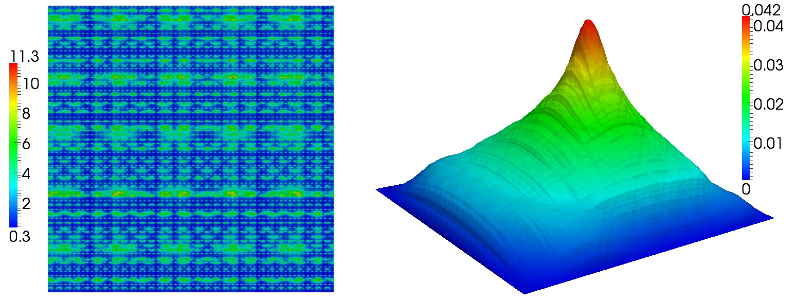
Figure 1: Model Problem 1. Left Picture: Plot of the coefficient $a^{\varepsilon}$ given by (72). Right Picture: reference solution $u_{h,\triangle t}$ at $t=1$ for $h=2^{-7}$.

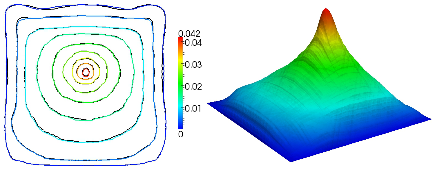
Figure 2: Model Problem 1, results for $t^{n}=1$. Left Picture: Comparison of the isolines of the reference solution $u_{h,\triangle t}$ for $h=2^{-7}$ (black isolines) with the multiscale approximation $u_{H,\triangle t,k}+Q_{h,k}(u_{H,\triangle t,k})$ for $(H,h,k)=(2^{-3},2^{-7},2)$ (colored isolines). Right Picture: Plot of the multiscale approximation $u_{H,\triangle t,k}+Q_{h,k}(u_{H,\triangle t,k})$ for $(H,h,k)=(2^{-3},2^{-7},2)$.

Table 1: Model Problem 1, results for $t^{n}=1$. The table depicts relative $L^{2}$- and $H^{1}$-errors for the obtained multiscale approximations with respect to the reference solution. The errors are defined in (70).

$H$	$k$	$\|e^{0,n}\|_{L^{2}(\Omega)}^{\mbox{\tiny rel}}$	$\|e^{\mbox{\rm\tiny ms},n}\|_{L^{2}(\Omega)}^{\mbox{\tiny rel}}$	$\|e^{\mbox{\rm\tiny ms},n}\|_{H^{1}(\Omega)}^{\mbox{\tiny rel}}$	$\|\partial_{t}e^{\mbox{\rm\tiny ms},n}\|_{L^{2}(\Omega)}^{\mbox{\tiny rel}}$	$\|\partial_{t}e^{\mbox{\rm\tiny ms},n}\|_{H^{1}(\Omega)}^{\mbox{\tiny rel}}$
$2^{-1}$	1	0.1448	0.1341	0.4532	0.8718	0.9957
$2^{-1}$	2	0.1394	0.1334	0.4627	0.8312	0.9822
$2^{-2}$	1	0.0780	0.0688	0.3517	0.6464	0.9424
$2^{-2}$	2	0.0687	0.0521	0.2919	0.5439	0.8949
$2^{-2}$	3	0.0675	0.0499	0.2835	0.5362	0.8929
$2^{-3}$	1	0.0368	0.0328	0.2279	0.5824	1.1262
$2^{-3}$	2	0.0242	0.0130	0.1212	0.3285	0.7769
$2^{-3}$	3	0.0234	0.0105	0.1036	0.2846	0.6998

Table 2: Model Problem 1, results for $t^{n}=1$. Overview on the EOCs associated with errors from Table 1. We couple $k$ and $H$ by $k=k(H):=\lfloor|\ln(H)|+1\rfloor$. For each of the errors $\|e_{H}\|$ below (for $H=2^{-i}$), we define the average EOC by EOC$:=\frac{1}{2}\sum_{i=1}^{2}\log_{2}(\|e_{2^{-i}}\|/\|e_{2^{-(i+1)}}\|)/\log_{2}(2)$.

$H$	$k(H)$	$\|e^{0,n}\|_{L^{2}(\Omega)}^{\mbox{\tiny rel}}$	$\|e^{\mbox{\rm\tiny ms},n}\|_{L^{2}(\Omega)}^{\mbox{\tiny rel}}$	$\|e^{\mbox{\rm\tiny ms},n}\|_{H^{1}(\Omega)}^{\mbox{\tiny rel}}$	$\|\partial_{t}e^{\mbox{\rm\tiny ms},n}\|_{L^{2}(\Omega)}^{\mbox{\tiny rel}}$	$\|\partial_{t}e^{\mbox{\rm\tiny ms},n}\|_{H^{1}(\Omega)}^{\mbox{\tiny rel}}$
$2^{-1}$	1	0.1448	0.1341	0.4532	0.8718	0.9957
$2^{-2}$	2	0.0687	0.0521	0.2919	0.5439	0.8949
$2^{-3}$	3	0.0234	0.0105	0.1036	0.2846	0.6998
EOC		1.31	1.84	1.06	0.81	0.25

In Table 1 the relative errors are depicted for various combinations of $H$ and $k$ (recall that $k$ denotes the truncation parameter defined in (12)). The errors are qualitatively comparable to the errors obtained in [33] for similar computations. Furthermore, we observe that the error evolution is consistent with the theoretically predicated rates. EOCs are given in Table 2.

For $k\approx|\ln(H)|+1$, we observe roughly a convergence rate of $1.3$ in $H$ for the $L^{2}$-error of the numerically homogenized solution $u_{H,\triangle t,k}$. Adding the corresponding corrector $Q_{h,k}(u_{H,\triangle t,k})$, the rate is close to $2$ in average. In Figure 2, a visual comparison between the reference solution and the multiscale approximation is shown. We observe that for $(H,h,k)=(2^{-3},2^{-7},2)$, the solution $u_{H,\triangle t,k}+Q_{h,k}(u_{H,\triangle t,k})$ looks the same as the reference solution $u_{h,\triangle t}$ depicted in (1). This is also stressed by the comparison of isolines in Figure 2.

6.2 Model problem 2

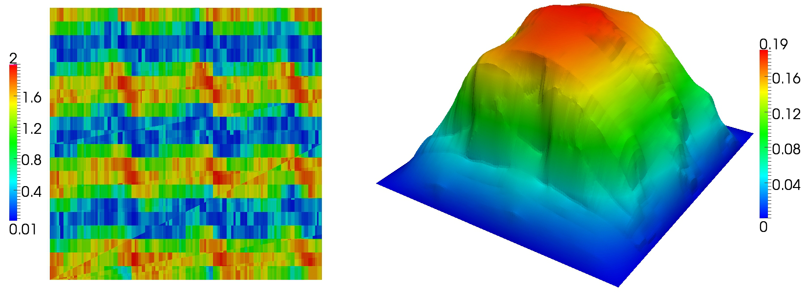
Figure 3: Model Problem 2, plots for $t^{n}=1$. Left Picture: Plot of the coefficient $a^{\varepsilon}$ given by (74). Right Picture: reference solution $u_{h,\triangle t}$ at $t=1$ for $h=2^{-8}$.

In Model Problem 2 we investigate the influence of a discontinuous coefficient $a^{\varepsilon}$ in our multiscale method. According to the theoretical results, it should not influence the convergence rates. The fine grid $\mathcal{T}_{h}$ is a uniformly refined triangulation with resolution $h=2^{-8}$.

Problem 6.2.

Let $\Omega:=]0,1[^{2}$ and $T:=1$. Find $u^{\varepsilon}\in L^{\infty}(0,T;H^{1}_{0}(\Omega))$ such that

$$\partial_{tt}u^{\varepsilon}(x,t)-\nabla\cdot\left(a^{\varepsilon}(x)\nabla u^{\varepsilon}(x,t)\right) =1\qquad\hskip 17.0pt\mbox{in }\Omega\times(0,T],$$

$$u^{\varepsilon}(x,t) =0\hskip 37.0pt\mbox{on }\partial\Omega\times[0,T],$$ (73)

$$u^{\varepsilon}(x,0)=0\quad\mbox{and}\quad\partial_{t}u^{\varepsilon}(x,0) =0\hskip 38.0pt\mbox{in }\Omega.$$

Here, we have

$$a^{\varepsilon}(x) :=(h\circ c_{\varepsilon})(x)\qquad\text{with}\enspace h(t):=\begin{cases}t^{4}&\text{for}\enspace\frac{1}{2}<t<1\\ t^{\frac{3}{2}}&\text{for}\enspace 1<t<\frac{3}{2}\\ t&\text{else}\end{cases}$$ (74)

and where

$$c_{\varepsilon}(x_{1},x_{2}):=1+\frac{1}{10}\sum_{j=0}^{4}\sum_{i=0}^{j}\left(\frac{2}{j+1}\cos\left(\bigl{\lfloor}ix_{2}-\tfrac{x_{1}}{1+i}\bigr{\rfloor}+\left\lfloor\tfrac{ix_{1}}{\varepsilon}\right\rfloor+\left\lfloor\tfrac{x_{2}}{\varepsilon}\right\rfloor\right)\right).$$

The coefficient $a^{\varepsilon}$ is plotted in Figure 3 together with the reference solution on $\mathcal{T}_{h}$ for $t=1$.

Table 3: Model Problem 2. Overview on relative $L^{2}$- and $H^{1}$-errors for Model Problem 2 for $t^{n}=1$. The errors are defined in (70).

$H$	$k$	$\|e^{0,n}\|_{L^{2}(\Omega)}^{\mbox{\tiny rel}}$	$\|e^{\mbox{\rm\tiny ms},n}\|_{L^{2}(\Omega)}^{\mbox{\tiny rel}}$	$\|e^{\mbox{\rm\tiny ms},n}\|_{H^{1}(\Omega)}^{\mbox{\tiny rel}}$	$\|\partial_{t}e^{\mbox{\rm\tiny ms},n}\|_{L^{2}(\Omega)}^{\mbox{\tiny rel}}$	$\|\partial_{t}e^{\mbox{\rm\tiny ms},n}\|_{H^{1}(\Omega)}^{\mbox{\tiny rel}}$
$2^{-2}$	1	0.1299	0.0613	0.1802	0.1762	0.6615
$2^{-2}$	2	0.1223	0.0245	0.0800	0.1298	0.6323
$2^{-3}$	1	0.0914	0.0616	0.1926	0.2194	0.7255
$2^{-3}$	2	0.0753	0.0191	0.0841	0.1049	0.5902
$2^{-3}$	3	0.0741	0.0085	0.0563	0.0870	0.5688
$2^{-4}$	1	0.0327	0.0243	0.1401	0.1197	0.6710
$2^{-4}$	2	0.0240	0.0047	0.0505	0.0600	0.5109
$2^{-4}$	3	0.0239	0.0029	0.0347	0.0562	0.5004

Table 4: Model Problem 2, results for $t^{n}=1$. Overview on the EOCs associated with errors from Table 3. We couple $k$ and $H$ by $k=k(H):=\lfloor|\ln(H)|+0.5\rfloor$. The average EOCs are computed according to (75).

$H$	$k(H)$	$\|e^{0,n}\|_{L^{2}(\Omega)}^{\mbox{\tiny rel}}$	$\|e^{\mbox{\rm\tiny ms},n}\|_{L^{2}(\Omega)}^{\mbox{\tiny rel}}$	$\|e^{\mbox{\rm\tiny ms},n}\|_{H^{1}(\Omega)}^{\mbox{\tiny rel}}$	$\|\partial_{t}e^{\mbox{\rm\tiny ms},n}\|_{L^{2}(\Omega)}^{\mbox{\tiny rel}}$	$\|\partial_{t}e^{\mbox{\rm\tiny ms},n}\|_{H^{1}(\Omega)}^{\mbox{\tiny rel}}$
$2^{-2}$	1	0.1299	0.0613	0.1802	0.1762	0.6615
$2^{-3}$	2	0.0753	0.0191	0.0841	0.1049	0.5902
$2^{-4}$	3	0.0239	0.0029	0.0347	0.0562	0.5004
EOC		1.22	2.20	1.19	0.82	0.20

In Table 3 we depict various relative $L^{2}$- and $H^{1}$-errors for $t^{n}=1$. We observe that the numerically homogenized solution $u_{H,\triangle t,k}$ already yields good $L^{2}$-approximation properties with respect to the fine scale reference solution. These approximation properties can still be significantly improved by adding the corrector $Q_{h,k}(u_{H,\triangle t,k})$. We can see that the total approximation $u_{H,\triangle t,k}+Q_{h,k}(u_{H,\triangle t,k})$ is also accurate in the norms $\|\nabla\cdot\|_{L^{2}(\Omega)}$ and $\|\partial_{t}\cdot\|_{L^{2}(\Omega)}$. The errors in the norm $\|\partial_{t}\cdot\|_{H^{1}(\Omega)}$ are noticeably larger than the errors in all other norms. Hence, the multiscale solution does not necessarily yield a highly accurate $H^{1}(0,T,H^{1}(\Omega))$ approximation, even though the discrepancy is still tolerable.

All errors for Model Problem 2 are of the same order as the errors for Model Problem 1 depicted in Table 1. In particular, we do not see any error deterioration caused by the discontinuity of the coefficient $a^{\varepsilon}$. The method behaves nicely in both cases. This is stressed by the experimental orders of convergence (EOCs) shown in Table 4. For the EOCs in Table 4, we use the average

$$\mbox{EOC}:=(\mbox{EOC}_{2^{-2}}+\mbox{EOC}_{2^{-3}})/2.$$ (75)

Motivated by Theorem 4.8, we couple the coarse mesh $H$ and the truncation parameter $k$ to be the closest integer to $|\ln(H)|$, i.e. we pick $k=k(H):=\lfloor|\ln(H)|+0.5\rfloor$ for the computation of the EOCs. This gives us $k=1$ for $H=2^{-2}$, $k=2$ for $H=2^{-3}$ and $k=3$ for $H=2^{-4}$. The corresponding results are stated in Table 4. We observe a close to linear convergence for the $L^{2}$-error for the numerically homogenized solution $u_{H,\triangle t,k}$ (as predicted by the theory). Adding the corrector $Q_{h,k}(u_{H,\triangle t,k})$, the convergence rate increases to $2.2$ (slightly worse than the optimal rate of $3$). For the $H^{1}$-error, we observe linear convergence. The convergence rate of the $L^{2}$-error for time derivatives is slightly below linear convergence, but still very satisfying. Only the convergence rate for the $H^{1}$-error for the time derivatives is close to stagnation.

Note that the deviation of these rates from the perfect rates comes from that fact that we do not know the generic constant $C_{\theta}$ in Theorem 4.8. We picked $k=|\ln(H)|$, instead of $k=C_{\theta}|\ln(H)|$. Still we observe that approximating $C_{\theta}$ by $1$ yields highly accurate results that are close to the optimal rates. Practically, this justifies the use of small localization patches $U_{k}(K)$.

6.3 Model problem 3

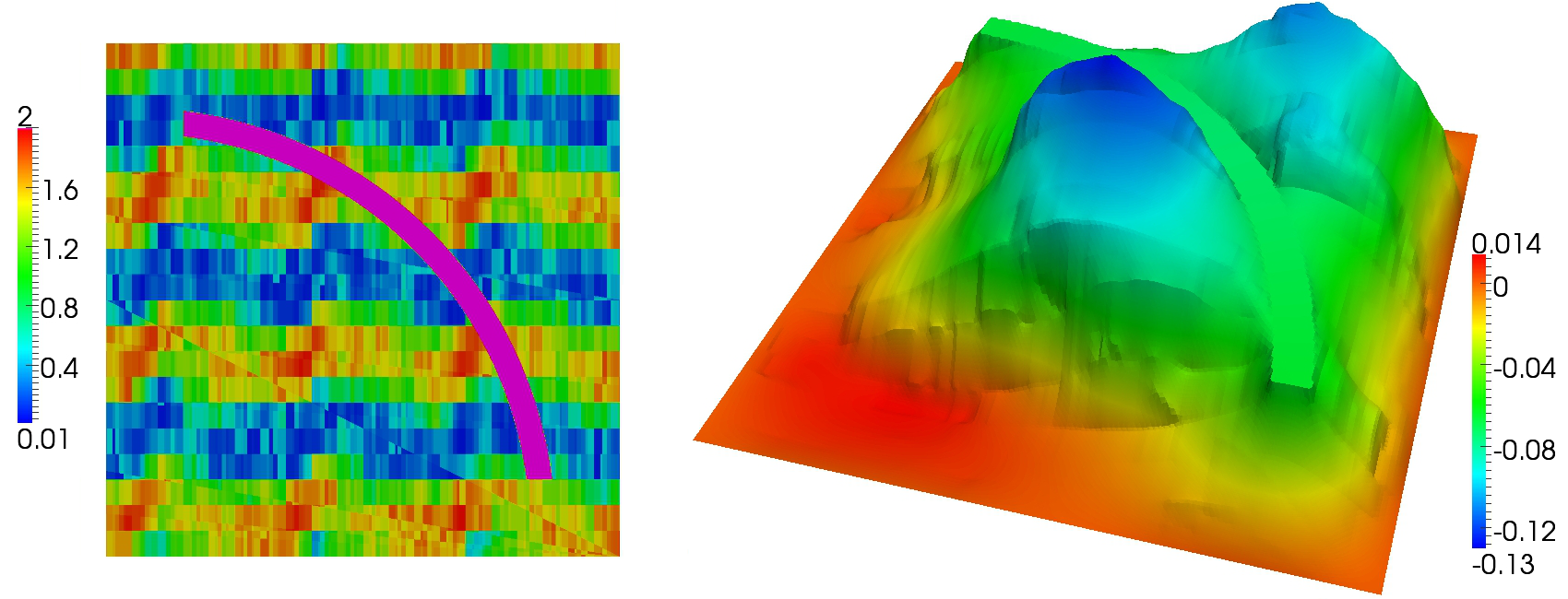
Figure 4: Model Problem 3. Left Picture: Plot of the coefficient $a^{\varepsilon}$. The basis structure of $a^{\varepsilon}$ is given by (74), but this structure is perturbed by an arc-like conductivity channel (pink). In this arc $a^{\varepsilon}$ takes the value $100$. Right Picture: reference solution $u_{h,\triangle t}$ at $t=1$ for $h=2^{-8}$.

Problem 6.3.

Let $\Omega:=]0,1[^{2}$ and $T:=1$. Find $u^{\varepsilon}\in L^{\infty}(0,T;H^{1}_{0}(\Omega))$ such that

$$\partial_{tt}u^{\varepsilon}(x,t)-\nabla\cdot\left(a^{\varepsilon}(x)\nabla u^{\varepsilon}(x,t)\right) =F(x,t)\qquad\hskip 17.0pt\mbox{in }\Omega\times(0,T],$$

$$u^{\varepsilon}(x,t) =0\hskip 66.0pt\mbox{on }\partial\Omega\times[0,T],$$ (76)

$$u^{\varepsilon}(x,0)=0\quad\mbox{and}\quad\partial_{t}u^{\varepsilon}(x,0) =0\hskip 66.0pt\mbox{in }\Omega.$$

Here, we have $F(x_{1},x_{2},t)=\sin(2.4x_{1}-1.8x_{2}+2\pi t)$ and $a^{\varepsilon}$ is given by equation (74) but additionally it is disturbed by a high conductivity channel of thickness 0.05. The precise structure of $a^{\varepsilon}$ is depicted in Figure 4, together with the reference solution on $\mathcal{T}_{h}$ for $t=1$.

Table 5: Model Problem 3, results for $t^{n}=1$. Overview on relative $L^{2}$- and $H^{1}$-errors defined as in (70).

$H$	$k$	$\|e^{0,n}\|_{L^{2}(\Omega)}^{\mbox{\tiny rel}}$	$\|e^{\mbox{\rm\tiny ms},n}\|_{L^{2}(\Omega)}^{\mbox{\tiny rel}}$	$\|e^{\mbox{\rm\tiny ms},n}\|_{H^{1}(\Omega)}^{\mbox{\tiny rel}}$	$\|\partial_{t}e^{\mbox{\rm\tiny ms},n}\|_{L^{2}(\Omega)}^{\mbox{\tiny rel}}$	$\|\partial_{t}e^{\mbox{\rm\tiny ms},n}\|_{H^{1}(\Omega)}^{\mbox{\tiny rel}}$
$2^{-2}$	1	0.2468	0.1564	0.3321	0.2066	0.4486
$2^{-2}$	2	0.2270	0.0782	0.1992	0.1168	0.3269
$2^{-3}$	1	0.1451	0.1046	0.3305	0.1639	0.4588
$2^{-3}$	2	0.1184	0.0329	0.1535	0.0607	0.2724
$2^{-3}$	3	0.1174	0.0202	0.1024	0.0468	0.2333
$2^{-4}$	1	0.0550	0.0433	0.2186	0.0667	0.3349
$2^{-4}$	2	0.0390	0.0095	0.0803	0.0250	0.1896
$2^{-4}$	3	0.0385	0.0046	0.0464	0.0198	0.1758

Table 6: Model Problem 3, results for $t^{n}=1$. Overview on the EOCs associated with errors from Table 5. We couple $k$ and $H$ by $k=k(H):=\lfloor|\ln(H)|+0.5\rfloor$. The average EOCs are computed according to (75).

$H$	$k(H)$	$\|e^{0,n}\|_{L^{2}(\Omega)}^{\mbox{\tiny rel}}$	$\|e^{\mbox{\rm\tiny ms},n}\|_{L^{2}(\Omega)}^{\mbox{\tiny rel}}$	$\|e^{\mbox{\rm\tiny ms},n}\|_{H^{1}(\Omega)}^{\mbox{\tiny rel}}$	$\|\partial_{t}e^{\mbox{\rm\tiny ms},n}\|_{L^{2}(\Omega)}^{\mbox{\tiny rel}}$	$\|\partial_{t}e^{\mbox{\rm\tiny ms},n}\|_{H^{1}(\Omega)}^{\mbox{\tiny rel}}$
$2^{-2}$	1	0.2468	0.1564	0.3321	0.2066	0.4486
$2^{-3}$	2	0.1184	0.0329	0.1535	0.0607	0.2724
$2^{-4}$	3	0.0385	0.0046	0.0464	0.0198	0.1758
EOC		1.34	2.54	1.42	1.69	0.68

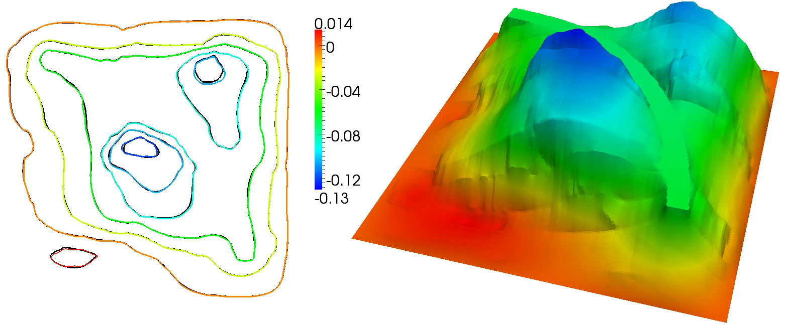
Figure 5: Model Problem 3, results at $t=1$. Left Picture: Comparison of the isolines of the reference solution $u_{h,\triangle t}$ for $h=2^{-8}$ (black isolines) with the multiscale approximation $u_{H,\triangle t,k}+Q_{h,k}(u_{H,\triangle t,k})$ for $(H,h,k)=(2^{-4},2^{-8},2)$ (colored isolines). Right Picture: Plot of the multiscale approximation $u_{H,\triangle t,k}+Q_{h,k}(u_{H,\triangle t,k})$ for $(H,h,k)=(2^{-4},2^{-8},2)$.

This model problem is inspired by a model problem in [33]. The source term as in [33] is given by $F(x_{1},x_{2},t)=\sin(2.4x_{1}-1.8x_{2}+2\pi t)$ and as in [33] $a^{\varepsilon}$ contains a conductivity channel that perturbs the original structure. As we could not access the data for the channel given in this reference we model a new one in this paper. This model problem is set to investigate the approximation quality of our multiscale approximations for problems with channels (which do not have to be resolved by the coarse grid) and a high contrast $\beta/\alpha\approx 10^{4}$. As in the previous model problem, we chose $\mathcal{T}_{h}$ as a uniformly refined triangulation with resolution $h=2^{-8}$.

We see in Table 5 that the additional channel in the problem does not deteriorate the convergence rates compared to Model Problem 2. Again, close to optimal convergence rates are obtained for the choice $k=k(H):=\lfloor|\ln(H)|+0.5\rfloor$ (which slightly underestimates the optimal truncation parameter $k$). The corresponding results are given in Table 5. The method yields accurate results even in the case of a conductivity channel and despite that the coarse grid does not resolve the channel. Furthermore the high contrast of order $10^{4}$ does not significantly influence the size of the optimal truncation parameter $k$. In the model problem we can still work with small localization patches $U_{k}(K)$, independent of the conductivity channel. This is further stressed by Figure 5 which depicts the multiscale approximation (i.e. $u_{H,\triangle t,k}+Q_{h,k}(u_{H,\triangle t,k})$) for the case $(H,k)=(2^{-4},2)$. The solution looks almost identical to the reference solution $u_{h,\triangle t}$ and the corresponding isolines match almost perfectly.

6.4 Model problem 4

In this model problem we investigate the performance of the multiscale method in the case of smooth, but not well-prepared initial values. In the light of Theorem 4.3, we can only expect a linear convergence rate with respect to $H$ and in the $L^{\infty}(L^{2})$-norm and we cannot expect any rates in the $W^{1,\infty}(L^{2})$- and $L^{\infty}(L^{2})$-norms, since Theorem 4.7 is not valid under general assumptions. As a model problem, we consider the setting of Model Problem 2, but with different source and initial values. As in the previous model problem, we chose $\mathcal{T}_{h}$ as a uniformly refined triangulation with resolution $h=2^{-8}$. We consider the following problem.

Problem 6.4.

Let $\Omega:=]0,1[^{2}$ and $T:=1$. Find $u^{\varepsilon}\in L^{\infty}(0,T;H^{1}_{0}(\Omega))$ such that

$$\partial_{tt}u^{\varepsilon}(x,t)-\nabla\cdot\left(a^{\varepsilon}(x)\nabla u^{\varepsilon}(x,t)\right) =F(x,t)\qquad\hskip 17.0pt\mbox{in }\Omega\times(0,T],$$

$$u^{\varepsilon}(x,t) =0\hskip 66.0pt\mbox{on }\partial\Omega\times[0,T],$$ (77)

$$u^{\varepsilon}(x,0)=f\quad\mbox{and}\quad\partial_{t}u^{\varepsilon}(x,0) =g\hskip 66.0pt\mbox{in }\Omega.$$

Here, we have $F(x_{1},x_{2})=\sin(2\pi x_{1})\sin(2\pi x_{2})$, $f(x_{1},x_{2})=x_{1}(1-x_{1})x_{2}(1-x_{2})$, $g(x_{1},x_{2})=\sin(2\pi x_{1})x_{2}(1-x_{2})$ and $a^{\varepsilon}$ is given by equation (74).

Table 7: Model Problem 4, results for $t^{n}=1$. Overview on relative $L^{2}$- and $H^{1}$-errors defined as in (70).

$H$	$k$	$\|e^{0,n}\|_{L^{2}(\Omega)}^{\mbox{\tiny rel}}$	$\|e^{\mbox{\rm\tiny ms},n}\|_{L^{2}(\Omega)}^{\mbox{\tiny rel}}$	$\|e^{\mbox{\rm\tiny ms},n}\|_{H^{1}(\Omega)}^{\mbox{\tiny rel}}$	$\|\partial_{t}e^{\mbox{\rm\tiny ms},n}\|_{L^{2}(\Omega)}^{\mbox{\tiny rel}}$	$\|\partial_{t}e^{\mbox{\rm\tiny ms},n}\|_{H^{1}(\Omega)}^{\mbox{\tiny rel}}$
$2^{-2}$	1	0.2809	0.2598	0.6180	0.3522	0.9735
$2^{-2}$	2	0.1865	0.1229	0.4954	0.3147	0.9692
$2^{-3}$	1	0.1579	0.1420	0.5680	0.3243	0.9691
$2^{-3}$	2	0.1188	0.0894	0.4869	0.2473	0.9593
$2^{-3}$	3	0.1145	0.0820	0.4741	0.2372	0.9573
$2^{-4}$	1	0.0885	0.0857	0.4774	0.2891	0.9850
$2^{-4}$	2	0.0466	0.0361	0.3249	0.1925	0.9506
$2^{-4}$	3	0.0423	0.0289	0.3042	0.1823	0.9479
$2^{-5}$	1	0.0499	0.0489	0.3481	0.1849	0.9593
$2^{-5}$	2	0.0198	0.0149	0.2256	0.1277	0.9204
$2^{-5}$	3	0.0173	0.0109	0.2059	0.1229	0.9171

Table 8: Model Problem 4, results for $t^{n}=1$. Overview on the EOCs associated with errors from Table 7. We couple $k$ and $H$ by $k=k(H):=\lfloor|\ln(H)|+0.5\rfloor$. The average EOCs are computed with $\mbox{EOC}:=(\mbox{EOC}_{2^{-2}}+\mbox{EOC}_{2^{-3}}+\mbox{EOC}_{2^{-4}})/3$.

$H$	$k(H)$	$\|e^{0,n}\|_{L^{2}(\Omega)}^{\mbox{\tiny rel}}$	$\|e^{\mbox{\rm\tiny ms},n}\|_{L^{2}(\Omega)}^{\mbox{\tiny rel}}$	$\|e^{\mbox{\rm\tiny ms},n}\|_{H^{1}(\Omega)}^{\mbox{\tiny rel}}$	$\|\partial_{t}e^{\mbox{\rm\tiny ms},n}\|_{L^{2}(\Omega)}^{\mbox{\tiny rel}}$	$\|\partial_{t}e^{\mbox{\rm\tiny ms},n}\|_{H^{1}(\Omega)}^{\mbox{\tiny rel}}$
$2^{-2}$	1	0.2809	0.2598	0.6180	0.3522	0.9735
$2^{-3}$	2	0.1188	0.0894	0.4869	0.2473	0.9593
$2^{-4}$	3	0.0423	0.0289	0.3042	0.1823	0.9479
$2^{-5}$	3	0.0173	0.0109	0.2059	0.1229	0.9171
EOC		1.34	1.53	0.53	0.51	0.03

The corresponding numerical results are depicted in Table 7. In order to compute the experimental orders of convergence, we pick as before the relation $k=k(H):=\lfloor|\ln(H)|+0.5\rfloor$ to compute a suitable truncation parameter. The results are shown in Table 8. The crucial observation that we make is that Theorem 4.3 seems to be indeed optimal and that Theorem 4.7 does not generalize to not well-prepared initial values. We observe that the $L^{\infty}(L^{2})$-error converges with an order between $1$ and $1.5$, which is just what we predicted. We also note that even though the error becomes slightly smaller when we use the corrector $Q_{h,k}(u_{H,k})$, the rates of convergence remain basically the same (this is in contrast to the case of well-prepared data, where we could improve the rates with the corrector). For the convergence rates for the error in the $W^{1,\infty}(L^{2})$- and $L^{\infty}(L^{2})$-norms we still observe a rate of order $0.5$, which might be an indication that a relaxed version of Theorem 4.7 might still hold for arbitrary initial values. However, from the analytical point a corresponding argument is still missing. The main conclusion that we can draw from Model Problem 4 is that we can also numerically confirm that the proposed multiscale method still works in the general setting of not well-prepared data. This is a significant observation that distinguishes our multiscale method from other multiscale methods for the wave equation.

Acknowledgements. This work is partially supported by the Swiss National Foundation, Grant: No $200021\_134716/1$ and by the Deutsche Forschungsgemeinschaft, DFG-Grant: OH 98/6-1. We would also like to thank the anonymous reviewers for their constructive feedback that helped us to improve the contents of this paper.

References

- [1] A. Abdulle. On a priori error analysis of fully discrete heterogeneous multiscale FEM. Multiscale Model. Simul., 4(2):447–459, 2005.
- [2] A. Abdulle. Analysis of a heterogeneous multiscale FEM for problems in elasticity. Math. Models Methods Appl. Sci., 16(4):615–635, 2006.
- [3] A. Abdulle. A priori and a posteriori error analysis for numerical homogenization: a unified framework. Ser. Contemp. Appl. Math. CAM, 16:280–305, 2011.
- [4] A. Abdulle and M. J. Grote. Finite element heterogeneous multiscale method for the wave equation. Multiscale Model. Simul., 9(2):766–792, 2011.
- [5] A. Abdulle, M. J. Grote, and C. Stohrer. FE heterogeneous multiscale method for long-time wave propagation. C. R. Math. Acad. Sci. Paris, 351(11-12):495–499, 2013.
- [6] A. Abdulle, M. J. Grote, and C. Stohrer. Finite element heterogeneous multiscale method for the wave equation: long-time effects. Multiscale Model. Simul., 12(3):1230–1257, 2014.
- [7] G. Allaire and R. Orive. Homogenization of periodic non self-adjoint problems with large drift and potential. ESAIM Control Optim. Calc. Var., 13(4):735–749 (electronic), 2007.
- [8] G. A. Baker. Error estimates for finite element methods for second order hyperbolic equations. SIAM J. Numer. Anal., 13(4):564–576, 1976.
- [9] R. E. Bank and T. Dupont. An optimal order process for solving finite element equations. Math. Comp., 36(153):35–51, 1981.
- [10] R. E. Bank and H. Yserentant. On the -stability of the -projection onto finite element spaces. Numer. Math., 126(2):361–381, 2014.
- [11] S. Brahim-Otsmane, G. A. Francfort, and F. Murat. Correctors for the homogenization of the wave and heat equations. J. Math. Pures Appl., 71(3):197–231, 1992.
- [12] C. Carstensen. Quasi-interpolation and a posteriori error analysis in finite element methods. M2AN Math. Model. Numer. Anal., 33(6):1187–1202, 1999.
- [13] D. Cioranescu and P. Donato. An introduction to homogenization, volume 17 of Oxford Lecture Series in Mathematics and its Applications. Oxford University Press, New York, 1999.
- [14] W. E and B. Engquist. The heterogeneous multiscale methods. Commun. Math. Sci., 1(1):87–132, 2003.
- [15] D. Elfverson, E. H. Georgoulis, A. Målqvist, and D. Peterseim. Convergence of a discontinuous Galerkin multiscale method. SIAM J. Numer. Anal., 51(6):3351–3372, 2013.
- [16] B. Engquist, H. Holst, and O. Runborg. Multi-scale methods for wave propagation in heterogeneous media. Commun. Math. Sci., 9(1), 2011.
- [17] B. Engquist, H. Holst, and O. Runborg. Multiscale methods for wave propagation in heterogeneous media over long time. In Numerical analysis of multiscale computations, pages 167–186. Springer, 2012.
- [18] L. C. Evans. Partial differential equations, volume 19 of Graduate Studies in Mathematics. American Mathematical Society, Providence, RI, second edition, 2010.
- [19] P. Henning and A. Målqvist. Localized orthogonal decomposition techniques for boundary value problems. SIAM J. Sci. Comput., 36(4):A1609–A1634, 2014.
- [20] P. Henning, A. Målqvist, and D. Peterseim. A localized orthogonal decomposition method for semi-linear elliptic problems. M2AN Math. Model. Numer. Anal., 48(5):1331–1349, 2014.
- [21] P. Henning and M. Ohlberger. The heterogeneous multiscale finite element method for elliptic homogenization problems in perforated domains. Numer. Math., 113(4):601–629, 2009.
- [22] P. Henning and D. Peterseim. Oversampling for the Multiscale Finite Element Method. SIAM Multiscale Model. Simul., 11(4):1149–1175, 2013.
- [23] T. J. R. Hughes, G. R. Feijóo, L. Mazzei, and J.-B. Quincy. The variational multiscale method—a paradigm for computational mechanics. Comput. Methods Appl. Mech. Engrg., 166(1-2):3–24, 1998.
- [24] L. Jiang and Y. Efendiev. A priori estimates for two multiscale finite element methods using multiple global fields to wave equations. Numer. Methods Partial Differential Equations, 28(6):1869–1892, 2012.
- [25] L. Jiang, Y. Efendiev, and V. Ginting. Analysis of global multiscale finite element methods for wave equations with continuum spatial scales. Appl. Numer. Math., 60(8):862–876, 2010.
- [26] O. Korostyshevskaya and S. E. Minkoff. A matrix analysis of operator-based upscaling for the wave equation. SIAM J. Numer. Anal., 44(2):586–612 (electronic), 2006.
- [27] A. Lamacz. Dispersive effective models for waves in heterogeneous media. Math. Models Methods Appl. Sci., 21(9):1871–1899, 2011.
- [28] M. G. Larson and A. Målqvist. Adaptive variational multiscale methods based on a posteriori error estimation: energy norm estimates for elliptic problems. Comput. Methods Appl. Mech. Engrg., 196(21-24):2313–2324, 2007.
- [29] J.-L. Lions and E. Magenes. Non-homogeneous boundary value problems and applications. Vol. I. Springer-Verlag, New York, 1972. Translated from the French by P. Kenneth, Die Grundlehren der mathematischen Wissenschaften, Band 181.
- [30] A. Målqvist. Multiscale methods for elliptic problems. Multiscale Model. Simul., 9(3):1064–1086, 2011.
- [31] A. Målqvist and D. Peterseim. Localization of elliptic multiscale problems. Math. Comp., 83(290):2583–2603, 2014.
- [32] A. Målqvist and D. Peterseim. Computation of eigenvalues by numerical upscaling. Numer. Math., 130(2):337–361, 2015.
- [33] H. Owhadi and L. Zhang. Numerical homogenization of the acoustic wave equations with a continuum of scales. Comput. Methods Appl. Mech. Engrg., 198(3):397–406, 2008.
- [34] H. Owhadi and L. Zhang. Localized bases for finite-dimensional homogenization approximations with nonseparated scales and high contrast. Multiscale Model. Simul., 9(4):1373–1398, 2011.
- [35] S. Spagnolo. Sulla convergenza di soluzioni di equazioni paraboliche ed ellittiche. Ann. Sc. Norm. Super. Pisa Cl. Sci., 22(4):571–597, 1968.
- [36] L. Tartar. Cours Peccot. Collège de France, 1977.
- [37] T. Vdovina, S. E. Minkoff, and O. Korostyshevskaya. Operator upscaling for the acoustic wave equation. Multiscale Model. Simul., 4(4):1305–1338 (electronic), 2005.