Spectral classes of regular, random, and empirical graphs

Abstract

We define a (pseudo-)distance between graphs based on the spectrum of the normalized Laplacian, which is easy to compute or to estimate numerically. It can therefore serve as a rough classification of large empirical graphs into families that share the same asymptotic behavior of the spectrum so that the distance of two graphs from the same family is bounded by $\mathcal{O}(1/n)$ in terms of size $n$ of their vertex sets. Numerical experiments demonstrate that the spectral distance provides a practically useful measure of graph dissimilarity.

Keywords: Quasimetric; Laplacian spectrum; Radon measure; Graph families;

1 Introduction

Structural comparison of graphs has important applications in biology and pattern recognition, see e.g. [1, 2]. The problem comes in two distinct flavors: it is comparably easy when correspondences between nodes are known. This is the case e.g. for the comparison of metabolic networks or protein-protein interaction networks [3]. The problem becomes much more difficult when node correspondences are unknown, as is the case e.g. in the atom-mapping problem reviewed in [4]. A classical combinatorial formulation of the latter problem is to find the largest graph $G$ that is isomorphic to a subgraph of each of two given input graphs $G_{1}$ and $G_{2}$. A natural metric distance is given by $d_{MCSI}(G_{1},G_{2}):=\|G_{1}\setminus G\|+\|G_{2}\setminus G\|$, were $\|\cdot\|$ is measure of graph size, e.g. the sum of edges and vertices. The main difficulty for practical applications is that “maximum common subgraph isomorphism problem” is NP-complete [5, 6] and even APX-hard [7].

For large graphs, thus, more computationally efficient distance measures are required. Graph kernels [8] describe graphs as vectors of features, usually the occurrence data of small subgraphs have increasingly been used in bioinformatics [9] and chemoinformatics [10]. A related approach computed the earth movement distance between the distributions of graph features [11]. A practical difficulty is the fact that a very large number of features is required to achieve sufficient resolution for very large graphs.

Here we pursue a different approach that makes use of the representation of graphs by its adjacency or its Laplacian matrix. Spectral properties of these matrix representation are closely related to the graph structure [12, 13, 14]. Spectral graph theory in turn has received much inspiration from eigenvalue estimates in Riemannian geometry, see e.g. [12, 15, 16]. Many of these estimates involve only particular eigenvalues, like the smallest or largest. Here, instead we wish to compare the entire spectra of two graphs to get some idea of how similar or different they are [17]. The advantage of such an approach is that nowadays, there exist very efficient and numerically stable algorithms for computing the eigenvalues of a large $(N\times N)$-matrix, in fact with an effort of only $\mathcal{O}(N^{2})$ in practice [18]. For the set of graphs of the same size, a spectral distance based on the adjacency matrix was suggested in [19] as a cospectral measure and further studied in [20]. Although co-spectral graphs do exist, and it remains an open problem what fraction of graphs is uniquely determined by its spectrum [21], we shall see that the comparison of graph spectra nevertheless provides as sensitive and computationally attractive graph distance. We propose here a spectral distance associated with the normalized Laplacian instead of the adjacency matrix, without any constraint on the graph sizes. The reason is that the normalized Laplacian, with its natural random walk or diffusion interpretation, seems to capture some geometric properties better than the adjacency matrix.

Throughout this paper we assume that $G=(V,E)$ is a simple graph, i.e. a finite, undirected, unweighted graph without self-loops or multiple edges, where $V$ and $E$ are the vertex and edge sets. $n=|V|$ is the size of $G$. We denote adjacency of $x$ and $y$ interchangeably as $x\sim y$ or $xy\in E$.

The normalized Laplacian $\Delta_{G}$ of $G$ operates on functions $f:V\to{\mathbb{R}}$ by

$$\Delta_{G}f(x)=f(x)-\frac{1}{d_{x}}\sum_{y\sim x}f(y),$$ (1.1)

where $d_{x}$, the degree of $x$, is the number of edges connected to $x$. $\Delta_{G}$ is a bounded and self-adjoint operator. The definition of $\Delta$ can be expanded without difficulty to weighted graphs and with some more effort also to directed ones. We will not explicitly consider these more general cases here.

The spectrum of $\Delta_{G}$, denoted by $\lambda(G)$, consists of $n$ eigenvalues, all contained in $[0,2]$, i.e., $0=\lambda_{0}\leq\lambda_{1}\leq\ldots\leq\lambda_{n-1}\leq 2$. This yields the Radon probability measure

$$\mu(G)=\frac{1}{n}\sum_{i=0}^{n-1}\delta_{{\lambda}_{i}(G)}$$ (1.2)

on $[0,2]$, where $\delta_{\cdot}$ denotes the Dirac measure. We can then integrate functions against this measure, for instance a Gaussian kernel with center $x$ and bandwidth $\sigma$, to obtain [22, 23],

$$\rho_{G}(x)=\frac{1}{n}\sum\limits_{i=0}^{n-1}{\frac{1}{\sqrt{2\pi\sigma^{2}}}e^{-\frac{(x-\lambda_{i})^{2}}{2\sigma^{2}}}}.$$ (1.3)

$\rho_{G}$ thus is a smoothed spectral density of $G$. It naturally gives rise to a pseudometric on the space of simple graphs by means of the $\ell^{1}$ distance of the spectral densities:

$$D(G,G^{\prime}):=\int|\rho_{G}(x)-\rho_{G^{\prime}}(x)|dx.$$ (1.4)

Remark 1.1.

It is obvious that $D$ yields a pseudometric on the space of (isomorphism classes of) graphs. $D$ is not a distance because of the possibility of cospectral graphs, that is, non-isomorphic graphs with the same spectrum, see [18] for a survey. Nevertheless, we shall call $D(G,G^{\prime})$ the “spectral distance” between the graphs $G$ and $G^{\prime}$.

Remark 1.2.

The fact that all complete bipartite graphs $K_{n_{1},n_{2}}$ with the same total number $n=n_{1}+n_{2}$ of vertices have the same spectrum (it consists of 0 and 2 with multiplicity 1 and of 1 with multiplicity $n-2$) shows that the spectrum of the normalized Laplacian is not sensitive to the number of edges. This can be easily remedied, however, by using the (normalized) Laplacian on edges rather than on vertices. Then, see [24], the spectrum is the same as that for vertices, except for the multiplicity of the eigenvalue zero which now counts the number of independent cycles, that is, is equal to $|E|-|V|+1$. In contrast, for the Laplacian on vertices that we have used here, the multiplicity of the eigenvalue 0 is equal to the number of connected components. All subsequent constructions will work for the Laplacian on edges as for that on vertices.

In Section 2, the asymptotic behavior of families $G_{n}$ of finite graphs is discussed, when their number $n$ of vertices tends to infinity. It turns out that typical classes of graphs, like complete, complete bipartite, cycle, path, cube, have characteristic asymptotic properties of the corresponding measures $\mu$ from (1.2). In section 3, using the interlacing theory, we prove that the distance between two finite graphs of size of order $n$ that differ only in finitely many edit operations is equal to $\mathcal{O}(1/n)$. Moreover, we show that the distance for particular pairs of graphs converges to zero even with speed with $\mathcal{O}(1/n^{2})$ in many cases. Finally, in the numerical part of this paper, we compare spectral distances within families of random graphs.

2 Spectral classes of graphs

Empirical studies have shown that qualitatively different type of large graphs can in many cases be distinguished by the shape of their spectral density. For example, in 1955, Wigner introduced his famous semicircle law, which says that the spectrum of a large random symmetric matrix follows a semicircle distribution [25, 26, 27]. In [28], it was found that the spectral distribution is an important characteristic of a network, and a classification scheme for empirical networks based on the spectral plot of the Laplacian of the graph underlying the network was introduced.

Let $(G_{n})_{n\in\mathbb{N}}$ be an infinite family of graphs $G_{n}$ of $n$ vertices. An important recent development in graph theory is concerned with the construction of suitable limits of such families for $n\to\infty$. Typically, such limits should reflect the asymptotic distribution of isomorphism classes of subgraphs. For dense graphs, one obtains the graphons, whereas for sparse graphs, one has the notion of graphings, see Lovász’ monograph [29] for an overview. Here, we propose a weaker notion that is based on graph spectra, more precisely on the Radon measure defined in (1.2). Thus, for a continuous function $f:[0,2]\to{\mathbb{R}}$, we have

$$\mu(G)(f)=\frac{1}{n}\sum_{i=0}^{n-1}f({\lambda}_{i}(G)).$$ (2.1)

Recall that a family $\mu_{n}$ of Radon measures on $[0,2]$ converges weakly to the Radon measure $\mu_{0}$, in symbols $\mu_{n}\rightharpoondown\mu_{0}$, if $\mu_{0}(f)=\lim_{n\to\infty}\mu_{n}(f)$ for all continuous functions $f:[0,2]\to{\mathbb{R}}$.

Definition 2.1.

A family $(G_{n})_{n\in{\mathbb{N}}}$ of graphs belongs to the spectral class $\rho$, where $\rho$ is a Radon measure on $[0,2]$, if $\mu(G_{n})\rightharpoondown\rho$ for $n\to\infty$.

To demonstrate that this definition is meaningful, we consider a few simple examples.

Proposition 2.2.

Let $G_{n}=K_{n}$, the complete graph on $n$ vertices, or $G_{n}=K_{n_{1},n_{2}}$, the complete bipartite graph on $n_{1}+n_{2}=n$ vertices. Then $G_{n}$ belongs to the spectral class $\delta_{1}$, where $\delta_{1}$ is the Dirac measure supported at $1$.

In particular, the complete and the complete bipartite graphs asymptotically belong to the same spectral class.

Proof.

The spectrum of $K_{n}$ consists of $0$ with multiplicity 1 and of $\frac{n-1}{n}$ with multiplicity $n-1$, and that of $K_{n_{1},n_{2}}$ of $0$ and $2$ with multiplicity 1 each and $1$ with multiplicity $n-2$. This easily implies the result. ∎

In fact, the family of $n$-cubes also asymptotically belongs to the same spectral class.

Proposition 2.3.

Let $G_{n}$ be the $n$-cube on $2^{n}$ vertices, then the corresponding spectral class is given by $\delta_{1}$.

Proof.

The spectrum of the $n$-cube consists of $\frac{2k}{n}$ with multiplicity $\binom{n}{k}$, where $k=0,\ldots,n$. For any continuous function $f:[0,2]\rightarrow\mathbb{R}$, $\forall\varepsilon>0$, there exists a sufficiently small constant $\alpha\in(0,\frac{1}{2})$, such that $|f(x)-f(1)|<\varepsilon$ for any $x\in(1-2\alpha,1+2\alpha)$. Then,

$$\left|\lim_{n\to\infty}\sum\limits_{k=0}^{n}\frac{1}{2^{n}}\binom{n}{k}f\left(\frac{2k}{n}\right)-f(1)\right|$$

$$\leq \left|\lim_{n\to\infty}\sum\limits_{k=0}^{[\frac{n}{2}(1-\alpha)]-1}\frac{1}{2^{n}}\binom{n}{k}f\left(\frac{2k}{n}\right)\right|+\left|\lim_{n\to\infty}\sum\limits_{k=[\frac{n}{2}(1+\alpha)]+1}^{n}\frac{1}{2^{n}}\binom{n}{k}f\left(\frac{2k}{n}\right)\right|$$

$$+\left|\lim_{n\to\infty}\sum\limits_{k=[\frac{n}{2}(1-\alpha)]}^{[\frac{n}{2}(1+\alpha)]}\frac{1}{2^{n}}\binom{n}{k}f\left(\frac{2k}{n}\right)-f(1)\right|$$

$$\leq \max\limits_{x\in[0,2]}\left|f(x)\right|\lim_{n\to\infty}\sum\limits_{k=0}^{[\frac{n}{2}(1-\alpha)]-1}\frac{1}{2^{n}}\binom{n}{k}+\max\limits_{x\in[0,2]}\left|f(x)\right|\lim_{n\to\infty}\sum\limits_{k=[\frac{n}{2}(1+\alpha)]+1}^{n}\frac{1}{2^{n}}\binom{n}{k}$$

$$+\left|\lim_{n\to\infty}\sum\limits_{k=[\frac{n}{2}(1-\alpha)]}^{[\frac{n}{2}(1+\alpha)]}\frac{1}{2^{n}}\binom{n}{k}f\left(\frac{2k}{n}\right)-f(1)\right|.$$

With Stirling’s approximation $n!\thickapprox\sqrt{2\pi n}(\frac{n}{e})^{n}$ [30] and $t:=\frac{1-\alpha}{2}$, we obtain

$$\lim\limits_{n\to\infty}\sum\limits_{k=0}^{[\frac{n}{2}(1-\alpha)]-1}\frac{1}{2^{n}}\binom{n}{k}\leq\lim_{n\to\infty}\frac{nt}{2^{n}}\binom{n}{nt-1}\leq\lim_{n\to\infty}\frac{nt}{e^{n\log 2}}\binom{n}{nt}$$

$$= \lim_{n\to\infty}\frac{t\sqrt{n}}{\sqrt{2\pi}e^{n\log 2}}\frac{1}{e^{nt\log t+n(1-t)\log(1-t)+\frac{1}{2}\log t+\frac{1}{2}\log(1-t)}}$$

Suppose $g(s)=s\log s+(1-s)\log(1-s)$ for $s\in(0,1)$, then $g^{\prime}(s)=\log s-\log(1-s)$, we know $g(s)$ attains its minimal value $-\log 2$ at $\frac{1}{2}$. Then we have $g(\frac{1-\alpha}{2})=-\log 2+C_{\alpha}$ for some positive constant $C_{\alpha}$ depending on $\alpha$. Therefore, $\lim\limits_{n\to\infty}\sum\limits_{k=0}^{[\frac{n}{2}(1-\alpha)]-1}\frac{1}{2^{n}}\binom{n}{k}=0$. Similarity, we also can prove $\lim\limits_{n\to\infty}\sum\limits_{k=[\frac{n}{2}(1+\alpha)]+1}^{n}\frac{1}{2^{n}}\binom{n}{k}=0$. Combined with $\sum\limits_{k=0}^{n}\frac{1}{2^{n}}\binom{n}{k}=1$, we have,

$$\left|\lim_{n\to\infty}\sum\limits_{k=0}^{n}\frac{1}{2^{n}}\binom{n}{k}f(\frac{2k}{n})-f(1)\right|\leq\left|\lim_{n\to\infty}\sum\limits_{k=[\frac{n}{2}(1-\alpha)]}^{[\frac{n}{2}(1+\alpha)]}\frac{1}{2^{n}}\binom{n}{k}f(\frac{2k}{n})-f(1)\right|$$

$$\leq \left|\lim_{n\to\infty}\sum\limits_{k=[\frac{n}{2}(1-\alpha)]}^{[\frac{n}{2}(1+\alpha)]}\frac{1}{2^{n}}\binom{n}{k}\left(f(\frac{2k}{n})-f(1)\right)\right|$$

$$\leq \lim_{n\to\infty}\sum\limits_{k=[\frac{n}{2}(1-\alpha)]}^{[\frac{n}{2}(1+\alpha)]}\frac{1}{2^{n}}\binom{n}{k}\varepsilon\leq\varepsilon$$

So, we have

$$\lim_{n\to\infty}\sum\limits_{k=0}^{n}\frac{1}{2^{n}}\binom{n}{k}f(\frac{2k}{n})=f(1).$$

Hence, for $G_{n}$, the corresponding spectral class is $\delta_{1}$. ∎

Proposition 2.4.

Let $G_{n}$ be the petal graph on $n=2m+1$ vertices, that is, the graph consisting of $m$ triangles all joined at one vertex (this vertex then has degree $2m$, whereas all other vertices are of degree 2). The spectral class then is given by $\frac{1}{2}\delta_{\frac{1}{2}}+\frac{1}{2}\delta_{\frac{3}{2}}$.

Proof.

The spectrum of $G_{n}$ consists of $0$ with multiplicity 1, $\frac{1}{2}$ with multiplicity $m-1$ and $\frac{3}{2}$ with multiplicity $m+1$. ∎

Proposition 2.5.

In contrast, when $G_{n}=P_{n}$, the path with $n$ nodes, or $G_{n}=C_{n}$, the cycle with $n$ nodes, then the corresponding spectral class $\rho$ has no atoms, that is, $\rho(A)=0$ whenever $A$ is a finite subset of $[0,2]$, for instance a single point. In fact, $\rho$ is absolutely continuous with respect to the Lebesgue measure on $[0,2]$ with a probability density function (see Fig. 1)

$$g(x)=\frac{1}{\pi}\frac{1}{\sqrt{2x-x^{2}}}.$$ (2.2)

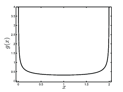
Figure 1: The probability density function $g(x)$.

Proof.

The spectrum of $P_{n}$ consists of $1-\cos\frac{\pi k}{n-1}$ with equal multiplicity 1, where $k=0,\ldots,n-1$. Denote the cumulative distribution functions of $\mu(P_{n})$ by $F_{n}(x):=\mu(P_{n})([0,x])$ for $0\leq x\leq 2$. We observe that

$$F_{n}(x)=\frac{1}{n}\left(\left[\frac{n-1}{\pi}\arccos(1-x)\right]+1\right)$$ (2.3)

and then

$$\lim_{n\rightarrow\infty}F_{n}(x)=\frac{1}{\pi}\arccos(1-x):=F(x).$$ (2.4)

Let $\rho$ be the probability measure such that $d\rho(x)=g(x)dx$, $x\in[0,2]$. Then $F$ is the cumulative distribution function of $\rho$. By the property of weak convergence of probability measures on $\mathbb{R}$, we know $\mu(P_{n})\rightharpoondown\rho$. The case for $C_{n}$ with the spectrum $1-\cos\frac{2\pi k}{n}$, where $k=0,\ldots,n-1$, can be proved similarly. They belong to the same spectral class $\rho$. ∎

There also exist families $(G_{n})$ whose asymptotic spectral contains both a Dirac and a regular component. For instance, take the graph $G_{n}$ with $n=3m$ obtained from an even cycle $C_{2m}$ where every other node is duplicated. According to [31], this graph has the eigenvalue $1$ with multiplicity $m$, but it also inherits a slightly perturbed version of the spectrum of $C_{2m}$. The latter yields a regular contribution to the asymptotic spectral measure, whereas the former contributes an atomic part $\frac{1}{3}\delta_{1}$.

Given an arbitrary family of graphs, the corresponding spectral class may be not well-defined.

Example 2.6.

Let $G_{n}$ be given as follows.

$$G_{n}=\left\{\begin{array}[]{ll}K_{n},&\hbox{if $n$ even;}\\ \text{petal graph},&\hbox{if $n$ odd.}\end{array}\right.$$

Then there is no well-defined spectral class for $(G_{n})_{n\in\mathbb{N}}$.

However, by the Prokhorov theorem [32], we know that for any family $(G_{n})$ of graphs, there at least exists a sub-family of it which belong to one spectral class.

The main result of this section is that two graph families that differ only by finite modifications do not differ in their asymptotic spectral class. Normally, two graphs could be related to each other through some modification. We define the following modification as the edit operations.

Definition 2.7.

An edit operation on a graph $G$ is the insertion or deletion of an edge or the insertion or deletion of an isolated vertex.

A finite graph always can be changed to another finite one through finitely many edit operations. If $G^{\prime}$ and $G^{\prime\prime}$ are connected there is always a sequence of edit operations so that all intermediates are also finite. Furthermore, one may “couple” the insertion and deletion of isolated vertices with the insertion of the first and the deletion of the last edges that it is incident with, so that graph editing can be specified in terms of edge insertions and edge deletions. The edit distance $d_{\textrm{edit}}(G^{\prime},G^{\prime\prime})$ between two graphs $G^{\prime}$ and $G^{\prime\prime}$ can be defined as the minimal number of edge operations required to convert $G^{\prime}$ into $G^{\prime\prime}$. It is well known that $d_{\textrm{edit}}$ is a metric and equals $|E(G^{\prime})|+|E(G^{\prime\prime})|-2|E(H)|$, where $H$ is the edge-maximal common subgraph of $G^{\prime}$ and $G^{\prime\prime}$, which is very hard to compute.

Theorem 2.8.

Let $G_{n}$ and $G^{\prime}_{n^{\prime}}$ be graphs with $n$ and $n^{\prime}$ vertices, respectively. Assume that $G^{\prime}_{n^{\prime}}$ can be obtained from $G_{n}$ by at most $C$ steps of edit operations, where $C$ is independent of $n$. Then the families $(G_{n})$ and $(G^{\prime}_{n^{\prime}})$ belong to the same spectral class (assuming that the corresponding spectral measures possess weak limits).

Theorem 2.8 is a consequence of the interlacing properties of the Lapacian spectra [33, 16, 34] for very similar graphs. More precisely, the eigenvalues of two graphs $G$ and $G^{\prime}$ control each other by virtue of inequalities of the form

$$\lambda_{i-t_{1}}\leq\lambda^{\prime}_{i}\leq\lambda_{i+t_{2}},$$ (2.5)

where the integers $t_{1}$ and $t_{2}$ are independent of the index $i$ but explicitly depend on the topological characteristics of the operation required to convert $G$ to $G^{\prime}$. Interlacing properties for the normalized Laplacian spectra were studied in particular in [34].

Lemma 2.9.

Let $G$ and $G^{\prime}$ be two graphs as in Theorem 2.8 and let $\lambda_{0}\leq\lambda_{1}\leq\cdots\leq\lambda_{n-1}$ and $\theta_{0}\leq\theta_{1}\leq\cdots\leq\theta_{n^{\prime}-1}$ be the eigenvalues of $\Delta_{G}$ and $\Delta_{G^{\prime}}$, respectively. We then have a constant $C$ so that

$$\lambda_{i-C}\leq\theta_{i}\leq\lambda_{i+C}$$ (2.6)

holds for $i=0,1,\ldots,n-1$, where we used the notations $\lambda_{j}=0$ for $j<0$ and $\lambda_{j}=2$ for $j\geq n$.

Proof.

Without loss of generality, we suppose $n^{\prime}\geq n$. Then we can obtain $G^{\prime}$ from $G$ by firstly adding $(n^{\prime}-n)$ isolated vertices, then deleting $t_{1}$ edges and finally adding $t_{2}$ edges. Note adding $(n^{\prime}-n)$ isolated vertices to $G^{\prime}$ produces $(n^{\prime}-n)$ additional zero eigenvalues. Set $C:=n^{\prime}-n+t_{1}+t_{2}$. Then (2.6) is a direct corollary of Theorem 2.3 in [34], where the interlacing inequalities for deleting one edge is proved. ∎

With the above lemma, we can prove Theorem 2.8.

Proof of Theorem 2.8.

Suppose $G$ and $G^{\prime}$ have normalized Laplacian spectra

$$0=\lambda_{0}\leq\lambda_{1}\leq\ldots\leq\lambda_{n-1}\leq 2\mbox{ and }0=\theta_{0}\leq\theta_{1}\leq\ldots\leq\theta_{n^{\prime}-1}\leq 2,$$

respectively. Without loss of generality, we suppose $n^{\prime}-n=C^{\prime}\leq C$. According to Lemma 2.9, we have

$$\lambda_{i-C}\leq\theta_{i}\leq\lambda_{i+C}.$$

Let $f:[0,2]\rightarrow\mathbb{R}$ be a continuous function. By approximation, we may assume that $f$ is differentiable. $f$ can be decomposed into the sum $f=\tilde{f_{+}}+\tilde{f_{-}}$ of a monotonically increasing function $\tilde{f_{+}}=\int_{0}^{x}(f^{\prime})^{+}+f(0)$ and a monotonically decreasing function $\tilde{f_{-}}=\int_{0}^{x}(f^{\prime})^{-}$. For continuous monotonic functions $F$ in $[0,2]$, we have,

$$\lim_{n\to\infty}{\left(\frac{1}{n}\sum\limits_{i=0}^{n-1}F(\lambda_{i})-\frac{1}{n}\sum\limits_{i=-C}^{n-C-1}F(\theta_{i})\right)}\geq 0$$

and

$$\lim_{n\to\infty}{\left(\frac{1}{n}\sum\limits_{i=0}^{n-1}F(\lambda_{i})-\frac{1}{n}\sum\limits_{i=C}^{n+C-1}F(\theta_{i})\right)}\leq 0.$$

Because $C^{\prime}\leq C$ is bounded and independent on $n$, and $F(x)$ is always bounded, we have,

$$\lim_{n\to\infty}{\left(\frac{1}{n}\sum\limits_{i=0}^{n-1}F(\lambda_{i})-\frac{1}{n^{\prime}}\sum\limits_{i=0}^{n^{\prime}-1}F(\theta_{i})\right)}=0.$$

This then also holds for $f$ because of the above decomposition. Therefore, the families $(G_{n})$ and $(G^{\prime}_{n})$ belong to the same spectral class. ∎

3 The spectral distance on general graphs

In this section, we explore the properties of the spectral distance between two related finite graphs $G$ and $G^{\prime}$, i.e., $G^{\prime}_{n^{\prime}}$ can be obtained from $G_{n}$ by $C$ steps of edit operations as in Theorem 2.8. If the number of the edit operations is bounded by a constant which is independent of the graph size, the spectral distance between a graph and its editing graph tends to zero when their sizes tend to infinity. We start with

Theorem 3.1.

Let $(G_{n})_{n\in{\mathbb{N}}}$ and $(G^{\prime}_{n^{\prime}})_{n^{\prime}\in{\mathbb{N}}}$ be two families of graphs that belong to the same spectral class $\mu_{0}$. Then $\lim_{n\rightarrow\infty}D(G_{n},G^{\prime}_{n^{\prime}})=0$.

Proof.

Let $\mu(G_{n})$, $\mu^{\prime}(G^{\prime}_{n^{\prime}})$ be the spectral measures of $G_{n}$, $G^{\prime}_{n^{\prime}}$, and

$$f(x,\lambda):=\frac{1}{\sqrt{2\pi\sigma^{2}}}e^{-\frac{(x-\lambda)^{2}}{2\sigma^{2}}}.$$

For fixed $x$, we also write $f^{x}(\lambda):=f(x,\lambda)$ to indicate that it is a function of the variable $\lambda$. Then recalling (2.1), we have

$$\mu(G_{n})(f^{x})=\rho_{G}(x),$$

where $\rho_{G}(x)$ is the kernel function in (1.3). Therefore we have by the definition of graph distance

$$D(G_{n},G^{\prime}_{n^{\prime}})=\int|\rho_{G_{n}}(x)-\rho_{G^{\prime}_{n^{\prime}}}|dx=\int|\mu(G_{n})(f^{x})-\mu(G^{\prime}_{n^{\prime}})(f^{x})|dx.$$ (3.1)

Applying Lebesgue’s dominated convergence theorem yields

$$\lim_{n\rightarrow\infty}D(G_{n},G^{\prime}_{n^{\prime}}) =\lim_{n\rightarrow\infty}\int|\mu(G_{n})(f^{x})-\mu(G^{\prime}_{n^{\prime}})(f^{x})|dx$$

$$=\int|\lim_{n\rightarrow\infty}(\mu(G_{n})(f^{x})-\mu(G^{\prime}_{n^{\prime}})(f^{x}))|dx$$

$$=\int|\mu_{0}(f^{x})-\mu_{0}(f^{x})|dx=0.$$

∎

Theorem 3.1 states that if the corresponding spectral measures of two related families $(G_{n})$ and $(G^{\prime}_{n^{\prime}})$ have the same weak limit, then their spectral distance tends to zero. Even when this condition might not be satisfied, this conclusion can still hold for certain functions.

Theorem 3.2.

$G$ and $G^{\prime}$ are graphs of size $n$ and $n^{\prime}$ respectively. Assume that $G^{\prime}$ can be obtained from $G$ by at most $C$ steps of edit operations, where $C$ is independent of $n$. Then $D(G,G^{\prime})=\mathcal{O}(1/n)$ as $n\rightarrow\infty$.

Proof.

Suppose $G$ and $G^{\prime}$ have normalized Laplacian spectra

$$0=\lambda_{0}\leq\lambda_{1}\leq\ldots\leq\lambda_{n-1}\leq 2\hskip 28.45274ptand\hskip 28.45274pt0=\theta_{0}\leq\theta_{1}\leq\ldots\leq\theta_{n^{\prime}-1}\leq 2,$$

respectively. Without loss of generality, $n^{\prime}\geq n$.

Then, the spectral distance $D(G,G^{\prime})$ (recall 1.4) is:

$$D(G,G^{\prime})= \int{\left|\rho_{G}(x)-\rho_{G^{\prime}}(x)\right|dx}$$

$$\leq \frac{1}{\sqrt{2\pi}\sigma}\int\left|\frac{1}{n}\sum\limits_{i=0}^{n-1}e^{-\frac{(x-\lambda_{i})^{2}}{2\sigma^{2}}}-\frac{1}{n}\sum\limits_{i=0}^{n-1}e^{-\frac{(x-\theta_{i})^{2}}{2\sigma^{2}}}\right|dx$$

$$+\frac{1}{\sqrt{2\pi}\sigma}\int\left|\frac{1}{n}\sum\limits_{i=0}^{n-1}e^{-\frac{(x-\theta_{i})^{2}}{2\sigma^{2}}}-\frac{1}{n^{\prime}}\sum\limits_{i=0}^{n-1}e^{-\frac{(x-\theta_{i})^{2}}{2\sigma^{2}}}-\frac{1}{n^{\prime}}\sum\limits_{i=n}^{n^{\prime}-1}e^{-\frac{(x-\theta_{i})^{2}}{2\sigma^{2}}}\right|dx$$

$$:=\text{I}+\text{II}.$$

Clearly, $\text{II}\leq(1/n-1/n^{\prime})n+(n^{\prime}-n)/n^{\prime}\leq 2(n^{\prime}-n)/n^{\prime}$.

By the mean value theorem, we see that there exists $\lambda_{i}^{0}$ between $\lambda_{i}$ and $\theta_{i}$ such that

I $$\leq\frac{1}{n\sigma\sqrt{2\pi}}\sum_{i=0}^{n-1}\int\frac{|x-\lambda_{i}^{0}|}{\sigma^{2}}e^{-\frac{(x-\lambda_{i}^{0})^{2}}{2\sigma^{2}}}|\lambda_{i}-\theta_{i}|dx$$

$$=\frac{\sqrt{2}}{n\sigma\sqrt{\pi}}\sum_{i=0}^{n-1}|\lambda_{i}-\theta_{i}|.$$

Recall by Lemma 2.9, we have $\lambda_{i-C}\leq\theta_{i}\leq\lambda_{i+C}.$ where $C\geq n^{\prime}-n$. Then, we obtain

$$D(G,G^{\prime})\leq\text{I}+\text{II}\leq\frac{\sqrt{2}}{n\sigma\sqrt{\pi}}\sum_{i=0}^{n-1}(\lambda_{i+C}-\lambda_{i-C})+\frac{2C}{n}.$$

Further observing that, when $n$ is large,

$$\sum_{i=0}^{n-1}(\lambda_{i+C}-\lambda_{i-C})=\sum_{j=n-C-1}^{n-1}\lambda_{j}-\sum_{j=0}^{C}\lambda_{j}\leq 2C,$$

completes the proof. ∎

Corollary 3.3.

$G$ and $G^{\prime}$ are graphs of size $n$ and $n+C$, where $C$ is independent of $n$. If the vertex degrees of these two graphs are bounded by a constant independent of $n$, then $D(G,G^{\prime})=\mathcal{O}(1/n)$ as $n\rightarrow\infty$.

Proof.

Since the vertex degree in bounded by a constant, the number of edit operations required to obtain $G^{\prime}$ from $G$ is bounded by a constant that is independent of the graph sizes. This corollary then follows directly from Theorem 3.2. ∎

4 The spectral distance for particular graph classes

In this section, we give some examples for estimating the spectral distances between graphs in particular classes.

Example 4.1.

For two star graphs $G$ and $G^{\prime}$ with $n$ and $n^{\prime}$ vertices, the spectral distance $D(G,G^{\prime})$ is proportional to the difference of their average degree, i.e., $D(G,G^{\prime})\propto|\frac{2(n-1)}{n}-\frac{2(n^{\prime}-1)}{n^{\prime}}|$.

Proof.

The difference of the average degrees of star graphs $G$ and $G^{\prime}$ is

$$T(G,G^{\prime})=\left|\frac{2(n-1)}{n}-\frac{2(n^{\prime}-1)}{n^{\prime}}\right|=2\left|\frac{1}{n^{\prime}}-\frac{1}{n}\right|.$$

Recall that the normalized Laplacian spectra for two complete bipartite graphs, hence in particular for star graphs $G$ and $G^{\prime}$ are $\{0,1^{\{n-2\}},2\}$ and $\{0,1^{\{n^{\prime}-2\}},2\}$ respectively. Here the index of an eigenvalue indicates its multiplicity.

Then the spectral distance $D(G,G^{\prime})$ (recall (1.4)) is

$$D(G,G^{\prime})= \int{\left|\rho_{G}(x)-\rho_{G^{\prime}}(x)\right|dx}$$

$$= \frac{1}{\sqrt{2\pi}\sigma}\int\bigg{|}\frac{1}{n}\left(e^{-\frac{x^{2}}{2\sigma^{2}}}+(n-2)e^{-\frac{(x-1)^{2}}{2\sigma^{2}}}+e^{-\frac{(x-2)^{2}}{2\sigma^{2}}}\right)$$

$$-\frac{1}{n^{\prime}}\left(e^{-\frac{x^{2}}{2\sigma^{2}}}+(n^{\prime}-2)e^{-\frac{(x-1)^{2}}{2\sigma^{2}}}+e^{-\frac{(x-2)^{2}}{2\sigma^{2}}}\right)\bigg{|}dx$$

$$= \frac{1}{\sqrt{2\pi}\sigma}\left|\frac{1}{n}-\frac{1}{n^{\prime}}\right|\int{\left|e^{-\frac{x^{2}}{2\sigma^{2}}}+e^{-\frac{(x-2)^{2}}{2\sigma^{2}}}-2e^{-\frac{(x-1)^{2}}{2\sigma^{2}}}\right|}dx$$

$$\propto 2\left|\frac{1}{n}-\frac{1}{n^{\prime}}\right|=T(G,G^{\prime})$$

∎

Example 4.2.

For two complete bipartite graphs or two complete graphs $G$ and $G^{\prime}$ with $n$ and $n+C$ vertices, where $C$ is independent of $n$, we have, $D(G,G^{\prime})=\mathcal{O}(1/n^{2})$, as $n\rightarrow\infty$.

Proof.

For two complete bipartite graphs, this follows directly from Example 4.1. Indeed, we have

$$D(G,G^{\prime})\propto \left|\frac{1}{n}-\frac{1}{n+C}\right|=\mathcal{O}\left(\frac{1}{n^{2}}\right).$$

Recall the spectrum of a complete graph $G$ with $n$ nodes is $\{0,n/(n-1)^{\{n-1\}}\}$. Then, their spectral distance $D(G,G^{\prime})$ (recall (1.4)) is:

$$D(G,G^{\prime})= \int{|\rho_{G}(x)-\rho_{G^{\prime}}(x)|dx}$$

$$= \frac{1}{\sqrt{2\pi}\sigma}\int\bigg{|}\left(\frac{1}{n}-\frac{1}{n^{\prime}}\right)e^{-\frac{x^{2}}{2\sigma^{2}}}+\left(1-\frac{1}{n}\right)\left(e^{-\frac{(x-n/(n-1))^{2}}{2\sigma^{2}}}-e^{-\frac{(x-n^{\prime}/(n^{\prime}-1))^{2}}{2\sigma^{2}}}\right)$$

$$+\left(1-\frac{1}{n^{\prime}}-1+\frac{1}{n}\right)e^{\frac{(x-n^{\prime}/(n^{\prime}-1))^{2}}{2\sigma^{2}}}\bigg{|}dx$$

$$\leq 2\left(\frac{1}{n}-\frac{1}{n^{\prime}}\right)+\frac{1}{\sqrt{2\pi}\sigma}\int\left|e^{-\frac{(x-n/(n-1))^{2}}{2\sigma^{2}}}-e^{-\frac{(x-n^{\prime}/(n^{\prime}-1))^{2}}{2\sigma^{2}}}\right|dx.$$

Now applying the mean value theorem as in the proof of Theorem 3.2 and using $n^{\prime}=n+C$, we arrive at $D(G,G^{\prime})=\mathcal{O}\left(\frac{1}{n^{2}}\right)$ as $n\rightarrow\infty$. ∎

The above two examples show the behavior of the spectral distance between two graphs differing in finite vertices. Next, we discuss some cases when the difference in their sizes tends to infinity.

Example 4.3.

Let $G$ and $G^{\prime}$ be graphs with $n$ and $n^{\prime}$ vertices so that $n\leq n^{\prime}\leq kn$ for some constant $k\in{\mathbb{N}}$. Then the spectral distance $D(G,G^{\prime})$ tends to zero when $n\rightarrow\infty$ in the following cases:

1. $G$ and $G^{\prime}$ are complete or complete bipartite.

2. $G$ and $G^{\prime}$ are cycles or paths.

3. $G$ is an $m-$cube and $G^{\prime}$ an $(m+\ell)-$cube, for $m,\ell\in{\mathbb{N}}$ ($m\to\infty$, $\ell$ fixed).

Proof.

By Theorem 3.1, the spectral distance tends to zero if the corresponding spectral classes are the same. The statements then follow from Propositions 2.2, 2.2 and 2.3. ∎

The Examples 4.2 show that if two graphs belong to a certain restricted class (complete or complete bipartite), then their spectral distance decreases as $\mathcal{O}(n^{-2})$ for $n\rightarrow\infty$, i.e., it converges to zero more quickly than the $\mathcal{O}(n^{-1})$ bound of Theorem 3.2. A similar result holds for cubes. From Example 4.3, the spectral distance between two cubes tends to 0, when their sizes tend to infinity. Actually, the spectral distance between the $(n-1)-$cube and the $n-$cube is less than $2\operatorname{erf}\left(\frac{2}{n-1}\cdot\frac{1}{2\sigma\sqrt{2}}\right)$, where $\operatorname{erf}(x):=\frac{2}{\sqrt{\pi}}\int_{0}^{x}e^{-t^{2}}dt$ is the Gauss error function. Their size difference is $2^{n-1}$, which grows to infinity when $n$ tends to infinity. However, if we scale their sizes as $n$ and $n+C$ respectively, then their spectral distance is equal to $\mathcal{O}(1/n\log n)$ when $n\rightarrow\infty$, which converges to zero even more quickly than $\mathcal{O}(1/n)$.

5 Computational results for generic graphs

In the previous section we have seen that the spectral distance between two graphs from the same class tends to be small. We complement these results here by a numerical investigation of some generic classes of graphs such as $k-$regular trees, random or scale-free graphs. The main motivation for studying the spectral distance is its potential use as a means of discriminating graphs in dependence on their structural differences. This begs the question, of course, what we mean by structural difference in the first place. For classes of random graphs, in particular, it seems natural to require that this structure should be more or less independent of the size, making the Radon measures discussed above an attractive choice. Alternative classification schemes have of course been used in the literature. Common schemes of generation, as in the Barabási-Albert scale-free model [35, 36] are one possibility. Graphs generated by different models, e.g. Erdős-Rényi random graphs, should then be assigned to a different class. Does our spectral distance measure reflect such differences?

As a further motivation, recall Wigner’s famous semicircle law for the asymptotic spectrum of random matrices. More specifically, the spectrum of the normalized Laplacian of a random graph (except for the eigenvalue 0, which asymptotically has a finite measure) converges to a semicircle with radius $r=2/\sqrt{\overline{w}}$ [37]. A sufficient condition for this result is the assumption that the expected minimum degree $d_{\min}$ is much larger than $\sqrt{\overline{w}}$, where $\overline{w}$ is the expected average degree. This condition is satisfied in particular by Erdős-Rényi random graphs and scale-free graphs. Most graphs generated by the Erdős-Rényi random model satisfy the condition $d_{\min}\gg\sqrt{\overline{w}}$, so the spectral distance between two random graphs with the same average degree tends to zero as their sizes tend to infinity. This result is also true for some scale-free graphs. To elaborate this point, we now test our spectral distance in simulations.

In order to compare two graphs in the same class with growing size, we use the Barabási-Albert scale-free model [35, 36] and the Erdős-Rényi random model [38, 39] as frames. We design the following experiment. In the case of scale-free graphs, we generate two groups of graphs from the same initial complete graph $H$ with small size (say, 5). $G^{1}_{0}$ and $G^{2}_{0}$ are generated from $H$ independently using preferential attachment, both of them have 1000 vertices. Then, we produce two groups of scale-free graphs from $G^{1}_{0}$ and $G^{2}_{0}$ also with the preferential attachment, denoted by $\{G^{1}_{0},G^{1}_{1},G^{1}_{2},G^{1}_{3},\dots\}$ and $\{G^{2}_{0},G^{2}_{1},G^{2}_{2},G^{2}_{3},\dots\}$ respectively. In Fig. 2(a), the $y$-coordinate shows the spectral distance $D(G^{1}_{0},G^{j}_{i})$, where $j=1$ for the black curve with $G^{1}_{0}$ and $G^{1}_{i}$ in the same group, and $j=2$ for the red curve with $G^{1}_{0}$ and $G^{2}_{i}$ in different groups. The $x$-coordinate is the size of $G^{j}_{i}$, denoted by $N(G^{j}_{i})$. At the beginning, the distance $D(G^{1}_{0},G^{1}_{i})$ is smaller than $D(G^{1}_{0},G^{2}_{i})$, but this difference disappears as the size of $G^{j}_{i}$ grows. We compare this distance with the distance $D(G^{1}_{0},G^{3}_{i})$, where $\{G^{3}_{i}\}$ are the random graphs with the same average degree and size as $G^{1}_{i}$ and $G^{2}_{i}$. With the size growing, the distance $D(G^{1}_{0},G^{3}_{i})$ is always larger than $D(G^{1}_{0},G^{1}_{i})$ and $D(G^{1}_{0},G^{2}_{i})$. Similar results for random graphs can be seen in Fig. 2(b), in which $\{G^{1}_{i}\}$ and $\{G^{2}_{i}\}$ are two groups of random graphs, and $\{G^{3}_{i}\}$ is a group of scale-free graphs. These results imply that the spectral distance among graphs from different groups, but in the same class, approaches zero as the size grows. In contrast, the spectral distance between graphs from different classes, generated by different models and hence having different structures, is always bigger than a certain value that is independent of the graph size.

Figure 2: The spectral distance among graphs in the same class with growing size, compared with that between graphs from different classes.

Similar results are obtained for $k-$regular trees. We consider $k-$regular trees with different $k$ belonging to different small subclasses independently of their size, for example, a $3-$ versus $4-$regular tree of varying sizes. Starting from a small tree with 100 nodes and a fixed $k$, we can get one group of $k-$regular trees through adding leaves. Here, $T^{k}_{i}$ is a $k-$regular tree with $(i+1)\times 100$ vertices.

Fig. 3(a) plots the spectral distance among trees with the same $k$ but different size. The $y-$coordinate is the spectral distance $D(T^{k}_{0},T^{k}_{i})$, and the $x-$coordinate is the size of $T^{k}_{i}$, denoted by $N(T^{k}_{i})$. For example, $D(T^{k}_{0},T^{k}_{3})$ with $k=3$ means the spectral distance between two $3-$regular trees of 100 vertices and $(3+1)\times 100=400$ vertices. All the curves reach their highest values when $N(T^{k}_{i})=200$ ($i=1$ in the simulation), but ultimately decrease close to zero. This shows the spectral distance among two $k-$regular trees tends to zero when one of them is getting larger while the other stays the same.

In contrast, the distance between two regular trees with different $k$, but the same size, is bounded away from 0 independently of their sizes. Fig. 3(b) shows the distance $D(T^{k_{1}}_{i},T^{k_{2}}_{i})$ for increasing size.

We conclude that the spectral distance between two large regular trees is independent of their size, but depends on the difference between their degree $k$.

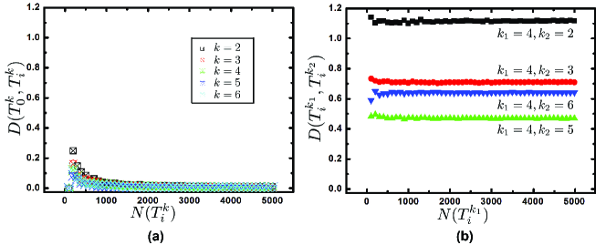
Figure 3: The spectral distance between $k-$regular trees with growing size. (a) Trees from the same subclass, (b) Trees from different subclasses with $k_{1}=4$.

We finally compare these graph classes with each other and with some of the graph classes such as complete (bipartite) graph, paths, cycles, or cubes, that have been discussed in the previous section.

All the graphs are generated with almost equal size, around 2000 (except for the $11-cube$ and $k-$regular graphs, the other graphs contain 2000 vertices). As mentioned before, the average degree can divide the $k-$regular trees into some sub-classes, so we organzine groups of graphs as their average degree ($\langle d\rangle$ is chosen from 4, 6, 8). The random graphs are obtained via the Erdős-Rényi random model (see [38, 39]), while the scale-free graphs are obtained via the Barabási-Albert scale-free model (see [35, 36]). With fixed average degree, 5 scale-free graphs and 5 random graphs are generated. For the $n-$cube or $k-$regular trees, we choose the nearest number to 2000, for example, we chose the $11-$cube, a $4-$regular tree with size 1457, a 6-regular tree with size 4687 and a 8-regular tree with size 3201. We calculate the spectral distance (Eq. 1.4) among graphs in one group, then color values in the distance matrix, as shown in Fig. 4.

In Fig. 4, a dark-blue square means that the spectral distance is almost 0. With fixed average degree (Fig. 4(a)-(c)), such squares among the 5 random, the 5 scale-free graphs, between the cycles and paths and between the complete graph and the complete bipartite graph. Moreover, the random graphs have small spectral distance to the scale-free graphs, and also to the path and cycle. Fig. 4(d) shows all the color squares above. In the group of random graphs, those with average degree 4 are nearer to scale-free ones with average degree 4 than to random ones with average degree 8, with respect to the spectral distance. A similar result obtains for the scale-free graphs. Thus, the average degree can be a dominant factor when comparing graphs through the spectral distance.

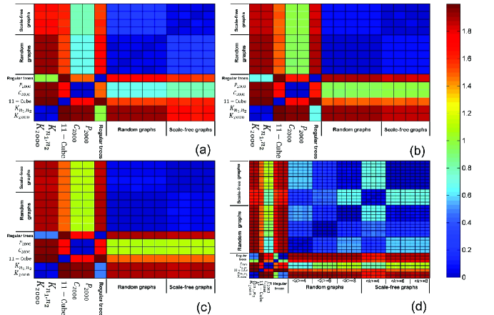
Figure 4: The spectral distance between empirical graphs and particular graphs, whose sizes are around 2000 and degrees are $\langle d\rangle=$4, 6, 8. (a) $\langle d\rangle=$4; (b) $\langle d\rangle=$6; (c) $\langle d\rangle=$8; (d) All plots taken from (a), (b) and (c).

In addition, we also take networks from empirical databases, such as biological networks (domain-domain co-occurrence networks) and linguistic networks (word-word co-occurrence networks). In biological networks, we choose the species B. taurus (2129 vertices, $\langle d\rangle=11.22$), D. melanogaster (1762 vertices, $\langle d\rangle=9.51$), G. gallus (1988 vertices, $\langle d\rangle=10.85$), R. norvegicus (2130 vertices, $\langle d\rangle=11.01$) and S. scrofa (1904 vertices, $\langle d\rangle=9.98$). The random graphs and scale-free graphs with similar parameters (2000 vertices, $\langle d\rangle=10$) are selected for comparison. Fig. 5(a) is the distance matrix composed of color squares. The biological networks are nearer to the random and scale-free graphs than to the regular graphs (such as cycle, path).

The linguistic networks (word-word co-occurrence networks) are generated from the corpora (Wortschatz) database [40]. In contrast to biological networks, linguistic networks are quite dense, with average degrees around 500. We chose 5 linguistic networks with 2000 vertices: German ($\langle d\rangle=512.83$), English ($\langle d\rangle=695.84$), Danish ($\langle d\rangle=505.94$), Norwegian ($\langle d\rangle=490.04$) and Swedish ($\langle d\rangle=481.7$). In Fig. 5(b), linguistic networks are nearer to the random graphs than to the other graphs. Since they are quite dense, as a typical vertex is connected with around one quarter of the vertices in the whole network, they are nearer to the complete graph and to the complete bipartite graph than to the other regular graphs.

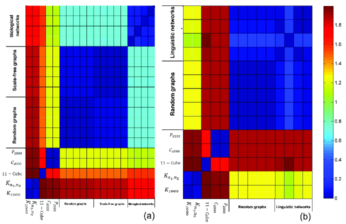
Figure 5: The spectral distance between empirical graphs and networks from real database: (a) biological networks (domain-domain co-occurrence networks) (b) linguistic networks (word-word co-occurrence networks).

References

- [1] D. Conte, P. Foggia, C. Sansone and M. Vento. Thirty years of graph matching in pattern recognition, International journal of pattern recognition and artificial intelligence, 18. 3, (2004), 265-298.
- [2] H. Bunke and K. Shearer, A graph distance metric based on the maximal common subgraph, Pattern recognition letters, 19, 3, (1998), 255-259.
- [3] J. Berg and M. Lässig, Cross-species analysis of biological networks by Bayesian alignment, Proceedings of the National Academy of Sciences, 103, 29, (2006), 10967-10972.
- [4] W. L. Chen, D. Z. Chen and K. T. Taylor, Automatic reaction mapping and reaction center detection, Wiley Interdisciplinary Reviews: Computational Molecular Science, 3, 6, (2013), 560-593.
- [5] S. A. Cook, The complexity of theorem-proving procedures, Proceedings of the third annual ACM symposium on Theory of computing, (1971), 151-158.
- [6] R. C. Read and D. G. Corneil, The graph isomorphism disease, Journal of Graph Theory, 1, 4, (1977), 339-363.
- [7] L. Bahiense, G. Manić, B. Piva and C. C. de Souza, The maximum common edge subgraph problem: a polyhedral investigation, Discrete Appl. Math., 160, 18, (2012), 2523-2541.
- [8] S. V. N. Vishwanathan, N. N. Schraudolph, R. Kondor and K. M. Borgwardt, Graph kernels, Journal of Machine Learning Research, 11, (2010), 1201-1242.
- [9] K. Kundu, F. Costa and R. Backofen, A graph kernel approach for alignment-free domain–peptide interaction prediction with an application to human SH3 domains, Bioinformatics, 29, 13 (2013), i335-i343.
- [10] L. Ralaivola, S. J. Swamidass, H. Saigo and P. Baldi, Graph kernels for chemical informatics, Neural Networks, 18, 8, (2005), 1093-1110.
- [11] O. Macindoe and W. Richards, Graph comparison using fine structure analysis, Proceedings of the 2010 IEEE Second International Conference on Social Computing, (2010), 193-200.
- [12] F. Chung, Spectral graph theory, American Mathematical Society, 92, 1997.
- [13] J. Jost and M. P. Joy, Spectral properties and synchronization in coupled map lattices, Physical Review E, 65, 1, (2001), 016201.
- [14] A. A. Ranicki, Algebraic L-theory and topological manifolds, Cambridge University Press, 102, 1992.
- [15] F. Bauer, J Jost and S. P. Liu, Ollivier–Ricci curvature and the spectrum of the normalized graph Laplace operator, Mathematical Research Letters, 19, 6, (2012), 1185-1205.
- [16] D. Horak and J. Jost, Interlacing inequalities for eigenvalues of discrete Laplace operators, Annals of Global Analysis and Geometry, 43, 2, (2013), 177-207.
- [17] A. Banerjee, The spectrum of the graph Laplacian as a tool for analyzing structure and evolution of networks, PhD thesis, University of Leipzig, 2008.
- [18] M. Mario Thüne, Eigenvalues of matrices and graphs, PhD thesis, University of Leipzig, 2012.
- [19] D. Stevanović, Research problems from the Aveiro workshop on graph spectra, Linear Algebra and its Applications, 423, 1, (2007), 172-181.
- [20] I. Jovanović and Z. Stanić, Spectral distances of graphs, PLinear Algebra and its Applications, 436, 5, (2012), 1425-1435.
- [21] W. Wang and C. X. Xu, On the asymptotic behavior of graphs determined by their generalized spectra, Discrete Mathematics, 310, 1, (2010), 70-76.
- [22] M. Rosenblatt, Remarks on some nonparametric estimates of a density function, The Annals of Mathematical Statistics, 27, 3, (1956), 832-837.
- [23] E. Parzen, On estimation of a probability density function and mode, The annals of mathematical statistics, 33, 3, (1962), 1065-1076.
- [24] D. Horak and J. Jost, Spectra of combinatorial Laplace operators on simplicial complexes, Adv.Math., 244, (2013), 303-336.
- [25] E. P. Wigner, Characteristic vectors of bordered matrices with infinite dimensions, The Annals of Mathematics, 65, 2, (1955), 203-207.
- [26] E. P. Wigner, Characteristic vectors of bordered matrices with infinite dimensions II, The Annals of Mathematics, 62, 3, (1955), 548-564.
- [27] E. P. Wigner, On the distribution of the roots of certain symmetric matrices, The Annals of Mathematics, 67, 2, (1958), 325–327.
- [28] A. Banerjee and J. Jost, Spectral plot properties: Towards a qualitative classification of networks, Networks and heterogeneous media, 3, 2, (2008), 395-411.
- [29] L. Lovász, Large networks and graph limits, American Mathematical Society colloquium publications, 60, American Mathematical Society, 2012.
- [30] H. Robbins, A remark on Stirling’s formula, American Mathematical Monthly, 62, 1, (1955), 26-29.
- [31] A. Banerjee and J. Jost, On the spectrum of the normalized graph Laplacian, Linear Algebra and its Applications, 428, 11-12, (2008), 3015-3022.
- [32] Y. V. Prohorov, Convergence of random processes and limit theorems in probability theory, Teor. Veroyatnost. i Primenen. 1, (1956), 177-238.
- [33] W. H. Haemers, Interlacing eigenvalues and graphs, Linear Algebra and its Applications, 226, 3, (1995), 593-616.
- [34] G. T. Chen, G. Davis, F. Hall, Z. S. Li, K. Patel and M. Stewart, An interlacing result on normalized Laplacians, SIAM Journal on Discrete Mathematics, 18, 2, (2004), 353-361.
- [35] A. L. Barabási and R. Albert, Emergence of scaling in random networks, Science, 286, 5439, (1999), 509-512.
- [36] S. N. Dorogovtsev, J. F. Mendes and A. N. Samukhin, Structure of growing networks with preferential linking, Physical Review Letters, 85, 21, (2000), 4633-4636.
- [37] F. Chung, L. Y. Lu and V. Vu, Spectra of random graphs with given expected degrees, Proceedings of the National Academy of Sciences of the United States of America, 100, 11, (2003), 6313-6318.
- [38] P. Erdős and A. Rényi, On random graphs I, Publicationes Mathematicae Debrecen, 6, (1959), 290-297.
- [39] P. Erdős and A. Rényi, On the evolution of random graphs, Bull. Inst. Internat. Statist., 38, (1961), 343-347.
- [40] U. Quasthoff, M. Richter and C. Biemann, Corpus portal for search in monolingual corpora, Proceedings of the fifth international conference on language resources and evaluation, (2006), 1799-1802.