Supersymmetric heterotic solutions via non-$SU(3)$ standard embedding

Abstract

A supersymmetric solution to type II supergravity is constructed by superposing two hyper-Kählers with torsion metrics. The solution is given by a Kähler with torsion metric with $SU(3)$ holonomy. The metric is embedded into a heterotic solution obeying the Strominger system, together with a Yang–Mills instanton obtained by the standard embedding. T dualities lead to an $SO(6)$ instanton describing a symmetry breaking from $E_{8}$ to $SO(10)$. The compactification by taking a periodic array yields a supersymmetric domain wall solution of heterotic supergravity.

I Introduction

The Green–Schwarz mechanism GSmechanism is one of the cornerstones of superstring theory. Its role is twofold: First, of course, is to tell us how to cancel the gauge and gravitational anomalies of ten-dimensional type I and heterotic superstrings, which were apparently considered anomalous and hence unacceptable as consistent theories. With the mechanism, however, it turned out that all the anomalies were canceled out in a miraculous manner if and only if the gauge group was $SO(32)$ or $E_{8}\times E_{8}$, for the latter of which heterotic string theory has been constructed heterotic_string .

The second important role of the Green–Schwarz mechanism is to constrain the background geometry through the modified Bianchi identity of the 3-form field $H$; the mechanism requires the 2-form $B$ field to vary under both the gauge and local Lorentz transformations so that the invariant 3-form field $H$ must be of the form

$$H=dB-\alpha^{\prime}\left({\omega}_{3Y}-{\omega}_{3L}^{-}\right),$$ (1)

where ${\omega}_{3Y}$ is the Chern–Simons 3-form associated with the Yang–Mills connection, and ${\omega}_{3L}^{-}$ is also a Chern–Simons 3-form but made of a particular linear combination of the Levi-Civit$\acute{\text{a}}$ connection and the 3-form field:

$$\omega^{-}_{MAB} = \omega_{MAB}-H_{MAB}.$$ (2)

The equation (1) leads to the Bianchi identity

$$dH=\alpha^{\prime}\left(tr\mathcal{F}\wedge\mathcal{F}-tr\mathcal{R}^{-}\wedge\mathcal{R}^{-}\right).$$ (3)

This constrains the background geometry GSW in such a way that the second Chern class of the gauge bundle be equal to the first Pontryagin class of the tangent bundle including torsion as in (2).

Note that the combination (2) is different from the one that appears in the supersymmetry(SUSY) variation of the gravitino

$$\delta\psi_{M} \propto \nabla^{+}\varepsilon,$$ (4)

where $\nabla^{+}$ is the covariant derivative associated with the combination

$$\omega^{+}_{MAB} = \omega_{MAB}+H_{MAB}.$$ (5)

The relevance of the difference between the two connections was pointed out by Bergshoeff and de Roo BdR , and later emphasized by e.g., Refs. KimuraYi ; MS .

For $E_{8}\times E_{8}$ heterotic string theory on a six-dimensional space $M^{6}$ without $H$ fluxes, the Killing spinor equation arising from the vanishing gravitino variation (4) constrains $M^{6}$ to have $SU(3)$ holonomy, that is, to be Calabi–Yau. On the other hand, for the Bianchi identity (3) to be satisfied, the easiest and most common way is to set the $\omega^{+}$ connection, which is nothing but the spin (Levi-Civit$\acute{\text{a}}$) connection for $H=0$, to be equal to a part of the gauge connection. This is called the standard embedding Witten_New_Issues . In this case, a part of the gauge field background is required to be $SU(3)$, and the gauge symmetry is partially broken to the centralizer $E_{6}(\times E_{8})$. This reduction of the gauge symmetry is one of the hallmarks of Calabi–Yau compactifications of heterotic string theory.

If, on the other hand, there is a nonzero $H$ field, then the vanishing gravitino variation (4) asserts that the linear combination $\omega^{+}_{MAB}=\omega_{MAB}+H_{MAB}$ belongs to $SU(3)$ but says nothing about the other linear combination $\omega^{-}_{MAB}=\omega_{MAB}-H_{MAB}$ Strominger ; BdR ; KimuraYi . Thus $\omega^{-}_{MAB}$ is generically in $SO(6)$ on the six-dimensional space $M^{6}$, and the gauge symmetry is broken to a smaller subgroup $SO(10)$, which is more favorable from the point of view of applications to string phenomenology. Note that, in the presence of $H$ fluxes, $SO(10)$ is achieved by the “standard embedding”, that is, by simply equating the modified spin connection $\omega^{-}_{MAB}$ with a part of the gauge connection. This is in striking contrast to the $H=0$ Calabi–Yau case, in which one needs the nonstandard embedding that requires complicated mathematical machinery Witten_New_Issues ; GSW involving the construction of stable holomorphic vector bundles.

However, for the smeared intersecting NS5-brane solution, which is obtained as a superposition of two smeared symmetric 5-brane solutions CHS and is one of the simplest SUSY heterotic supergravity solutions with $H$ fluxes in the six-dimensional space, not only $\omega^{+}$ but also $\omega^{-}$ happens to be in $SU(3)$, and therefore the unbroken gauge symmetry is still $E_{6}$. The reason for this can be traced back to the parity invariance of the symmetric 5-brane solution; indeed, the sign of $H$ is a matter of convention, and the configuration after the sign flip $H\rightarrow-H$ still remains a solution of the heterotic supergravity.

In this paper, we construct a supersymmetric heterotic supergravity solution such that $\omega^{+}$ is in $SU(3)$ (and hence a SUSY solution) but $\omega^{-}$ is not , by superposing two hyper-Kählers with torsion (HKT) geometries. As already pointed out in Ref. CHS , one can obtain HKT geometries by conformally transforming hyper-Kähler geometries. We choose the Gibbons–Hawking space as the starting point and apply a conformal transformation to obtain a HKT geometry. Since the Gibbons–Hawking space is not parity invariant, the $\omega^{-}$ connection of the resulting HKT space is in $SO(4)$ but not in $SU(2)$, though $\omega^{+}$ still belongs to $SU(2)$.

We then smear the harmonic functions to those of two dimensions and take a superposition of two such geometries. Because of our superposition ansatz, we are forced to set some of the entries of the metric to zero in order to satisfy the equations of motion. Consequently, we find that the $\omega^{-}$ holonomy of the superposed solution remains to be $SO(4)$. We also show that by T duality this solution turns into one with $SO(5)$ or $SO(6)$ $\omega^{-}$ holonomy.

We also take a two-dimensional periodic array of the “intersecting HKT” solutions to get a compact six-dimensional solution. We find that the fundamental parallelogram of the two-dimensional periodic array is separated into distinct smooth regions bordered by codimension-1 singularity hypersurfaces, hence the name “supersymmetric domain wall.” This novel solution has some interesting properties, as we will see below.

This paper is organized as follows. In Sec. II, we give a brief review of HKT geometries obtained by conformal transformations acting on four-dimensional hyper-Kähler spaces. In Sec. III, we consider a superposition of HKT spaces to construct a six-dimensional Kähler with torsion (KT) space with special properties which serves as a supersymmetric solution of type II supergravity. In Sec. IV, we embed this geometry into heterotic supergravity theory and take T dualities. In Sec. V, we compactify this six-dimensional space by taking a periodic array and study some of its properties. The final section presents the summary and conclusion.

II HKT geometry as a conformal transform

We start with a four-dimensional HKT metric ${g}_{HKT}$ obtained as a conformal transform of a hyper-Kähler metric, where for the latter we specifically consider the Gibbons–Hawking (GH) metric ${g}_{GH}$,

$${g}_{HKT}=\Phi\,{g}_{GH}.$$ (6)

The GH metric is given by GH

$${g}_{GH}=\frac{1}{\phi}\left(d\tau-\sum_{i=1}^{3}\psi_{i}dx^{i}\right)^{2}+\phi\sum_{i=1}^{3}(dx^{i})^{2},$$ (7)

where $\phi$ and $\textrm{\boldmath$\psi$}=(\psi_{1},\psi_{2},\psi_{3})$ are scalar functions of the coordinates $(x^{1},x^{2},x^{3})$ of ${\bf{R}}^{3}$ obeying the relation

$$\mbox{grad}\,\phi=\mbox{rot}\,\textrm{\boldmath$\psi$}.$$ (8)

$\Phi$ is a scalar field of which the properties will be described shortly. We define the orthonormal basis

$${E}^{0}=\sqrt{\frac{\Phi}{\phi}}\left(d\tau-\sum_{i=1}^{3}\psi_{i}dx^{i}\right),~{}{E}^{i}=\sqrt{\Phi\,\phi}\,dx^{i}~{}(i=1,2,3)$$ (9)

so that the hypercomplex structure is given by the three complex structures ${J}^{a}~{}(a=1,2,3)$ satisfying the quaternionic identities,

$${J}^{a}({E}^{\mu})=\bar{\eta}^{a}_{\mu\nu}{E}^{\nu},$$ (10)

where $\bar{\eta}^{a}_{\mu\nu}$ are the ’t Hooft matrices. The corresponding fundamental 2-forms are

$${\Omega}^{a}=-\bar{\eta}^{a}_{\mu\nu}{E}^{\mu}\wedge{E}^{\nu}.$$ (11)

The HKT structure is defined by the 3-form torsion $T$ satisfying HP96 GP00

$$T={J}^{1}d{\Omega}^{1}={J}^{2}d{\Omega}^{2}={J}^{3}d{\Omega}^{3}.$$ (12)

In the present case, we have

$$T=-{E}_{0}\log\Phi{E}^{123}+{E}_{1}\log\Phi{E}^{023}+{E}_{2}\log\Phi{E}^{031}$$

$$~{}~{}~{}~{}~{}~{}+{E}_{3}\log\Phi{E}^{012}$$ (13)

in terms of dual vector fields ${E}_{\mu}$ to the 1-forms (9),

$${E}_{0}=\sqrt{\frac{\phi}{\Phi}}\frac{\partial}{\partial\tau},~{}~{}{E}_{i}=\frac{1}{\sqrt{\Phi\,\phi}}\left(\frac{\partial}{\partial x^{i}}+\psi_{i}\frac{\partial}{\partial\tau}\right)$$ (14)

and

$${E}^{\mu\nu\lambda}={E}^{\mu}\wedge{E}^{\nu}\wedge{E}^{\lambda}.$$ (15)

The exterior derivative is calculated as

$$dT=-\frac{1}{\Phi^{2}\phi}\left(\sum_{\mu=0}^{3}{V}_{\mu}^{2}\Phi\right){E}^{0123}$$ (16)

with the vector fields ${V}_{\mu}=\sqrt{\Phi\,\phi}\,{E}_{\mu}$. Therefore, if $\Phi$ is chosen to be a harmonic function with respect to the GH metric (7), then the torsion $T$ becomes a closed 3-form.

Using this $T$, we introduce the two types of connections $\nabla^{\pm}$,

$$\nabla^{\pm}_{X}Y=\nabla_{X}Y\pm\frac{1}{2}\sum_{\mu=0}^{3}T(X,Y,E_{\mu})E_{\mu},\,$$ (17)

where $\nabla$ is a Levi-Civitá connection. The corresponding connection 1-forms $\mathcal{\omega}^{\pm\,\mu}_{~{}~{}~{}\nu}$ are defined by

$$\nabla^{\pm}_{E_{\mu}}{E}_{\nu}=\mathcal{\omega}^{\pm\,\lambda}_{~{}~{}~{}\nu}(E_{\mu}){E}_{\lambda},$$ (18)

and the curvature 2-forms are written as

$$\mathcal{R}^{\pm\,\mu}_{~{}~{}~{}\nu}=d\mathcal{\omega}^{\pm\,\mu}_{~{}~{}~{}\nu}+\mathcal{\omega}^{\pm\,\mu}_{~{}~{}~{}\lambda}\wedge\mathcal{\omega}^{\pm\,\lambda}_{~{}~{}~{}\nu}.$$ (19)

The torsion curvature $\mathcal{R}^{+\,\mu}_{~{}~{}~{}\nu}$ satisfies the $SU(2)$ holonomy condition

$$\mathcal{R}^{+}_{~{}~{}01}+\mathcal{R}^{+}_{~{}~{}23}=0,~{}\mathcal{R}^{+}_{~{}~{}02}+\mathcal{R}^{+}_{~{}~{}31}=0,~{}\mathcal{R}^{+}_{~{}~{}03}+\mathcal{R}^{+}_{~{}~{}12}=0.$$ (20)

On the other hand, if the torsion $T$ is a closed 3-form, that is, $\Phi$ is a harmonic function, then the curvature $\mathcal{R}^{-\,\mu}_{~{}~{}~{}\nu}$ becomes an anti self dual 2-form, which may be regarded as a Yang–Mills instanton with the gauge group $SU(2)\times SU(2)=SO(4)$.

III Intersecting HKT metrics

In the previous section we have seen that the HKT metrics obtained by a conformal transformation have $\mathcal{\omega}^{+\,\mu}_{~{}~{}~{}\nu}$ in $SU(2)$ but $\mathcal{\omega}^{-\,\mu}_{~{}~{}~{}\nu}$ in $SO(4)$ strictly larger than $SU(2)$ as long as the original GH space is not a flat Euclidean space. In this section we construct their six-dimensional analogs by superposing two such HKT metrics embedded in different four-dimensional subspaces. This construction is motivated by that used in constructing intersecting brane solutions AEH ; O ; namely, we assume the form of the metric as

$$g=\Phi\tilde{\phi}\phi\tilde{\phi}((dx^{1})^{2}+(dx^{2})^{2})+\Phi\phi(dx^{3})^{2}$$

$$~{}~{}~{}~{}+\frac{\Phi}{\phi}(dx^{4}-\psi dx^{3})^{2}+\tilde{\Phi}\tilde{\phi}(dx^{5})^{2}+\frac{\tilde{\Phi}}{\tilde{\phi}}(dx^{6}-\tilde{\psi}dx^{5})^{2}.$$

The HKT metric that we have considered in the previous section is characterized by a triplet $(\Phi,\phi,\psi)$ on ${\bf{R}}^{3}=\{(x^{1},x^{2},x^{3})\}$ obeying (8). So at first it might seem that $(\Phi,\phi)$ or $(\tilde{\Phi},\tilde{\phi})$ could to be functions of $(x^{1},x^{2},x^{3})$ or $(x^{1},x^{2},x^{5})$, and $dx^{4}-\psi dx^{3}$ or $dx^{6}-\tilde{\psi}dx^{5}$ could be replaced with a more general form $dx^{4}-\sum_{i=1,2,3}\psi_{i}dx^{i}$ or $dx^{6}-\sum_{i=1,2,5}\tilde{\psi}_{i}dx^{i}$, respectively. However, it turns out that such a more general ansatz does not lead to a metric with $SU(3)$ holonomy even in the case $\Phi=\tilde{\Phi}=1$. Thus we are led to consider the metric of the form (III), assuming the following:

• $(\Phi,\phi)$ and $(\tilde{\Phi},\tilde{\phi})$ are harmonic functions on the two-dimensional flat space ${\bf{R}^{2}}=\{(x^{1},x^{2})\}$.

• $\textrm{\boldmath$\psi$}=(0,0,\psi)$ and $\textrm{\boldmath$\tilde{\psi}$}=(0,0,\tilde{\psi})$ , of which the components are harmonic functions on ${\bf{R}^{2}}$ satisfying the Cauchy–Riemann conditions

  $$\frac{\partial\phi}{\partial x_{2}} = -\frac{\partial\psi}{\partial x_{1}},~{}~{}~{}\frac{\partial\phi}{\partial x_{1}}=\frac{\partial\psi}{\partial x_{2}},$$

  $$\frac{\partial\tilde{\phi}}{\partial x_{2}} = -\frac{\partial\tilde{\psi}}{\partial x_{1}},~{}~{}~{}\frac{\partial\tilde{\phi}}{\partial x_{1}}=\frac{\partial\tilde{\psi}}{\partial x_{2}}.$$ (22)

Under these assumptions, we will show that a six-dimensional space $M^{6}$ with the metric (III) has the following KT structure:

• a closed Bismut torsion [see Eq. (III)],

• an exact Lee form [see Eq. (28)],

• a Bismut connection $\nabla^{+}$ with $SU(3)$ holonomy [see Eq. (29)].

We first introduce an orthonormal basis

$${e}^{1}=\sqrt{\Phi\tilde{\Phi}\phi\tilde{\phi}}dx^{1}\;,\;{e}^{2}=\sqrt{\Phi\tilde{\Phi}\phi\tilde{\phi}}dx^{2}\,,$$

$${e}^{3}=\sqrt{\Phi\phi}dx^{3}\;,\;{e}^{4}=\sqrt{\frac{\Phi}{\phi}}(dx^{4}-\psi dx^{3})\,,$$

$${e}^{5}=\sqrt{\tilde{\Phi}\tilde{\phi}}dx^{5}\;,\;{e}^{6}=\sqrt{\frac{\tilde{\Phi}}{\tilde{\phi}}}(dx^{6}-\tilde{\psi}dx^{5})\,.$$ (23)

The space $M^{6}$ has a natural complex structure $J$ defined by

$$J({e}^{1})=\epsilon_{1}{e}^{2}\,,\,J({e}^{3})=\epsilon_{2}{e}^{4}\,,\,J({e}^{5})=\epsilon_{3}{e}^{6}\,.$$ (24)

Indeed, it is easy to see that the Nijenhuis tensor associated with $J$ vanishes under the condition $|\epsilon_{i}|=1(i=1,2,3)$ and $\epsilon_{1}\epsilon_{2}=\epsilon_{1}\epsilon_{3}=-1$. Then, the metric (III) becomes Hermitian with respect to the complex structure $J$, and the fundamental 2-form $\kappa$ takes the form

$$\kappa=\epsilon_{1}{e}^{1}\wedge{e}^{2}+\epsilon_{2}{e}^{3}\wedge{e}^{4}+\epsilon_{3}{e}^{5}\wedge{e}^{6}\,.$$ (25)

The Bismut torsion $T$ is uniquely determined by

$$\nabla^{+}_{X}g=0\;,\;\nabla^{+}_{X}\kappa=0\,.$$ (26)

Explicitly we have

$$T=-J\,d\kappa$$

$$~{}~{}=\frac{1}{\Phi\sqrt{\Phi\tilde{\Phi}\phi\tilde{\phi}}}(\partial_{1}\Phi e^{234}-\partial_{2}\Phi e^{134})$$

$$~{}~{}~{}~{}~{}~{}~{}+\frac{1}{\tilde{\Phi}\sqrt{\Phi\tilde{\Phi}\phi\tilde{\phi}}}(\partial_{1}\tilde{\Phi}e^{256}-\partial_{2}\tilde{\Phi}e^{156}).$$ (27)

It should be noticed that in our case the Bismut torsion is a closed 3-form, $dT=0$. We shall refer to $\nabla^{+}$ and $\nabla^{-}$ as the Bismut connection and Hull connection, respectively, according to Ref. MS . The Lee form $\theta$ is a 1-form defined by $\theta=-J\delta\kappa$ IP , which becomes a closed 1-form,

$$\theta=2d\varphi,~{}~{}~{}\varphi=\log\sqrt{\Phi\tilde{\Phi}}.$$ (28)

We will identify the Bismut torsion with 3-form flux, $T=H$, and the function $\varphi$ with a dilaton. It is shown that the Ricci form IP of the Bismut connection vanishes, which is equivalent to the condition

$$\epsilon_{1}\mathcal{R}^{+}_{~{}12}+\epsilon_{2}\mathcal{R}^{+}_{~{}34}+\epsilon_{3}\mathcal{R}^{+}_{~{}56}=0,$$ (29)

so that the holonomy of $\nabla^{+}$ is contained in $SU(3)$ and $M^{6}$ admits two independent Weyl Killing spinors obeying $\nabla^{+}_{X}\varepsilon=0$ in type II theory. Thus the triplet $(g,H,\varphi)$ gives rise to a supersymmetric solution to the type II supergravity theory.

IV Embedding into heterotic string theory and T duality

We study supersymmetric solutions describing heterotic flux compactification. The bosonic part of the string frame action, up to the first order in the $\alpha$’ expansion, is given by

$$S = \frac{1}{2\kappa^{2}}\int d^{10}x\sqrt{-g}e^{-2\varphi}\left(R+4(\nabla\varphi)^{2}\right.$$ (30)

$$-\frac{1}{12}H_{MNP}H^{MNP}$$

$$\left.-\alpha^{\prime}(tr\mathcal{F}_{MN}\mathcal{F}^{MN}-tr\mathcal{R}^{-}_{MN}\mathcal{R}^{-MN})\right).$$

It is assumed that ten-dimensional spacetimes take the form $R^{1,3}\times M^{6}$, where $M^{6}$ is a six-dimensional space admitting a Killing spinor $\varepsilon$,

$$\nabla^{+}_{a}\varepsilon=0,~{}~{}\left(\gamma^{a}\partial_{a}\varphi+\frac{1}{12}H_{abc}\gamma^{abc}\right)\varepsilon=0,~{}~{}\mathcal{F}_{ab}\gamma^{ab}\varepsilon=0.$$ (31)

This system together with the anomaly cancellation condition

$$dH=\alpha^{\prime}\left(tr\mathcal{F}\wedge\mathcal{F}-tr\mathcal{R}^{-}\wedge\mathcal{R}^{-}\right)$$ (32)

is known as the Strominger system Strominger .

Now, we turn to the heterotic solution obeying the Strominger system. If the curvature $\mathcal{R}^{-}$ in the anomaly condition (32) is given by the Hull connection $\nabla^{-}$, we can choose a non-Abelian gauge field as $\mathcal{F}=\mathcal{R}^{-}$ since the 3-form flux (III) is closed by the identification $T=H$. This is a form of the usual standard embedding. Combining the well-known identity

$$\mathcal{R}^{+}_{abcd}-\mathcal{R}^{-}_{cdab}=\frac{1}{2}(dT)_{abcd}=0$$ (33)

with the holonomy condition (29), we can see that the gauge field $\mathcal{F}$ is an instanton satisfying the third equation in (31).

Apparently, $\mathcal{F}$ seems to take values in $SO(6)$ $\subset$ $E_{8}$, which would describe a symmetry breaking from $E_{8}$ to $SO(10)$. However, for generic choices of the harmonic functions $\phi$, $\Phi$, $\tilde{\phi}$, and $\tilde{\Phi}$, it is not ensured that the metric (III) can remain non-negative, and the dilaton (28) can remain real valued. Therefore, to get a meaningful solution we are forced to impose

$$\phi=\tilde{\phi}=\Phi=\tilde{\Phi}.$$ (34)

With this condition, the holonomy of $\nabla^{+}$ remains $SU(3)$, but the instanton $\mathcal{F}$ reduces to a proper Lie subalgebra $SO(4)$ of $SO(6)$, and the centralizer is $SO(12)$.

To recover the $SO(6)$ instanton, we apply a T-duality transformation. From (III), (III), and (28), with $\phi=\tilde{\phi}=\Phi=\tilde{\Phi}$, we have the following metric with $SU(3)$ holonomy , 3-form flux, and dilaton:

$$g = \phi^{4}((dx^{1})^{2}+(dx^{2})^{2})+\phi^{2}(\,(dx^{3})^{2}+(dx^{5})^{2}\,)$$ (35)

$$+ (dx^{4}-\psi dx^{3})^{2}+(dx^{6}-\psi dx^{5})^{2},$$

$$H = -\frac{1}{\phi^{3}}(\partial_{2}\phi e^{134}-\partial_{1}\phi e^{234}+\partial_{2}\phi e^{156}-\partial_{1}\phi e^{256}),$$

(36)

$$\varphi = \log{|\phi|}.$$ (37)

The metric (35) has isometries $U(1)^{4}$ generated by Killing vector fields $\partial_{a}~{}~{}(a=3,4,5,6)$. Therefore, we can T dualize the type II solution $(g,H,\varphi)$ along directions of these isometries. It is easy to see that the solution is inert under the T duality along $x^{4}$ and $x^{6}$; the T dualities along the remaining directions give nontrivial deformations of the solutions, preserving one-quarter of supersymmetries.

We first T dualize the solution along $x^{3}$. The resulting solution $(\hat{g},\hat{H},\hat{\varphi})$ is given by

$$\hat{g} = \phi^{4}(\,(dx^{1})^{2}+(dx^{2})^{2}\,)+\frac{1}{\phi^{2}+\psi^{2}}(d\hat{x}^{3}+\psi dx^{4})^{2}$$ (38)

$$+\frac{\phi^{2}}{\phi^{2}+\psi^{2}}(dx^{4})^{2}+\phi^{2}(dx^{5})^{2}+(dx^{6}-\psi dx^{5})^{2}\,,$$

$$\hat{H} = \frac{1}{\phi^{3}(\phi^{2}+\psi^{2})}((\phi^{2}+\psi^{2})\partial_{2}\phi+2\psi(\phi\partial_{1}\phi-\psi\partial_{2}\phi)\,)\hat{e}^{134}$$ (39)

$$-\frac{1}{\phi^{3}(\phi^{2}+\psi^{2})}(\,(\phi^{2}+\psi^{2})\partial_{1}\phi-2\psi(\phi\partial_{2}\phi+\psi\partial_{1}\phi)\,)\hat{e}^{234}$$

$$-\frac{1}{\phi^{3}}(\partial_{2}\phi\hat{e}^{156}-\partial_{1}\phi\hat{e}^{256})\,,$$

$$\hat{\varphi} = \frac{1}{2}\log\left({\frac{1}{(\phi^{2}+\psi^{2})}\phi^{2}}\right)\,.$$ (40)

Here, the orthonormal basis is defined by

$$\hat{e}^{1}=\phi^{2}dx^{1}\;,\;\hat{e}^{2}=\phi^{2}dx^{2},$$

$$\hat{e}^{3}=\frac{1}{\sqrt{\phi^{2}+\psi^{2}}}\left(d\hat{x}^{3}+\psi dx^{4}\right)\;,\;\hat{e}^{4}=\frac{\phi}{\sqrt{\phi^{2}+\psi^{2}}}dx^{4},$$

$$\hat{e}^{5}=\phi dx^{5}\;,\;\hat{e}^{6}=dx^{6}-\psi dx^{5}\,.$$ (41)

Then, we have a deformed complex structure $\hat{J}$,

$$\hat{J}\hat{e}_{1}=\epsilon_{1}\hat{e}_{2}\;,\;\hat{J}\hat{e}_{3}=\epsilon_{2}\hat{e}_{4}\;,\;\hat{J}\hat{e}_{5}=\epsilon_{3}\hat{e}_{6}\,$$ (42)

with $|\epsilon_{i}|=1(i=1,2,3)$ and $\epsilon_{1}\epsilon_{2}=\epsilon_{1}\epsilon_{3}=-1$. The associated fundamental two-form $\hat{\kappa}$ takes the same form as (25), and the Bismut connection $\nabla^{+}$ has an $SU(3)$ holonomy. In this case, it turns out that the Hull connection $\nabla^{-}$ is in $SO(5)$, which is still smaller than $SO(6)$.

Thus, we further T dualize the solution $(\hat{g},\hat{H},\hat{\varphi})$ once more along $x^{5}$ and finally obtain $(\tilde{g},\tilde{H},\tilde{\varphi})$:

$$\tilde{g}=\phi^{4}(\,(dx^{1})^{2}+(dx^{2})^{2}\,)+\frac{1}{\phi^{2}+\psi^{2}}(d\hat{x}^{3}+\psi dx^{4})^{2}$$

$$~{}+\frac{1}{\phi^{2}+\psi^{2}}(d\tilde{x}^{5}+\psi dx^{6})^{2}+\frac{\phi^{2}}{\phi^{2}+\psi^{2}}((dx^{4})^{2}+(dx^{6})^{2}),$$

$$\tilde{H}=\frac{1}{\phi^{3}(\phi^{2}+\psi^{2})}((\phi^{2}+\psi^{2})\partial_{2}\phi+2\psi(\phi\partial_{1}\phi-\psi\partial_{2}\phi))\tilde{e}^{134}$$

$$-\frac{1}{\phi^{3}(\phi^{2}+\psi^{2})}(\,(\phi^{2}+\psi^{2})\partial_{1}\phi-2\psi(\phi\partial_{2}\phi+\psi\partial_{1}\phi))\tilde{e}^{234}$$

$$+\frac{1}{\phi^{3}(\phi^{2}+\psi^{2})}((\phi^{2}+\psi^{2})\partial_{2}\phi+2\psi(\phi\partial_{1}\phi-\psi\partial_{2}\phi))\tilde{e}^{156}$$

$$-\frac{1}{\phi^{3}(\phi^{2}+\psi^{2})}((\phi^{2}+\psi^{2})\partial_{1}\phi-2\psi(\phi\partial_{2}\phi+\psi\partial_{1}\phi))\tilde{e}^{256},$$

$$\tilde{\varphi}=\frac{1}{2}\log\left(\frac{1}{(\phi^{2}+\psi^{2})(\phi^{2}+\psi^{2})}\phi^{2}\right)\,.$$ (45)

The orthonormal basis is defined by

$$\tilde{e}^{1}=\hat{e}^{1}\;,\;\tilde{e}^{2}=\hat{e}^{2}\,,\,\tilde{e}^{3}=\hat{e}^{3}\;,\;\tilde{e}^{4}=\hat{e}^{4}\,$$

$$\tilde{e}^{5}=\frac{1}{\sqrt{\phi^{2}+\psi^{2}}}(d\tilde{x}^{5}+\psi dx^{6})\;,\;\tilde{e}^{6}=\frac{\phi}{\sqrt{\phi^{2}+\psi^{2}}}dx^{6}\,.$$

In this basis the complex structure $\tilde{J}$ is given by

$$\tilde{J}\tilde{e}^{1}=\epsilon_{1}\tilde{e}^{2}\;,\;\tilde{J}\tilde{e}^{3}=\epsilon_{2}\tilde{e}^{4}\;,\;\tilde{J}\tilde{e}^{4}=\epsilon_{3}\tilde{e}^{2}\,$$ (47)

with $|\epsilon_{i}|=1(i=1,2,3)$ and $\epsilon_{1}\epsilon_{2}=\epsilon_{1}\epsilon_{3}=-1$. It can be verified that this solution has an $SU(3)$ Bismut connection $\nabla^{+}$ and $SO(6)$ Hull connection $\nabla^{-}$ as desired.

V SUSY domain wall metric

The last topic concerns the construction of type II/heterotic supersymmetric solutions on a compact six-dimensional space with the Hull connection not being in $SU(3)$. Since the triples obtained in the previous section depend only on $x^{1}$ and $x^{2}$, we can compactify the $x^{3}$, $x^{4}$, $x^{5}$ and $x^{6}$ spaces on $T^{4}$ by simply identifying periodically, whereas we consider a periodic array of copies of the solution along the $x^{1}$ and $x^{2}$ directions.

Let us consider a periodic array of $(g,H,\varphi)$ [Eqs. (35), (36), and (37)], $(\hat{g},\hat{H},\hat{\varphi})$ [(38), (39), and (40)], or $(\tilde{g},\tilde{H},\tilde{\varphi})$ [(IV), (IV), and (45)], which are characterized by a pair of harmonic functions $\phi$ and $\psi$. In two dimensions both the real and imaginary parts of any holomorphic function are harmonic. Thus we can take $\phi$ to be, say, the real part of any doubly periodic, holomorphic function. In this case, $\psi$ may be taken to be the imaginary part of the same doubly periodic function.

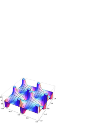
Figure 1: The real (upper plot) and imaginary (lower plot) parts of the $\wp$ function. The fundamental parallelogram can be taken to be $-\frac{1}{2}\leq\frac{x^{1}}{l}\leq\frac{1}{2}$ and $-\frac{1}{2}\leq\frac{x^{2}}{l}\leq\frac{1}{2}$.

Since the only nonsingular holomorphic function on $T^{2}$ is a constant function, we need to allow some pole singularities in the fundamental parallelogram of the periodic array, which may be seen to be in accordance with the no-go theorems against smooth flux compactifications GKP ; KimuraYi . The doubly periodic meromorphic functions are known as elliptic functions. It is well known that, for a given periodicity, the field of elliptic functions is generated by Weierstrass’s $\wp$ function and its derivative $\wp^{\prime}$. In the following, we consider, as a typical example, the compactification of $(g,H,\varphi)$, $(\hat{g},\hat{H},\hat{\varphi})$, and $(\tilde{g},\tilde{H},\tilde{\varphi})$ on a square torus of side $l$ by taking

$$\phi(x^{1},x^{2}) = \mbox{Re}~{}{\wp}(z),$$ (48)

$$\psi(x^{1},x^{2}) = \mbox{Im}~{}{\wp}(z),$$ (49)

where $\wp(z)$ is of modulus $\tau=i$ or $\tau=e^{\frac{\pi i}{5}}$ and $z=l^{-1}(x^{1}+ix^{2})$. Our solutions are determined entirely by Weierstrass’s $\wp$ function without any reference to $\alpha^{\prime}$ because of the choice $\mathcal{F}=\mathcal{R}^{-}$ that causes the rhs of (32) to be closed. Note that they solve the heterotic equations of motion up to $\mathcal{O}(\alpha^{\prime})$.

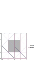
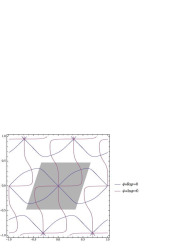
Figure 2: The zero loci of the real and imaginary parts of the $\wp$ function for the modulus $\tau=i$ (upper plot) and $\tau=e^{\frac{\pi i}{5}}$ (lower plot). The shaded region is the fundamental parallelogram.

The real and imaginary parts of $\wp(z)$ are shown in Fig. 1. We see that $\phi$ may take negative as well as positive values, but note that the metric (35), (38), or (38) depends on $\phi$ through $\phi^{2}$ as we designed, so the solution is only singular where $\phi$ vanishes (as well as $\phi$ diverges). Also, negative $\psi$ causes no problem as long as $\phi$ is nonzero.

For any case of $(g,H,\varphi)$, $(\hat{g},\hat{H},\hat{\varphi})$, or $(\tilde{g},\tilde{H},\tilde{\varphi})$, some of the components of the metric vanish where $\phi=0$, and hence the solution is singular. Also, the “string coupling” (= exponential of the dilaton) vanishes there. The $\phi=0$ curves are shown in Fig. 2 for the cases $\tau=i$ and $\tau=e^{\frac{\pi i}{5}}$. For both cases, we see that the fundamental parallelogram (shown by the shaded region) is separated into two distinct smooth regions bordered by the codimension-1 singularity hypersurfaces. The two singularity hypersurfaces intersect at $x^{1}=x^{2}=0$, where the $\wp$ function has a unique double pole; its real and imaginary parts rapidly fluctuate at $x^{1}=x^{2}=0$. More details about the solution will be reported elsewhere.

VI Conclusions

In this paper we have shown that two HKT metrics given by $(\Phi,\phi,\textrm{\boldmath$\psi$})$ and $(\tilde{\Phi},\tilde{\phi},\tilde{\textrm{\boldmath$\psi$}})$ can be superposed and lifted to a six-dimensional smeared intersecting solution of type II supergravity if the functions $\Phi,\phi,\tilde{\Phi}$, and $\tilde{\phi}$ are restricted to harmonic functions on the two-dimensional flat space ${\bf{R}^{2}}=\{(x^{1},x^{2})\}$, together with $\textrm{\boldmath$\psi$}=(0,0,\psi)$ and $\tilde{\textrm{\boldmath$\psi$}}=(0,0,\tilde{\psi})$ satisfying the Cauchy–Riemann conditions. The simplest geometry that we have considered has an $SO(4)$ $\nabla^{-}$ connection that leads to the $SO(10)$ unbroken gauge symmetry if it is embedded to heterotic string theory as an internal space. By T-duality transformations we have obtained one having an $SO(5)$ or $SO(6)$ $\nabla^{-}$ holonomy. We have also compactified this six-dimensional KT space by taking a periodic array to find a supersymmetric domain wall solution of heterotic supergravity in which the fundamental parallelogram of the two-dimensional periodic array is separated into distinct smooth regions bordered by codimension-1 singularity hypersurfaces. It would be interesting to solve the gaugino Dirac equation on this background and compare the spectrum with the corresponding $E_{8}$-type supersymmetric nonlinear sigma model IrieYasui , similarly to what has been done in the $SU(3)$ $\nabla^{-}$ case MY .

References

• (1) M. B. Green and J. H. Schwarz, Phys. Lett. B 149. 177 (1984).
• (2) D. J. Gross, J. A. Harvey, E. Martinec and R. Rohm, Phys. Rev. Lett.  54, 502 (1985); Nucl. Phys.  B256, 253 (1985); Nucl. Phys.  B267, 75 (1986).
• (3) M. B. Green, J. H. Schwarz and E. Witten, Superstring Theory. Vol. 2: Loop Amplitudes, Anomalies And Phenomenology, Cambridge Monographs on Mathematical Physics (Cambridge University Press, New York, 2012).
• (4) E. A. Bergshoeff and M. de Roo, Nucl. Phys.  B328, 439 (1989).
• (5) T. Kimura and P. Yi, J. High Energy Phys. 07 (2006) 030.
• (6) D. Martelli and J. Sparks, Adv.Theor.Math.Phys. 15, 131 (2011).
• (7) E. Witten, Nucl. Phys. B268, 79 (1986).
• (8) A. Strominger, Nucl. Phys.  B274, 253 (1986).
• (9) C. G. Callan, J. A. Harvey and A. Strominger, Nucl. Phys.  B359, 611 (1991); Nucl. Phys.  B367, 60 (1991).
• (10) G. W. Gibbons and S. W. Hawking, Phys. Lett. 78B, 430 (1978).
• (11) P. S. Howe and G. Papadopoulos, Phys. Lett. B379, 80 (1996).
• (12) G. Grantcharov and Y. S. Poon, Commun. Math. Phys. 213, 19 (2000).
• (13) A. Argurio, F. Englert and L. Houart, Phys. Lett. B 398, 61 (1997).
• (14) N. Ohta, Phys. Lett. B 403 (1997) 218 [arXiv:hep-th/9702164].
• (15) J. McOrist and A. B. Royston, Nucl. Phys. B849 573 (2011).
• (16) S. Ivanov and G.Papadopoulos, Classical Quantum Gravity 18, 1089 (2001).
• (17) G. Papadopoulos, Classical Quantum Gravity 27, 125008 (2010).
• (18) S. B. Giddings, S. Kachru and J. Polchinski, Phys. Rev.  D 66, 106006 (2002).
• (19) S. Irie and Y. Yasui, Z. Phys. C 29, (1985) 123.
• (20) S. Mizoguchi and M. Yata, Prog. Theor. Exp. Phys. 2013, 53B01 (2013); T. Kimura and S. Mizoguchi, Classical Quantum Gravity 27, 185023 (2010); J, High Energy Phys. 04 (2010) 028.