Exact ground state for the four-electron problem in a 2D finite honeycomb lattice

Abstract

Working in a subspace with dimensionality much smaller than the dimension of the full Hilbert space, we deduce exact 4-particle ground states in 2D samples containing hexagonal repeat units and described by Hubbard type of models. The procedure identifies first a small subspace ${\cal{S}}$ in which the ground state $|\Psi_{g}\rangle$ is placed, than deduces $|\Psi_{g}\rangle$ by exact diagonalization in ${\cal{S}}$. The small subspace is obtained by the repeated application of the Hamiltonian $\hat{H}$ on a carefully chosen starting wave vector describing the most interacting particle configuration, and the wave vectors resulting from the application of $\hat{H}$, till the obtained system of equations closes in itself. The procedure which can be applied in principle at fixed but arbitrary system size and number of particles, is interesting by its own since provides exact information for the numerical approximation techniques which use a similar strategy, but apply non-complete basis for ${\cal{S}}$. The diagonalization inside ${\cal{S}}$ provides an incomplete image about the low lying part of the excitation spectrum, but provides the exact $|\Psi_{g}\rangle$. Once the exact ground state is obtained, its properties can be easily analyzed. The $|\Psi_{g}\rangle$ is found always as a singlet state whose energy, interestingly, saturates in the $U\to\infty$ limit. The unapproximated results show that the emergence probabilities of different particle configurations in the ground state present “Zittern” (trembling) characteristics which are absent in 2D square Hubbard systems. Consequently, the manifestation of the local Coulomb repulsion in 2D square and honeycomb types of systems presents differences, which can be a real source in the differences in the many-body behavior.

I Introduction

Systems containing few fermions are interesting by their own. From one side, they are analyzed because of their in principle importance, as for example providing lower bounds to the ground state energy of more complicated systems containing identical, but arbitrary high number of particles $N$ Intr1 , lead to potentially valuable and non-perturbative information regarding the many-body behavior Intr2 ; Intr3 as demonstrated by Intr4 ; Intr5 , or directly relate to basic principles of quantum theory, as for example non-locality derived from entanglement in the four-particle case Intr5a . From the other hand, experimental developments of the last years allow to confine small number of atoms in a trap and address directly their quantum state Intr6 ; Intr7 ; Intr8 . On this background, the few-fermion states have been intensively studied with focus on different aspects, as for example emergence possibilities of inhomogeneous condensate Intr9 , effect of the Coulomb interaction Intr10 , or study of bound states Intr11 . The investigations start in fact from the two-particle level Intr2 ; Intr3 ; Intr12 , the three-particle cases abound for example in the study of the behavior in harmonic trap Intr13 , development of effective theories Intr14 , study of the Efimov effect Intr15 , characterization of contact parameters in 2D Intr15x , behavior in 1D trap Intr15y , or in describing quantum dot systems Intr16 . Besides experimental observations Intr5a ; Intr11 , theoretical investigations for the four-particle cases are also present, mostly by numerical descriptions using exact diagonalization Intr9 , or effective theories Intr10 . However, connected to, and originating from the search for techniques leading to non-approximated results for non-integrable systems in one Intr4 ; Intr5 ; I10b ; I10c , two II10a , and three III10a dimensions, also exact results are present for the four particle problem in the 2D square Hubbard case I1 , or Hubbard ladders I1a .

In this paper we concentrate on 2D systems built up from periodic hexagonal repeat units, as encountered in honeycomb or graphene type of lattices, being interested to deduce valuable good quality information relating the effects of the interaction on the many-body behavior. One knows that in such systems, because of the coupling constant value, nor perturbative expansions, nor strong coupling theories are properly justified Intr017 , but in the same time, in the study of graphene type of materials, a strong need of non-perturbative input is present Intr17 . Furthermore, controversies relating the differences in the caused effects of the interaction in 2D systems with square and hexagonal repeat units Intr18 ; Intr19 ; Intr20 also demand good quality input relating interaction driven many-body effects in these systems.

Starting from these requirements, in the present paper we present exact four-particle ground states for 2D honeycomb samples with periodic boundary conditions taken in both directions. The method I1 is based on deducing a small subspace ${\cal{S}}$ containing the $|\Psi_{g}\rangle$ ground state wave function in exact terms, followed by the non-approximated calculation of different ground state characteristics. The technique itself starts from a wave vector $|1\rangle$ containing the most interacting particle configuration translated to each site of the lattice and added. The Hamiltonian $\hat{H}$ acting on the vector $|1\rangle$ generates vectors $|i\rangle$ with similar properties (i.e. a local particle configuration taken at each site and added), and the linear system of equations closes in itself

$$\hat{H}|i\rangle=\sum_{j}\alpha_{j,i}|j\rangle,$$ (1)

after a number of steps much less than the dimensionality of the full Hilbert space. This generates the subspace ${\cal{S}}$ containing the exact ground state. The method in principle can be applied independent on the system size and independent on the fixed number of identical particles inside the system. The results are interesting not only because provide in 2D honeycomb systems an exact four particle ground state which has its fingerprint in more complicated ground states holding an arbitrary high number of particles N Intr1 . The results are also important because in the last years, procedures generating limited functional spaces based on the system in (1) cut after a given number of steps (i.e. using an incomplete ${\cal{S}}$ basis), started to be used in different approximations and numerical approaches Intr20a ; Intr20b , for which, exact results could provide an important insight.

Turning back to the deduced exact four particle ground state, the results show that the ground state of the system is a total spin singlet $S=0$ state which has a ground state energy $E_{g}$ that interestingly saturates at a finite value, for increasing interaction strength, in the $U\to\infty$ limit. Furthermore, $|\Psi_{g}\rangle$ has a special property not present in the 2D square Hubbard system, namely that the emergence probability of different particle configurations in the ground state wave function present trembling (“Zittern”) in function of $U$. Because of this, small modifications in the interaction strength in 2D honeycomb systems could cause main changes in the many-body behavior, which underlines differences in the many-body effects of the interaction in 2D lattices with hexagonal and square repeat units,

The remaining part of the paper is organized as follows: Section II. presents the studied system, Section III. describes the method and the deduced four-particle ground state, Section IV. describes the observed properties of the ground state, Section V. contains the discussions and summary, while finally, two appendices A, and B containing mathematical details close the presentation.

II The studied system

In order to analyze the four-electron problem in a graphene type of system, one takes a two dimensional array of periodically displaced hexagons with equivalent sites, cutting from this $m_{h}=n_{h,h}\times n_{h,v}$ neighboring hexagons and treating them with a Hubbard type of model and periodic boundary conditions. A such kind of system becomes in fact a torus with $n_{h,h}$ hexagons displaced along the ring of the torus (i.e. along the toroidal direction) and $n_{h,v}$ hexagons along the poloidal direction, providing the thickness (i.e. the ring circumference) of the sectioned torus ring.

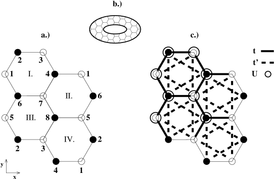
Figure 1: a) The studied system. The hexagons, (sites) are labeled by the index $J=I,II,III,IV$, ($n=1,2,...,8$), and sublattices are indicated by black and white dots. b) The torus-like shape of the system taken with periodic boundary conditions. c) The used Hamiltonian parameters.

The smallest nontrivial system of this type, which retains main properties of the interacting four-electron problem, in the studied situation has $n_{h,h}=n_{h,v}=2$, hence four constituent hexagons with $N_{\Lambda}=8$ different sites, and the corresponding four-electron problem in the singlet case has a 784 dimensional Hilbert space. Being the easiest to treat, we analyze below this case, but the procedure we apply is the same for arbitrary $m_{h}$. The system is presented in Fig.1, while the Hamiltonian $\hat{H}=\hat{H}_{kin}+\hat{H}_{U}$, $\hat{H}_{kin}=\hat{T}_{1}+\hat{T}_{2}$ is given by

$$\hat{T}_{1} = \sum_{\sigma}[t\>\hat{c}^{\dagger}_{1,\sigma}\hat{c}_{2,\sigma}+t\>\hat{c}^{\dagger}_{1,\sigma}\hat{c}_{4,\sigma}+t\>\hat{c}^{\dagger}_{1,\sigma}\hat{c}_{6,\sigma}+t\>\hat{c}^{\dagger}_{2,\sigma}\hat{c}_{3,\sigma}+t\>\hat{c}^{\dagger}_{2,\sigma}\hat{c}_{5,\sigma}+t\>\hat{c}^{\dagger}_{3,\sigma}\hat{c}_{4,\sigma}$$

$$+ t\>\hat{c}^{\dagger}_{3,\sigma}\hat{c}_{8,\sigma}+t\>\hat{c}^{\dagger}_{4,\sigma}\hat{c}_{7,\sigma}+t\>\hat{c}^{\dagger}_{5,\sigma}\hat{c}_{6,\sigma}+t\>\hat{c}^{\dagger}_{5,\sigma}\hat{c}_{8,\sigma}+t\>\hat{c}^{\dagger}_{6,\sigma}\hat{c}_{7,\sigma}+t\>\hat{c}^{\dagger}_{7,\sigma}\hat{c}_{8,\sigma}+H.c.],$$

$$\hat{T}_{2} = \sum_{\sigma}[t^{\prime}_{I}\>\hat{c}^{\dagger}_{1,\sigma}\hat{c}_{3,\sigma}+t^{\prime}_{IV}\>\hat{c}^{\dagger}_{1,\sigma}\hat{c}_{3,\sigma}+t^{\prime}_{II}\>\hat{c}^{\dagger}_{1,\sigma}\hat{c}_{5,\sigma}+t^{\prime}_{IV}\>\hat{c}^{\dagger}_{1,\sigma}\hat{c}_{5,\sigma}+t^{\prime}_{I}\>\hat{c}^{\dagger}_{1,\sigma}\hat{c}_{7,\sigma}+t^{\prime}_{II}\>\hat{c}^{\dagger}_{1,\sigma}\hat{c}_{7,\sigma}$$

$$+ t^{\prime}_{I}\>\hat{c}^{\dagger}_{2,\sigma}\hat{c}_{4,\sigma}+t^{\prime}_{IV}\>\hat{c}^{\dagger}_{2,\sigma}\hat{c}_{4,\sigma}+t^{\prime}_{I}\>\hat{c}^{\dagger}_{2,\sigma}\hat{c}_{6,\sigma}+t^{\prime}_{III}\>\hat{c}^{\dagger}_{2,\sigma}\hat{c}_{6,\sigma}+t^{\prime}_{III}\>\hat{c}^{\dagger}_{2,\sigma}\hat{c}_{8,\sigma}+t^{\prime}_{IV}\>\hat{c}^{\dagger}_{2,\sigma}\hat{c}_{8,\sigma}$$

$$+ t^{\prime}_{III}\>\hat{c}^{\dagger}_{3,\sigma}\hat{c}_{5,\sigma}+t^{\prime}_{IV}\>\hat{c}^{\dagger}_{3,\sigma}\hat{c}_{5,\sigma}+t^{\prime}_{I}\>\hat{c}^{\dagger}_{3,\sigma}\hat{c}_{7,\sigma}+t^{\prime}_{III}\>\hat{c}^{\dagger}_{3,\sigma}\hat{c}_{7,\sigma}+t^{\prime}_{I}\>\hat{c}^{\dagger}_{4,\sigma}\hat{c}_{6,\sigma}+t^{\prime}_{II}\>\hat{c}^{\dagger}_{4,\sigma}\hat{c}_{6,\sigma}$$

$$+ t^{\prime}_{II}\>\hat{c}^{\dagger}_{4,\sigma}\hat{c}_{8,\sigma}+t^{\prime}_{IV}\>\hat{c}^{\dagger}_{4,\sigma}\hat{c}_{8,\sigma}+t^{\prime}_{II}\>\hat{c}^{\dagger}_{5,\sigma}\hat{c}_{7,\sigma}+t^{\prime}_{III}\>\hat{c}^{\dagger}_{5,\sigma}\hat{c}_{7,\sigma}+t^{\prime}_{II}\>\hat{c}^{\dagger}_{6,\sigma}\hat{c}_{8,\sigma}+t^{\prime}_{III}\>\hat{c}^{\dagger}_{6,\sigma}\hat{c}_{8,\sigma}$$

$$+ H.c.],$$

$$\hat{H}_{U} = U\>\hat{n}_{1,\uparrow}\hat{n}_{1,\downarrow}+U\>\hat{n}_{2,\uparrow}\hat{n}_{2,\downarrow}+U\>\hat{n}_{3,\uparrow}\hat{n}_{3,\downarrow}+U\>\hat{n}_{4,\uparrow}\hat{n}_{4,\downarrow}+U\>\hat{n}_{5,\uparrow}\hat{n}_{5,\downarrow}+U\>\hat{n}_{6,\uparrow}\hat{n}_{6,\downarrow}$$ (2)

$$+ U\>\hat{n}_{7,\uparrow}\hat{n}_{7,\downarrow}+U\>\hat{n}_{8,\uparrow}\hat{n}_{8,\downarrow},$$

where $\hat{c}^{\dagger}_{i,\sigma}$ creates an electron with spin projection $\sigma$ on site $i$, $U\geq 0$ characterizes the local Coulomb repulsion, t represents the nearest neighbor hopping matrix element, and $t^{\prime}_{J}=t^{\prime}$ is the next nearest neighbor hopping matrix element inside the hexagon $J=I,II,III,IV$.

III The applied procedure

III.1 The basic strategy of the method

The technique we apply, which has never been used in the study of 2D materials with hexagonal repeat units, has been described in details in Ref.I1 , where it has been successfully utilized in deriving the four-electron ground state for finite 2D Hubbard model on a square lattice. The method works for singlet ground states $|\Psi_{g}\rangle$ provided by an arbitrary even number of electrons, N, whose Hilbert space is ${\cal{H}}$. The procedure itself is based on the identification of a small subspace ${\cal{S}}$ in which the ground state is placed giving rise to the exact, explicit and handable expression of the multielectronic ground state wave function. For example, in case of the 2D square Hubbard system analyzed in Ref. I1 , it was shown that for $N=4$ electrons and $N_{\Lambda}=4\times 4=16$ sites, for which the Hilbert space dimensionality is $Dim({\cal{H}})=14400$, the subspace ${\cal{S}}$ containing $|\Psi_{g}\rangle$ has only the dimension $Dim({\cal{S}})=85$. Hence, in the process of deducing $|\Psi_{g}\rangle$ for the square system in Ref.I1 , working in ${\cal{S}}$ instead of ${\cal{H}}$, one has a 170 times of dimensionality reduction (i.e. two orders of magnitude).

The method constructs the basis vectors of ${\cal{S}}$ based on the following strategy: i) the most interacting particle configuration is part of $|\Psi_{g}\rangle$, and ii) being a translational invariant system, the most interacting particle configuration is equally present with the same weight around all lattice sites. Starting from i),ii), the first base vector $|1\rangle$ of ${\cal{S}}$ is constructed by taking the most interacting particle configuration, translating it to all lattice sites, and adding together all contributions. Once $|1\rangle$ exists, the other base vectors are obtained by the action of the Hamiltonian. This is based on the fact that iii) if a wave vector $|j\rangle$ was such constructed that a particle configuration was translated to all lattice sites and all such obtained contributions were added, than by the action of the Hamiltonian on $|j\rangle$, the obtained new wave vectors $|j^{\prime}\rangle$ have similar properties, but related to different particle configurations. Consequently, $\hat{H}|1\rangle$ produces new $|j^{\prime}\rangle$ vectors, which, if linearly independent, will be considered new base vectors of ${\cal{S}}$, i.e. $|2\rangle$, $|3\rangle$, etc. Similarly, $\hat{H}|2\rangle$, $\hat{H}|3\rangle$, etc. give rise to new base vectors. The procedure is applied till the set of base vectors $\{|1\rangle,|2\rangle,...|N_{\cal{S}}\rangle$ closes in itself.

In order to clarify the used strategy, let us enumerate first the possible particle configurations which can appear in the present case for 4 electrons in a singlet state. One has three possibilities, namely a) two double occupied sites, b) one double occupied site and two electrons with opposite spin on two other different sites, and c) two electrons with spin up and two electrons with spin down, all on different sites. These three possibilities are graphically presented in Fig.2, where a black dot on site ${\bf i}$ represents a double occupancy at the site ${\bf i}$ (see Fig.2.a), a dashed line connecting two different sites ${\bf j}\neq{\bf k}$ represents two electrons, one with spin $\sigma$ at the site ${\bf j}$ and one with spin $-\sigma$ at the site ${\bf k}$, where $\sigma$ is arbitrary (see Fig.2.b), and finally, a full line connecting two different sites ${\bf j}\neq{\bf i}$ represents two electrons placed with the same spin $\sigma$ on the sites ${\bf j}$ and ${\bf i}$, $\sigma$ is arbitrary (see Fig.2.c).

Figure 2: The three possible types of electron states in the system. Black dot at the site ${\bf i}$ means a double occupancy at ${\bf i}$, a dashed line connecting two different sites ${\bf j}\neq{\bf k}$ represents two electrons, one with spin $\sigma$ at the site ${\bf j}$ and one with spin $-\sigma$ at the site ${\bf k}$, where $\sigma$ is arbitrary, and finally, a full line connecting two different sites ${\bf j}\neq{\bf i}$ represents two electrons placed with the same spin $\sigma$ on the sites ${\bf j}$ and ${\bf i}$, $\sigma$ is arbitrary. The plots a), b), and c) represent the three different possibilities that can appear for four electrons in a singlet state.

The mathematical expressions of the normalized wave vectors connected to the graphical presentations in Fig.2 are as follows: Fig.2.a means

$$|\psi_{a}(i,j)\rangle=\big{(}\hat{c}_{i,\uparrow}^{\dagger}\hat{c}_{i,\downarrow}^{\dagger}\big{)}\big{(}\hat{c}_{j,\uparrow}^{\dagger}\hat{c}_{j,\downarrow}^{\dagger}\big{)}|0\rangle,$$ (3)

where $|0\rangle$ represents the bare vacuum, and one has $i\neq j$ and $i<j$.

The mathematical expression connected to Fig.2.b is

$$|\psi_{b}(i;j,k)\rangle=\frac{1}{\sqrt{2}}\big{(}\hat{c}_{i,\uparrow}^{\dagger}\hat{c}_{i,\downarrow}^{\dagger}\big{)}\big{[}\big{(}\hat{c}_{j,\uparrow}^{\dagger}\hat{c}_{k,\downarrow}^{\dagger}\big{)}+\big{(}\hat{c}_{k,\uparrow}^{\dagger}\hat{c}_{j,\downarrow}^{\dagger}\big{)}\big{]}|0\rangle,$$ (4)

where $i\neq j$, $i\neq k$ and $j\neq k$ is required.

Finally, the mathematical meaning of Fig.2.c is given by

$$|\psi_{c}(j,i;l,k)\rangle=\frac{1}{\sqrt{2}}\big{[}\big{(}\hat{c}_{j,\uparrow}^{\dagger}\hat{c}_{i,\uparrow}^{\dagger}\big{)}\big{(}\hat{c}_{l,\downarrow}^{\dagger}\hat{c}_{k,\downarrow}^{\dagger}\big{)}+\big{(}\hat{c}_{j,\downarrow}^{\dagger}\hat{c}_{i,\downarrow}^{\dagger}\big{)}\big{(}\hat{c}_{l,\uparrow}^{\dagger}\hat{c}_{k,\uparrow}^{\dagger}\big{)}\big{]}|0\rangle,$$ (5)

where $i\neq j\neq k\neq l$, together with $j>i$ and $l>k$ must be satisfied.

A given particle configuration is an arbitrary four-electron state contained in one of the vectors presented in Eqs.(3,4,5). The most interacting particle configuration includes two double occupancies placed at nearest neighbor sites.

III.2 The application of the method

The application of the method consists basically of three steps, namely: a) the construction of a starting base vector, b) the application of the Hamiltonian on the starting wave vector and collecting the resultant base vectors describing also resultant configurations placed at different sites and added together, c) further application of the Hamiltonian on the resultant base vectors till the system closes (i.e. new resultant linearly independent vectors no more appear). This happens after a number of steps $N_{\cal{s}}$ (i.e. a number of equations $N_{\cal{s}}$), which is usually orders of magnitude smaller than $Dim({\cal{H}})$. In the present case $N_{\cal{s}}=Dim({\cal{S}})=70$. Below we describe the steps a),b),c) in details.

For the first step, a) we take into consideration the basic starting points of the method. Consequently, one starts with a most interacting configuration ($|\psi_{a}(2,3)\rangle$) and writes it on all (sublattice) sites ($|\psi_{a}(6,7)\rangle,|\psi_{a}(5,8)\rangle,|\psi_{a}(1,4)\rangle$). Since all these configurations must appear with the same weight, we add all these contributions, normalize the sum and obtain the starting base vector of ${\cal{S}}$ as

$$|1\rangle=\frac{1}{2}(|\psi_{a}(2,3)\rangle+|\psi_{a}(6,7)\rangle+|\psi_{a}(5,8)\rangle+|\psi_{a}(1,4)\rangle),$$ (6)

which is represented in graphical form in the first position of Fig.3. Note that one has in the studied sample four sublattice sites, so $|1\rangle$ must have four components.

For the step b) we simply apply the Hamiltonian on $|1\rangle$, obtaining

$$\hat{H}|1\rangle = 2U|1\rangle+2t|8\rangle+2t|10\rangle+4t^{\prime}|17\rangle+4t^{\prime}|18\rangle+4t^{\prime}|22\rangle,$$ (7)

where the new resultant linearly independent base vectors denoted by $|8\rangle,|10\rangle,|17\rangle,|18\rangle,|22\rangle$ can be seen in Figs.3-4. We note that because of the clarity of the presentation, the numbering of the base vectors not follows the order of appearance, but the constituent type. The mathematical expressions corresponding to the graphical representations in Figs.3-8 are simple: for a given vector take every plotted contribution, write them in mathematical form according to the rules described in Eqs.(3,4,5), add all contributions together and finally, normalize the sum.

Now the step c) follows: one applies the Hamiltonian on all new resultant base vectors, obtaining

$$\hat{H}|8\rangle = 2t|1\rangle+2t|4\rangle+U|8\rangle+2t^{\prime}|10\rangle+2t^{\prime}|14\rangle+t|22\rangle+t|25\rangle+2t^{\prime}|27\rangle+2t^{\prime}|28\rangle$$

$$- 2t|37\rangle-2t^{\prime}|42\rangle-2t^{\prime}|43\rangle-2t^{\prime}|47\rangle+t|52\rangle-2t|53\rangle+t|57\rangle-2t^{\prime}|65\rangle,$$

$$\hat{H}|10\rangle = 2t|1\rangle+2t|5\rangle+2t^{\prime}|8\rangle+U|10\rangle+2t^{\prime}|15\rangle+t|22\rangle+t|25\rangle+2t^{\prime}|26\rangle+2t^{\prime}|28\rangle$$

$$- 2t|38\rangle+2t^{\prime}|41\rangle-2t^{\prime}|44\rangle+2t^{\prime}|47\rangle+t|52\rangle+2t|54\rangle+t|57\rangle+2t^{\prime}|66\rangle,$$

$$\hat{H}|17\rangle = 4t^{\prime}|1\rangle+4t^{\prime}|3\rangle+U|17\rangle+2t^{\prime}|18\rangle+2t^{\prime}|19\rangle+2t^{\prime}|20\rangle+2t^{\prime}|22\rangle+t|26\rangle+t|28\rangle$$

$$- 4t^{\prime}|29\rangle+2t^{\prime}|32\rangle+2t^{\prime}|34\rangle+4t^{\prime}|37\rangle+t|41\rangle+t|47\rangle-2t^{\prime}|50\rangle-2t^{\prime}|52\rangle,$$

$$\hat{H}|18\rangle = 4t^{\prime}|1\rangle+4t^{\prime}|2\rangle+2t^{\prime}|17\rangle+U|18\rangle+2t^{\prime}|19\rangle+2t^{\prime}|21\rangle+2t^{\prime}|22\rangle+t|27\rangle+t|28\rangle$$

$$+ 4t^{\prime}|30\rangle+2t^{\prime}|31\rangle+2t^{\prime}|34\rangle+4t^{\prime}|38\rangle-t|42\rangle-t|47\rangle+2t^{\prime}|51\rangle-2t^{\prime}|52\rangle,$$

$$\hat{H}|22\rangle = 4t^{\prime}|1\rangle+4t^{\prime}|7\rangle+t|8\rangle+t|10\rangle+t|14\rangle+t|15\rangle+2t^{\prime}|17\rangle+2t^{\prime}|18\rangle+2t^{\prime}|20\rangle$$ (8)

$$+ 2t^{\prime}|21\rangle+U|22\rangle+2t^{\prime}|31\rangle+2t^{\prime}|32\rangle-4t^{\prime}|33\rangle-t|43\rangle-t|44\rangle-2t^{\prime}|50\rangle$$

$$+ 2t^{\prime}|51\rangle-t|65\rangle+t|66\rangle+4t^{\prime}|68\rangle,$$

where the new resulting base vectors can be seen in Figs.(3-8). Repeating the Hamiltonian action on the newly resulting vectors, the system closes after 70 steps (i.e. after 70 equations). The whole system of equations is presented in Appendix A, and all emerging contributions are depicted in Figs.(3-8). We note that the normalized and orthogonal vectors $|n\rangle$, $n=1,2,...,70$, represent the base vectors of the subspace ${\cal{S}}$.

Figure 3: The structure of the base vectors $|1\rangle-|13\rangle$ of ${\cal{S}}$. The black dot at a given site means a double occupancy at that site, while a dashed line connecting two different sites ${\bf i}\neq{\bf j}$ represents two electrons, one with spin $\sigma$ at the site ${\bf i}$ and one with spin $-\sigma$ at the site ${\bf j}$, where $\sigma$ is arbitrary.

Figure 4: The structure of the base vectors $|14\rangle-|23\rangle$ of ${\cal{S}}$. The meaning of the notations is as in Fig.3.

Figure 5: The structure of the base vectors $|24\rangle-|34\rangle$ of ${\cal{S}}$. Up to the vector $|28\rangle$ the meaning of the notations is as in Fig.3. Starting from the vector $|29\rangle$, the full line connecting two different sites ${\bf i}\neq{\bf j}$ represents two electrons placed with the same spin $\sigma$ on the sites ${\bf i}$ and ${\bf j}$, $\sigma$ being arbitrary.

Figure 6: The structure of the base vectors $|35\rangle-|48\rangle$ of ${\cal{S}}$. The meaning of the notations is as in Figs.(3-5).

Figure 7: The structure of the base vectors $|49\rangle-|62\rangle$ of ${\cal{S}}$. The meaning of the notations is as in Figs.(3-5).

Figure 8: The structure of the base vectors $|63\rangle-|70\rangle$ of ${\cal{S}}$. The meaning of the notations is as in Figs.(3-5).

In order to reproduce the ground state, from Eq.(A1) one expresses the eigenvector providing the smallest energy. The fact that we indeed find the ground state from Appendix A, has been checked by the exact diagonalization in the 784 dimensional full Hilbert space. The obtained ground state energy values, $E_{g}$ (which are the same in both ${\cal{H}}$ and ${\cal{S}}$) are presented below for different $\hat{H}$ parameters in Tables 1-3, where all quantities are expressed in $t$ units.

$t^{\prime}=0$
$U$	$E_{g}$
0.0	-8.000000000000
0.5	-7.826052697604
1.0	-7.675901871093
1.5	-7.545391958586
2.0	-7.431230836069
2.5	-7.330781976775
3.0	-7.241912968838
3.5	-7.162884307355
4.0	-7.092266429238
4.5	-7.028876746763
5.0	-6.971731130272

$t^{\prime}=0.1$
$U$	$E_{g}$
0.0	-7.200000000000
0.5	-7.029096523521
1.0	-6.886663391590
1.5	-6.766883213589
2.0	-6.665278322743
2.5	-6.578374280956
3.0	-6.503455227928
3.5	-6.438383639055
4.0	-6.381465768299
4.5	-6.331350302916
5.0	-6.286951600765

$t^{\prime}=0.5$
$U$	$E_{g}$
0.0	-8.000000000000
0.5	-7.826554868506
1.0	-7.678117036240
1.5	-7.550564402476
2.0	-7.440430706187
2.5	-7.344831780650
3.0	-7.261386257598
3.5	-7.188137025326
4.0	-7.123478675601
4.5	-7.066093843884
5.0	-7.014899323332

Table 1.                            Table 2.                            Table 3.

III.3 Observations relating to the applied procedure

From Eq.(8) it can be observed that the starting vector $|1\rangle$, by the action of the Hamiltonian, reproduces also the vectors $|2\rangle$, $|3\rangle$, which are similar to $|1\rangle$ and can be considered also as of “most interacting configuration” type. Indeed, the whole Eq.(A1) system of equations can be reproduced starting from the vector $|2\rangle$ or vector $|3\rangle$. Note that the impression that these last two vectors have non-parallel (i.e. rotated) contributions is misleading. Indeed, for both $|2\rangle$ and $|3\rangle$, the first two contributions are placed on the outer circumference of the torus, while the second two contributions on the inner circumference of the torus. Consequently, both vectors $|2\rangle$ and $|3\rangle$ are built up only from contributions which are parallel inside the sample.

The study of Figs.(3-8) shows that several possible particle configurations are missing from the ground state (similar property holds also for the square system, see Ref.I1 ). This is because only those configurations are present in $|\Psi_{g}\rangle$ which, by the action of the Hamiltonian, can be connected to the most interacting configuration. That is why, in constructing the base vectors of ${\cal{S}}$ (i.e. Appendix A), we must use a starting vector which describes the most interacting configuration.

We note that in case of the square system described in Ref.I1 , all vectors describing a most-interacting configuration (around a given lattice site, all these can be obtained from each other by a rotation with $\pi/2$), appear always with the same coefficient, so can be added together in a unique starting vector. In our case, however, the vectors $|1\rangle$, $|2\rangle$, $|3\rangle$ do not have this property (i.e. vectors $|1\rangle$, $|2\rangle$, $|3\rangle$ are separated and can not be added together), because the sample we use, does not possess $2\pi/3$ rotational symmetry. Practically this is the reason why one reaches in the studied case only one order of magnitude decrease in reducing $Dim({\cal{H}})$ to $Dim({\cal{S}})$ in the process of deducing the ground state. For clarity, the detailed construction of the components of an arbitrary vector $|i\rangle$ at fixed $i$ in the studied case is presented in Appendix B.

IV Properties of the deduced ground state

By studying the deduced properties, first one notes that the system in Appendix A properly reproduces the ground state, but it is incomplete at the level of excited states. Since several low lying excited states are not provided by Eq.(11), the reduced space ${\cal{S}}$ cannot be used for the study of excitations, or for the estimation of the charge gap.

Turning back to the ground state, with its explicit expression deduced from the reduced ${\cal{S}}$ subspace, several ground state properties of the system can be analyzed.

One often finds continuously increasing singlet ground state energy for Hubbard models at increasing $U$ on finite $U$ domains in one I2 ; I2a ; I2b and two I3 dimensions as well, and even if we know that in 1D, the Bethe Ansatz $E_{g}$ result saturates at $U\to\infty$, see Ref. I4 , we also know that often, the emergence of ferromagnetism at a fixed concentration is associated with the singlet $E_{g}$ increase in function of increasing $U$ I4a .

Consequently, taken into account that the most interacting configuration (i.e. the configuration containing the maximum number of double occupancies dense displaced) enters our ground state, one naively expects that if $U$ increases, the singlet four-particle ground state energy also continuously increases. The result however shows that $E_{g}$ reaches a saturation when $U$ increases (see Fig.9.a), and the system remains in singlet state even at $U\to\infty$. For the 2D case, in exact terms, a such kind of saturation in function of the interaction, in our knowledge, has not been shown yet. The presented property is not connected exclusively to graphene-like systems, since it appears also for 2D square lattice (see Fig.9.b). This last figure has been deduced based on the results I5 published in Ref.I1 .

Figure 9: The ground state energy in function of $U$. a) With hexagonal repeat units, the case presented in Fig.1 at $t^{\prime}/t=0.5$. b) 4x4 square lattice studied in Ref.I1 , where $U$ is in $t$ units.

It turned out that the observed saturation emerges because, even if the most interacting particle configurations (i.e. $|1\rangle,|2\rangle,|3\rangle$) are present in the normalized ground state wave function

$$|\Psi_{g}\rangle=\sum_{i=1}^{70}x_{i}|i\rangle,$$ (9)

the coefficients $x_{i}$ of the basis vectors containing double occupancies strongly decrease with increasing $U$. Indeed, Fig.10 shows the dependence on $U$ of the $|1\rangle$ base vector containing two nearest neighbor double occupancies in a non-degenerate ground state provided by $\hat{H}$ in (2).

Figure 10: The dependence of the $|x_{1}|^{2}$ coefficient of (9) in the ground state of the system with hexagonal repeat units in function of $U$. The ground state is non-degenerate and corresponds to $t^{\prime}/t=-0.6$. The U values are expressed in t units.

Figure 11: The dependence on $U$ of the $|x_{1}|^{2}$ value in case of the square system studied in Ref.I1 (the notation of $|1\rangle$ is taken from Ref.I1 ). The corresponding vector contains two double occupancies on nearest neighbor sites. $U$ is expressed in $t$ units.

As seen, the decrease is strong, and one finds similar behavior also in the square system, see Fig.11. Compairing Figs.10-11, one sees that the emergence probabilities of configurations with two double occupancies in 2D systems with hexagonal and square repeat units, in the presented case, behave similar, and their decrease rate in function of U is also similar expl1 .

Up to this moment the behavior and effects of the interaction in systems with hexagonal and square repeat units seem to be resembling. However, what makes a system with hexagonal repeat units different from the square one, is the emergence of closely placed low lying energy levels which lead to degenerate (or almost degenerate) ground states in extended regions of the phase diagram. This is observed also in other studies relating honeycomb systems I4x ; I4y ; I4z . This situation will be exemplified below (see Figs.12-13) for a ground state $|\Psi_{g}\rangle=|\Psi_{g,1}\rangle$, whose energy $E_{g}=E_{g,1}\leq E_{g,2}$, within the numerical error of the calculation, coincides to the energy $E_{g,2}$ provided by the nearest neighbor level described by $|\Psi_{g,2}\rangle$. Note that for $n=1,2$, the vectors $|\Psi_{g,n}\rangle$ are ortho-normalized. In this case, the emergence probability of different particle configurations in $|\Psi_{g}\rangle$ shows trembling in function of U. For exemplification we present for the start two plots, namely first the $U$ dependence of the $|x_{1}|^{2}$ coefficient in Fig.12, and second, the $U$ dependence of $|x_{8}|^{2}$ coefficient in Fig.13.

Figure 12: The dependence on $U$ of the $|x_{1}|^{2}$ value from Eq.(9) in the case of the system with hexagonal repeat units presented in Fig.1. The corresponding vector contains two double occupancies on nearest neighbor sites. One has $t^{\prime}/t=0.5$, and $U$ is expressed in $t$ units.

Figure 13: The dependence on $U$ of the $|x_{8}|^{2}$ value from Eq.(9) in the case of the system with hexagonal repeat units presented in Fig.1. The corresponding vector contains a double occupancy and two single occupancies on nearest neighbor sites in nearest neighbor position from the double occupied site. One has $t^{\prime}/t=0.5$, and $U$ is expressed in $t$ units.

One notes that the basis vector $|1\rangle$ corresponding to the $|x_{1}|^{2}$ coefficient (see Fig.12) contains two double occupancies placed in neighboring positions, while the basis vector $|8\rangle$ connected to the $|x_{8}|^{2}$ coefficient (see Fig.13) contains only one double occupancy and two single occupancies on nearest neighbor sites in nearest neighbor position from the double occupied site (see Fig.3). In case of Fig.12, the shape of the function at $U\to\infty$ is similar to Fig.13, but now a maximum is reached at $U=2$. The presence of a clear trembling in the $U$ dependence is clearly seen in both cases. For the same conditions, similar behavior is seen in other $|x_{i}|^{2}$ coefficients relating $|i\rangle$ states contained in $|\Psi_{g}\rangle$. In order to exemplify, we present in Figs.14-15 two more cases, the first being related to two double occupancies placed on next nearest neighbor positions (Fig.14), and the second being connected to one double occupancy and two single occupancies on nearest neighbor sites placed in next nearest neighbor position from the double occupied site (Fig.15).

Figure 14: The dependence on $U$ of the $|x_{4}|^{2}$ value from Eq.(9) in the case of the system with hexagonal repeat units presented in Fig.1. The corresponding vector contains two double occupancies placed on next nearest neighbor sites. One has $t^{\prime}/t=0.5$, and $U$ is expressed in $t$ units.

Figure 15: The dependence on $U$ of the $|x_{14}|^{2}$ value from Eq.(9) in the case of the system with hexagonal repeat units presented in Fig.1. The corresponding vector contains one double occupancy and two single occupancies on nearest neighbor sites in next nearest neighbor position from the double occupied site. One has $t^{\prime}/t=0.5$, and $U$ is expressed in $t$ units.

As seen, if the distances between two double occupancies or between a double and a pair of single occupancies in the particle configurations are increased, see Figs.14-15, the trembling character of the behavior and the decrease in function of $U$ at $U\to\infty$ remains, but the value of $|x_{i}|^{2}$ is in the same time strongly diminishes. Similarly to Fig.12, a maximum value can be observed in Fig.14 at $U=1.5$, and in Fig.15 at $U=8.5$. We note that trembling has been observed also at $t^{\prime}=0$.

In order to underline that the trembling is missing in the square case, one presents below three examples in Figs.16-18, namely the case of a double occupancy and two single occupancies on nearest neighbor sites in nearest neighbor position from the double occupied site (Fig.16), the case of two double occupancies placed in third neighbor positions (Fig.17), and finally, the case of one double occupancy and two single occupancies on nearest neighbor sites placed in third neighbor position from the double occupied site (Fig.18).

Figure 16: The dependence on $U$ of the $|x_{2}|^{2}$ value in case of the square system studied in Ref.I1 (the notation of $|2\rangle$ is taken from Ref.I1 ). The corresponding vector contains one double occupancy and two single occupancies on nearest neighbor sites in nearest neighbor position from the double occupied site. $U$ is expressed in $t$ units.

Figure 17: The dependence on $U$ of the $|x_{36}|^{2}$ value in case of the square system studied in Ref.I1 (the notation of $|36\rangle$ is taken from Ref.I1 ). The corresponding vector contains two double occupancies on third neighbor sites. $U$ is expressed in $t$ units.

Figure 18: The dependence on $U$ of the $|x_{66}|^{2}$ value in case of the square system studied in Ref.I1 (the notation of $|66\rangle$ is taken from Ref.I1 ). The corresponding vector contains one double occupancy and two single occupancies on nearest neighbor sites in third neighbor position from the double occupied site. $U$ is expressed in $t$ units.

Figure 19: The $U$ dependence of the $\sum_{n=1}^{2}|x_{1,n}|^{2}=|x_{1,1}|^{2}+|x_{1,2}|^{2}$ sum in the hexagon case, $i=1$ particle configuration and $t^{\prime}/t=0.5$ double degenerate situation. As seen, the trembling in $U$ is missing. The $U$ value is expressed in $t$ units.

Comparing the results deduced for hexagonal repeat units with the case of the square lattice (see Figs.16-18), one observes that the decrease of the $|x_{i}|^{2}$ coefficients in function of $U$ remains, but the trembling is missing, and the maximum disappears.

The trembling (“Zittern” in German language) is known mostly because of the trembling motion (“Zitterbewegung”) of the Dirac electron, namely the trembling of the relativistic electron velocity (hence also the electron position) in function of time Z1 observed by Schrödinger (see for the original derivation Ref.Z2 ). However, it is clear that trembling is not connected to relativity, since can occur also in classical wave propagation phenomena Z3 . In the present case the trembling occurs not in a time dependent phenomenon, but in the $U$ dependence of the emergence probability $|x_{i}|^{2}$ of a particle configuration $i$ described by the state vector $|i\rangle$ present in the ground state.

The trembling appears (as in the Dirac electron case) because of an interference between two states influencing each other in the frame of the concrete event (particle and antiparticle states in Zitterbewegung of Dirac electrons). In the present case the interference is caused by the proximity of two states on the energy scale. In order to check this statement, if one calculates the $\sum_{n=1,2}|x_{1,n}|^{2}$ quantity taking $x_{i,n}$ from $|\Psi_{g,n}\rangle$, $n=1,2$, one finds a continuous (i.e. trembling free) behavior, as observed from Fig.19.

As seen from Figs.16-19, for relatively small U values, an oscillatory contribution is present in trembling (such behavior is present also in the relativistic Zitterbewegung), whose period is close to the $t$ value (note that U is measured in t units), but this is transient, since disappears in $U\to\infty$ limit (see for example the high U region of Fig.14).

We note that if $|\Psi_{g,n}\rangle$, $n=1,2$ describe a rigorously degenerate state, the described trembling behavior remains present in a realistic system. This is because even under the action of an infinitesimally small perturbation, the degeneracy is broken (see for example the case of a short ranged impurity I4x ). Indeed, let us consider $x_{i,n}$, $n=1,2$, the coefficients of the particle configuration $i$ described by the state vector $|i\rangle$ in the degenerate ground state $|\Psi_{g,n}\rangle$. One knows that $x_{i,n}$ are trembling, but as observed from Fig.19, the function $f(U)$ defined by

$$|x_{i,1}|^{2}+|x_{i,2}|^{2}=f(U)$$ (10)

is a continuous non-trembling (i.e. possessing continuous U derivative) function. Then, from the stationary degenerate perturbation theory one knows that the emerging non-degenerate ground state $|\Psi_{g}\rangle$ becomes a linear combination of $|\Psi_{g,n}\rangle$ vectors with fixed prefactors. Hence in $|\Psi_{g}\rangle$, the vector $|i\rangle$ has the coefficient $x_{i}=x_{i,1}+Kx_{i,2}$, where K is fixed, and is explicitly determined by the degenerate perturbation theory. It depends in fact on the matrix elements of the perturbation expressed in terms of the non-perturbed eigenstates belonging to the degenerate level. It can be seen that because of (10), in $|x_{i}|^{2}=|x_{i,1}+Kx_{i,2}|^{2}$ the trembling will be automatically preserved.

The deduced results show that, contrary to square lattices, in 2D systems with hexagonal repeat units strong variations in the system are possible to appear following small, even infinitesimal modifications in the value of the interaction. Given by this property, the interaction dependent behavior of a honeycomb system as graphene could substantially differ from the behavior of a square lattice, even for concentrations which place far away the Fermi level from the Dirac points. Such in principle differences in the behavior could cause controversies as encountered in Refs.[Intr18 ; Intr19 ; Intr20 ].

One notes that the presented technique can be applied also in the presence of non-local interactions. On this line we expect that density-density type of non-local interactions essentially will not modify the observed properties. Furthermore, in the presence of local interactions, the brick-wall lattice (see for example Ref.[Z4 ]) at $t^{\prime}=0$ has the spectrum of the honeycomb lattice. Taking next-nearest neighbor hoppings into account, differences appear relative to the honeycomb case, because $t^{\prime}_{1},t^{\prime}_{2}$ must be defined instead of a single next-nearest neighbor $t^{\prime}$ hopping term. However, we do not expect that this difference will alter in main aspects the behavior described in this paper.

V Summary and discussions

We deduced the exact interacting four particle ground state of a 2D finite sample described by a Hubbard type of model and build up from hexagon repeat units. The ground state is obtained exactly from a restricted space ${\cal{S}}$ with dimensionality much smaller than the dimension of the full Hilbert space ${\cal{H}}$ of the problem, $D_{\cal{S}}=Dim({\cal{S}})<<Dim({\cal{H}})=D_{\cal{H}}$. The used technique begins from a starting wave vector $|1\rangle$ containing the most interacting particle configuration (i.e. two nearest neighbor double occupancies) translated to all sublattice sites and added). The application of the Hamiltonian ($\hat{H}$) on $|1\rangle$ leads to further vectors $|i\rangle$ with similar properties, i.e. a local particle configuration translated to different sites and added. Taken together, the $\hat{H}|i\rangle=\sum_{j}\alpha_{j,i}|j\rangle$ equalities build up a closed system of linear equations for $i\leq D_{\cal{S}}<<D_{\cal{H}}$, whose minimum energy solution represents the ground state. We note that the ground state was always found a non-magnetic singlet state.

With the exact ground state in hands, different properties of the system have been analyzed. We have found that contrary to expectations, the singlet ground state energy saturates in the limit of infinite on-site Coulomb repulsion, and the emergence probability of different particle configurations in the ground state presents trembling (“Zittern”) in function of $U$, this property being absent in the case of a square lattice. The trembling behavior has been shown to appear because of the interference between states placed in the proximity of each other on the energy scale. It can lead to strong modifications of the system properties caused by small variations of the interaction strength, and can be the source of the differences in the interaction dependent behavior of square and honeycomb 2D systems.

VI Acknowledgments

Z.G. kindly acknowledges financial support provided by Alexander von Humboldt Foundation, OTKA-K-100288 (Hungarian Research Funds for Basic Research), and TAMOP 4.2.2/A-11/1/KONV-2012-0036 (co-financed by EU and European Social Fund).

Appendix A The system of equations providing the ground state in the 70 dimensional subspace ${\cal{S}}$.

$$\hat{H}|1\rangle = 2U|1\rangle+2t|8\rangle+2t|10\rangle+4t^{\prime}|17\rangle+4t^{\prime}|18\rangle+4t^{\prime}|22\rangle,$$

$$\hat{H}|2\rangle = 2U|2\rangle+2t|11\rangle+2t|13\rangle+4t^{\prime}|18\rangle+4t^{\prime}|19\rangle+4t^{\prime}|21\rangle,$$

$$\hat{H}|3\rangle = 2U|3\rangle+2t|9\rangle+2t|12\rangle+4t^{\prime}|17\rangle+4t^{\prime}|19\rangle+4t^{\prime}|20\rangle,$$

$$\hat{H}|4\rangle = 2U|4\rangle+2t|8\rangle+2t|12\rangle+2t|14\rangle+4t^{\prime}|23\rangle+4t^{\prime}|25\rangle,$$

$$\hat{H}|5\rangle = 2U|5\rangle+2t|10\rangle+2t|13\rangle+2t|15\rangle+4t^{\prime}|24\rangle+4t^{\prime}|25\rangle,$$

$$\hat{H}|6\rangle = 2U|6\rangle+2t|9\rangle+2t|11\rangle+2t|16\rangle+4t^{\prime}|23\rangle+4t^{\prime}|24\rangle,$$

$$\hat{H}|7\rangle = 2U|7\rangle+2t|14\rangle+2t|15\rangle+2t|16\rangle+4t^{\prime}|20\rangle+4t^{\prime}|21\rangle+4t^{\prime}|22\rangle,$$

$$\hat{H}|8\rangle = 2t|1\rangle+2t|4\rangle+U|8\rangle+2t^{\prime}|10\rangle+2t^{\prime}|14\rangle+t|22\rangle+t|25\rangle+2t^{\prime}|27\rangle+2t^{\prime}|28\rangle$$

$$- 2t|37\rangle-2t^{\prime}|42\rangle-2t^{\prime}|43\rangle-2t^{\prime}|47\rangle+t|52\rangle-2t|53\rangle+t|57\rangle-2t^{\prime}|65\rangle,$$

$$\hat{H}|9\rangle = 2t|3\rangle+2t|6\rangle+U|9\rangle+2t^{\prime}|12\rangle+2t^{\prime}|16\rangle+t|20\rangle+t|23\rangle+2t^{\prime}|26\rangle+2t^{\prime}|28\rangle$$

$$+ 2t|35\rangle+2t^{\prime}|41\rangle+2t^{\prime}|47\rangle-2t^{\prime}|48\rangle+t|50\rangle+t|55\rangle+2t|63\rangle+2t^{\prime}|67\rangle,$$

$$\hat{H}|10\rangle = 2t|1\rangle+2t|5\rangle+2t^{\prime}|8\rangle+U|10\rangle+2t^{\prime}|15\rangle+t|22\rangle+t|25\rangle+2t^{\prime}|26\rangle+2t^{\prime}|28\rangle$$

$$- 2t|38\rangle+2t^{\prime}|41\rangle-2t^{\prime}|44\rangle+2t^{\prime}|47\rangle+t|52\rangle+2t|54\rangle+t|57\rangle+2t^{\prime}|66\rangle,$$

$$\hat{H}|11\rangle = 2t|2\rangle+2t|6\rangle+U|11\rangle+2t^{\prime}|13\rangle+2t^{\prime}|16\rangle+t|21\rangle+t|24\rangle+2t^{\prime}|27\rangle+2t^{\prime}|28\rangle$$

$$- 2t|36\rangle-2t^{\prime}|42\rangle-2t^{\prime}|47\rangle-2t^{\prime}|49\rangle-t|51\rangle-t|56\rangle-2t|63\rangle-2t^{\prime}|67\rangle,$$

$$\hat{H}|12\rangle = 2t|3\rangle+2t|4\rangle+2t^{\prime}|9\rangle+U|12\rangle+2t^{\prime}|14\rangle+t|20\rangle+t|23\rangle+2t^{\prime}|26\rangle+2t^{\prime}|27\rangle$$

$$+ 2t|29\rangle-2t^{\prime}|41\rangle+2t^{\prime}|42\rangle+2t^{\prime}|45\rangle+t|50\rangle+2t|53\rangle+t|55\rangle+2t^{\prime}|65\rangle,$$

$$\hat{H}|13\rangle = 2t|2\rangle+2t|5\rangle+2t^{\prime}|11\rangle+U|13\rangle+2t^{\prime}|15\rangle+t|21\rangle+t|24\rangle+2t^{\prime}|26\rangle+2t^{\prime}|27\rangle$$

$$- 2t|30\rangle-2t^{\prime}|41\rangle+2t^{\prime}|42\rangle-2t^{\prime}|46\rangle-t|51\rangle-2t|54\rangle-t|56\rangle-2t^{\prime}|66\rangle,$$

$$\hat{H}|14\rangle = 2t|4\rangle+2t|7\rangle+2t^{\prime}|8\rangle+2t^{\prime}|12\rangle+U|14\rangle+2t^{\prime}|15\rangle+2t^{\prime}|16\rangle+t|20\rangle+t|22\rangle$$

$$+ t|23\rangle+t|25\rangle-2t^{\prime}|44\rangle-2t^{\prime}|48\rangle+t|50\rangle+t|52\rangle+t|55\rangle+t|57\rangle-2t|61\rangle$$

$$+ 2t^{\prime}|66\rangle+2t^{\prime}|67\rangle+2t|69\rangle,$$

$$\hat{H}|15\rangle = 2t|5\rangle+2t|7\rangle+2t^{\prime}|10\rangle+2t^{\prime}|13\rangle+2t^{\prime}|14\rangle+U|15\rangle+2t^{\prime}|16\rangle+t|21\rangle+t|22\rangle$$

$$+ t|24\rangle+t|25\rangle-2t^{\prime}|43\rangle-2t^{\prime}|49\rangle-t|51\rangle+t|52\rangle-t|56\rangle+t|57\rangle-2t|62\rangle$$

$$- 2t^{\prime}|65\rangle-2t^{\prime}|67\rangle-2t|70\rangle,$$

$$\hat{H}|16\rangle = 2t|6\rangle+2t|7\rangle+2t^{\prime}|9\rangle+2t^{\prime}|11\rangle+2t^{\prime}|14\rangle+2t^{\prime}|15\rangle+U|16\rangle+t|20\rangle+t|21\rangle$$

$$+ t|23\rangle+t|24\rangle+2t^{\prime}|45\rangle-2t^{\prime}|46\rangle+t|50\rangle-t|51\rangle+t|55\rangle-t|56\rangle-2t|58\rangle$$

$$+ 2t^{\prime}|65\rangle-2t^{\prime}|66\rangle-2t|68\rangle,$$

$$\hat{H}|17\rangle = 4t^{\prime}|1\rangle+4t^{\prime}|3\rangle+U|17\rangle+2t^{\prime}|18\rangle+2t^{\prime}|19\rangle+2t^{\prime}|20\rangle+2t^{\prime}|22\rangle+t|26\rangle+t|28\rangle$$

$$- 4t^{\prime}|29\rangle+2t^{\prime}|32\rangle+2t^{\prime}|34\rangle+4t^{\prime}|37\rangle+t|41\rangle+t|47\rangle-2t^{\prime}|50\rangle-2t^{\prime}|52\rangle,$$

$$\hat{H}|18\rangle = 4t^{\prime}|1\rangle+4t^{\prime}|2\rangle+2t^{\prime}|17\rangle+U|18\rangle+2t^{\prime}|19\rangle+2t^{\prime}|21\rangle+2t^{\prime}|22\rangle+t|27\rangle+t|28\rangle$$

$$+ 4t^{\prime}|30\rangle+2t^{\prime}|31\rangle+2t^{\prime}|34\rangle+4t^{\prime}|38\rangle-t|42\rangle-t|47\rangle+2t^{\prime}|51\rangle-2t^{\prime}|52\rangle,$$

$$\hat{H}|19\rangle = 4t^{\prime}|2\rangle+4t^{\prime}|3\rangle+2t^{\prime}|17\rangle+2t^{\prime}|18\rangle+U|19\rangle+2t^{\prime}|20\rangle+2t^{\prime}|21\rangle+t|26\rangle+t|27\rangle$$

$$+ 2t^{\prime}|31\rangle+2t^{\prime}|32\rangle-4t^{\prime}|35\rangle+4t^{\prime}|36\rangle-t|41\rangle+t|42\rangle-2t^{\prime}|50\rangle+2t^{\prime}|51\rangle,$$

$$\hat{H}|20\rangle = 4t^{\prime}|3\rangle+4t^{\prime}|7\rangle+t|9\rangle+t|12\rangle+t|14\rangle+t|16\rangle+2t^{\prime}|17\rangle+2t^{\prime}|19\rangle+U|20\rangle$$

$$+ 2t^{\prime}|21\rangle+2t^{\prime}|22\rangle+2t^{\prime}|31\rangle+2t^{\prime}|34\rangle-4t^{\prime}|39\rangle+t|45\rangle-t|48\rangle+2t^{\prime}|51\rangle$$

$$- 2t^{\prime}|52\rangle+t|65\rangle+t|67\rangle+4t^{\prime}|70\rangle,$$

$$\hat{H}|21\rangle = 4t^{\prime}|2\rangle+4t^{\prime}|7\rangle+t|11\rangle+t|13\rangle+t|15\rangle+t|16\rangle+2t^{\prime}|18\rangle+2t^{\prime}|19\rangle+2t^{\prime}|20\rangle$$

$$+ U|21\rangle+2t^{\prime}|22\rangle+2t^{\prime}|32\rangle+2t^{\prime}|34\rangle-4t^{\prime}|40\rangle-t|46\rangle-t|49\rangle-2t^{\prime}|50\rangle$$

$$- 2t^{\prime}|52\rangle-t|66\rangle-t|67\rangle-4t^{\prime}|69\rangle,$$

$$\hat{H}|22\rangle = 4t^{\prime}|1\rangle+4t^{\prime}|7\rangle+t|8\rangle+t|10\rangle+t|14\rangle+t|15\rangle+2t^{\prime}|17\rangle+2t^{\prime}|18\rangle+2t^{\prime}|20\rangle$$

$$+ 2t^{\prime}|21\rangle+U|22\rangle+2t^{\prime}|31\rangle+2t^{\prime}|32\rangle-4t^{\prime}|33\rangle-t|43\rangle-t|44\rangle-2t^{\prime}|50\rangle$$

$$+ 2t^{\prime}|51\rangle-t|65\rangle+t|66\rangle+4t^{\prime}|68\rangle,$$

$$\hat{H}|23\rangle = 4t^{\prime}|4\rangle+4t^{\prime}|6\rangle+t|9\rangle+t|12\rangle+t|14\rangle+t|16\rangle+U|23\rangle+t|27\rangle+t|28\rangle$$

$$- t|42\rangle+t|45\rangle-t|47\rangle-t|48\rangle+4t^{\prime}|59\rangle+4t^{\prime}|64\rangle+t|65\rangle+t|67\rangle,$$

$$\hat{H}|24\rangle = 4t^{\prime}|5\rangle+4t^{\prime}|6\rangle+t|11\rangle+t|13\rangle+t|15\rangle+t|16\rangle+U|24\rangle+t|26\rangle+t|28\rangle$$

$$+ t|41\rangle-t|46\rangle+t|47\rangle-t|49\rangle-4t^{\prime}|60\rangle-4t^{\prime}|64\rangle-t|66\rangle-t|67\rangle,$$

$$\hat{H}|25\rangle = 4t^{\prime}|4\rangle+4t^{\prime}|5\rangle+t|8\rangle+t|10\rangle+t|14\rangle+t|15\rangle+U|25\rangle+t|26\rangle+t|27\rangle$$

$$- t|41\rangle+t|42\rangle-t|43\rangle-t|44\rangle-4t^{\prime}|59\rangle+4t^{\prime}|60\rangle-t|65\rangle+t|66\rangle,$$

$$\hat{H}|26\rangle = 2t^{\prime}|9\rangle+2t^{\prime}|10\rangle+2t^{\prime}|12\rangle+2t^{\prime}|13\rangle+t|17\rangle+t|19\rangle+t|24\rangle+t|25\rangle+U|26\rangle$$

$$- t|31\rangle-t|34\rangle+2t^{\prime}|43\rangle-2t^{\prime}|45\rangle+2t^{\prime}|48\rangle+2t^{\prime}|49\rangle+t|56\rangle-t|57\rangle,$$

$$\hat{H}|27\rangle = 2t^{\prime}|8\rangle+2t^{\prime}|11\rangle+2t^{\prime}|12\rangle+2t^{\prime}|13\rangle+t|18\rangle+t|19\rangle+t|23\rangle+t|25\rangle+U|27\rangle$$

$$- t|32\rangle-t|34\rangle+2t^{\prime}|44\rangle+2t^{\prime}|46\rangle+2t^{\prime}|48\rangle+2t^{\prime}|49\rangle-t|55\rangle-t|57\rangle,$$

$$\hat{H}|28\rangle = 2t^{\prime}|8\rangle+2t^{\prime}|9\rangle+2t^{\prime}|10\rangle+2t^{\prime}|11\rangle+t|17\rangle+t|18\rangle+t|23\rangle+t|24\rangle+U|28\rangle$$

$$- t|31\rangle-t|32\rangle+2t^{\prime}|43\rangle+2t^{\prime}|44\rangle-2t^{\prime}|45\rangle+2t^{\prime}|46\rangle-t|55\rangle+t|56\rangle,$$

$$\hat{H}|29\rangle = 2t|12\rangle-4t^{\prime}|17\rangle-4t^{\prime}|34\rangle+2t|45\rangle+4t^{\prime}|50\rangle,$$

$$\hat{H}|30\rangle = -2t|13\rangle+4t^{\prime}|18\rangle+4t^{\prime}|34\rangle+2t|46\rangle+4t^{\prime}|51\rangle,$$

$$\hat{H}|31\rangle = 2t^{\prime}|18\rangle+2t^{\prime}|19\rangle+2t^{\prime}|20\rangle+2t^{\prime}|22\rangle-t|26\rangle-t|28\rangle+2t^{\prime}|32\rangle-4t^{\prime}|33\rangle$$

$$+ 2t^{\prime}|34\rangle-4t^{\prime}|35\rangle+4t^{\prime}|38\rangle-4t^{\prime}|39\rangle-t|41\rangle-t|47\rangle-2t^{\prime}|50\rangle-2t^{\prime}|52\rangle,$$

$$\hat{H}|32\rangle = 2t^{\prime}|17\rangle+2t^{\prime}|19\rangle+2t^{\prime}|21\rangle+2t^{\prime}|22\rangle-t|27\rangle-t|28\rangle+2t^{\prime}|31\rangle-4t^{\prime}|33\rangle$$

$$+ 2t^{\prime}|34\rangle+4t^{\prime}|36\rangle+4t^{\prime}|37\rangle-4t^{\prime}|40\rangle+t|42\rangle+t|47\rangle+2t^{\prime}|51\rangle-2t^{\prime}|52\rangle,$$

$$\hat{H}|33\rangle = -4t^{\prime}|22\rangle-4t^{\prime}|31\rangle-4t^{\prime}|32\rangle+2t|43\rangle+2t|44\rangle,$$

$$\hat{H}|34\rangle = 2t^{\prime}|17\rangle+2t^{\prime}|18\rangle+2t^{\prime}|20\rangle+2t^{\prime}|21\rangle-t|26\rangle-t|27\rangle-4t^{\prime}|29\rangle+4t^{\prime}|30\rangle$$

$$+ 2t^{\prime}|31\rangle+2t^{\prime}|32\rangle-4t^{\prime}|39\rangle-4t^{\prime}|40\rangle+t|41\rangle-t|42\rangle-2t^{\prime}|50\rangle+2t^{\prime}|51\rangle,$$

$$\hat{H}|35\rangle = 2t|9\rangle-4t^{\prime}|19\rangle-4t^{\prime}|31\rangle-2t|48\rangle+4t^{\prime}|50\rangle,$$

$$\hat{H}|36\rangle = -2t|11\rangle+4t^{\prime}|19\rangle+4t^{\prime}|32\rangle+2t|49\rangle+4t^{\prime}|51\rangle,$$

$$\hat{H}|37\rangle = -2t|8\rangle+4t^{\prime}|17\rangle+4t^{\prime}|32\rangle+2t|43\rangle-4t^{\prime}|52\rangle,$$

$$\hat{H}|38\rangle = -2t|10\rangle+4t^{\prime}|18\rangle+4t^{\prime}|31\rangle+2t|44\rangle-4t^{\prime}|52\rangle,$$

$$\hat{H}|39\rangle = -4t^{\prime}|20\rangle-4t^{\prime}|31\rangle-4t^{\prime}|34\rangle-2t|45\rangle+2t|48\rangle,$$

$$\hat{H}|40\rangle = -4t^{\prime}|21\rangle-4t^{\prime}|32\rangle-4t^{\prime}|34\rangle+2t|46\rangle+2t|49\rangle,$$

$$\hat{H}|41\rangle = 2t^{\prime}|9\rangle+2t^{\prime}|10\rangle-2t^{\prime}|12\rangle-2t^{\prime}|13\rangle+t|17\rangle-t|19\rangle+t|24\rangle-t|25\rangle$$

$$- t|31\rangle+t|34\rangle+2t^{\prime}|43\rangle-2t^{\prime}|45\rangle-2t^{\prime}|48\rangle-2t^{\prime}|49\rangle+t|56\rangle+t|57\rangle,$$

$$\hat{H}|42\rangle = -2t^{\prime}|8\rangle-2t^{\prime}|11\rangle+2t^{\prime}|12\rangle+2t^{\prime}|13\rangle-t|18\rangle+t|19\rangle-t|23\rangle+t|25\rangle$$

$$+ t|32\rangle-t|34\rangle-2t^{\prime}|44\rangle-2t^{\prime}|46\rangle+2t^{\prime}|48\rangle+2t^{\prime}|49\rangle+t|55\rangle-t|57\rangle,$$

$$\hat{H}|43\rangle = -2t^{\prime}|8\rangle-2t^{\prime}|15\rangle-t|22\rangle-t|25\rangle+2t^{\prime}|26\rangle+2t^{\prime}|28\rangle+2t|33\rangle+2t|37\rangle$$

$$+ 2t^{\prime}|41\rangle+2t^{\prime}|44\rangle+2t^{\prime}|47\rangle-t|52\rangle-t|57\rangle-2t|60\rangle+2t|62\rangle-2t^{\prime}|66\rangle,$$

$$\hat{H}|44\rangle = -2t^{\prime}|10\rangle-2t^{\prime}|14\rangle-t|22\rangle-t|25\rangle+2t^{\prime}|27\rangle+2t^{\prime}|28\rangle+2t|33\rangle+2t|38\rangle$$

$$- 2t^{\prime}|42\rangle+2t^{\prime}|43\rangle-2t^{\prime}|47\rangle-t|52\rangle-t|57\rangle+2t|59\rangle+2t|61\rangle+2t^{\prime}|65\rangle,$$

$$\hat{H}|45\rangle = 2t^{\prime}|12\rangle+2t^{\prime}|16\rangle+t|20\rangle+t|23\rangle-2t^{\prime}|26\rangle-2t^{\prime}|28\rangle+2t|29\rangle-2t|39\rangle$$

$$- 2t^{\prime}|41\rangle-2t^{\prime}|47\rangle-2t^{\prime}|48\rangle+t|50\rangle+t|55\rangle-2t|58\rangle+2t|64\rangle+2t^{\prime}|67\rangle,$$

$$\hat{H}|46\rangle = -2t^{\prime}|13\rangle-2t^{\prime}|16\rangle-t|21\rangle-t|24\rangle+2t^{\prime}|27\rangle+2t^{\prime}|28\rangle+2t|30\rangle+2t|40\rangle$$

$$- 2t^{\prime}|42\rangle-2t^{\prime}|47\rangle+2t^{\prime}|49\rangle+t|51\rangle+t|56\rangle+2t|58\rangle+2t|64\rangle+2t^{\prime}|67\rangle,$$

$$\hat{H}|47\rangle = -2t^{\prime}|8\rangle+2t^{\prime}|9\rangle+2t^{\prime}|10\rangle-2t^{\prime}|11\rangle+t|17\rangle-t|18\rangle-t|23\rangle+t|24\rangle$$

$$- t|31\rangle+t|32\rangle+2t^{\prime}|43\rangle-2t^{\prime}|44\rangle-2t^{\prime}|45\rangle-2t^{\prime}|46\rangle+t|55\rangle+t|56\rangle,$$

$$\hat{H}|48\rangle = -2t^{\prime}|9\rangle-2t^{\prime}|14\rangle-t|20\rangle-t|23\rangle+2t^{\prime}|26\rangle+2t^{\prime}|27\rangle-2t|35\rangle+2t|39\rangle$$

$$- 2t^{\prime}|41\rangle+2t^{\prime}|42\rangle-2t^{\prime}|45\rangle-t|50\rangle-t|55\rangle-2t|59\rangle+2t|61\rangle-2t^{\prime}|65\rangle,$$

$$\hat{H}|49\rangle = -2t^{\prime}|11\rangle-2t^{\prime}|15\rangle-t|21\rangle-t|24\rangle+2t^{\prime}|26\rangle+2t^{\prime}|27\rangle+2t|36\rangle+2t|40\rangle$$

$$- 2t^{\prime}|41\rangle+2t^{\prime}|42\rangle+2t^{\prime}|46\rangle+t|51\rangle+t|56\rangle+2t|60\rangle+2t|62\rangle+2t^{\prime}|66\rangle,$$

$$\hat{H}|50\rangle = t|9\rangle+t|12\rangle+t|14\rangle+t|16\rangle-2t^{\prime}|17\rangle-2t^{\prime}|19\rangle-2t^{\prime}|21\rangle-2t^{\prime}|22\rangle+4t^{\prime}|29\rangle$$

$$- 2t^{\prime}|31\rangle-2t^{\prime}|34\rangle+4t^{\prime}|35\rangle+t|45\rangle-t|48\rangle-2t^{\prime}|51\rangle+2t^{\prime}|52\rangle+t|65\rangle+t|67\rangle$$

$$- 4t^{\prime}|68\rangle+4t^{\prime}|69\rangle,$$

$$\hat{H}|51\rangle = -t|11\rangle-t|13\rangle-t|15\rangle-t|16\rangle+2t^{\prime}|18\rangle+2t^{\prime}|19\rangle+2t^{\prime}|20\rangle+2t^{\prime}|22\rangle+4t^{\prime}|30\rangle$$

$$+ 2t^{\prime}|32\rangle+2t^{\prime}|34\rangle+4t^{\prime}|36\rangle+t|46\rangle+t|49\rangle-2t^{\prime}|50\rangle-2t^{\prime}|52\rangle+t|66\rangle+t|67\rangle$$

$$+ 4t^{\prime}|68\rangle+4t^{\prime}|70\rangle,$$

$$\hat{H}|52\rangle = t|8\rangle+t|10\rangle+t|14\rangle+t|15\rangle-2t^{\prime}|17\rangle-2t^{\prime}|18\rangle-2t^{\prime}|20\rangle-2t^{\prime}|21\rangle-2t^{\prime}|31\rangle$$

$$- 2t^{\prime}|32\rangle-4t^{\prime}|37\rangle-4t^{\prime}|38\rangle-t|43\rangle-t|44\rangle+2t^{\prime}|50\rangle-2t^{\prime}|51\rangle-t|65\rangle+t|66\rangle$$

$$+ 4t^{\prime}|69\rangle-4t^{\prime}|70\rangle,$$

$$\hat{H}|53\rangle = -2t|8\rangle+2t|12\rangle+4t^{\prime}|55\rangle-4t^{\prime}|57\rangle+2t|65\rangle,$$

$$\hat{H}|54\rangle = 2t|10\rangle-2t|13\rangle+4t^{\prime}|56\rangle+4t^{\prime}|57\rangle+2t|66\rangle,$$

$$\hat{H}|55\rangle = t|9\rangle+t|12\rangle+t|14\rangle+t|16\rangle-t|27\rangle-t|28\rangle+t|42\rangle+t|45\rangle+t|47\rangle$$

$$- t|48\rangle+4t^{\prime}|53\rangle-4t^{\prime}|58\rangle-4t^{\prime}|61\rangle+4t^{\prime}|63\rangle+t|65\rangle+t|67\rangle,$$

$$\hat{H}|56\rangle = -t|11\rangle-t|13\rangle-t|15\rangle-t|16\rangle+t|26\rangle+t|28\rangle+t|41\rangle+t|46\rangle+t|47\rangle$$

$$+ t|49\rangle+4t^{\prime}|54\rangle+4t^{\prime}|58\rangle+4t^{\prime}|62\rangle+4t^{\prime}|63\rangle+t|66\rangle+t|67\rangle,$$

$$\hat{H}|57\rangle = t|8\rangle+t|10\rangle+t|14\rangle+t|15\rangle-t|26\rangle-t|27\rangle+t|41\rangle-t|42\rangle-t|43\rangle$$

$$- t|44\rangle-4t^{\prime}|53\rangle+4t^{\prime}|54\rangle-4t^{\prime}|61\rangle-4t^{\prime}|62\rangle-t|65\rangle+t|66\rangle,$$

$$\hat{H}|58\rangle = -2t|16\rangle-2t|45\rangle+2t|46\rangle-4t^{\prime}|55\rangle+4t^{\prime}|56\rangle,$$

$$\hat{H}|59\rangle = 4t^{\prime}|23\rangle-4t^{\prime}|25\rangle+2t|44\rangle-2t|48\rangle+2t|65\rangle,$$

$$\hat{H}|60\rangle = -4t^{\prime}|24\rangle+4t^{\prime}|25\rangle-2t|43\rangle+2t|49\rangle+2t|66\rangle,$$

$$\hat{H}|61\rangle = -2t|14\rangle+2t|44\rangle+2t|48\rangle-4t^{\prime}|55\rangle-4t^{\prime}|57\rangle,$$

$$\hat{H}|62\rangle = -2t|15\rangle+2t|43\rangle+2t|49\rangle+4t^{\prime}|56\rangle-4t^{\prime}|57\rangle,$$

$$\hat{H}|63\rangle = 2t|9\rangle-2t|11\rangle+4t^{\prime}|55\rangle+4t^{\prime}|56\rangle+2t|67\rangle,$$

$$\hat{H}|64\rangle = 4t^{\prime}|23\rangle-4t^{\prime}|24\rangle+2t|45\rangle+2t|46\rangle+2t|67\rangle,$$

$$\hat{H}|65\rangle = -2t^{\prime}|8\rangle+2t^{\prime}|12\rangle-2t^{\prime}|15\rangle+2t^{\prime}|16\rangle+t|20\rangle-t|22\rangle+t|23\rangle-t|25\rangle+2t^{\prime}|44\rangle$$

$$- 2t^{\prime}|48\rangle+t|50\rangle-t|52\rangle+2t|53\rangle+t|55\rangle-t|57\rangle+2t|59\rangle-2t^{\prime}|66\rangle+2t^{\prime}|67\rangle$$

$$- 2t|68\rangle+2t|70\rangle,$$

$$\hat{H}|66\rangle = 2t^{\prime}|10\rangle-2t^{\prime}|13\rangle+2t^{\prime}|14\rangle-2t^{\prime}|16\rangle-t|21\rangle+t|22\rangle-t|24\rangle+t|25\rangle-2t^{\prime}|43\rangle$$

$$+ 2t^{\prime}|49\rangle+t|51\rangle+t|52\rangle+2t|54\rangle+t|56\rangle+t|57\rangle+2t|60\rangle-2t^{\prime}|65\rangle+2t^{\prime}|67\rangle$$

$$+ 2t|68\rangle+2t|69\rangle,$$

$$\hat{H}|67\rangle = 2t^{\prime}|9\rangle-2t^{\prime}|11\rangle+2t^{\prime}|14\rangle-2t^{\prime}|15\rangle+t|20\rangle-t|21\rangle+t|23\rangle-t|24\rangle+2t^{\prime}|45\rangle$$

$$+ 2t^{\prime}|46\rangle+t|50\rangle+t|51\rangle+t|55\rangle+t|56\rangle+2t|63\rangle+2t|64\rangle+2t^{\prime}|65\rangle+2t^{\prime}|66\rangle$$

$$+ 2t|69\rangle+2t|70\rangle,$$

$$\hat{H}|68\rangle = -2t|16\rangle+4t^{\prime}|22\rangle-4t^{\prime}|50\rangle+4t^{\prime}|51\rangle-2t|65\rangle+2t|66\rangle,$$

$$\hat{H}|69\rangle = 2t|14\rangle-4t^{\prime}|21\rangle+4t^{\prime}|50\rangle+4t^{\prime}|52\rangle+2t|66\rangle+2t|67\rangle,$$

$$\hat{H}|70\rangle = -2t|15\rangle+4t^{\prime}|20\rangle+4t^{\prime}|51\rangle-4t^{\prime}|52\rangle+2t|65\rangle+2t|67\rangle.$$ (11)

Appendix B The construction of the wave vectors $|i\rangle$

In this appendix we present the construction of the wave vectors $|i\rangle$ presented in Figs.3-8 and used in Eq.(11). Each vector $|i\rangle$ has maximum 8 components and can be written as

$$|i\rangle=N_{i}\sum_{m=1}^{8}|i_{m}\rangle,$$ (12)

where $N_{i}$ is a numerical factor preserving the normalization to unity, and $|i_{m}\rangle$ represents the mathematical expression based on Eqs.(3,4,5) of the plotted particle configurations ${\cal{C}}_{i,m}$, $m=1,2,..8$ presented in the row $|i\rangle$ of Figs.3-8. If the row $|i\rangle$ from Figs.3-8 contains less than 8 contributions, that means that some of $|i_{m}\rangle$ components taken at fixed $i$ coincide. Note that in a fixed row $|i\rangle$ of Figs.3-8, different contributions are plotted in the order of increasing $m$ index.

If at fixed $i$, the $m=1$ local particle configuration ${\cal{C}}_{i,1}$ is known (this is plotted in the first position of the row $|i\rangle$), all local particle configurations ${\cal{C}}_{i,m}$, $m=2,3,..8$ can be deduced from it as follows: One takes the four axes defined by $\gamma=x,y_{1},y_{2},a$ in Fig.20, and define the transformations: $Tr(\gamma\neq x)$ as the translation (in the axis direction) along the axis $\gamma\neq x$ by vector ${\bf b}$ whose length is equal to the distance to the nearest neighbor along the axis; and $R(\gamma\neq a)$ as a rotation with $\pi$ along the axis $\gamma$.

Figure 20: The axes $\gamma=x,y_{1},y_{2},a$ of the transformations leading to the components $|i_{m}\rangle$ at fixed $i$.

With these conventions, for all fixed $i$ values, ${\cal{C}}_{i,m>1}$ can be obtained as

$${\cal{C}}_{i,2}=Tr(y_{1}){\cal{C}}_{i,1},\quad{\cal{C}}_{i,3}=R(y_{1}){\cal{C}}_{i,1},\quad{\cal{C}}_{i,4}=Tr(y_{1}){\cal{C}}_{i,3},\quad{\cal{C}}_{i,5}=[R(x)Tr(a)]{\cal{C}}_{i,1},$$

$${\cal{C}}_{i,6}=Tr(y_{2}){\cal{C}}_{i,5},\quad{\cal{C}}_{i,7}=R(y_{2}){\cal{C}}_{i,5},\quad{\cal{C}}_{i,8}=Tr(y_{2}){\cal{C}}_{i,7}.$$ (13)

For exemplification, Fig.21 presents the deduction procedure of the $|i_{m}\rangle$ components for $i=8$ and $i=31$.

Figure 21: The transformation leading to different components of the vectors $|8\rangle$ and $|31\rangle$. For $P=Tr,R$, the notation ${\cal{C}}_{i,m_{1}}=P(\gamma){\cal{C}}_{i,m_{2}}=P^{m_{2}}(\gamma)$ is used in the plot, where $P^{m_{2}}(\gamma)$ is indicated below, while $m_{1}$ above the figure.

References

• (1) F. Calogero, C. Marchioro, J. Math. Phys. 10, 562 (1969).
• (2) G. Brocks, J. Van den Brink, A. F. Morpurgo, Phys. Rev. Lett. 93, 146405 (2004).
• (3) J. Vidal, B.Doucot, R. Mosseri, P. Butaud, Phys. Rev. Lett. 85, 3906 (2000).
• (4) Z. Gulácsi, A. Kampf, D. Vollhardt, Phys. Rev. Lett. 99, 026404 (2007).
• (5) Z. Gulácsi, A. Kampf, D. Vollhardt, Phys. Rev. Lett. 105, 266403 (2010).
• (6) C. A. Sackett et al. Nature 404, 256 (2000).
• (7) P. Cheinet et al. Phys. Rev. Lett. 101, 090404 (2008).
• (8) F. Serwane et al. Science 332, 336 (2011).
• (9) G. Zürn et al. Phys. Rev. Lett. 108, 075303 (2012).
• (10) P. O. Bugnion, J. A. Lofthouse, G. J. Conduit, Phys. Rev. Lett. 111, 045301 (2013).
• (11) M. Schüler et al. Phys. Rev. Lett. 111, 036601 (2013).
• (12) J. Omachi et al. Phys. Rev. Lett. 111, 026402 (2013).
• (13) F. M. Pont, P. Serra, J. Phys. A: Math. Theor. 41, 275303 (2008).
• (14) J. P. Kestner, L. M. Duan, Phys. Rev. A. 76, 033611 (2007).
• (15) I. Stetcu et al. Phys. Rev. A. 76, 063613 (2007).
• (16) S. Roy et al. Phys. Rev. Lett. 111, 053202 (2013).
• (17) F. F. Bellotti, T. Frederico, M. T. Yamashita, D. V. Fedorov, A. S. Jensen, N. T. Zinner, New Jour. Phys. 16, 013048 (2014).
• (18) P. D’Amico, M. Rontani, Cond. Mat. arXiv:1310.3829
• (19) P. P. Baruselli et al. Phys. Rev. Lett. 111, 047201 (2013).
• (20) I. Orlik, Z. Gulácsi, Phil. Mag. Lett. 78, 177 (1998).
• (21) Z. Gulácsi, I. Orlik, Jour. of Phys. A: Math. Gen. 34, L359 (2001).
• (22) Z. Gulácsi, Eur. Phys. Jour. B. 30, 295 (2002); Phys. Rev. B. 66, 165109 (2002); Phys. Rev. B. 69, 054204 (2004); Phys. Rev. B. 77, 245113 (2008).
• (23) Z. Gulácsi, D. Vollhardt, Phys. Rev. Lett. 91, 186401 (2003); Phys. Rev. B. 72, 075130 (2005).
• (24) E. Kovács, Z. Gulácsi, Phil. Mag. 86, 2073 (2006).
• (25) E. Kovács, Z. Gulácsi, J. Phys. A: Math. Gen. 38, 10273 (2005); Phil. Mag. 86, 1997 (2006).
• (26) E. Barnes, E. H. Hwang, R. Throckmorton, S. D. Sarma, Cond. Mat. arXiv:1401.7011
• (27) M. V. Ulybyshev et al. Phys. Rev. Lett. 111, 056801 (2013).
• (28) Z. Meng, T. Lang, S. Wessel, F. Assad, A. Muramatsu, Nature 464, 847 (2010).
• (29) S. Sorella, Y. Otsuka, S. Yunoki, Sci. Rep. 2, 992 (2012).
• (30) S. R. Hassan, D. Sénéchal, Phys. Rev. Lett. 110, 096402 (2013).
• (31) J. Bonca, S. Maekawa, T. Tohyama, Phys. Rev. B. 76, 035121 (2007).
• (32) D. Golez, J. Bonca, M. Mierzejewski, L. Vidmar, Cond. Mat. arXiv:1311.5574
• (33) B. Verstichel et al. Comput. Theor. Chem. 1003, 12 (2013).
• (34) S. G. Chung, Cond-mat arXiv:1008.0366
• (35) M. Jemai et al, Cond-mat/0407223, Phys. Rev.B. 71, 1 (2005).
• (36) H. Shi, S. Zhang, Cond-mat arXiv:1307.2147
• (37) E. H. Lieb, F. Y. Wu, Physica A 321, 1, (2003).
• (38) M. Kollar, D. Vollhardt, Phys. Rev. B 65, 155121 (2002).
• (39) E. McCann, V. I. Fal’ko, Phys. Rev. B. 71, 085415 (2005).
• (40) I. Klich, S: H. Lee, K. Iida, arXiv:1309.7017
• (41) M. Zarenia, A. Chaves, G. A. Farias, F. M. Peeters, arXiv:1111.5702
• (42) One notes that in the Appendix A, Eq.(A1) of Ref.I1 , four misprint have been observed, namely: a) in the right side of the equation for $\hat{H}|2\rangle$, instead of $|1\rangle$, $4|1\rangle$ must be written, b) in the right side of the equation for $\hat{H}|3\rangle$, instead of $-2|3\rangle$, $-2|13\rangle$ must be written, c) in the right side of the equation for $\hat{H}|21\rangle$, instead of $|43\rangle$, $-|43\rangle$ must be written, d) in the right side of the equation for $\hat{H}|35\rangle$, instead of $-|75\rangle$, $+|75\rangle$ must be written.
• (43) The order of magnitude differences between Figs.14-15 can be attributed to the different number of components in the vector $|1\rangle$ vector in the hexagonal and square system cases.
• (44) A. O. Barut, A. J. Bracken, Phys. Rev. D. 23, 2454 (1981).
• (45) E. Schrödinger, Preuss. Akad. Wiss. Phys. Math. K1. 24, 418 (1930).
• (46) W. Zawadzki, T. M. Rusin, J. Phys. Cond. Matter 23, 143201 (2011).
• (47) X. Y. Feng, G. M. Zhang, T. Xiang, Phys. Rev. Lett. 98, 087204 (2007).