Influence Analysis of Robust Wald-type Tests

Abstract

We consider a robust version of the classical Wald test statistics for testing simple and composite null hypotheses for general parametric models. These test statistics are based on the minimum density power divergence estimators instead of the maximum likelihood estimators. An extensive study of their robustness properties is given though the influence functions as well as the chi-square inflation factors. It is theoretically established that the level and power of these robust tests are stable against outliers, whereas the classical Wald test breaks down. Some numerical examples confirm the validity of the theoretical results.

AMS 2001 Subject Classification: Primary 62F35, Secondary 62F03.

Keywords and phrases: Divergence measures, Wald-type test statistics, Minimum density power divergence estimators, Robustness, Influence Functions, Chi-square Inflation Factor.

1 Introduction

Testing statistical hypothesis is an important area within the class of statistical inference procedures. Most widely used and popular classical tests are based on the likelihood ratio, score and Wald test statistics. Although they enjoy several optimum asymptotic properties, they are highly non-robust in case of model misspecification and presence of outlying observations. It is well-known that a small deviation from the underlying assumptions on the model can have drastic effect on the performance of these classical tests. So, the practical importance of a robust test procedure is beyond doubt; and it is helpful for solving several real life problems containing some outliers in the observed sample.

The purpose in robust testing of hypothesis is two-fold. A good robust test should exhibit stability under small, arbitrary departures from the null hypothesis (robustness of validity), and should have good power under small, arbitrary departures from specified alternatives (robustness of efficiency). However, these robustness aspects of a test are not widely explored as compared to the robustness of the estimators. Hample’s influence function (Hampel, 1974) gives an important measure of robustness to investigate the local stability along with the global reliability of an estimator. Ronchetti (1979, 1982a, 1982b) and Rousseeuw and Ronchetti (1979, 1981) have extended the concept of an influence function in testing a null hypothesis about a scalar parameter (see Hampel et al., 1986, Chapter 3). Besides considering the influence function of the test statistic, they have also proposed to study the behavior of the level and power of the test as functions of an additional observation at any point $\mathbf{x}$ – it reflects the influence of the additional infinitesimal contamination on the level and power of the test. An essential result of this approach is the approximation of the asymptotic level and power under a contaminated distribution in a neighborhood of the null hypothesis. A very nice review about the influence function in the study of robustness of a test statistic is given in Markatou and Ronchetti (1997). The idea of influence function analysis has been studied extensively in different tests by Cantoni and Ronchetti (2001), Ronchetti and Trojani (2001), Wang and Qu (2007) and Van Aelst and Willems (2011) Recently, Toma and Leoni-Aubin (2010), Toma and Broniatowski (2011), Ghosh et al. (2015) derived some important results for the tests based on the divergence measures.

In this paper we explore the theoretical robustness properties for a class of Wald-type tests recently proposed by Basu et al. (2015). The family of tests is based on the minimum density power divergence estimators (MDPDE); and it has been developed for testing both simple and composite null hypotheses. Basu et al. (2015) have empirically demonstrated that the Wald-type test exhibits strong robustness properties, but relevant theoretical results supporting the empirical findings are not derived. Here, we will fill that gap by developing some theoretical results on robustness for the general Wald-type tests based on the influence function analysis. In comparison with the paper by Heritier and Ronchetti (1994), where robustness of some Wald-type tests with M-estimators are studied, our paper covers more general composite hypothesis testing, since it is not restricted only on linear transformations. Moreover, other than level and power influence functions we have also studied the chi-square inflation factor which measures an overall departure of the test statistic from the null distribution due to contamination.

The rest of the paper is organized as follows. In Section 2 we have presented some notations and results from Basu et al. (2015) which are necessary to develop further theoretical results for this paper. Section 3 presents the influence functions of the Wald-type test statistics. The power and level influence functions for testing simple and composite null hypotheses are derived in Section 4. The chi-square inflation factors for Wald-type test statistics are calculated in Section 5. In Section 6 we have presented some examples to justify the theoretical results developed in this paper. A discussion on choosing the tuning parameter for the density power divergence measure is given in Section 7, and finally, some concluding remarks are provided in Section 8.

2 Preliminaries

Let $\mathcal{G}$ denote the set of all distributions having densities with respect to a dominating measure (generally the Lebesgue measure or the counting measure). Given any two densities $g$ and $f$ in $\mathcal{G}$, the density power divergence with a nonnegative tuning parameter $\beta$, is defined as

$$d_{\beta}(g,f)=\left\{\begin{array}[c]{ll}\int\left\{f^{1+\beta}(\boldsymbol{x})-\left(1+\frac{1}{\beta}\right)f^{\beta}(\boldsymbol{x})g(\boldsymbol{x})+\frac{1}{\beta}g^{1+\beta}(\boldsymbol{x})\right\}d\boldsymbol{x},&\text{for}\mathrm{~{}}\beta>0,\\[8.61108pt] \int g(\boldsymbol{x})\log\left(\frac{g(\boldsymbol{x})}{f(\boldsymbol{x})}\right)d\boldsymbol{x},&\text{for}\mathrm{~{}}\beta=0.\end{array}\right.$$ (1)

The divergence corresponding to $\beta=0$ may be derived from the general case by taking the continuous limit as $\beta\rightarrow 0$, and in this case $d_{0}(g,f)$ turns out to be the Kullback-Leibler divergence. Details about the inference based on divergence measures can be found in Basu et al. (2011) and Pardo (2006).

We consider a parametric model of densities $\{f_{\boldsymbol{\theta}}:{\boldsymbol{\theta}}\in\Theta\subset\mathbb{R}^{p}\}$, and we are interested in the estimation of $\boldsymbol{\theta}$. Let $G$ represent the distribution function corresponding to the density $g$ that generates the data. The minimum density power divergence functional at $G$, denoted by $\boldsymbol{T}_{\beta}(G)$, is defined as

$$d_{\beta}(g,f_{\boldsymbol{T}_{\beta}(G)})=\min_{\boldsymbol{\theta}\in\Theta}d_{\beta}(g,f_{\boldsymbol{\theta}}).$$ (2)

Therefore the MDPDE of $\boldsymbol{\theta}$ is given by

$$\widehat{\boldsymbol{\theta}}_{\beta}=\boldsymbol{T}_{\beta}(G_{n}),$$ (3)

where $G_{n}$ is the empirical distribution function associated with a random sample $\boldsymbol{X}_{1},\ldots,\boldsymbol{X}_{n}$ from the population with density $g$ (having distribution function $G$). As the last term of equation (1) does not depend on $\boldsymbol{\theta}$, $\widehat{\boldsymbol{\theta}}_{\beta}$ is given by

$$\widehat{\boldsymbol{\theta}}_{\beta}=\arg\min_{\boldsymbol{\theta}\in\Theta}\left\{\int f_{\boldsymbol{\theta}}^{1+\beta}(\boldsymbol{x})d\boldsymbol{x}-\left(1+\frac{1}{\beta}\right)\frac{1}{n}\sum_{i=1}^{n}f_{\boldsymbol{\theta}}^{\beta}(\boldsymbol{X}_{i})\right\},$$ (4)

if $\beta>0$ and

$$\widehat{\boldsymbol{\theta}}_{\beta}=\arg\min_{\boldsymbol{\theta}\in\Theta}\left\{-\frac{1}{n}\sum_{i=1}^{n}\log f_{\boldsymbol{\theta}}(\boldsymbol{X}_{i})\right\},$$ (5)

when $\beta=0.$ Notice that $\widehat{\boldsymbol{\theta}}_{\beta}$ for $\beta=0$ coincides with the maximum likelihood estimator (MLE). In Basu et al. (1998), it was established that the MDPDE is an M-estimator.

The functional $\boldsymbol{T}_{\beta}(G)$ is Fisher consistent; it takes the value $\boldsymbol{\theta}$₀, the true value of the parameter, when the true density is a member of the model, i.e. $g=f_{\boldsymbol{\theta}_{0}}$. Let us assume $g=f_{\boldsymbol{\theta}_{0}}$, and define the quantities

$$\boldsymbol{J}_{\beta}\left(\boldsymbol{\theta}\right)={\displaystyle\int}\boldsymbol{u}_{\boldsymbol{\theta}}(\boldsymbol{x})\boldsymbol{u}_{\boldsymbol{\theta}}^{T}(\boldsymbol{x})f_{\boldsymbol{\theta}}^{1+\beta}(\boldsymbol{x})d\boldsymbol{x},\text{\quad}\boldsymbol{K}_{\beta}\left(\boldsymbol{\theta}\right)={\displaystyle\int}\boldsymbol{u}_{\boldsymbol{\theta}}(\boldsymbol{x})\boldsymbol{u}_{\boldsymbol{\theta}}^{T}(\boldsymbol{x})f_{\boldsymbol{\theta}}^{1+2\beta}(\boldsymbol{x})d\boldsymbol{x}-\boldsymbol{\xi}_{\beta}\left(\boldsymbol{\theta}\right)\boldsymbol{\xi}_{\beta}^{T}\left(\boldsymbol{\theta}\right),$$ (6)

where

$$\boldsymbol{\xi}_{\beta}\left(\boldsymbol{\theta}\right)={\displaystyle\int}\boldsymbol{u}_{\boldsymbol{\theta}}(\boldsymbol{x})f_{\boldsymbol{\theta}}^{1+\beta}(\boldsymbol{x})d\boldsymbol{x}~{}~{}\text{and}~{}~{}\boldsymbol{u}_{\boldsymbol{\theta}}(\boldsymbol{x})=\frac{\partial}{\partial\boldsymbol{\theta}}\log f_{\boldsymbol{\theta}}(\boldsymbol{x}).$$

Then, following Basu et al. (1998) and Basu et al. (2011) , it can be shown that

$$n^{1/2}({\boldsymbol{\widehat{\boldsymbol{\theta}}}}_{\beta}-\boldsymbol{\theta}_{0})\underset{n\rightarrow\infty}{\overset{\mathcal{L}}{\longrightarrow}}\mathcal{N}(\boldsymbol{0}_{p},\boldsymbol{\Sigma}_{\beta}(\boldsymbol{\theta}_{0})),$$ (7)

where

$$\boldsymbol{\Sigma}_{\beta}(\boldsymbol{\theta}_{0})=\boldsymbol{J}_{\beta}^{-1}(\boldsymbol{\theta}_{0})\boldsymbol{K}_{\beta}(\boldsymbol{\theta}_{0})\boldsymbol{J}_{\beta}^{-1}(\boldsymbol{\theta}_{0}).$$ (8)

2.1 Wald-type Test Statistics for the Simple Null Hypothesis

In Basu et al. (2015) the family of Wald-type test statistics

$$W_{n}^{0}({\boldsymbol{\widehat{\boldsymbol{\theta}}}}_{\beta})=n({\boldsymbol{\widehat{\boldsymbol{\theta}}}}_{\beta}-\boldsymbol{\theta}_{0})^{T}\boldsymbol{\Sigma}_{\beta}^{-1}(\boldsymbol{\theta}_{0})({\boldsymbol{\widehat{\boldsymbol{\theta}}}}_{\beta}-\boldsymbol{\theta}_{0})$$ (9)

was considered for testing the simple null hypothesis

$$H_{0}:\boldsymbol{\theta}=\boldsymbol{\theta}_{0}\ \text{against}\ H_{1}:\boldsymbol{\theta}\neq\boldsymbol{\theta}_{0},$$ (10)

where $\boldsymbol{\theta}_{0}\in\Theta\subset\mathbb{R}^{p}$. The asymptotic distribution of $W_{n}^{0}({\boldsymbol{\widehat{\boldsymbol{\theta}}}}_{\beta})$, defined in (9), is a chi-square with $p$ degrees of freedom. In the particular case when $\beta=0$, i.e., the MDPDE coincides with the MLE, the variance-covariance matrix, (8), coincides with the inverse of the Fisher information matrix of the model and then we get the classical Wald test statistic for testing (10). The power function $\beta_{W_{n}^{0}}$ of the Wald-type test statistics at $\boldsymbol{\theta}$${}^{\ast}\in\Theta-\{\boldsymbol{\theta}_{0}\}$, is given by

$$\beta_{W_{n}^{0}}\left({\boldsymbol{\theta}}^{\ast}\right)\cong 1-\Phi\left(\frac{\sqrt{n}}{\sigma_{W_{n}^{0}}\left({\boldsymbol{\theta}}^{\ast}\right)}\left(\frac{\chi_{p,\alpha}^{2}}{n}-\ell\left({\boldsymbol{\theta}}^{\ast}\right)\right)\right),$$ (11)

where

$$\ell({\boldsymbol{\theta}}^{\ast})=\left({\boldsymbol{\theta}}^{\ast}-\boldsymbol{\theta}_{0}\right)^{T}\boldsymbol{\Sigma}_{\beta}^{-1}(\boldsymbol{\theta}_{0})\left({\boldsymbol{\theta}}^{\ast}-{\boldsymbol{\theta}}_{0}\right),$$

$$\sigma_{W_{n}^{0}}^{2}\left({\boldsymbol{\theta}}^{\ast}\right)=4\left({\boldsymbol{\theta}}^{\ast}-{\boldsymbol{\theta}}_{0}\right)^{T}\boldsymbol{\Sigma}_{\beta}^{-1}({\boldsymbol{\theta}}^{\ast})\left({\boldsymbol{\theta}}^{\ast}-{\boldsymbol{\theta}}_{0}\right).$$

Here $\alpha$ is the level of the test, $\chi_{p,\alpha}^{2}$ is the $100(1-\alpha)$-th percentile of a chi-square distribution with $p$ degrees of freedom and $\Phi(\cdot)$ is the standard normal distribution function. It is clear that

$$\lim_{n\rightarrow\infty}\beta_{W_{n}^{0}}({\boldsymbol{\theta}}^{\ast})=1,$$

for all $\alpha\in\left(0,1\right).$ Therefore the test is consistent in the sense of Fraser (1957).

In order to produce a nontrivial asymptotic power, we can consider contiguous alternative hypotheses. Consider the contiguous alternative hypotheses described by

$$H_{1,n}:\boldsymbol{\theta}_{n}=\boldsymbol{\theta}_{0}+n^{-1/2}\boldsymbol{d},$$ (12)

where ${\boldsymbol{d}}$ is a fixed vector in $\mathbb{R}^{p}$ such that $\boldsymbol{\theta}$${}_{n}\in\Theta\subset\mathbb{R}^{p}$. It can be shown that the asymptotic distribution of the Wald-type test statistic $W_{n}^{0}({\boldsymbol{\widehat{\boldsymbol{\theta}}}}_{\beta})$ under the alternative $H_{1,n}$ is a non-central chi-square with $p$ degrees of freedom and non-centrality parameter

$$\delta=\boldsymbol{d}^{T}\boldsymbol{\Sigma}_{\beta}(\boldsymbol{\theta}_{0})\boldsymbol{d}.$$ (13)

Based on this result, under (12) we have the following approximation to the power function

$$\beta_{W_{n}^{0}}\left(\boldsymbol{\theta}_{n}\right)=1-F_{\chi_{p}^{2}(\delta)}\left(\chi_{p,\alpha}^{2}\right),$$ (14)

where $F_{\chi_{p}^{2}(\delta)}\left(\cdot\right)$ is the distribution function of a non-central chi-square random variable with $p$ degrees of freedom and non-centrality parameter $\delta.$

2.2 Wald-type Test Statistics for the Composite Null Hypothesis

We shall now consider the problem of testing the composite null hypothesis given by

$$H_{0}:\boldsymbol{\theta}\in\Theta_{0}~{}\text{against}~{}H_{1}:\boldsymbol{\theta}\notin\Theta_{0},$$ (15)

where $\Theta_{0}$ is a subset of the parameter space $\Theta\in\mathbb{R}^{p}$. The restricted parameter space $\Theta_{0}$ is often defined by a set of $r$ restrictions of the form

$$\boldsymbol{m}(\boldsymbol{\theta})=\boldsymbol{0}_{r},$$ (16)

where $\boldsymbol{m}:\mathbb{R}^{p}\rightarrow\mathbb{R}^{r}$ with $r\leq p$ (see Serfling, 1980). So $\Theta_{0}=\{$$\boldsymbol{\theta}\in\Theta:$ $\boldsymbol{m}($$\boldsymbol{\theta}$$)=\boldsymbol{0}_{r}\}$. Assume that the $p\times r$ matrix

$$\boldsymbol{M}(\boldsymbol{\theta})=\frac{\partial\boldsymbol{m}^{T}(\boldsymbol{\theta})}{\partial\boldsymbol{\theta}}$$ (17)

exists and is continuous in all $\boldsymbol{\theta}$ belonging to a neighbourhood of the true value of $\boldsymbol{\theta}$, $\boldsymbol{\theta}_{0}$, and $\mathrm{rank}\left(\boldsymbol{M}(\boldsymbol{\theta}_{0})\right)=r$.

Basu et al. (2015) have considered the following family of Wald-type test statistics

$$W_{n}({\boldsymbol{\widehat{\boldsymbol{\theta}}}}_{\beta})=n\boldsymbol{m}^{T}({\boldsymbol{\widehat{\boldsymbol{\theta}}}}_{\beta})\left(\boldsymbol{M}^{T}({\boldsymbol{\widehat{\boldsymbol{\theta}}}}_{\beta})\boldsymbol{\Sigma}_{\beta}({\boldsymbol{\widehat{\boldsymbol{\theta}}}}_{\beta})\boldsymbol{M}({\boldsymbol{\widehat{\boldsymbol{\theta}}}}_{\beta})\right)^{-1}\boldsymbol{m}({\boldsymbol{\widehat{\boldsymbol{\theta}}}}_{\beta}),$$ (18)

where the matrix $\boldsymbol{\Sigma}_{\beta}({\boldsymbol{\cdot}})$ is defined in (8). The asymptotic distribution of the Wald-type test statistic $W_{n}({\boldsymbol{\widehat{\boldsymbol{\theta}}}}_{\beta})$ under the composite null hypothesis (15) is a chi-square with $r$ degrees of freedom.

In the special case when $\beta=0$, ${\boldsymbol{\widehat{\boldsymbol{\theta}}}}_{\beta}$ coincides with the maximum likelihood estimator of $\boldsymbol{\theta}$, and $\boldsymbol{\Sigma}$${}_{\beta}(\boldsymbol{\cdot})$ becomes the inverse of the Fisher information matrix. Thus, the statistic in (18) reduces to the classical Wald test statistic.

The power function $\beta_{W_{n}}({\boldsymbol{\theta}}^{\ast})$ of the Wald-type test statistic at $\boldsymbol{\theta}$${}^{\ast}\in\Theta-\Theta_{0}$, is given by

$$\beta_{W_{n}}\left({\boldsymbol{\theta}}^{\ast}\right)\cong 1-\Phi\left(\frac{\sqrt{n}}{\sigma_{W_{n}}\left({\boldsymbol{\theta}}^{\ast}\right)}\left(\frac{\chi_{r,\alpha}^{2}}{n}-\ell^{\ast}\left({\boldsymbol{\theta}}^{\ast},{\boldsymbol{\theta}}^{\ast}\right)\right)\right),$$ (19)

where

$$\ell^{\ast}({\boldsymbol{\theta}}_{1},{\boldsymbol{\theta}}_{2})=n\boldsymbol{m}^{T}\left({\boldsymbol{\theta}}_{1}\right)\left(\boldsymbol{M}^{T}({\boldsymbol{\theta}}_{2})\boldsymbol{\Sigma}_{\beta}(\boldsymbol{\theta}_{2})\boldsymbol{M}({\boldsymbol{\theta}}_{2})\right)^{-1}\boldsymbol{m}\left({\boldsymbol{\theta}}_{1}\right),$$

and

$$\sigma_{W_{n}}^{2}\left({\boldsymbol{\theta}}^{\ast}\right)=\left.\frac{\partial\ell^{\ast}({\boldsymbol{\theta}},{\boldsymbol{\theta}}^{\ast})}{\partial{\boldsymbol{\theta}}^{T}}\right|_{{\boldsymbol{\theta}}={\boldsymbol{\theta}}^{\ast}}\boldsymbol{\Sigma}_{\beta}({\boldsymbol{\theta}}^{\ast})\left.\frac{\partial\ell^{\ast}({\boldsymbol{\theta}},{\boldsymbol{\theta}}^{\ast})}{\partial{\boldsymbol{\theta}}}\right|_{{\boldsymbol{\theta}}={\boldsymbol{\theta}}^{\ast}}.$$ (20)

Basu et al. (2015) proposed an approximation of the power of $W_{n}({\boldsymbol{\widehat{\boldsymbol{\theta}}}}_{\beta})$ at an alternative hypothesis close to the null hypothesis. Let $\boldsymbol{\theta}$${}_{n}\in\Theta-\Theta_{0}$ be a given alternative, and let $\boldsymbol{\theta}$₀ be the element in $\Theta_{0}$ closest to $\boldsymbol{\theta}$_n in terms of the Euclidean distance. One possibility to introduce contiguous alternative hypotheses, in this context, is to consider a fixed vector $\boldsymbol{d}\in\mathbb{R}^{p}$ and permit $\boldsymbol{\theta}$_n to move towards $\boldsymbol{\theta}$₀ as $n$ increases through the relation $H_{1,n}$ given in (12). A second approach is to relax the condition $\boldsymbol{m}\left(\boldsymbol{\theta}\right)=\boldsymbol{0}_{r}$ that defines $\Theta_{0}$. Let $\boldsymbol{\delta}\in\mathbb{R}^{r}$ and consider the following sequence of parameters $\{$$\boldsymbol{\theta}$${}_{n}\}$ moving towards $\boldsymbol{\theta}$₀ according to the set up

$$H_{1,n}^{\ast}:\boldsymbol{m}\left(\boldsymbol{\theta}_{n}\right)=n^{-1/2}\boldsymbol{\delta}.$$ (21)

Note that a Taylor series expansion of $\boldsymbol{m}\left(\boldsymbol{\theta}_{n}\right)$ around $\boldsymbol{\theta}$₀ yields

$$\boldsymbol{m}\left(\boldsymbol{\theta}_{n}\right)=\boldsymbol{m}\left(\boldsymbol{\theta}_{0}\right)+\boldsymbol{M}^{T}(\boldsymbol{\theta}_{0})\left(\boldsymbol{\theta}_{n}-\boldsymbol{\theta}_{0}\right)+o\left(\left\|\boldsymbol{\theta}_{n}-\boldsymbol{\theta}_{0}\right\|\right).$$ (22)

By substituting $\boldsymbol{\theta}$${}_{n}=\boldsymbol{\theta}$${}_{0}+n^{-1/2}\boldsymbol{d}$ in (22) and taking into account that $\boldsymbol{m}($$\boldsymbol{\theta}$${}_{0})=\boldsymbol{0}_{r}$, we get

$$\boldsymbol{m}\left(\boldsymbol{\theta}_{n}\right)=n^{-1/2}\boldsymbol{M}^{T}(\boldsymbol{\theta}_{0})\boldsymbol{d}+o\left(\left\|\boldsymbol{\theta}_{n}-\boldsymbol{\theta}_{0}\right\|\right).$$ (23)

So, the equivalence relationship between the hypotheses $H_{1,n}$ and $H_{1,n}^{\ast}$ is

$$\boldsymbol{\delta}=\boldsymbol{M}^{T}(\boldsymbol{\theta}_{0})\boldsymbol{d}\text{ as }n\rightarrow\infty.$$ (24)

The asymptotic distribution of $W_{n}({\boldsymbol{\widehat{\boldsymbol{\theta}}}}_{\beta})$ is given by

$$W_{n}({\boldsymbol{\widehat{\boldsymbol{\theta}}}}_{\beta})\underset{n\rightarrow\infty}{\overset{\mathcal{L}}{\longrightarrow}}\chi_{r}^{2}\left(\boldsymbol{d}^{T}\boldsymbol{M}(\boldsymbol{\theta}_{0})\left(\boldsymbol{M}^{T}(\boldsymbol{\theta}_{0})\boldsymbol{\Sigma}_{\beta}(\boldsymbol{\theta}_{0})\boldsymbol{M}(\boldsymbol{\theta}_{0})\right)^{-1}\boldsymbol{M}^{T}(\boldsymbol{\theta}_{0})\boldsymbol{d}\right)$$ (25)

under $H_{1,n}$ given in (12) and by

$$W_{n}({\boldsymbol{\widehat{\boldsymbol{\theta}}}}_{\beta})\underset{n\rightarrow\infty}{\overset{\mathcal{L}}{\longrightarrow}}\chi_{r}^{2}\left(\boldsymbol{\delta}^{T}\left(\boldsymbol{M}^{T}(\boldsymbol{\theta}_{0})\boldsymbol{\Sigma}_{\beta}(\boldsymbol{\theta}_{0})\boldsymbol{M}(\boldsymbol{\theta}_{0})\right)^{-1}\boldsymbol{\delta}\right)$$ (26)

under $H_{1,n}^{\ast}$ given in (21). These asymptotic distributions may be used to calculate the power functions of the Wald-type test statistics under the contiguous alternatives.

3 Influence functions of the Wald-type test statistics

The influence function was introduced by Hampel (1974) and it plays a crucial role for important applications in robustness analysis. Huber (1981) interpreted the influence function as the limiting influence of an infinitesimal observation on the value of an estimator or a statistic that characterizes a distribution in a large sample. If the influence function is bounded, the corresponding estimator or the statistic is said to have infinitesimal robustness. Therefore, the influence function particularly can be used to quantify infinitesimal robustness of an estimator or a statistic by measuring the approximate impact on an additional observation to the underlying data. More simply, the influence function $\mathcal{IF}\left(\boldsymbol{x},\boldsymbol{T}_{\beta},F_{\boldsymbol{\theta}_{0}}\right)$ is the first derivative of an estimator or statistic viewed as a functional $\boldsymbol{T}_{\beta}$ and it describes the normalized influence on the estimate or statistic of an infinitesimal observation $\boldsymbol{x}$.

In this Section we study the influence function of the Wald-type test statistics defined in (9) and (18). In Basu et al. (1998) it was established that the influence function of the density power divergence functional is

$$\mathcal{IF}\left(\boldsymbol{x},\boldsymbol{T}_{\beta},F_{\boldsymbol{\theta}_{0}}\right)=\lim_{\varepsilon\rightarrow 0}\frac{\boldsymbol{T}_{\beta}\left(F_{\varepsilon}\right)-\boldsymbol{T}_{\beta}\left(F_{\boldsymbol{\theta}_{0}}\right)}{\varepsilon}=\boldsymbol{J}_{\beta}^{-1}(\boldsymbol{\theta}_{0})\left(\boldsymbol{u}_{\boldsymbol{\theta}}\left(\boldsymbol{x}\right)f_{\boldsymbol{\theta}_{0}}^{\beta}(\boldsymbol{x})-\boldsymbol{\xi}\left(\boldsymbol{\theta}_{0}\right)\right),$$ (27)

where $F_{\varepsilon}=(1-\varepsilon)F_{\boldsymbol{\theta}_{0}}+\varepsilon\Delta_{\boldsymbol{x}}$ is the $\varepsilon$-contaminated distribution of $F_{\boldsymbol{\theta}_{0}}$ with respect to $\Delta_{\boldsymbol{x}}$, the point mass distribution at $\boldsymbol{x}$. If we assume that $\boldsymbol{J}_{\beta}($$\boldsymbol{\theta}$${}_{0})$ and $\boldsymbol{\xi}\left(\boldsymbol{\theta}_{0}\right)$ are finite, the influence function is a bounded function of $\boldsymbol{x}$ whenever $\boldsymbol{u}_{\boldsymbol{\theta}}\left(\boldsymbol{x}\right)f_{\boldsymbol{\theta}_{0}}^{\beta}(\boldsymbol{x})$ is bounded. This is true, for example in the normal location-scale problem for $\beta>0$, unlike other density based minimum divergence procedures such as those based on the Hellinger distance. In the case of the normal model with known variance $\sigma^{2}$ and unknown mean $\theta_{0}$, we have

$$\mathcal{IF}\left(x,\boldsymbol{T}_{\beta},F_{\theta_{0}}\right)=\frac{x-\theta_{0}}{\sigma^{\beta+2}(\sqrt{2\pi})^{\beta}}\exp\left\{-\frac{1}{2}\left(\frac{x-\theta_{0}}{\sigma}\right)^{2}\beta\right\}.$$

For any $\beta>0$, the above mentioned influence function is bounded, but for $\beta=0$ it is not bounded.

Let us consider the test statistic $W_{n}^{0}({\boldsymbol{\widehat{\boldsymbol{\theta}}}}_{\beta})$ for testing the simple null hypothesis given in (10). The functional associated with the test statistic $W_{n}^{0}({\boldsymbol{\widehat{\boldsymbol{\theta}}}}_{\beta})$, evaluated at $G$, is given by (ignoring the multiplier $n$)

$$W_{\beta}^{0}(G)=(\boldsymbol{T}_{\beta}(G)-\boldsymbol{\theta}_{0})^{T}\boldsymbol{\Sigma}_{\beta}^{-1}(\boldsymbol{\theta}_{0})(\boldsymbol{T}_{\beta}(G)-\boldsymbol{\theta}_{0}).$$ (28)

Let $G_{\varepsilon}=(1-\varepsilon)G+\varepsilon\Delta_{x}$ be the $\varepsilon$-contaminated distribution of $G$ with respect to the point mass distribution $\Delta_{\boldsymbol{x}}$ at $\boldsymbol{x}$. The influence function of $W_{\beta}^{0}(\cdot)$ is defined as

$$\mathcal{IF}(\boldsymbol{x},W_{\beta}^{0},G)=\left.\frac{\partial W_{\beta}^{0}(G_{\varepsilon})}{\partial\varepsilon}\right|_{\varepsilon=0},$$

where

$$\left.\frac{\partial W_{\beta}^{0}(G_{\varepsilon})}{\partial\varepsilon}\right|_{\varepsilon=0}=2(\boldsymbol{T}_{\beta}(G)-\boldsymbol{\theta}_{0})^{T}\boldsymbol{\Sigma}_{\beta}^{-1}(\boldsymbol{\theta}_{0})\mathcal{IF}(\boldsymbol{x},\boldsymbol{T}_{\beta},G).$$

Under the simple null hypothesis given in (10), $G=F_{\boldsymbol{\theta}_{0}}$ and $\boldsymbol{T}_{\beta}(G)=$ $\boldsymbol{\theta}_{0}$. So $\mathcal{IF}(\boldsymbol{x},W_{\beta}^{0},F_{\boldsymbol{\theta}_{0}})=0$, which shows that the influence function analysis based on the first derivative of $W_{\beta}^{0}(G_{\varepsilon})$ is not adequate to quantify the robustness of these estimators. This influence function is bounded in $x$ for all $\beta\geq 0$, but it does not imply that the test is necessarily robust since we know the non-robust nature of the usual MLE based Wald-test at $\beta=0$. So other type of analysis should be applied.

The functional associated with the test statistic $W_{n}({\boldsymbol{\widehat{\boldsymbol{\theta}}}}_{\beta})$, given in (18), evaluated at $G$, is given by (ignoring the multiplier $n$)

$$W_{\beta}(G)=\boldsymbol{m}^{T}(\boldsymbol{T}_{\beta}(G))\left(\boldsymbol{M}^{T}(\boldsymbol{T}_{\beta}(G))\boldsymbol{\Sigma}_{\beta}(\boldsymbol{T}_{\beta}(G))\boldsymbol{M}(\boldsymbol{T}_{\beta}(G))\right)^{-1}\boldsymbol{m}(\boldsymbol{T}_{\beta}(G)).$$ (29)

The influence function of $W_{\beta}(\cdot)$ is defined as

$$\mathcal{IF}(\boldsymbol{x},W_{\beta},G)=\left.\frac{\partial W_{\beta}(G_{\varepsilon})}{\partial\varepsilon}\right|_{\varepsilon=0},$$

where

$$\left.\frac{\partial W_{\beta}(G_{\varepsilon})}{\partial\varepsilon}\right|_{\varepsilon=0}=2\boldsymbol{m}^{T}(\boldsymbol{T}_{\beta}(G))\left(\boldsymbol{M}^{T}(\boldsymbol{T}_{\beta}(G))\boldsymbol{\Sigma}_{\beta}(\boldsymbol{T}_{\beta}(G))\boldsymbol{M}(\boldsymbol{T}_{\beta}(G))\right)^{-1}\boldsymbol{M}^{T}(\boldsymbol{T}_{\beta}(G))\mathcal{IF}(\boldsymbol{x},\boldsymbol{T}_{\beta},G).$$

Let $\boldsymbol{\theta}$${}_{0}\in\Theta_{0}$ be the true value of the parameter under the composite hypothesis given in (15). So $G=F_{\boldsymbol{\theta}_{0}}$ and $\boldsymbol{m}(\boldsymbol{T}_{\beta}(G))=\mathbf{0}_{r}$, and finally it turns out that $\mathcal{IF}(\boldsymbol{x},W_{\beta},G)=0$, which indicates that the derivation of second order influence function is necessary.

The following theorem present the second order influence function for the Wald-type test statistics $W_{n}^{0}({\boldsymbol{\widehat{\boldsymbol{\theta}}}}_{\beta})$ and $W_{n}({\boldsymbol{\widehat{\boldsymbol{\theta}}}}_{\beta})$.

Theorem 1

The second order influence functions of the Wald-type test statistics $W_{n}^{0}({\boldsymbol{\widehat{\boldsymbol{\theta}}}}_{\beta})$, given in (9), and $W_{n}({\boldsymbol{\widehat{\boldsymbol{\theta}}_{\beta}}})$, given in (18), are respectively

$$\mathcal{IF}_{2}(\boldsymbol{x},W_{\beta}^{0},F_{\boldsymbol{\theta}_{0}}) =2\left(\boldsymbol{u}_{\boldsymbol{\theta}}\left(\boldsymbol{x}\right)f_{\boldsymbol{\theta}_{0}}^{\beta}(\boldsymbol{x})-\boldsymbol{\xi}\left(\boldsymbol{\theta}_{0}\right)\right)^{T}\boldsymbol{J}_{\beta}^{-1}(\boldsymbol{\theta}_{0})\boldsymbol{\Sigma}_{\beta}^{-1}(\boldsymbol{\theta}_{0})\boldsymbol{J}_{\beta}^{-1}(\boldsymbol{\theta}_{0})\left(\boldsymbol{u}_{\boldsymbol{\theta}}\left(\boldsymbol{x}\right)f_{\boldsymbol{\theta}_{0}}^{\beta}(\boldsymbol{x})-\boldsymbol{\xi}\left(\boldsymbol{\theta}_{0}\right)\right),$$ (30)

$$\mathcal{IF}_{2}(\boldsymbol{x},W_{\beta},F_{\boldsymbol{\theta}_{0}}) =2\left(\boldsymbol{u}_{\boldsymbol{\theta}}\left(\boldsymbol{x}\right)f_{\boldsymbol{\theta}_{0}}^{\beta}(\boldsymbol{x})-\boldsymbol{\xi}\left(\boldsymbol{\theta}_{0}\right)\right)^{T}\boldsymbol{J}_{\beta}^{-1}(\boldsymbol{\theta}_{0})\boldsymbol{M}(\boldsymbol{\theta}_{0})\boldsymbol{\Sigma}_{\beta}^{\ast-1}(\boldsymbol{\theta}_{0})\boldsymbol{M}^{T}(\boldsymbol{\theta}_{0})\boldsymbol{J}_{\beta}^{-1}(\boldsymbol{\theta}_{0})\left(\boldsymbol{u}_{\boldsymbol{\theta}}\left(\boldsymbol{x}\right)f_{\boldsymbol{\theta}_{0}}^{\beta}(\boldsymbol{x})-\boldsymbol{\xi}\left(\boldsymbol{\theta}_{0}\right)\right),$$ (31)

where

$$\boldsymbol{\Sigma}_{\beta}^{\ast}(\boldsymbol{\theta}_{0})=\boldsymbol{M}^{T}(\boldsymbol{\theta}_{0})\boldsymbol{\Sigma}_{\beta}(\boldsymbol{\theta}_{0})\boldsymbol{M}(\boldsymbol{\theta}_{0}).$$ (32)

Proof. See Appendix A.2.   

It is interesting to note that in most of the cases $\boldsymbol{K}_{\beta}($$\boldsymbol{\theta}$${}_{0})$, as defined in (6), is a full rank matrix and so

$$\mathcal{IF}_{2}(\boldsymbol{x},W_{\beta}^{0},F_{\boldsymbol{\theta}_{0}})=2\left(\boldsymbol{u}_{\boldsymbol{\theta}}\left(\boldsymbol{x}\right)f_{\boldsymbol{\theta}_{0}}^{\beta}(\boldsymbol{x})-\boldsymbol{\xi}\left(\boldsymbol{\theta}_{0}\right)\right)^{T}\boldsymbol{K}_{\beta}^{-1}(\boldsymbol{\theta}_{0})\left(\boldsymbol{u}_{\boldsymbol{\theta}}\left(\boldsymbol{x}\right)f_{\boldsymbol{\theta}_{0}}^{\beta}(\boldsymbol{x})-\boldsymbol{\xi}\left(\boldsymbol{\theta}_{0}\right)\right).$$ (33)

The above theorem yields the possibility of studying the robustness of the Wald-type tests through its non-zero (in general) second order influence functions.

In particular, for the simple hypothesis testing, the second order influence function of the corresponding Wald-type test turns out to be bounded in $\boldsymbol{x}$ for most parametric models if $\beta>0$; it becomes unbounded at $\beta=0$ hence, this test is expected to be robust for most common parametric models whenever $\beta>0$, but non-robust at $\beta=0$ (the ordinary Wald-type test). In case of composite hypothesis also, the second order influence functions of the general Wald-type tests with $\beta>0$ are bounded in the contamination point $\boldsymbol{x}$ in most parametric models implying their robustness. Some illustrative examples are provided later in Section 6.

4 Level and Power Influence Functions

In this section, we investigate the local stability of the Wald-type test statistic by means of the influence function when the simple null hypothesis is considered. For a finite sample size, in general, it is difficult to calculate the level and power, and therefore, we shall use asymptotic approximations. At a fixed alternative the power function of the Wald-type test statistic was given in equation (11). This power function tends to one as $n$ increases, so the test is consistent in the Fraser’s sense. Therefore, it is important to calculate power functions at the contiguous alternatives as mentioned in (12). In this case the asymptotic power function can be approximated using (14).

Now we shall consider the sequence of alternatives $\boldsymbol{\theta}_{n}=\boldsymbol{\theta}_{0}+n^{-1/2}\boldsymbol{d}$ as given in (12). When $\boldsymbol{\theta}$_n tends to $\boldsymbol{\theta}$₀ the contamination proportion is also assumed to tend to zero at the same rate. Therefore, we shall define the contaminated distributions for the power as

$$F_{n,\varepsilon,\boldsymbol{x}}^{P}=(1-\tfrac{\varepsilon}{\sqrt{n}})F_{\boldsymbol{\theta}_{n}}+\tfrac{\varepsilon}{\sqrt{n}}\Delta_{\boldsymbol{x}},$$ (34)

where $\Delta_{\boldsymbol{x}}$ denotes the degenerate distribution function with all its mass concentrated at point $\boldsymbol{x}$, and $\varepsilon/\sqrt{n}$ is the contamination proportion. Substituting $\boldsymbol{d}=\boldsymbol{0}_{p}$ in equation (34) we get the contaminated distributions for the level as

$$F_{n,\varepsilon,\boldsymbol{x}}^{L}=(1-\tfrac{\varepsilon}{\sqrt{n}})F_{\boldsymbol{\theta}_{0}}+\tfrac{\varepsilon}{\sqrt{n}}\Delta_{\boldsymbol{x}}.$$

Let us consider the following notations

$$\alpha_{W_{n}^{0}}(\varepsilon,\boldsymbol{x})=\lim\limits_{n\rightarrow\infty}P_{F_{n,\varepsilon,\boldsymbol{x}}^{L}}(W_{n}^{0}(\widehat{\boldsymbol{\theta}}_{\beta})>\chi_{p,\alpha}^{2})\text{,}\;\alpha_{W_{n}}(\varepsilon,\boldsymbol{x})=\lim\limits_{n\rightarrow\infty}P_{F_{n,\varepsilon,y}^{L},\varepsilon,x}(W_{n}(\widehat{\boldsymbol{\theta}}_{\beta})>\chi_{r,\alpha}^{2})$$

and

$$\beta_{W_{n}^{0}}(\boldsymbol{\theta}_{n},\varepsilon,\boldsymbol{x})=\lim\limits_{n\rightarrow\infty}P_{F_{n,\varepsilon,\boldsymbol{x}}^{P}}(W_{n}^{0}(\widehat{\boldsymbol{\theta}}_{\beta})>\chi_{p,\alpha}^{2})\text{,}\;\beta_{W_{n}}(\boldsymbol{\theta}_{n},\varepsilon,\boldsymbol{x})=\lim\limits_{n\rightarrow\infty}P_{F_{n,\varepsilon,\boldsymbol{x}}^{P}}(W_{n}(\widehat{\boldsymbol{\theta}}_{\beta})>\chi_{r,\alpha}^{2}).$$

Using these quantities, we will now define the level and power influence function for our proposed Wald-type test statistics.

Definition 2

The level influence functions associated with the Wald-type test statistics for simple and composite null hypotheses are defined as

$$\mathcal{LIF}(\boldsymbol{x};W_{\beta}^{0},F_{\boldsymbol{\theta}_{0}})=\left.\dfrac{\partial}{\partial\varepsilon}\alpha_{W_{n}^{0}}(\varepsilon,\boldsymbol{x})\right|_{\varepsilon=0},\;\mathcal{LIF}(\mathbf{x};W_{\beta},F_{\boldsymbol{\theta}_{0}})=\left.\dfrac{\partial}{\partial\varepsilon}\alpha_{W_{n}}(\varepsilon,\boldsymbol{x})\right|_{\varepsilon=0}.$$

Similarly, we define the power influence functions as

$$\mathcal{PIF}(\mathbf{x};W_{\beta}^{0},F_{\boldsymbol{\theta}_{0}})=\left.\dfrac{\partial}{\partial\varepsilon}\beta_{W_{n}^{0}}(\boldsymbol{\theta}_{n},\varepsilon,\boldsymbol{x})\right|_{\varepsilon=0},\;\mathcal{PIF}(\mathbf{x};W_{\beta},F_{\boldsymbol{\theta}_{0}})=\left.\dfrac{\partial}{\partial\varepsilon}\beta_{W_{n}}(\boldsymbol{\theta}_{n},\varepsilon,\boldsymbol{x})\right|_{\varepsilon=0}.$$

The level and power influence functions indicate the limiting change in the asymptotic level and power of the test respectively under the sequence of corresponding contaminated distributions with infinitesimal contamination at the limit. In simple term, they indicate how the asymptotic level and power of the test change due to the contamination in data generating distributions. Boundedness of these level and power influence functions imply the stability of the level and power of the test respectively. For more details see Hampel et al. (1986, Section 3.2c).

The above definitions of the level and power influence functions are completely general one and have no direct relation with the influence function of the corresponding test statistics. However, in case of our Wald-type test statistics, we have seen that the second order influence functions of the test statistics at the null hypothesis are quadratic function of the influence function of the parameters estimators used in constructing the test. Further, we will see below that the level and power influence functions are also linear function of the influence function of the corresponding estimators. In that way, there is a indirect link of the level and power influence function with the influence function of the test statistics (as derived in Section 3). In particular, for any given testing problem, boundedness of one would imply the same for others provided these influence functions are not identically zero. However, it is also important to study these level and power influence functions for all the testing problems to examine the extent of robustness with respect to their level and power, which we cannot get only studying the influence function of the test statistics alone.

4.1 Simple null hypothesis

In the rest of the paper, we will frequently use the standard assumptions of asymptotic inference as given by Assumptions A, B, C and D of Lehmann (1983, page 429). We will refer to them as the Lehmann conditions. Some of the proofs will also require the conditions D1–D5 of Basu et al. (2011, page 311) which we will refer to as Basu et al. conditions. In order to avoid arresting the flow of the paper, these conditions have been presented in the Appendix.

Theorem 3

Assume that the Lehmann and Basu et al. conditions hold for the model. Let us consider the contiguous alternatives in (12) against the simple null hypothesis, and the underlying contaminated model as given in (34). Then we have the following:

1. The asymptotic distribution of the test statistics $W_{n}^{0}(\widehat{\boldsymbol{\theta}}_{\beta})$ under $F_{n,\varepsilon,\boldsymbol{x}}^{P}$ is non-central chi-square with $p$ degrees of freedom and the non-centrality parameter

   $$\delta=\widetilde{\boldsymbol{d}}_{\varepsilon,\boldsymbol{x},\beta}^{T}(\boldsymbol{\theta}_{0})\boldsymbol{\Sigma}_{\beta}^{-1}(\boldsymbol{\theta}_{0})\widetilde{\boldsymbol{d}}_{\varepsilon,\boldsymbol{x},\beta}(\boldsymbol{\theta}_{0}),$$

   where $\widetilde{\boldsymbol{d}}_{\varepsilon,\boldsymbol{x},\beta}($$\boldsymbol{\theta}$${}_{0})=\boldsymbol{d}+\varepsilon\mathcal{IF}(\boldsymbol{x},\boldsymbol{T}_{\beta},F_{\boldsymbol{\theta}_{0}})$ and $\mathcal{IF}(\boldsymbol{x},\boldsymbol{T}_{\beta},F_{\boldsymbol{\theta}_{0}})$ is given by (27).

2. The asymptotic power under contiguous alternative and contiguous contamination can be approximated as

   $$\beta_{W_{n}^{0}}(\boldsymbol{\theta}_{n},\varepsilon,\boldsymbol{x}) \cong 1-F_{\chi_{p}^{2}(\delta)}(\chi_{p,\alpha}^{2})$$

   $$\cong\sum\limits_{v=0}^{\infty}C_{v}\left(\widetilde{\boldsymbol{d}}_{\varepsilon,\boldsymbol{x},\beta}(\boldsymbol{\theta}_{0}),\boldsymbol{\Sigma}_{\beta}^{-1}(\boldsymbol{\theta}_{0})\right)P\left(\chi_{p+2v}^{2}>\chi_{p,\alpha}^{2}\right),$$ (35)

   where

   $$C_{v}\left(\boldsymbol{t},\boldsymbol{A}\right)=\frac{\left(\mathbf{t}^{T}\boldsymbol{A}\mathbf{t}\right)^{v}}{v!2^{v}}e^{-\frac{1}{2}\mathbf{t}^{T}\boldsymbol{A}\mathbf{t}},$$

   $F_{\chi_{p}^{2}(\delta)}$ is the distribution function of a $\chi_{p}^{2}(\delta)$ random variable having degrees of freedom $p$ and non-centrality parameter $\delta$ and $\chi_{q}^{2}$ denotes a central chi-square random variable with $q$ degrees of freedom.

Proof. See Appendix A.3.   

Further, substituting $\boldsymbol{d}=\boldsymbol{0}_{p}$ or $\varepsilon=0$ in above theorem, we shall get several important cases; these are presented in the following corollaries.

Corollary 4

Putting $\varepsilon=0$ in the above theorem, we get the asymptotic power under the contiguous alternative hypotheses (12) as

$$\beta_{W_{n}^{0}}(\boldsymbol{\theta}_{n})=\beta_{W_{n}^{0}}(\boldsymbol{\theta}_{n},0,\boldsymbol{x})\cong\sum\limits_{v=0}^{\infty}C_{v}\left(\boldsymbol{d},\boldsymbol{\Sigma}_{\beta}^{-1}(\boldsymbol{\theta}_{0})\right)P\left(\chi_{p+2v}^{2}>\chi_{p,\alpha}^{2}\right).$$

Notice that Corollary 4 is an alternative approximation for the result given in (14).

Corollary 5

Putting $\boldsymbol{d}=\boldsymbol{0}_{p}$ in the above theorem, we get the asymptotic distribution of $W_{n}^{0}(\widehat{\boldsymbol{\theta}}_{\beta})$ under the probability distribution $F_{n,\varepsilon,\boldsymbol{x}}^{L}$ as the non-central chi-square distribution with degrees of freedom $p$ and non-centrality parameter $\varepsilon\mathcal{IF}(\boldsymbol{x};T_{\beta},F_{\boldsymbol{\theta}_{0}}).$Then, the corresponding asymptotic level is given by

$$\alpha_{W_{n}^{0}}(\varepsilon,\boldsymbol{x}) =\beta_{W_{n}^{0}}(\boldsymbol{\theta}_{0},\varepsilon,\boldsymbol{x})$$

$$\cong\sum\limits_{v=0}^{\infty}C_{v}\left(\varepsilon\mathcal{IF}(\boldsymbol{x};T_{\beta},F_{\boldsymbol{\theta}_{0}}),\boldsymbol{\Sigma}_{\beta}^{-1}(\boldsymbol{\theta}_{0})\right)P\left(\chi_{p+2v}^{2}>\chi_{p,\alpha}^{2}\right).$$

In particular, as $\varepsilon\rightarrow 0$, $\boldsymbol{\theta}_{n}^{\ast}\rightarrow\boldsymbol{\theta}_{0}$ and the non-centrality parameter of the above asymptotic distribution tends to zero. In this way we get the asymptotic distribution of the test statistics under null, the central chi-square distribution with $p$ degrees of freedom, which is the same as obtained independently by Basu et al. (2013).

This was the expected result according to the construction of the test statistic and its critical value. Next we derive the power influence function of the Wald-type test statistic.

Theorem 6

Assume that the Lehmann and Basu et al. conditions hold for the model. Then, the power influence function of the Wald-type test statistic under the simple null hypothesis is given by

$$\mathcal{PIF}(\boldsymbol{x},W_{\beta}^{0},F_{\boldsymbol{\theta}_{0}})\cong K_{p}^{\ast}\left(\mathbf{d}^{T}\boldsymbol{\Sigma}_{\beta}^{-1}(\boldsymbol{\theta}_{0})\mathbf{d}\right)\boldsymbol{d}^{T}\boldsymbol{\Sigma}_{\beta}^{-1}(\boldsymbol{\theta}_{0})\mathcal{IF}(\boldsymbol{x},\boldsymbol{T}_{\beta},F_{\boldsymbol{\theta}_{0}}),$$ (36)

where

$$K_{p}^{\ast}(s)=e^{-\frac{s}{2}}\sum\limits_{v=0}^{\infty}\frac{s^{v-1}}{v!2^{v}}\left(2v-s\right)P\left(\chi_{p+2v}^{2}>\chi_{p,\alpha}^{2}\right).$$

Proof. See Appendix A.4.   

Clearly the above theorem shows that the power influence function is bounded whenever the influence function of the MDPDE is bounded.

To calculate the level influence function, we can again start from the expression of $\alpha_{W_{n}^{0}}(\varepsilon,\boldsymbol{x})$ as given in Corollary 5 and proceed as above. Alternatively, we may also substitute $\boldsymbol{d}=\boldsymbol{0}_{p}$ in the expression of the power influence function to get the level influence function as

$$\mathcal{LIF}(\boldsymbol{x},W_{\beta}^{0},F_{\boldsymbol{\theta}_{0}})=0.$$

Also, one can conclude that the derivative of $\alpha_{W_{n}^{0}}(\varepsilon,\boldsymbol{x})$ of any order will be zero at $\varepsilon=0$, implying that the level influence function of any order will be zero. Thus, asymptotically, the level of the Wald-type test statistic will be unaffected by a contiguous contamination.

4.2 Composite null Hypothesis

We shall now calculate the level and power influence functions of the Wald-type test statistic for the composite null hypothesis. We have considered the same setting as mentioned in Section 4.

Theorem 7

Assume that the Lehmann and Basu et al. conditions hold for the model. Let us consider the contiguous alternatives in (12) against the composite null hypothesis, and the underlying contaminated model as given in (34). Then we have the following:

1. The asymptotic distribution of the test statistics $W_{n}(\widehat{\boldsymbol{\theta}}_{\beta})$ under $F_{n,\varepsilon,\boldsymbol{x}}^{P}$ is non-central chi-square with $r$ degrees of freedom and the non-centrality parameter

   $$\delta=\widetilde{\boldsymbol{d}}_{\varepsilon,\boldsymbol{x},\beta}^{T}(\boldsymbol{\theta}_{0})\boldsymbol{M}(\boldsymbol{\theta}_{0})\boldsymbol{\Sigma}_{\beta}^{\ast-1}(\boldsymbol{\theta}_{0})\boldsymbol{M}^{T}(\boldsymbol{\theta}_{0})\widetilde{\boldsymbol{d}}_{\varepsilon,\boldsymbol{x},\beta}(\boldsymbol{\theta}_{0}),$$

   where $\boldsymbol{\Sigma}_{\beta}^{\ast}(\boldsymbol{\theta}_{0})=\boldsymbol{M}^{T}(\boldsymbol{\theta}_{0})\boldsymbol{\Sigma}_{\beta}(\boldsymbol{\theta}_{0})\boldsymbol{M}(\boldsymbol{\theta}_{0})$, $\widetilde{\boldsymbol{d}}_{\varepsilon,\boldsymbol{x},\beta}($ $\boldsymbol{\theta}$${}_{0})=\boldsymbol{d}+\varepsilon\mathcal{IF}(\boldsymbol{x},\boldsymbol{T}_{\beta},F_{\boldsymbol{\theta}_{0}})$ and $\mathcal{IF}(\boldsymbol{x},\boldsymbol{T}_{\beta},F_{\boldsymbol{\theta}_{0}})$ is given by (27).

2. The asymptotic power under contiguous alternative and contiguous contamination can be approximated as

   $$\beta_{W_{n}^{0}}(\boldsymbol{\theta}_{n},\varepsilon,\boldsymbol{x}) \cong 1-F_{\chi_{r}^{2}(\delta)}(\chi_{r,\alpha}^{2})$$

   $$\cong\sum\limits_{v=0}^{\infty}C_{v}\left(\boldsymbol{M}^{T}(\boldsymbol{\theta}_{0})\widetilde{\boldsymbol{d}}_{\varepsilon,\boldsymbol{x},\beta}(\boldsymbol{\theta}_{0}),\boldsymbol{\Sigma}_{\beta}^{\ast-1}\right)P\left(\chi_{r+2v}^{2}>\chi_{r,\alpha}^{2}\right),$$ (37)

   where $C_{v}\left(\boldsymbol{t},\boldsymbol{A}\right)$ is as defined in Theorem 8, $F_{\chi_{r}^{2}(\delta)}$ is the distribution function of a $\chi_{r}^{2}(\delta)$ random variable having degrees of freedom $r$ and non-centrality parameter $\delta$ and $\chi_{q}^{2}$ denotes a central chi-square random variable with $q$ degrees of freedom.

Proof. See Appendix A.5.   

Putting $\varepsilon=0$ in the above theorem, we get the asymptotic power under the contiguous alternatives as

$$\beta_{W_{n}}(\boldsymbol{\theta}_{n})=\beta_{W_{n}}(\boldsymbol{\theta}_{n},0,\boldsymbol{x})\cong\sum\limits_{v=0}^{\infty}C_{v}\left(\boldsymbol{M}^{T}(\boldsymbol{\theta}_{0})\boldsymbol{d},\boldsymbol{\Sigma}_{\beta}^{\ast-1}(\boldsymbol{\theta}_{0})\right)P\left(\chi_{r+2v}^{2}>\chi_{r,\alpha}^{2}\right).$$

Notice that this result is an alternative approximation of the power function given in (19).

Putting $\boldsymbol{d}$$=\boldsymbol{0}_{p}$ in the above theorem, we get the asymptotic level under the probability distribution $F_{n,\varepsilon,\boldsymbol{x}}^{L}$ as

$$\alpha_{W_{n}}(\varepsilon,\boldsymbol{x}) =\beta_{W_{n}}(\boldsymbol{\theta}_{0},\varepsilon,\boldsymbol{x})\cong\sum\limits_{v=0}^{\infty}C_{v}\left(\varepsilon\boldsymbol{M}^{T}(\boldsymbol{\theta}_{0})\mathcal{IF}(\boldsymbol{x},T_{\beta},F_{\boldsymbol{\theta}_{0}}),\boldsymbol{\Sigma}_{\beta}^{\ast-1}(\boldsymbol{\theta}_{0})\right)P\left(\chi_{r+2v}^{2}>\chi_{r,\alpha}^{2}\right).$$

In particular, taking $\varepsilon\rightarrow 0$ in the above expression, we get the asymptotic level of the test statistics as $\alpha_{W_{n}}(0,\boldsymbol{x})=\alpha.$

This was the expected result according to the construction of the test statistic and its critical value. Next we derive the power influence function of the proposed test statistic.

Theorem 8

Assume that the Lehmann and Basu et al. conditions hold for the model. Then, the power influence function of the proposed Wald-type test statistic under the composite null hypothesis is given by

$$\mathcal{PIF}(\boldsymbol{x},W_{\beta},F_{\boldsymbol{\theta}_{0}})\cong K_{r}^{\ast}\left(\boldsymbol{d}^{T}\boldsymbol{M}(\boldsymbol{\theta}_{0})\boldsymbol{\Sigma}_{\beta}^{\ast-1}(\boldsymbol{\theta}_{0})\boldsymbol{M}^{T}(\boldsymbol{\theta}_{0})\boldsymbol{d}\right)\boldsymbol{d}^{T}\boldsymbol{M}(\boldsymbol{\theta}_{0})\boldsymbol{\Sigma}_{\beta}^{\ast-1}(\boldsymbol{\theta}_{0})\boldsymbol{M}^{T}(\boldsymbol{\theta}_{0})\mathcal{IF}(\boldsymbol{x},\boldsymbol{T}_{\beta},F_{\boldsymbol{\theta}_{0}}),$$

where the constant $K_{r}^{\ast}(s)$ is as defined in Theorem 8.

Proof. See Appendix A.6.   

It is clear from the above expression that the power influence function of the Wald-type test statistic under the composite null hypothesis is also bounded whenever the influence function of the MDPDE is bounded.

To calculate the level influence function, we can start from the expression of $\alpha_{W_{n}}(\varepsilon,\boldsymbol{x})$ as above. From this or alternatively, by simply substituting $\mathbf{d}=0$ in the expression of the power influence function, we obtain that

$$L\mathcal{IF}(\boldsymbol{x},W_{\beta},F_{\boldsymbol{\theta}_{0}})=\frac{\partial}{\partial\varepsilon}\left.\alpha_{W_{n}}(\varepsilon,\boldsymbol{x})\right|_{\varepsilon=0}=0.$$

Also, it is easy to see that the derivative of $\alpha_{W_{n}}(\varepsilon,\boldsymbol{x})$ of any order will be zero at $\varepsilon=0$, implying that the level influence function of any order will be zero. Thus, asymptotically, the level of the proposed test statistics will be unaffected by a contiguous contamination.

5 The Chi-Square Inflation Factor

Another important way of measuring the robustness of a test statistic is to look at its asymptotic distribution for a general contaminated distribution, in contrast to its null distribution under the model. Unlike the contiguous contamination considered in the previous section, we shall now consider a fixed departure from the model independent of the sample size. Under the set-up of the previous sections, let us assume that the data come from a general contaminated distribution $G$ having density $g$. The null hypothesis, mentioned in (10), can be written as

$$H_{0}:\boldsymbol{T}_{\beta}(G)=\boldsymbol{\theta}_{0}.$$ (38)

The asymptotic distribution of MDPDE under the model is given in (7). We shall now derive the asymptotic null distribution of the Wald-type test statistic under a general distribution $G$. Let us define

$$\boldsymbol{J}_{\beta,g}(\boldsymbol{\theta})=\int\boldsymbol{u}_{{\boldsymbol{\theta}}}(\boldsymbol{x})\boldsymbol{u}_{{\boldsymbol{\theta}}}^{T}(\boldsymbol{x})f_{{\boldsymbol{\theta}}}^{1+\beta}(\boldsymbol{x})d\boldsymbol{x}+\int\left(\boldsymbol{I}_{\boldsymbol{\theta}}(\boldsymbol{x})-\beta\boldsymbol{u}_{{\boldsymbol{\theta}}}(\boldsymbol{x})\boldsymbol{u}_{{\boldsymbol{\theta}}}^{T}(\boldsymbol{x})\right)\left(g(\boldsymbol{x})-f_{\boldsymbol{\theta}}(\boldsymbol{x})\right)f_{{\boldsymbol{\theta}}}^{\beta}(\boldsymbol{x})d\boldsymbol{x},$$ (39)

and

$$\boldsymbol{K}_{\beta,g}(\boldsymbol{\theta})=\int\boldsymbol{u}_{{\boldsymbol{\theta}}}(\boldsymbol{x})\boldsymbol{u}_{{\boldsymbol{\theta}}}^{T}(\boldsymbol{x})f_{{\boldsymbol{\theta}}}^{2\beta}(\boldsymbol{x})g(\boldsymbol{x})d\boldsymbol{x}-\boldsymbol{\xi}^{g}({{\boldsymbol{\theta}}})\boldsymbol{\xi}^{gT}({{\boldsymbol{\theta}}}),$$ (40)

where $\boldsymbol{\xi}_{\beta,g}({{\boldsymbol{\theta}}})=\int\boldsymbol{u}_{{\boldsymbol{\theta}}}(\boldsymbol{x})f_{{\boldsymbol{\theta}}}^{\beta}(\boldsymbol{x})g(\boldsymbol{x})d\boldsymbol{x}$, and $\boldsymbol{I}_{\boldsymbol{\theta}}(\boldsymbol{x})=-\frac{\partial}{\partial\boldsymbol{\theta}}\boldsymbol{u}_{\boldsymbol{\theta}}^{T}(\boldsymbol{x})$, the so called information matrix of the model. Let ${\boldsymbol{\widehat{\boldsymbol{\theta}}}}_{\beta,g}=\boldsymbol{T}_{\beta}(G_{n})$ be the MDPDE with tuning parameter $\beta$. Basu et al. (1998) and Basu et al. (2011) established that

$$n^{1/2}({\boldsymbol{\widehat{\boldsymbol{\theta}}}}_{\beta,g}-\boldsymbol{\theta}_{0})\underset{n\rightarrow\infty}{\overset{\mathcal{L}}{\longrightarrow}}\mathcal{N}(\boldsymbol{0}_{p},\boldsymbol{\Sigma}_{\beta,g}(\boldsymbol{\theta}_{0})),$$ (41)

where

$$\boldsymbol{\Sigma}_{\beta,g}(\boldsymbol{\theta}_{0})=\boldsymbol{J}_{\beta,g}^{-1}(\boldsymbol{\theta}_{0})\boldsymbol{K}_{\beta,g}(\boldsymbol{\theta}_{0})\boldsymbol{J}_{\beta,g}^{-1}(\boldsymbol{\theta}_{0}).$$ (42)

In Section 2.1 we presented the asymptotic distribution of the Wald-type test statistic under the simple null hypothesis when $G=F_{\boldsymbol{\theta}_{0}}$. Our next theorem will show the asymptotic null distribution of the Wald-type test under the general set-up when the underlying density may or may not belong to the model.

Theorem 9

Let $\widehat{\boldsymbol{\theta}}_{\beta,g}=\boldsymbol{T}_{\beta}(G_{n})$ be the MDPDE with tuning parameter $\beta$. Then under the null hypothesis (38), the asymptotic distribution of the Wald-type test statistic is given by

$$W_{n}^{0}({\boldsymbol{\widehat{\boldsymbol{\theta}}}}_{\beta,g})=n({\boldsymbol{\widehat{\boldsymbol{\theta}}}}_{\beta,g}-\boldsymbol{\theta}_{0})^{T}\boldsymbol{\Sigma}_{\beta}^{-1}(\boldsymbol{\theta}_{0})({\boldsymbol{\widehat{\boldsymbol{\theta}}}}_{\beta,g}-\boldsymbol{\theta}_{0})\underset{n\rightarrow\infty}{\overset{\mathcal{L}}{\longrightarrow}}\sum_{i=1}^{p}c_{i,\beta,g}(\boldsymbol{\theta}_{0})Z_{i}^{2},$$ (43)

where $\{Z_{i}\}_{i=1}^{p}$ are i.i.d. standard normal random variables and $\{c_{i,\beta,g}(\boldsymbol{\theta}_{0})\}_{i=1}^{p}$ the set of eigenvalues of$\boldsymbol{\Sigma}_{\beta}^{-1}(\boldsymbol{\theta}_{0})\boldsymbol{\Sigma}_{\beta,g}(\boldsymbol{\theta}_{0})$.

Proof. The result follows from (41), using Corollary 2.2 of Dik and de Gunst (1985).   

The above theorem shows that the asymptotic distribution of the Wald-type test statistic, under null hypotheis with contamination, is a linear combination of independent $\chi_{1}^{2}$ random variables. On the other hand, if the assumed model is correct, the asymptotic null distribution turns out to be $\chi_{p}^{2}$. In this context, by following Satterthwaite (1946), our proposal consists of using $\bar{c}_{\beta,g}(\boldsymbol{\theta}_{0})\chi_{p}^{2}$, with

$$\bar{c}_{\beta,g}(\boldsymbol{\theta}_{0})=\frac{1}{p}\sum_{i=1}^{p}c_{i,\beta,g}(\boldsymbol{\theta}_{0})=\frac{1}{p}\mathrm{trace}\left(\boldsymbol{\Sigma}_{\beta}^{-1}(\boldsymbol{\theta}_{0})\boldsymbol{\Sigma}_{\beta,g}(\boldsymbol{\theta}_{0})\right),$$ (44)

to approximate $\sum_{i=1}^{p}c_{i,\beta,g}(\boldsymbol{\theta}_{0})Z_{i}^{2}$. This factor is called Chi-Square Inflation Factor (CSIF) and its value is equal to unity if only if $\boldsymbol{\Sigma}_{\beta,g}(\boldsymbol{\theta}_{0})=\boldsymbol{\Sigma}_{\beta}(\boldsymbol{\theta}_{0})$. Since a value close to unity indicates strong robustness towards the model assumption of the Wald-type test statistic, $\bar{c}_{\beta,g}(\boldsymbol{\theta}_{0})$ is useful as a measure of robustness. Ghosh et al. (2015) used this approach to illustrate the stability of the tests based on the $S$-divergence when $p=1$. When $p=1$ the CSIF becomes

$$\bar{c}_{\beta,g}(\boldsymbol{\theta}_{0})=c_{1,\beta,g}(\boldsymbol{\theta}_{0})=\frac{J_{\beta}^{2}(\theta_{0})}{K_{\beta}(\theta_{0})}\frac{K_{\beta,g}(\theta_{0})}{J_{\beta,g}^{2}(\theta_{0})}.$$

In this case, the asymptotic null distribution of the Wald-type test statistic is exactly (not approximately) $\bar{c}_{\beta,g}(\boldsymbol{\theta}_{0})\chi_{1}^{2}$.

We shall now illustrate the effect of outliers in CSIF. Let us consider the following fixed point contaminated density

$$f_{\varepsilon,\boldsymbol{y}}(\cdot)=(1-\varepsilon)f_{\boldsymbol{\theta}_{0}}(\cdot)+\varepsilon\Delta_{\boldsymbol{y}},$$

where $\varepsilon\in(0,1)$ is the contamination proportion, and $\boldsymbol{y}$ is the outlying point. Let us denote $\bar{c}_{\beta,\varepsilon,\boldsymbol{y}}(\boldsymbol{\theta}_{0})$, in the place of $\bar{c}_{\beta,g}(\boldsymbol{\theta}_{0})$ with $g=f_{\varepsilon,\boldsymbol{y}}$. Note that, the rate of change in $\bar{c}_{\beta,\varepsilon,\boldsymbol{y}}(\boldsymbol{\theta}_{0})$ with respect to $\varepsilon$ at the origin gives us the effect of infinitesimal contamination on the test statistic. Similar interpretation as the influence function analysis may be drawn in this case; and the boundedness of the above mentioned quantity will indicate robustness towards the assumed model. So $\frac{\partial}{\partial\varepsilon}\left.\bar{c}_{\beta,\varepsilon,\boldsymbol{y}}(\boldsymbol{\theta}_{0})\right|_{\varepsilon=0}$ may be regarded as another robustness measure in this context. Our next theorem gives the explicit form of this index.

Theorem 10

Assume that $\boldsymbol{K}_{\beta}(\boldsymbol{\theta}_{0})$ is a full rank matrix. If $g=f_{\varepsilon,\boldsymbol{y}}$, then the infinitesimal change in the CSIF of the Wald-type test statistic is given by

$$\frac{\partial}{\partial\varepsilon}\left.\bar{c}_{\beta,\varepsilon,\boldsymbol{y}}(\boldsymbol{\theta}_{0})\right|_{\varepsilon=0} =\frac{2}{p}\left(\beta\boldsymbol{u}_{\boldsymbol{\theta}_{0}}^{T}(\boldsymbol{y})\boldsymbol{J}_{\beta}^{-1}(\boldsymbol{\theta}_{0})\boldsymbol{u}_{\boldsymbol{\theta}_{0}}(\boldsymbol{y})-f_{\boldsymbol{\theta}_{0}}^{\beta}(\boldsymbol{y})\tau_{\boldsymbol{\theta}_{0}}(\boldsymbol{y})-\int f_{\boldsymbol{\theta}_{0}}^{1+\beta}(\boldsymbol{x})\tau_{\boldsymbol{\theta}_{0}}(\boldsymbol{x})d\boldsymbol{x}\right)$$

$$-\left(2\beta+1\right)-\frac{1}{2p}\mathcal{IF}_{2}(\boldsymbol{y},W_{\beta}^{0},F_{\boldsymbol{\theta}_{0}}),$$ (45)

where $\mathcal{IF}_{2}(\cdot,W_{\beta}^{0},F_{\boldsymbol{\theta}_{0}})$ is (33) and

$$\tau_{\boldsymbol{\theta}_{0}}(\cdot)=\mathrm{trace}\left(\boldsymbol{I}_{\boldsymbol{\theta}_{0}}(\cdot)\boldsymbol{J}_{\beta}^{-1}(\boldsymbol{\theta}_{0})\right).$$

Proof. See Appendix A.7.   

For the normal location-scale problem, if $\beta>0$, then $\frac{\partial}{\partial\varepsilon}\left.\bar{c}_{\beta,\varepsilon,\boldsymbol{y}}(\boldsymbol{\theta}_{0})\right|_{\varepsilon=0}$ given in Theorem 10 is bounded, implying the robustness of the Wald-type test statistic towards the assumption on the model.

Corollary 11

If $g=f_{\varepsilon,\boldsymbol{y}}$ and the parameter $\theta$ is a scalar ($p=1$), then the infinitesimal change of CSIF is given by

$$2\frac{f_{\theta_{0}}^{\beta}(\boldsymbol{y})\left(\beta u_{\theta_{0}}^{2}(\boldsymbol{y})-I_{\theta_{0}}(\boldsymbol{y})\right)-\int I_{\theta_{0}}(\boldsymbol{x})f_{\theta_{0}}^{1+\beta}(\boldsymbol{x})d\boldsymbol{x}}{J_{\beta}(\theta_{0})}-\left(2\beta+1\right)-\frac{1}{2}\mathcal{IF}_{2}(\boldsymbol{y},W_{\beta}^{0},F_{\theta_{0}}),$$

where

$$\mathcal{IF}_{2}(\cdot,W_{\beta}^{0},F_{\theta_{0}})=2\frac{\left(\xi_{\beta}(\theta_{0})-u_{\theta_{0}}(\cdot)f_{\theta_{0}}^{\beta}(\cdot)\right)^{2}}{K_{\beta}(\theta_{0})}.$$

We shall now consider the Wald-type test statistic for the composite hypothesis and derive the infinitesimal change in the CSIF. Let us define $\boldsymbol{\Sigma}$${}_{\beta}^{\ast}(\boldsymbol{\theta})=\boldsymbol{M}^{T}(\boldsymbol{\theta})\boldsymbol{\Sigma}_{\beta}(\boldsymbol{\theta})\boldsymbol{M}(\boldsymbol{\theta})$ and $\boldsymbol{\Sigma}$${}_{\beta,g}^{\ast}(\boldsymbol{\theta})=\boldsymbol{M}^{T}(\boldsymbol{\theta})\boldsymbol{\Sigma}_{\beta,g}(\boldsymbol{\theta})\boldsymbol{M}(\boldsymbol{\theta})$. Then the following theorem is the analogous to Theorem 9 for the composite hypothesis.

Theorem 12

Let $\widehat{\boldsymbol{\theta}}_{\beta,g}=\boldsymbol{T}_{\beta}(G_{n})$ be the MDPDE with tuning parameter $\beta$. Then under the composite hypothesis (38), the asymptotic distribution of the Wald-type test statistic is given by

$$W_{n}({\boldsymbol{\widehat{\boldsymbol{\theta}}}}_{\beta,g})=n\boldsymbol{m}^{T}({\boldsymbol{\widehat{\boldsymbol{\theta}}}}_{\beta,g})\left(\boldsymbol{M}^{T}({\boldsymbol{\widehat{\boldsymbol{\theta}}}}_{\beta,g})\boldsymbol{\Sigma}_{\beta}({\boldsymbol{\widehat{\boldsymbol{\theta}}}}_{\beta,g})\boldsymbol{M}({\boldsymbol{\widehat{\boldsymbol{\theta}}}}_{\beta,g})\right)^{-1}\boldsymbol{m}({\boldsymbol{\widehat{\boldsymbol{\theta}}}}_{\beta,g})\underset{n\rightarrow\infty}{\overset{\mathcal{L}}{\longrightarrow}}\sum_{i=1}^{r}c_{i,\beta,g}^{\ast}(\boldsymbol{\theta}_{0})Z_{i}^{2},$$

where $\{Z_{i}\}_{i=1}^{r}$ are i.i.d. standard normal random variables and $\{c_{i,\beta,g}^{\ast}(\boldsymbol{\theta}_{0})\}_{i=1}^{r}$ the set of eigenvalues of$\boldsymbol{\Sigma}_{\beta}^{\ast-1}(\boldsymbol{\theta}_{0})\boldsymbol{\Sigma}_{\beta,g}^{\ast}(\boldsymbol{\theta}_{0}).$

Proof. The proof of this theorem directly follows from (41) using Corollary 2.2 of Dik and de Gunst (1985).   

Theorem 12 shows that the asymptotic null distribution of the Wald-type test statistic is a linear combination of $r$ independent variables with $\chi_{1}^{2}$ densities. On the other hand, if the assumed model is correct, the asymptotic null distribution turns out to be $\chi_{r}^{2}$. So the Chi-Square Inflation Factor of the Wald-type test statistic for the composite hypothesis is defined by

$$\bar{c}_{\beta,g}^{\ast}(\boldsymbol{\theta}_{0})=\frac{1}{r}\sum_{i=1}^{r}c_{i,\beta,g}^{\ast}(\boldsymbol{\theta}_{0})=\frac{1}{p}\mathrm{trace}\left(\boldsymbol{\Sigma}_{\beta}^{\ast-1}(\boldsymbol{\theta}_{0})\boldsymbol{\Sigma}_{\beta,g}^{\ast}(\boldsymbol{\theta}_{0})\right).$$ (46)

The following theorem gives the expression for the infinitesimal change in the CSIF of the Wald-type test statistic at the model. Let us denote $\bar{c}_{\beta,\varepsilon,\boldsymbol{y}}^{\ast}(\boldsymbol{\theta}_{0})$, in the place of $\bar{c}_{\beta,g}^{\ast}(\boldsymbol{\theta}_{0})$ with $g=f_{\varepsilon,\boldsymbol{y}}$.

Theorem 13

Consider the composite null hypothesis $H_{0}:m\left(\boldsymbol{T}_{\beta}(G)\right)=0$. If $g=f_{\varepsilon,\boldsymbol{y}}$, then the infinitesimal change in the CSIF of the Wald-type test statistic at the model is given by

$$\frac{\partial}{\partial\varepsilon}\left.\bar{c}_{\beta,\varepsilon,\boldsymbol{y}}^{\ast}(\boldsymbol{\theta}_{0})\right|_{\varepsilon=0}=\frac{2}{r}\left(\beta\boldsymbol{u}_{\boldsymbol{\theta}_{0}}^{T}(\boldsymbol{y})\boldsymbol{\Sigma}_{\beta}(\boldsymbol{\theta}_{0})\boldsymbol{M}(\boldsymbol{\theta}_{0})\boldsymbol{\Sigma}_{\beta}^{\ast-1}(\boldsymbol{\theta}_{0})\boldsymbol{M}_{\beta}^{T}(\boldsymbol{\theta}_{0})\boldsymbol{J}_{\beta}^{-1}(\boldsymbol{\theta}_{0})\boldsymbol{u}_{\boldsymbol{\theta}_{0}}(\boldsymbol{y})-f_{\boldsymbol{\theta}_{0}}^{\beta}(\boldsymbol{y})\tau_{\boldsymbol{\theta}_{0}}^{\ast}(\boldsymbol{y})-\int f_{\boldsymbol{\theta}_{0}}^{1+\beta}(\boldsymbol{x})\tau_{\boldsymbol{\theta}_{0}}^{\ast}(\boldsymbol{x})d\boldsymbol{x}\right)$$

$$-\left(2\beta+1\right)-\frac{1}{2r}\mathcal{IF}_{2}(\boldsymbol{y},W_{\beta},F_{\boldsymbol{\theta}_{0}}),$$

where $\mathcal{IF}_{2}(\cdot,W_{\beta},F_{\boldsymbol{\theta}_{0}})$ is (31) and

$$\tau_{\boldsymbol{\theta}_{0}}^{\ast}(\cdot)=\mathrm{trace}\left(\boldsymbol{I}_{\boldsymbol{\theta}_{0}}(\cdot)\boldsymbol{\Sigma}_{\beta}(\boldsymbol{\theta}_{0})\boldsymbol{M}(\boldsymbol{\theta}_{0})\boldsymbol{\Sigma}_{\beta}^{\ast-1}(\boldsymbol{\theta}_{0})\boldsymbol{M}_{\beta}^{T}(\boldsymbol{\theta}_{0})\boldsymbol{J}_{\beta}^{-1}(\boldsymbol{\theta}_{0})\right).$$

Proof. See Appendix A.8.   

6 Examples

For the location-scale parameters of a normal model it is easy to verify the robustness properties of the Wald-type tests using the theoretical results derived in this paper. In this section we have presented two other examples, and justified the stability of the levels and powers of the Wald-type tests in presence of outliers. On the other hand, it is shown that the classical Wald tests break down as their power influence functions are unbounded.

6.1 Test for Exponentiality against Weibull Alternatives

Our first example considers an interesting problem from quality control and examine the performance of the proposed MDPDE based Wald-type test for solving it. Suppose we have $n$ independent sample observations $X_{1},\ldots,X_{n}$ from a lifetime distribution having density $f(x)$. We want to test the null hypothesis that the underlying lifetime (random variable) follows an exponential distribution against the alternative of Weibull distribution. In other words, we want to test the hypothesis

$$H_{0}:f(x)=f_{\mathrm{Exp},\sigma}(x)=\frac{1}{\sigma}e^{-\frac{x}{\sigma}},\quad x>0,$$

against

$$H_{1}:f(x)=f_{\mathrm{Weib},\theta,\sigma}(x)=\frac{\theta}{\sigma}\left(\frac{x}{\sigma}\right)^{\theta-1}e^{-\left(\frac{x}{\sigma}\right)^{\theta}},\quad x>0.$$ (47)

Here $\theta>0$ is the shape parameter of the lifetime distribution and $\sigma>0$ is the scale parameter. Further note that without loss of generality, we can assume that the data are properly scaled so that we can take $\sigma=1$ (this fact can also be tested first by applying the same Wald-type test; see Section 4.2 of Basu et al. (2015)). Then, we consider the model $\mathcal{F}=\{f_{\theta}(x)=\theta x^{\theta-1}e^{-x^{\theta}}:x>0,\theta>0\}$ so that we have $n$ i.i.d. observations $X_{1},\ldots,X_{n}$ from this family and the null hypothesis (47) simplifies to

$$H_{0}:\theta=1\quad\text{against}\quad H_{1}:\theta\neq 1.$$ (48)

This problem is now exactly similar to the simple hypothesis testing problem considered in this paper. So we can construct a robust Wald-type test using the MDPDE $\widehat{\theta}_{\beta}$ of $\theta$.

Note that the MDPDE $\widehat{\theta}_{\beta}$ of $\theta$, in this particular example, is to be obtained by minimizing the objective function

$$\frac{\theta^{\beta}}{(1+\beta)^{1+\beta-\frac{\beta}{\theta}}}\Gamma\left(1+\beta-\frac{\beta}{\theta}\right)-\frac{(1+\beta)\theta^{\beta}}{\beta n}\sum_{i=1}^{n}X_{i}^{\beta(\theta-1)}e^{-\beta X_{i}^{\theta}},$$

with respect to $\theta>0$, where $\Gamma(\cdot)$ represents the gamma function. As noted in Section 2, $\widehat{\theta}_{\beta}$ is $\sqrt{n}$-consistent and asymptotically normal. A straightforward calculation shows that, under $H_{0}:\theta_{0}=1$, its asymptotic variance is given by $\frac{\eta_{2\beta}}{\eta_{\beta}^{2}}$, where

$$\eta_{\beta}=\frac{1}{1+\beta}+\left(C_{2,\beta}+2C_{1,\beta}\right),$$

with

$$C_{\alpha,\beta}=\int\left((1-y)\log(y)\right)^{\alpha}e^{-(1+\beta)y}dy.$$

Thus, the MDPDE based Wald-type test statistics for testing the simple hypothesis (48) is given by

$$W_{n}^{0}(\widehat{\theta}_{\beta})=\frac{n\eta_{\beta}^{2}}{\eta_{2\beta}}\left(\widehat{\theta}_{\beta}-1\right)^{2},$$

which asymptotically follows a chi-square distribution with one degree of freedom. Further, at the contiguous alternatives $H_{1,n}:\theta_{n}=1+n^{-1/2}{d}$, this test statistic has an asymptotic non-central chi-square distribution with one degree of freedom and non-centrality parameter $\delta=\frac{d^{2}\eta_{\beta}^{2}}{\eta_{2\beta}}$. Note that, for any fixed level of significance, the asymptotic power of the Wald-type test statistic under the contiguous alternative decreases as the non-centrality parameter $\delta$ decreases and for any fixed $d$ it happens as $\beta$ increases. Table 1 represents the asymptotic power for different values of $d$ and $\beta$. It is clear from the table that there is no significant loss in contiguous power of this test for smaller positive values of $\beta$.

Table 1: Asymptotic Power of the Wald-type test of (48) at $5\%$ level of significance for different $d$ and $\beta$.

			$\beta$
	$d$		0	0.01	0.1	0.3	0.5	0.7	1
	0		0.050	0.050	0.050	0.050	0.050	0.050	0.050
	2		0.778	0.788	0.747	0.617	0.558	0.502	0.473
	3		0.981	0.984	0.975	0.930	0.880	0.825	0.790
	4		1.000	1.000	1.000	0.996	0.983	0.973	0.967
	5		1.000	1.000	1.000	1.000	1.000	0.999	0.995
	10		1.000	1.000	1.000	1.000	1.000	1.000	1.000

Next consider the robustness of the proposed Wald-type test as derived above. From the density of the model, it is easy to see that the score function is given by

$$u_{\theta}(x)=\frac{1}{\theta}+(1-x^{\theta})\log x,$$

so that the influence function of the minimum DPD functional ${T}_{\beta}$ under the null hypothesis (48) is given by

$$\mathcal{IF}({x},{T}_{\beta},F_{{\theta}_{0}})=\frac{1}{\eta_{\beta}}\left({1}+(1-x)\log x\right)e^{-\beta x}.$$

Therefore, using the result derived in Section 3, the second order influence function of the Wald-type test statistics $W_{\beta}^{0}$ becomes

$$\mathcal{IF}_{2}({x},{W}_{\beta}^{0},F_{{\theta}_{0}})=\frac{2}{\eta_{2\beta}}\left({1}+(1-x)\log x\right)^{2}e^{-2\beta x}.$$

Note that its first order influence function is always zero at the simple null. Figure 1a presents the second order influence function for several $\beta$. The boundedness of this second order influence function is quite clear from the figure implying the robustness of the proposed Wald-type test. However, the influence function of the classical Wald test at $\beta=0$ is unbounded implying its non-robustness.

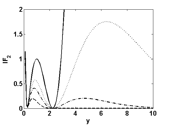
(a) Influence function of the test statistics

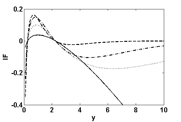
(b) Power Influence function

Figure 1: Influence functions of MDPDE based Wald-type test of (48) for different values of $\beta$ (solid line: $\beta=0$, dotted line: $\beta=0.3$, dashed-dotted line: $\beta=0.5$, dashed line: $\beta=1$).

Finally, let us examine the level and power stability of the proposed Wald-type test. Following the results derived in Section 4, the level influence function of any order will be zero at the null implying the robustness of its asymptotic level. Further, the power influence function of the Wald-type test at the contiguous alternatives $\theta_{n}$ is given by

$$\mathcal{PIF}({x},W_{\beta}^{0},F_{{\theta}_{0}})\cong K_{1}^{\ast}\left(\frac{d^{2}\eta_{\beta}^{2}}{\eta_{2\beta}}\right)\frac{d\eta_{\beta}}{\eta_{2\beta}}\left({1}+(1-x)\log x\right)e^{-\beta x},$$

where $K_{p}^{\ast}(s)$ is as defined in Theorem 8. Figure 1b shows the power influence function for some particular $\beta$. Once again, the power robustness of the proposed test for $\beta>0$ is clearly visible from the figure.

6.2 Test for Correlation in Bivariate Normal

Let us now consider another interesting hypothesis testing problem involving the correlation parameter of two normal populations with unknown means and variances; this problem often arises in several real life applications when we want to check for the association between any two sets of observation only assuming the normality of those two populations. Consider the observations $\boldsymbol{X}_{i}=(X_{i1},X_{i2})^{T}$, $i=1,\ldots,n$, from the bivariate normal model $\{\mathcal{N}(\boldsymbol{\mu},\boldsymbol{\Sigma})\}$ where $\boldsymbol{\mu}=(\mu_{1},\mu_{2})^{T}\in\mathbb{R}^{2}$ and

$$\boldsymbol{\Sigma}=\begin{pmatrix}\sigma_{1}^{2}&\rho\sigma_{1}\sigma_{2}\\ \rho\sigma_{1}\sigma_{2}&\sigma_{2}^{2}\end{pmatrix}$$

belongs to the set of $2\times 2$ positive definite matrices. Thus, our parameter of interest is $\boldsymbol{\theta}=(\mu_{1},\mu_{2},\sigma_{1},\sigma_{2},\rho)^{T}$ with the parameter space $\Theta=\mathbb{R}^{2}\times\mathbb{R}^{+}\times\mathbb{R}^{+}\times[-1,1]$. We want to test for the composite hypothesis

$$H_{0}:\rho=0\quad\text{against}\quad H_{1}:\rho\neq 0,$$ (49)

with values of $\mu_{1}$, $\mu_{2}$, $\sigma_{1}$ and $\sigma_{2}$ being unspecified. In terms of notations of Section 2, we have $r=1$ restrictions with $m(\boldsymbol{\theta})=\rho$ so that $\boldsymbol{M}(\boldsymbol{\theta})$ is a $5\times 1$ matrix with the last entry $1$ and rest $0$ and the null parameter space is $\Theta_{0}=\mathbb{R}^{2}\times\mathbb{R}^{+}\times\mathbb{R}^{+}\times\{0\}$. We shall now develop the Wald-type test statistic for this composite hypothesis along with its properties.

Using the form of the bivariate normal density, we can see that the MDPDE ${\boldsymbol{\widehat{\boldsymbol{\theta}}}}_{\beta}=(\widehat{\mu}_{1,\beta},\widehat{\mu}_{2,\beta},\widehat{\sigma}_{1,\beta},\widehat{\sigma}_{2,\beta},\widehat{\rho}_{\beta})^{T}$ of $\boldsymbol{\theta}$ with $\beta>0$ is the minimizer of

$$\frac{1}{(2\pi)^{\beta}\sigma_{1}^{\beta}\sigma_{2}^{\beta}(1-\rho^{2})^{\beta/2}}\left(\frac{1}{\sqrt{1+\beta}}-\frac{1+\beta}{n\beta}\sum_{i=1}^{n}e^{-\frac{\Upsilon(\boldsymbol{X}_{i},\boldsymbol{\theta})}{2}}\right),$$

with respect to $\boldsymbol{\theta}$, where $\Upsilon(\boldsymbol{x},\boldsymbol{\theta})=(\boldsymbol{x}-\boldsymbol{\theta})^{T}\boldsymbol{\Sigma}^{-1}(\boldsymbol{x}-\boldsymbol{\theta})$. Take any $\boldsymbol{\theta}_{0}=(\mu_{1,0},\mu_{2,0},\sigma_{1,0},\sigma_{2,0},0)^{T}\in\Theta_{0}$. Then the asymptotic variance of the MDPDE ${\boldsymbol{\widehat{\boldsymbol{\theta}}}}_{\beta}$ under $\boldsymbol{\theta}=\boldsymbol{\theta}_{0}$ is given by $\boldsymbol{\Sigma}_{\beta}(\boldsymbol{\theta}_{0})=\boldsymbol{J}_{\beta}^{-1}(\boldsymbol{\theta}_{0})\boldsymbol{K}_{\beta}(\boldsymbol{\theta}_{0})\boldsymbol{J}_{\beta}^{-1}(\boldsymbol{\theta}_{0})$. A straightforward but lengthy calculation shows that

$$\boldsymbol{J}_{\beta}(\boldsymbol{\theta}_{0})=\begin{pmatrix}\frac{C_{\beta}}{(1+\beta)^{3/2}\sigma_{1}^{2}}&0&0&0&0\\ 0&\frac{C_{\beta}}{(1+\beta)^{3/2}\sigma_{2}^{2}}&0&0&0\\ 0&0&\frac{(2+\beta^{2})C_{\beta}}{\sigma_{1}^{2}(1+\beta)^{5/2}}&\frac{\beta^{2}C_{\beta}}{\sigma_{1}\sigma_{2}(1+\beta)^{5/2}}&0\\ 0&0&\frac{\beta^{2}C_{\beta}}{\sigma_{1}\sigma_{2}(1+\beta)^{5/2}}&\frac{(2+\beta^{2})C_{\beta}}{\sigma_{2}^{2}(1+\beta)^{5/2}}&0\\ 0&0&0&0&\frac{C_{\beta}}{(1+\beta)^{5/2}}\end{pmatrix}$$

and

$$\boldsymbol{K}_{\beta}(\boldsymbol{\theta}_{0})=\begin{pmatrix}\frac{C_{2\beta}}{(1+2\beta)^{3/2}\sigma_{1}^{2}}&0&0&0&0\\ 0&\frac{C_{2\beta}}{(1+2\beta)^{3/2}\sigma_{2}^{2}}&0&0&0\\ 0&0&\frac{(2+3\beta^{2})C_{2\beta}}{\sigma_{1}^{2}(1+2\beta)^{5/2}}&\frac{3\beta^{2}C_{2\beta}}{\sigma_{1}\sigma_{2}(1+2\beta)^{5/2}}&0\\ 0&0&\frac{3\beta^{2}C_{2\beta}}{\sigma_{1}\sigma_{2}(1+2\beta)^{5/2}}&\frac{(2+3\beta^{2})C_{2\beta}}{\sigma_{2}^{2}(1+2\beta)^{5/2}}&0\\ 0&0&0&0&\frac{C_{2\beta}}{(1+2\beta)^{5/2}}\end{pmatrix}$$

where $C_{\beta}=(2\pi)^{-\beta}\sigma_{1}^{-\beta}\sigma_{2}^{-\beta}$ and $C_{\beta}^{\ast}=4C_{2\beta}-C_{\beta}^{2}$. Hence,

$$\boldsymbol{\Sigma}_{\beta}(\boldsymbol{\theta}_{0})=\begin{pmatrix}\zeta_{\beta}^{3/2}\sigma_{1}^{2}&0&0&0&0\\ 0&\zeta_{\beta}^{3/2}\sigma_{2}^{2}&0&0&0\\ 0&0&\zeta_{\beta}^{5/2}\kappa_{\beta}^{1}\sigma_{1}^{2}&\zeta_{\beta}^{5/2}\kappa_{\beta}^{2}\sigma_{1}\sigma_{2}&0\\ 0&0&\zeta_{\beta}^{5/2}\kappa_{\beta}^{2}\sigma_{1}\sigma_{2}&\zeta_{\beta}^{5/2}\kappa_{\beta}^{1}\sigma_{2}^{2}&0\\ 0&0&0&0&\zeta_{\beta}^{5/2}\end{pmatrix}$$

with

$$\zeta_{\beta}=1+\frac{\beta^{2}}{1+2\beta}\text{,}\quad\kappa_{\beta}^{1}=\frac{(\beta^{4}+5\beta^{2}+2)}{(1+\beta^{2})^{2}}\quad\text{and}\quad\kappa_{\beta}^{2}=\frac{\beta^{2}(1-\beta^{2})}{(1+\beta^{2})^{2}}.$$

Interestingly, note that whenever the null hypothesis $\rho=0$ is true the MDPDE of $\mu_{1}$, $\mu_{2}$ and $\rho$ are asymptotically independent of each other and also of the MDPDE of $\sigma_{1}$ and $\sigma_{2}$.

Now the robust Wald-type test statistic (18) for testing the null hypothesis (49) is given by

$$W_{n}({\boldsymbol{\widehat{\boldsymbol{\theta}}}}_{\beta})=n\frac{\widehat{\rho}_{\beta}^{2}}{\zeta_{\beta}^{5/2}},$$ (50)

which asymptotically follows a chi-square distribution with one degree of freedom under the null hypothesis. Note that, at $\beta=0$, $\widehat{\rho}_{\beta}$ coincides with the maximum likelihood estimator of $\rho$ and hence the proposed test $W_{n}$ coincides with the classical Wald test for the present problem. Further, under the contiguous alternatives $H_{1,n}^{\ast}:\rho_{n}=n^{-1/2}d$, the asymptotic distribution of $W_{n}({\boldsymbol{\widehat{\boldsymbol{\theta}}}}_{\beta})$ is a non-central chi-square distribution with one degree of freedom and non-centrality parameter $\zeta_{\beta}^{-5/2}d^{2}$. Note that, for any fixed level of significance, the asymptotic power of the Wald-type test under the contiguous alternative hypotheses decreases as the non-centrality parameter decreases and for any fixed $d$ it happens as $\beta$ increases. However, as we can see from Table 2, the loss in contiguous power of the Wald-type test is not very significant for smaller positive values of $\beta$.

Table 2: Asymptotic Power of the MDPDE based Wald-type test of (49) $5\%$ level of significance for different $\delta$ and $\beta$.

			$\beta$
	$d$		0	0.01	0.1	0.3	0.5	0.7	1
	0		0.050	0.050	0.050	0.050	0.050	0.050	0.050
	2		0.516	0.516	0.508	0.463	0.408	0.354	0.287
	3		0.851	0.851	0.844	0.800	0.735	0.662	0.553
	4		0.979	0.979	0.977	0.962	0.932	0.887	0.797
	5		0.999	0.999	0.999	0.997	0.991	0.978	0.937
	10		1.000	1.000	1.000	1.000	1.000	1.000	1.000

Now let us examine the robustness of this Wald-type test based on the results derived in the present paper. Note that the influence function of the minimum DPD functional $\boldsymbol{T}_{\beta}$ here under the null $\boldsymbol{\theta}=\boldsymbol{\theta}_{0}$ is given by

$$\mathcal{IF}(\boldsymbol{x},\boldsymbol{T}_{\beta},F_{\boldsymbol{\theta}_{0}})=\begin{pmatrix}(1+\beta)^{3/2}(x_{1}-\mu_{1})\\ (1+\beta)^{3/2}(x_{2}-\mu_{2})\\ \frac{(1+\beta)^{5/2}\sigma_{1}}{(1+\beta^{2})}\left(\frac{(2+\beta^{2})(x_{1}-\mu_{1})^{2}}{\sigma_{1}^{2}}-\frac{\beta^{2}(x_{2}-\mu_{2})^{2}}{\sigma_{2}^{2}}-2\right)\\ \frac{(1+\beta)^{5/2}\sigma_{2}}{(1+\beta^{2})}\left(\frac{(2+\beta^{2})(x_{2}-\mu_{2})^{2}}{\sigma_{2}^{2}}-\frac{\beta^{2}(x_{1}-\mu_{1})^{2}}{\sigma_{1}^{2}}-2\right)\\ (1+\beta)^{3/2}\frac{(x_{1}-\mu_{1})(x_{2}-\mu_{2})}{\sigma_{1}\sigma_{2}}\end{pmatrix}e^{-\frac{\beta}{2}\left(\frac{(x_{1}-\mu_{1})^{2}}{\sigma_{1}^{2}}+\frac{(x_{2}-\mu_{2})^{2}}{\sigma_{2}^{2}}\right)}-\begin{pmatrix}0\\ 0\\ \frac{\beta(1+\beta)^{2}}{(1+\beta^{2})}\sigma_{1}\\ \frac{\beta(1+\beta)^{2}}{(1+\beta^{2})}\sigma_{2}\\ 0\end{pmatrix}.$$

Using the result derived in Section 3, the first order influence function of the Wald-type test statistic $W_{\beta}$ is zero at the null and its second order influence function at the null is given by

$$\mathcal{IF}_{2}(\boldsymbol{x},W_{\beta},F_{\boldsymbol{\theta}_{0}})=\frac{2(1+2\beta)^{5/2}}{(1+\beta)^{2}\sigma_{1}^{2}\sigma_{2}^{2}}(x_{1}-\mu_{1})^{2}(x_{2}-\mu_{2})^{2}e^{-\beta\left(\frac{(x_{1}-\mu_{1})^{2}}{\sigma_{1}^{2}}+\frac{(x_{2}-\mu_{2})^{2}}{\sigma_{2}^{2}}\right)}.$$

Clearly, this influence function is unbounded at $\beta=0$, but whenever $\beta>0$ it is bounded implying the robustness of the corresponding test statistics. Figure 2 shows the plot of this influence function for some particular $\beta$. It is clear from the figures that the extend of the influence function over the contamination point $\boldsymbol{x}=(x_{1},~{}x_{2})^{T}$ decreases as $\beta$ increases. this fact can also bee seen by looking at the gross-error sensitivity of the test statistics given by

$$\gamma_{\beta}^{\ast}=\left\{\begin{array}[c]{lc}\frac{2n(1+2\beta)^{5/2}}{\sqrt{\beta}(1+\beta)^{2}}e^{-\sqrt{\beta}},&\text{if }\beta>0,\\ \infty,&\text{if }\beta=0.\end{array}\right.$$

Clearly $\gamma_{\beta}^{\ast}$ decreases as $\beta$ increases implying that the extent of robustness of the MDPDE based Wald-type test statistics increases.

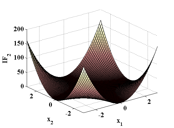
(a) $\beta=0$

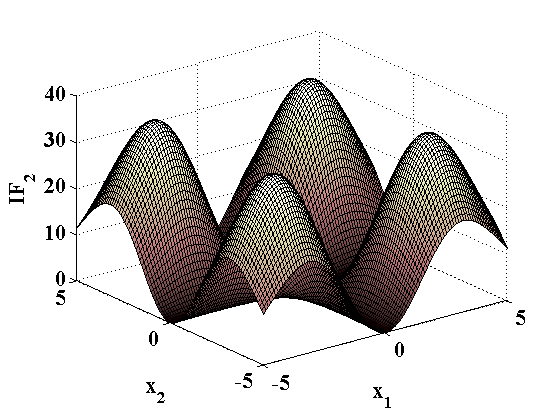
(b) $\beta=0.1$

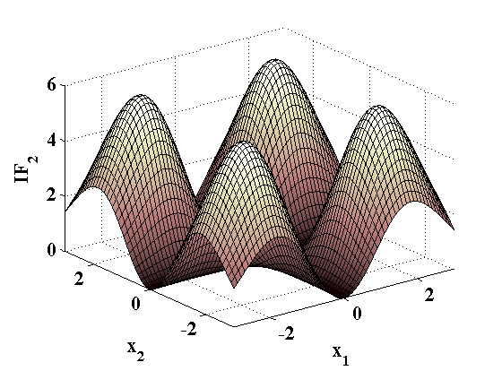
(c) $\beta=0.3$

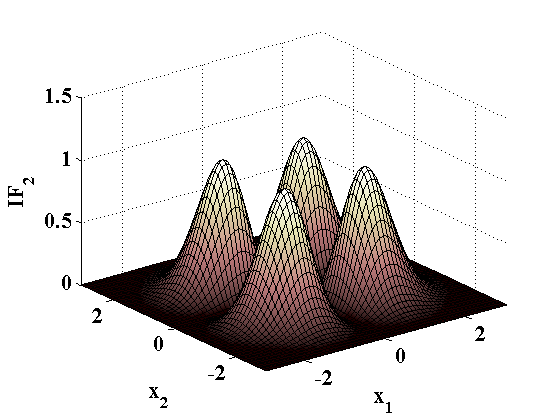
(d) $\beta=1$

Figure 2: Influence function of Wald-type test statistics for testing of (49) at the null for different values of $\beta$ (Here we have taken $\mu_{1}=\mu_{2}=0$ and $\sigma_{1}=\sigma_{2}=1$).

Next, we shall consider the level and power stability of the present test. As shown in Section 4.2, the level influence function of any order will be zero at the null hypothesis. Hence the level of the Wald-type test, constructed using asymptotic distribution, will be robust under infinitesimal contamination. On the other hand, if we consider the contamination proportion and the difference of alternatives $\rho_{n}$ from null converges to zero at the same rate of $n^{-1/2}$ ($\rho_{n}=n^{-1/2}d$), the power influence function of this test is given by

$$\mathcal{PIF}(\boldsymbol{x},W_{\beta},F_{\boldsymbol{\theta}_{0}})K_{1}^{\ast}\left(\zeta_{\beta}^{-5/2}d\right)\frac{(1+\beta)^{3/2}\zeta_{\beta}^{-5/2}d}{\sigma_{1}\sigma_{2}}(x_{1}-\mu_{1})(x_{2}-\mu_{2})e^{-\frac{\beta}{2}\left(\frac{(x_{1}-\mu_{1})^{2}}{\sigma_{1}^{2}}+\frac{(x_{2}-\mu_{2})^{2}}{\sigma_{2}^{2}}\right)},$$

where $K_{p}^{\ast}(s)$ is as defined in 3.

Again, it is clear that the above power influence function of the MDPDE based test statistic is bounded for all $\beta>0$ and unbounded at $\beta=0$ (see Figure 3). This justifies the power robustness of the proposed MDPDE based Wald-types tests with $\beta>0$ over the usual Wald test at $\beta=0$.

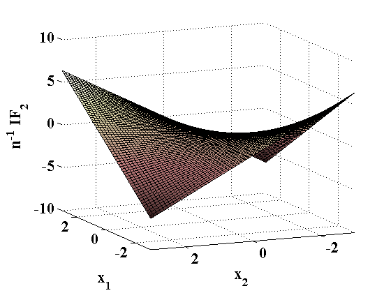
(a) $\beta=0$

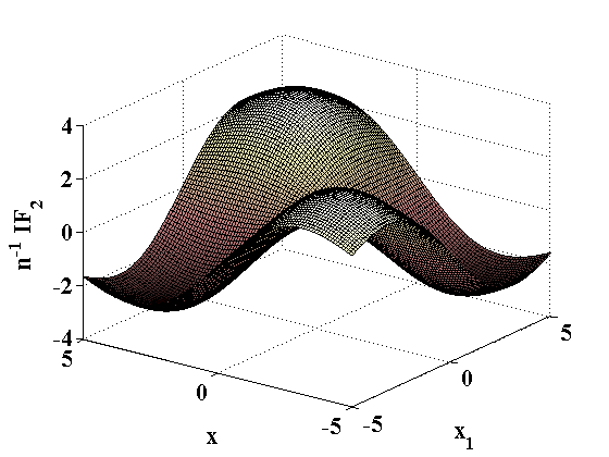
(b) $\beta=0.1$

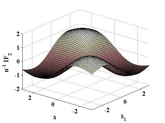
(c) $\beta=0.3$

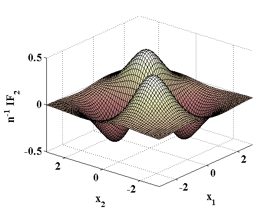
(d) $\beta=1$

Figure 3: Power influence function of Wald-type test of (48) at $5\%$ level of significance and $d=3$ for different values of $\beta$.

6.3 Test for the General Linear Hypothesis in Fixed-design Linear Regression Models

The robust minimum DPD estimators under the fixed-design Linear Regression Models are considered in Ghosh and Basu (2013), who have also derived their asymptotic and robustness properties in great detail (also see Ghosh and Basu (2015a)). Indeed, Ghosh and Basu (2013) considered a general class of models based on the non-homogeneous data and developed the theory of the MDPDE under that general set-up; the linear regression with pre-fixed (given) covariates comes as a special case of the general set-up. Under the same general set-up of independent but non-homogeneous data, Ghosh and Basu (2015b) have developed the divergence based tests of different kind of statistical hypothesis and discussed their properties and application in the fixed-design linear regression model. A nice study about robust M-type testing procedures for linear models can be seen in Markatou et al. (1991). Here, we briefly mention the corresponding Wald type test for only the class of general linear hypothesis and discuss their influence robustness following the theory developed in this paper.

Suppose we are given a fixed $n\times p$ design matrix, where the $i$-th value of the $p$ covariates are denoted as $\boldsymbol{x}_{i}=(x_{i1},\ldots,x_{ip})^{T}$ for $i=1,\ldots,n$. Consider the fixed-design linear regression model

$$y_{i}=\boldsymbol{x}_{i}^{T}{{\boldsymbol{\vartheta}}}+\epsilon_{i},~{}~{}i=1,\ldots,n,$$ (51)

where the error $\epsilon_{i}$’s are assumed to be i.i.d. normal with mean zero and variance $\sigma^{2}$ and ${{\boldsymbol{\vartheta}}}=(\vartheta_{1},\ldots,\vartheta_{p})^{T}$ denote the vector of regression coefficients. Then, for each $i$, $y_{i}\sim\mathcal{N}(\boldsymbol{x}_{i}^{T}{{\boldsymbol{\vartheta}}},\sigma^{2})$ which are clearly independent but not identically distributed.

Following Ghosh and Basu (2013), we can derive the $\sqrt{n}$-consistent MDPDE $\widehat{{\boldsymbol{\theta}}}_{\beta}=(\widehat{{\boldsymbol{\vartheta}}}_{\beta}^{T},~{}\widehat{\sigma}_{\beta}^{2})^{T}$ of the parameters ${{\boldsymbol{\theta}}}=({{\boldsymbol{\vartheta}}}^{T},~{}\sigma^{2})^{T}$ with tuning parameter $\beta$, which are asymptotically independent normally distributed under conditions (R1)–(R2) of Ghosh and Basu (2013). In particular, if ${{\boldsymbol{\vartheta}}}_{0}$ and $\sigma_{0}^{2}$ are the true values of the parameters then we have

$$\sqrt{n}(\boldsymbol{X}^{T}\boldsymbol{X})^{1/2}(\widehat{{\boldsymbol{\vartheta}}}_{\beta}-{{\boldsymbol{\vartheta}}}_{0})\underset{n\rightarrow\infty}{\overset{\mathcal{L}}{\longrightarrow}}\mathcal{N}_{p}\left(0,\zeta_{\beta}^{3/2}\sigma_{0}^{2}\right),$$ (52)

$$\sqrt{n}(\widehat{\sigma}_{\beta}^{2}-\sigma_{0}^{2})\underset{n\rightarrow\infty}{\overset{\mathcal{L}}{\longrightarrow}}\mathcal{N}(0,4\zeta_{\beta}^{5/2}\kappa_{\beta}^{1}\sigma_{0}^{4}),$$ (53)

where $\zeta_{\beta}$ and $\kappa_{\beta}^{1}$ are as defined Section 6.2 and $\boldsymbol{X}=[\boldsymbol{x}_{1}~{}\boldsymbol{x}_{2}~{}\cdots~{}\boldsymbol{x}_{n}]^{T}$.

Now, let us consider the class of general linear hypothesis on $\boldsymbol{\vartheta}$ with unspecified $\sigma$ as given by

$$H_{0}:\boldsymbol{L}^{T}\boldsymbol{\vartheta}=\boldsymbol{l_{0}}\qquad\text{against}\qquad H_{1}:\boldsymbol{L}^{T}\boldsymbol{\vartheta}\neq\boldsymbol{l_{0}},$$ (54)

where the $p\times r$ matrix $\boldsymbol{L}$ is known with rank $r(\leq p)$ and $l_{0}$ is a known $r$-vector. Due to full row rank of the matrix $\boldsymbol{L}$, there exists a true parameter value $\boldsymbol{\vartheta}_{0}$ satisfying the null hypothesis $\boldsymbol{L}^{T}\boldsymbol{\vartheta}_{0}=\boldsymbol{l_{0}}$. In particular, this general class of linear hypothesis consider the popular problem of testing the significance of the model $H_{0}:\boldsymbol{\vartheta}=\boldsymbol{\vartheta_{0}}$ where $r=p$, $\boldsymbol{l_{0}}=\boldsymbol{\vartheta_{0}}$ (usually a zero vector) and $\boldsymbol{L}=\boldsymbol{I}_{p}$, the identity matrix of order $p$. Also the test of significance of any one regression component $H_{0}:\vartheta_{j}=\vartheta_{0j}$ belongs to the class of hypothesis (54) with $r=1$, $\boldsymbol{l_{0}}=\vartheta_{0j}$ and $\boldsymbol{L}$ is $p$-vector of zeros except the $j$-th component which is $1$.

In the notation of Section 2.2, here we have $\boldsymbol{m}^{T}\left({\boldsymbol{\theta}}\right)=\boldsymbol{m}^{T}\left({\boldsymbol{\vartheta}},{\sigma^{2}}\right)=\boldsymbol{L}^{T}\boldsymbol{\vartheta}-\boldsymbol{l_{0}}$ and $\boldsymbol{M}\left({\boldsymbol{\theta}}\right)=\boldsymbol{M}\left({\boldsymbol{\vartheta}},{\sigma^{2}}\right)=\begin{pmatrix}\boldsymbol{L}^{T}&\boldsymbol{0}_{r}\\ \boldsymbol{0}_{p}^{T}&0\end{pmatrix}$. Hence, the Wald-type test for this general linear hypothesis in (54) is given by

$$W_{n}(\widehat{{\boldsymbol{\vartheta}}}_{\beta},\widehat{\sigma}_{\beta}^{2})=\frac{n}{\zeta_{\beta}^{3/2}\widehat{\sigma}_{\beta}^{2}}(\boldsymbol{L}^{T}\widehat{{\boldsymbol{\vartheta}}}_{\beta}-\boldsymbol{l_{0}})^{T}\left(\boldsymbol{L}^{T}(\boldsymbol{X}^{T}\boldsymbol{X})^{-1}\boldsymbol{L}\right)^{-1}(\boldsymbol{L}^{T}\widehat{{\boldsymbol{\vartheta}}}_{\beta}-\boldsymbol{l_{0}}),$$ (55)

which asymptotically follows $\chi_{r}^{2}$ distribution under the null hypothesis. Also, under the contiguous alternative $H_{1n}^{\ast}$ in (21), given by $\boldsymbol{L}^{T}{\boldsymbol{\vartheta}}=\boldsymbol{l_{0}}+n^{-1/2}\boldsymbol{\delta}$, the asymptotic distribution of the test statistics $W_{n}(\widehat{{\boldsymbol{\theta}}}_{\beta},\widehat{\sigma}_{\beta}^{2})$ is non-central chi-square with the non-centrality parameter $\omega_{\beta}$ defined as

$$\omega_{\beta}=\zeta_{\beta}^{-3/2}\sigma_{0}^{-2}\boldsymbol{\delta}^{T}\left(\boldsymbol{L}^{T}(\boldsymbol{X}^{T}\boldsymbol{X})^{-1}\boldsymbol{L}\right)^{-1}\boldsymbol{\delta}.$$

Now, let us derive the influence functions of the above Wald-type test statistics. However, as noted in Ghosh and Basu (2013, 2015b), in this case of non-homogeneous observations, the corresponding statistical functional and the influence functions will depend on the sample size through the given values of covariates $\boldsymbol{x}_{i}$’s. In particular, we need to assume that the true distributions of each $y_{i}$ are (possibly) different, say $H_{i}$ ($i=1,\ldots,n$), depending on the given values of $x_{i}$. Then, the statistical functional corresponding to the Wald-type test (55) is given by

$$W_{\beta}\left(H_{1},\ldots,H_{n}\right)=\zeta_{\beta}^{-3/2}\left(\boldsymbol{L}^{T}\boldsymbol{T}_{\beta}^{\vartheta}(H_{1},\ldots,H_{n})-\boldsymbol{l_{0}}\right)^{T}\frac{\left(\boldsymbol{L}^{T}(\boldsymbol{X}^{T}\boldsymbol{X})^{-1}\boldsymbol{L}\right)^{-1}}{T_{\beta}^{\sigma}(H_{1},\ldots,H_{n})}\left(\boldsymbol{L}^{T}\boldsymbol{T}_{\beta}^{\vartheta}(H_{1},\ldots,H_{n})-\boldsymbol{l_{0}}\right),$$

where $\boldsymbol{T}_{\beta}^{\vartheta}$ and $T_{\beta}^{\sigma}$ are the statistical functionals corresponding to the MDPDEs $\widehat{{\boldsymbol{\vartheta}}}_{\beta}$ and $\widehat{\sigma}_{\beta}^{2}$, as defined in Ghosh and Basu (2013). Since there are $n$ many different distributions, we can assume the contamination in any one of these distributions or in all the distributions. Corresponding influence functions of the MDPDEs are derived in Ghosh and Basu (2013). Using them and following the arguments used to proof Theorem 1, we get the influence functions of the proposed Wald type test. In particular, at the null hypothesis, the first order influence function is zero for any kind of contamination and the second order influence function at the null is given by

$$\mathcal{IF}_{2}(t_{i};W_{\beta},F_{\boldsymbol{\theta}_{0}})=2(1+\beta)^{3}\zeta_{\beta}^{-3/2}\sigma_{0}^{-2}(t_{i}-\boldsymbol{x}_{i}^{T}\boldsymbol{\vartheta}_{0})^{2}\boldsymbol{x}_{i}^{T}\boldsymbol{D}\boldsymbol{x}_{i}e^{-\frac{\beta(t_{i}-\boldsymbol{x}_{i}^{T}\boldsymbol{\vartheta}_{0})^{2}}{\sigma_{0}^{2}}},~{}~{}~{}~{}~{}\boldsymbol{\theta}_{0}=(\boldsymbol{\vartheta}_{0}^{T},\sigma_{0}^{2})^{T},$$

if the contamination is only in $i$-th direction at the point $t_{i}$, and

$$\mathcal{IF}_{2}(t_{1},\ldots,t_{n};W_{\beta},F_{\boldsymbol{\theta}_{0}})=2(1+\beta)^{3}\zeta_{\beta}^{-3/2}\sigma_{0}^{-2}\sum_{i=1}^{n}(t_{i}-\boldsymbol{x}_{i}^{T}\boldsymbol{\vartheta}_{0})^{2}\boldsymbol{x}_{i}^{T}\boldsymbol{D}\boldsymbol{x}_{i}e^{-\frac{\beta(t_{i}-\boldsymbol{x}_{i}^{T}\boldsymbol{\vartheta}_{0})^{2}}{\sigma_{0}^{2}}},$$

if there is contamination in all the directions at the points $t_{i}$’s. Here

$$\boldsymbol{D}=(\boldsymbol{X}^{T}\boldsymbol{X})^{-1}\boldsymbol{L}\left(\boldsymbol{L}^{T}(\boldsymbol{X}^{T}\boldsymbol{X})^{-1}\boldsymbol{L}\right)^{-1}\boldsymbol{L}^{T}(\boldsymbol{X}^{T}\boldsymbol{X})^{-1}.$$

Next we consider the level and power influence functions of the proposed Wald-type test. As in Section 4.2, it follows that the level influence function is always zero implying the level robustness of the proposal. For power influence function, we again consider the alternatives $H_{1n}^{\ast}:\boldsymbol{L}^{T}{\boldsymbol{\vartheta}}=\boldsymbol{l_{0}}+n^{-1/2}\boldsymbol{\delta}$ and proceed as in Section 4.2 to obtain the PIF for different types of contamination. In particular, for contamination only in the $i$-th direction at the point $t_{i}$ we get

$$\mathcal{PIF}(t_{i};W_{\beta},F_{\boldsymbol{\theta}_{0}})=\frac{K_{r}^{\ast}(\omega_{\beta})(1+\beta)^{3/2}}{\zeta_{\beta}^{3/2}\sigma_{0}^{2}}\left[\boldsymbol{\delta}^{T}\boldsymbol{D}_{P}\boldsymbol{x_{i}}\right](t_{i}-\boldsymbol{x}_{i}^{T}\boldsymbol{\vartheta_{0}})e^{-\frac{\beta(t_{i}-\boldsymbol{x}_{i}^{T}\boldsymbol{\vartheta_{0}})^{2}}{2\sigma_{0}^{2}}},$$

where

$$\boldsymbol{D}_{P}=\left(\boldsymbol{L}^{T}(\boldsymbol{X}^{T}\boldsymbol{X})^{-1}\boldsymbol{L}\right)^{-1}\boldsymbol{L}^{T}(\boldsymbol{X}^{T}\boldsymbol{X})^{-1}$$

Similarly, if the contamination is assumed to be in all the directions at the points $t_{i}$s ($i=1,\ldots,n$), the corresponding power influence function is given by

$$\mathcal{PIF}(t_{1},\ldots,t_{n};W_{\beta},F_{\boldsymbol{\theta}_{0}})=\frac{K_{r}^{\ast}(\omega_{\beta})(1+\beta)^{3/2}}{\zeta_{\beta}^{3/2}\sigma_{0}^{2}}\boldsymbol{\delta}^{T}\boldsymbol{D}_{P}\sum_{i=1}^{n}\boldsymbol{x_{i}}(t_{i}-\boldsymbol{x}_{i}^{T}\boldsymbol{\vartheta_{0}})e^{-\frac{\beta(t_{i}-\boldsymbol{x}_{i}^{T}\boldsymbol{\vartheta_{0}})^{2}}{2\sigma_{0}^{2}}}.$$

Clearly, the power influence function is bounded for all $\beta>0$ implying robustness and unbounded at $\beta=0$ implying the non-robust nature of the classical Wald test.

Remark 14

For the testing of significance of regression model ($H_{0}:\boldsymbol{\vartheta}=\boldsymbol{0}_{p}$) we have $r=p$, $\boldsymbol{l}_{0}=\boldsymbol{0}_{p}$ and $L=I_{p}$, the identity matrix of order $p$. In this case the Wald-Type test statistic (55) simplifies to

$$W_{n}(\widehat{{\boldsymbol{\vartheta}}}_{\beta},\widehat{\sigma}_{\beta}^{2})=\frac{n}{\zeta_{\beta}^{3/2}\widehat{\sigma}_{\beta}^{2}}\widehat{{\boldsymbol{\vartheta}}}_{\beta}^{T}(\boldsymbol{X}^{T}\boldsymbol{X})\widehat{{\boldsymbol{\vartheta}}}_{\beta},$$

which is asymptotically $\chi_{p}^{2}$ under the null hypothesis. Under the contiguous alternatives $H_{1n}^{\ast}$, its asymptotic distribution becomes the non-central chi-square with $p$ degrees of freedom and non-centrality parameter $\omega_{\beta}=\zeta_{\beta}^{-3/2}\sigma_{0}^{-2}\boldsymbol{\delta}^{T}(\boldsymbol{X}^{T}\boldsymbol{X})\boldsymbol{\delta}$. Noting that the asymptotic distribution under the contiguous alternatives depends on the tuning parameter $\beta$ only through the quantity $zeta_{\beta}$ and examining its form, one can easily check that the asymptotic contiguous power of the proposed Wald-type tests decreases only slightly with increasing values of $\beta$ so that the power loss under pure data is not significant at small positive values of $\beta$.

On the other hand, under contamination we gain high robustness with these positive values of $\beta$. For illustrations, we have presented (Figure 4) the form of the second order influence function of the tests and the power influence function for various values of $\beta$ under contamination in one direction (say $i$-th). In this special case, they have the simplified form (with $\boldsymbol{\vartheta}_{0}=\boldsymbol{0}_{p}$)

$$\mathcal{IF}_{2}(t_{i};W_{\beta},F_{\boldsymbol{\theta}_{0}})=2(1+\beta)^{3}\zeta_{\beta}^{-3/2}\sigma_{0}^{-2}\left[\boldsymbol{x}_{i}^{T}(\boldsymbol{X}^{T}\boldsymbol{X})^{-1}\boldsymbol{x}_{i}\right]t_{i}^{2}e^{-\frac{\beta t_{i}^{2}}{\sigma_{0}^{2}}},$$

and

$$\mathcal{PIF}(t_{i};W_{\beta},F_{\boldsymbol{\theta}_{0}})=\frac{K_{r}^{\ast}(\omega_{\beta})(1+\beta)^{3/2}}{\zeta_{\beta}^{3/2}\sigma_{0}^{2}}\left[\boldsymbol{\delta}^{T}\boldsymbol{x_{i}}\right]t_{i}e^{-\frac{\beta t_{i}^{2}}{2\sigma_{0}^{2}}}.$$

It is clear from the figure that the influence functions are bounded for all $\beta>0$ and their maximum values decreases as $\beta$ increases implying the increasing robustness.

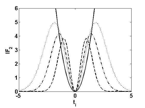
(a) IF of the test statistics with $\boldsymbol{x}_{i}^{T}(\boldsymbol{X}^{T}\boldsymbol{X})^{-1}\boldsymbol{x}_{i}=1$

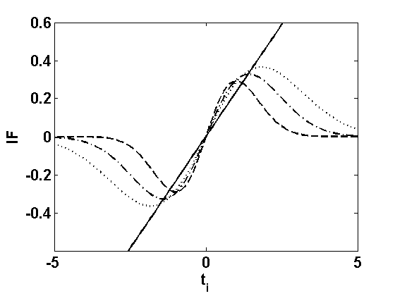
(b) PIF with $\boldsymbol{\delta}^{T}\boldsymbol{x_{i}}=1$ and $\boldsymbol{\delta}^{T}(\boldsymbol{X}^{T}\boldsymbol{X})\boldsymbol{\delta}=3$

Figure 4: Influence functions of MDPDE based Wald-type test of (54) with $\sigma_{0}=1$ for different values of $\beta$ (solid line: $\beta=0$, dotted line: $\beta=0.3$, dashed-dotted line: $\beta=0.5$, dashed line: $\beta=1$).

7 On the Choice of Tuning Parameter $\beta$

After deriving several important properties of the Wald-type test, a natural question that arises from the point of view of a practitioner is what value of the tuning parameter should be used for a particular dataset. For the MDPDE the role of the tuning parameter $\beta$ has been well studied in the literature, which indicates that robustness increases with $\beta$, but efficiency decreases at the same time. So $\beta$ is selected that gives a trade-off between robustness and efficiency of the estimator. However, a small positive value of $\beta$ is generally recommended that provides enough robustness with a slight loss in efficiency (see Basu et al., 1998 and Basu et al., 2011). Broniatowski et al. (2012) have reported that values of $\beta\in[0.1,0.25]$ are often reasonable choices. We largely agree with this view, although tentative outliers and heavier contamination may require a larger value of $\beta$ in some cases. Apart from a fixed choice of the tuning parameter, one may dynamically select an optimum value of $\beta$ based on the real data. Hong and Kim (2001) and Warwick and Jones (2005) have provided some data driven choices of $\beta$ for the MDPDE. In case of hypothesis testing the optimality criteria are different from the estimation case. Here the asymptotic power against the contiguous alternative may be regarded as a measure of efficiency of the test, which decreases with $\beta$. On the other hand, the robustness of the test against contamination increases as $\beta$ increases. Therefore, our suggestion in this regard is to choose an optimum value of $\beta$ that gives a suitable trade-off between the asymptotic power against the contiguous alternative and a robustness measure, see Ghosh and Basu (2015c) for details. As the robustness of the Wald-type test statistic depends primarily on the robustness of the estimators, another simple criterion to choose an optimum value of $\beta$ is to focus on the same optimum value for the estimator.

To avoid selecting a unique and specific tuning parameter, one may construct a test combining a set of Wald-type tests corresponding to different $\beta$. Lavancier and Rochet (2014) have derived a general procedure to combine a set of estimators. This idea of constructing combined tests might be incorporated.

8 Concluding Remarks

Basu et al. (2015) have proposed the Wald-type test statistics based on the minimum density power divergence estimators. They have observed strong robustness properties of the tests by using extensive simulation results. In this paper we have given proper theoretical foundations behind the robustness properties of the Wald-type test statistics. The influence function analysis is carried out to observe the effect of an infinitesimal contamination on the test statistics. To justify the stability of the level and power under a contaminated distribution we have studied the level and power influence functions. It is shown that the level influence function of a Wald-type test statistic is zero, so the level of the test remains unchanged in infinitesimal contamination. For the contiguous alternative the power influence function is bounded whenever the influence function of the MDPDE is bounded. Other than location-scale parameters for the normal model we have shown some examples where the power influence functions are bounded, and it gives the theoretical justification behind the stability of the power function. On the other hand, the power influence functions of the classical Wald tests are unbounded, and as a result they exhibit poor power in contaminated data. We have also proposed the chi-square inflation factor to measure the robustness property with respect to the model assumption, and studied its infinitesimal change for the Wald-type test statistics. On the whole, we hope that this research establishes that the tests proposed by Basu et al. (2015) not only perform well in practise, but also have theoretically sound robustness credentials.

Acknowledgements: The authors would like to acknowledge the comments of the three referess, since they helped improving the paper.

Appendix A Appendix

There is some overlap between the Lehmann and Basu et al. conditions. In the following we present the consolidated set of conditions which are the useful ones in our context.

A.1 Lehmann and Basu et al. conditions

• The model distributions $F_{\boldsymbol{\theta}}$ of $\boldsymbol{X}$ have common support, so that the set $\mathcal{X}=\{\boldsymbol{x}|f_{\boldsymbol{\theta}}(\boldsymbol{x})>0\}$ is independent of $\boldsymbol{\theta}$. The true distribution $H$ is also supported on $\mathcal{X}$, on which the corresponding density $h$ is greater than zero.

• There is an open subset of $\omega$ of the parameter space $\Theta$, containing the best fitting parameter $\boldsymbol{\theta}_{0}$ such that for almost all $\boldsymbol{x}\in\mathcal{X}$, and all $\boldsymbol{\theta}\in\omega$, the density $f_{\boldsymbol{\theta}}(\boldsymbol{x})$ is three times differentiable with respect to $\boldsymbol{\theta}$ and the third partial derivatives are continuous with respect to $\boldsymbol{\theta}$.

• The integrals $\int f_{\boldsymbol{\theta}}^{1+\beta}(\boldsymbol{x})d\boldsymbol{x}$ and $\int f_{\boldsymbol{\theta}}^{\beta}(\boldsymbol{x})h(\boldsymbol{x})d\boldsymbol{x}$ can be differentiated three times with respect to $\boldsymbol{\theta}$, and the derivatives can be taken under the integral sign.

• The $p\times p$ matrix $\boldsymbol{J}_{\beta}(\boldsymbol{\theta})$, defined in (6), is positive definite.

• There exists a function $M_{jkl}(\boldsymbol{x})$ such that $|\nabla_{jkl}V_{\boldsymbol{\theta}}(\boldsymbol{x})|\leq M_{jkl}(\boldsymbol{x})$ for all $\boldsymbol{\theta}\in\omega$, where $V_{\theta}(\boldsymbol{x})=\int f_{\boldsymbol{\theta}}^{1+\beta}(\boldsymbol{y})d\boldsymbol{y}-\left(1+\tfrac{1}{\beta}\right)f_{\boldsymbol{\theta}}^{\beta}(\boldsymbol{x})$ and $E_{h}[M_{jkl}(\boldsymbol{X})]=m_{jkl}<\infty$ for all $j$, $k$ and $l$.

A.2 Proof of Theorem 1

The second order influence function of $W_{\beta}^{0}(\cdot)$ is given by

$$\mathcal{IF}_{2}(\boldsymbol{x},W_{\beta}^{0},G)=\left.\frac{\partial^{2}W_{\beta}^{0}(G_{\varepsilon})}{\partial\varepsilon^{2}}\right|_{\varepsilon=0},$$

and

$$\left.\frac{\partial^{2}W_{\beta}^{0}(G_{\varepsilon})}{\partial\varepsilon^{2}}\right|_{\varepsilon=0} =2\mathcal{IF}^{T}(\boldsymbol{x},\boldsymbol{T}_{\beta},G)\boldsymbol{\Sigma}_{\beta}^{-1}(\boldsymbol{\theta}_{0})\mathcal{IF}(\boldsymbol{x},\boldsymbol{T}_{\beta},G)$$

$$+2(\boldsymbol{T}_{\beta}(G)-\boldsymbol{\theta}_{0})^{T}\boldsymbol{\Sigma}_{\beta}^{-1}(\boldsymbol{\theta}_{0})\mathcal{IF}_{2}(\boldsymbol{x},\boldsymbol{T}_{\beta},G).$$

As $\boldsymbol{T}_{\beta}(F_{\boldsymbol{\theta}_{0}})=\boldsymbol{\theta}_{0}$, we obtain

$$\mathcal{IF}_{2}(\boldsymbol{x},W_{\beta}^{0},F_{\boldsymbol{\theta}_{0}})=2\mathcal{IF}^{T}(\boldsymbol{x},\boldsymbol{T}_{\beta},F_{\boldsymbol{\theta}_{0}})\boldsymbol{\Sigma}_{\beta}^{-1}(\boldsymbol{\theta}_{0})\mathcal{IF}(\boldsymbol{x},\boldsymbol{T}_{\beta},F_{\boldsymbol{\theta}_{0}}).$$

The second order influence function of (29) is given by

$$\mathcal{IF}_{2}(\boldsymbol{x},W_{\beta},G)=\left.\frac{\partial^{2}W_{\beta}(G_{\varepsilon})}{\partial\varepsilon^{2}}\right|_{\varepsilon=0},$$

and

$$\left.\frac{\partial^{2}W_{\beta}(G_{\varepsilon})}{\partial\varepsilon^{2}}\right|_{\varepsilon=0} =2\mathcal{IF}^{T}(\boldsymbol{x},\boldsymbol{T}_{\beta},G)\boldsymbol{M}(\boldsymbol{T}_{\beta}(G))\left(\boldsymbol{M}^{T}(\boldsymbol{T}_{\beta}(G))\boldsymbol{\Sigma}_{\beta}(\boldsymbol{T}_{\beta}(G))\boldsymbol{M}(\boldsymbol{T}_{\beta}(G))\right)^{-1}\boldsymbol{M}^{T}(\boldsymbol{T}_{\beta}(G))\mathcal{IF}(\boldsymbol{x},\boldsymbol{T}_{\beta},G)$$

$$+2\boldsymbol{m}^{T}(\boldsymbol{T}_{\beta}(G))\left.\frac{\partial}{\partial\varepsilon}\left(\left(\boldsymbol{M}^{T}(\boldsymbol{T}_{\beta}(G_{\varepsilon}))\boldsymbol{\Sigma}_{\beta}(\boldsymbol{T}_{\beta}(G_{\varepsilon}))\boldsymbol{M}(\boldsymbol{T}_{\beta}(G_{\varepsilon}))\right)^{-1}\boldsymbol{M}^{T}(\boldsymbol{T}_{\beta}(G_{\varepsilon}))\mathcal{IF}(\boldsymbol{x},\boldsymbol{T}_{\beta},G_{\varepsilon})\right)\right|_{\varepsilon=0}$$

$$+2\boldsymbol{m}^{T}(\boldsymbol{T}_{\beta}(G))\left.\frac{\partial}{\partial\varepsilon}\left(\left(\boldsymbol{M}^{T}(\boldsymbol{T}_{\beta}(G_{\varepsilon}))\boldsymbol{\Sigma}_{\beta}(\boldsymbol{T}_{\beta}(G_{\varepsilon}))\boldsymbol{M}(\boldsymbol{T}_{\beta}(G_{\varepsilon}))\right)^{-1}\right)\right|_{\varepsilon=0}\boldsymbol{M}^{T}(\boldsymbol{T}_{\beta}(G))\mathcal{IF}(\boldsymbol{x},\boldsymbol{T}_{\beta},G)$$

$$+\boldsymbol{m}^{T}(\boldsymbol{T}_{\beta}(G))\left.\frac{\partial^{2}}{\partial\varepsilon^{2}}\left(\left(\boldsymbol{M}^{T}(\boldsymbol{T}_{\beta}(G_{\varepsilon}))\boldsymbol{\Sigma}_{\beta}(\boldsymbol{T}_{\beta}(G_{\varepsilon}))\boldsymbol{M}(\boldsymbol{T}_{\beta}(G_{\varepsilon}))\right)^{-1}\right)\right|_{\varepsilon=0}\boldsymbol{m}(\boldsymbol{T}_{\beta}(G))$$

$$=2\mathcal{IF}^{T}(\boldsymbol{x},\boldsymbol{T}_{\beta},G)\boldsymbol{M}(\boldsymbol{T}_{\beta}(G))\left[\boldsymbol{M}^{T}(\boldsymbol{T}_{\beta}(G))\boldsymbol{\Sigma}_{\beta}(\boldsymbol{T}_{\beta}(G))\boldsymbol{M}(\boldsymbol{T}_{\beta}(G))\right]^{-1}\boldsymbol{M}^{T}(\boldsymbol{T}_{\beta}(G))\mathcal{IF}(\boldsymbol{x},\boldsymbol{T}_{\beta},G)$$

$$=2\left(\boldsymbol{u}_{\boldsymbol{\theta}}\left(\boldsymbol{x}\right)f_{\boldsymbol{\theta}_{0}}^{\beta}(\boldsymbol{x})-\boldsymbol{\xi}\left(\boldsymbol{\theta}_{0}\right)\right)^{T}\boldsymbol{J}_{\beta}^{-1}(\boldsymbol{\theta}_{0})\boldsymbol{M}(\boldsymbol{\theta}_{0})\left(\boldsymbol{M}^{T}(\boldsymbol{\theta}_{0})\boldsymbol{\Sigma}_{\beta}(\boldsymbol{\theta}_{0})\boldsymbol{M}(\boldsymbol{\theta}_{0})\right)^{-1}$$

$$\times\boldsymbol{M}^{T}(\boldsymbol{\theta}_{0})\boldsymbol{J}_{\beta}^{-1}(\boldsymbol{\theta}_{0})\left(\boldsymbol{u}_{\boldsymbol{\theta}}\left(\boldsymbol{x}\right)f_{\boldsymbol{\theta}_{0}}^{\beta}(\boldsymbol{x})-\boldsymbol{\xi}\left(\boldsymbol{\theta}_{0}\right)\right),$$

As $\boldsymbol{T}_{\beta}(F_{\boldsymbol{\theta}_{0}})=\boldsymbol{\theta}$₀, we obtain

$$\mathcal{IF}_{2}(\boldsymbol{x},W_{\beta},F_{\boldsymbol{\theta}_{0}}) =2\mathcal{IF}^{T}(\boldsymbol{x},\boldsymbol{T}_{\beta},F_{\boldsymbol{\theta}_{0}})\boldsymbol{M}(\boldsymbol{\theta}_{0})\left(\boldsymbol{M}^{T}(\boldsymbol{\theta}_{0})\boldsymbol{\Sigma}_{\beta}(\boldsymbol{\theta}_{0})\boldsymbol{M}(\boldsymbol{\theta}_{0})\right)^{-1}$$

$$\times\boldsymbol{M}^{T}(\boldsymbol{\theta}_{0})\mathcal{IF}(\boldsymbol{x},\boldsymbol{T}_{\beta},F_{\boldsymbol{\theta}_{0}}).$$

A.3 Proof of Theorem 3

Let us denote the quadratic form of a symmetric matrix $\boldsymbol{A}_{p\times p}$ as $q_{\boldsymbol{A}}(\boldsymbol{z})=\boldsymbol{z}^{T}\boldsymbol{A}\boldsymbol{z}$. We shall frequently use the following result that

$$q_{\boldsymbol{A}}(\boldsymbol{z}+\boldsymbol{h})=q_{\boldsymbol{A}}(\boldsymbol{z})+2\boldsymbol{h}^{T}\boldsymbol{A}\boldsymbol{z}+q_{\boldsymbol{A}}(\boldsymbol{h}),$$ (56)

where $\boldsymbol{z}$ and $\boldsymbol{h}$ are two vectors in $\mathbb{R}^{p}$. Using $\boldsymbol{\theta}$${}_{n}^{\ast}=\boldsymbol{T}_{\beta}(F_{n,\varepsilon,\boldsymbol{x}}^{P})$ and equation (56), with $\boldsymbol{z=}\widehat{\boldsymbol{\theta}}_{\beta}-$$\boldsymbol{\theta}$${}_{n}^{\ast}$ and $\boldsymbol{h=}$$\boldsymbol{\theta}$${}_{n}^{\ast}-$$\boldsymbol{\theta}$₀, we get

$$W_{n}^{0}(\widehat{\boldsymbol{\theta}}_{\beta}) =q_{n\boldsymbol{\Sigma}_{\beta}^{-1}(\boldsymbol{\theta}_{0})}(\widehat{\boldsymbol{\theta}}_{\beta}-\boldsymbol{\theta}_{0})=q_{n\boldsymbol{\Sigma}_{\beta}^{-1}(\boldsymbol{\theta}_{0})}\left((\widehat{\boldsymbol{\theta}}_{\beta}-\boldsymbol{\theta}_{n}^{\ast})+(\boldsymbol{\theta}_{n}^{\ast}-\boldsymbol{\theta}_{0})\right)$$

$$=q_{n\boldsymbol{\Sigma}_{\beta}^{-1}(\boldsymbol{\theta}_{0})}(\widehat{\boldsymbol{\theta}}_{\beta}-\boldsymbol{\theta}_{n}^{\ast})+2n(\widehat{\boldsymbol{\theta}}_{\beta}-\boldsymbol{\theta}_{n}^{\ast})^{T}\boldsymbol{\Sigma}_{\beta}^{-1}(\boldsymbol{\theta}_{0})(\boldsymbol{\theta}_{n}^{\ast}-\boldsymbol{\theta}_{0})+q_{n\boldsymbol{\Sigma}_{\beta}^{-1}(\boldsymbol{\theta}_{0})}(\boldsymbol{\theta}_{n}^{\ast}-\boldsymbol{\theta}_{0}),$$

i.e.,

$$W_{n}^{0}(\widehat{\boldsymbol{\theta}}_{\beta})=W_{n}^{0}(\boldsymbol{\theta}_{n}^{\ast})+q_{n\boldsymbol{\Sigma}_{\beta}^{-1}(\boldsymbol{\theta}_{0})}(\widehat{\boldsymbol{\theta}}_{\beta}-\boldsymbol{\theta}_{n}^{\ast})+2n(\widehat{\boldsymbol{\theta}}_{\beta}-\boldsymbol{\theta}_{n}^{\ast})^{T}\boldsymbol{\Sigma}_{\beta}^{-1}(\boldsymbol{\theta}_{0})(\boldsymbol{\theta}_{n}^{\ast}-\boldsymbol{\theta}_{0}).$$ (57)

Let us consider $\boldsymbol{\theta}$${}_{n}^{\ast}$ as a function of $\varepsilon_{n}=\varepsilon/\sqrt{n}$, i.e. $\boldsymbol{\theta}$${}_{n}^{\ast}=f(\varepsilon_{n})$. A Taylor series expansion of $f(\varepsilon_{n})$ at $\varepsilon_{n}=0$ gives

$$f(\varepsilon_{n}) =\sum_{k=0}^{\infty}\frac{1}{k!}\frac{\varepsilon^{k}}{n^{\frac{k}{2}}}\left.\frac{\partial^{k}f(\varepsilon_{n})}{\partial\varepsilon_{n}^{k}}\right|_{\varepsilon_{n}=0}$$

$$=\boldsymbol{\theta}_{n}+\tfrac{\varepsilon}{\sqrt{n}}\mathcal{IF}\left(\boldsymbol{x},\boldsymbol{T}_{\beta},F_{\boldsymbol{\theta}_{n}}\right)+\sum_{k=2}^{\infty}\tfrac{1}{k!}\left(\tfrac{\varepsilon}{\sqrt{n}}\right)^{k}\mathcal{IF}_{k}\left(\boldsymbol{x},\boldsymbol{T}_{\beta},F_{\boldsymbol{\theta}_{n}}\right).$$

Therefore, we get

$$\sqrt{n}(\boldsymbol{\theta}_{n}^{\ast}-\boldsymbol{\theta}_{n}) =\varepsilon\mathcal{IF}\left(\boldsymbol{x},\boldsymbol{T}_{\beta},F_{\boldsymbol{\theta}_{0}}\right)+o_{p}(\boldsymbol{1}_{p}),$$

$$\sqrt{n}(\boldsymbol{\theta}_{n}^{\ast}-\boldsymbol{\theta}_{0}-n^{-1/2}\boldsymbol{d}) =\varepsilon\mathcal{IF}\left(\boldsymbol{x},\boldsymbol{T}_{\beta},F_{\boldsymbol{\theta}_{0}}\right)+o_{p}(\boldsymbol{1}_{p}),$$

and thus

$$\sqrt{n}(\boldsymbol{\theta}_{n}^{\ast}-\boldsymbol{\theta}_{0}) =\boldsymbol{d}+\varepsilon\mathcal{IF}\left(\boldsymbol{x},\boldsymbol{T}_{\beta},F_{\boldsymbol{\theta}_{0}}\right)+o_{p}(\boldsymbol{1}_{p})$$

$$=\widetilde{\boldsymbol{d}}_{\varepsilon,\boldsymbol{x},\beta}(\boldsymbol{\theta}_{0})+o_{p}(\boldsymbol{1}_{p}).$$ (58)

So, in (57), both summands are given by

$$W_{n}^{0}(\boldsymbol{\theta}_{n}^{\ast}) =\widetilde{\boldsymbol{d}}_{\varepsilon,\boldsymbol{x},\beta}^{T}(\boldsymbol{\theta}_{0})\boldsymbol{\Sigma}_{\beta}^{-1}(\boldsymbol{\theta}_{0})\widetilde{\boldsymbol{d}}_{\varepsilon,\boldsymbol{x},\beta}(\boldsymbol{\theta}_{0})+o_{p}(1),$$

$$2\sqrt{n}(\widehat{\boldsymbol{\theta}}_{\beta}-\boldsymbol{\theta}_{n}^{\ast})^{T}\boldsymbol{\Sigma}_{\beta}^{-1}(\boldsymbol{\theta}_{0})\sqrt{n}(\boldsymbol{\theta}_{n}^{\ast}-\boldsymbol{\theta}_{0}) =2\sqrt{n}(\widehat{\boldsymbol{\theta}}_{\beta}-\boldsymbol{\theta}_{n}^{\ast})^{T}\boldsymbol{\Sigma}_{\beta}^{-1}(\boldsymbol{\theta}_{0})\left(\widetilde{\boldsymbol{d}}_{\varepsilon,\boldsymbol{x},\beta}(\boldsymbol{\theta}_{0})+o_{p}(\boldsymbol{1}_{p})\right).$$

and hence according to the shape of (56), (57) is equal to

$$W_{n}^{0}(\widehat{\boldsymbol{\theta}}_{\beta})=q_{\boldsymbol{\Sigma}_{\beta}^{-1}(\boldsymbol{\theta}_{0})}\left(\sqrt{n}(\widehat{\boldsymbol{\theta}}_{\beta}-\boldsymbol{\theta}_{n}^{\ast})+\widetilde{\boldsymbol{d}}_{\varepsilon,\boldsymbol{x},\beta}(\boldsymbol{\theta}_{0})\right)+o_{p}(1).$$

As

$$\sqrt{n}(\widehat{\boldsymbol{\theta}}_{\beta}-\boldsymbol{\theta}_{n}^{\ast})\underset{n\rightarrow\infty}{\overset{\mathcal{L}}{\longrightarrow}}\mathcal{N}(\boldsymbol{0}_{p},\boldsymbol{\Sigma}_{\beta}(\boldsymbol{\theta}_{0})),$$ (59)

we get

$$W_{n}^{0}(\widehat{\boldsymbol{\theta}}_{\beta})\underset{n\rightarrow\infty}{\overset{\mathcal{L}}{\longrightarrow}}\chi_{p}^{2}\left(\delta\right).$$

with $\delta=\widetilde{\boldsymbol{d}}_{\varepsilon,\boldsymbol{x},\beta}^{T}(\boldsymbol{\theta}_{0})\boldsymbol{\Sigma}_{\beta}^{-1}(\boldsymbol{\theta}_{0})\widetilde{\boldsymbol{d}}_{\varepsilon,\boldsymbol{x},\beta}(\boldsymbol{\theta}_{0}).$ This proves the first part of the theorem.

Finally, the second part of the theorem follows from th infinite series expansion of the non-central distribution function (and density) in terms of that of the central chi-square variables;

$$\beta_{W_{n}^{0}}(\boldsymbol{\theta}_{n},\varepsilon,\boldsymbol{x}) =\lim_{n\rightarrow\infty}P_{F_{n,\varepsilon,\boldsymbol{x}}^{P}}(W_{n}^{0}({\widehat{\boldsymbol{\theta}}_{\beta}})>\chi_{p,\alpha}^{2})$$

$$\cong P(\chi_{p}^{2}\left(\delta\right)>\chi_{p,\alpha}^{2})=1-F_{\chi_{p}^{2}\left(\delta\right)}\left(\chi_{p,\alpha}^{2}\right)$$

$$=\sum\limits_{v=0}^{\infty}C_{v}\left(\widetilde{\boldsymbol{d}}_{\varepsilon,\boldsymbol{x},\beta}(\boldsymbol{\theta}_{0}),\boldsymbol{\Sigma}_{\beta}^{-1}(\boldsymbol{\theta}_{0})\right)P\left(\chi_{p+2v}^{2}>\chi_{p,\alpha}^{2}\right).$$

A.4 Proof of Theorem 6

Let us consider the expression of $\beta_{W_{n}^{0}}($$\boldsymbol{\theta}$${}_{n},\varepsilon,\boldsymbol{x})$ as obtained in Theorem 3. Note that, by definition

$$\mathcal{PIF}(\boldsymbol{x},W_{\beta}^{0},F_{\boldsymbol{\theta}_{0}}) =\frac{\partial}{\partial\varepsilon}\left.\beta_{W_{n}^{0}}(\boldsymbol{\theta}_{n},\varepsilon,\boldsymbol{x})\right|_{\varepsilon=0}$$

$$\cong\sum\limits_{v=0}^{\infty}\frac{\partial}{\partial\varepsilon}\left.C_{v}\left(\widetilde{\boldsymbol{d}}_{\varepsilon,\boldsymbol{x},\beta}(\boldsymbol{\theta}_{0}),\boldsymbol{\Sigma}_{\beta}^{-1}(\boldsymbol{\theta}_{0})\right)\right|_{\varepsilon=0}P\left(\chi_{p+2v}^{2}>\chi_{p,\alpha}^{2}\right)$$

$$\cong\sum\limits_{v=0}^{\infty}\left\{\frac{\partial}{\partial\mathbf{t}}\left.C_{v}\left(\mathbf{t},\boldsymbol{\Sigma}_{\beta}^{-1}(\boldsymbol{\theta}_{0})\right)\right|_{\mathbf{t}=\widetilde{\boldsymbol{d}}_{0,\boldsymbol{x},\beta}(\boldsymbol{\theta}_{0})}\right\}^{T}\left\{\frac{\partial}{\partial\varepsilon}\left.\widetilde{\boldsymbol{d}}_{\varepsilon,\boldsymbol{x},\beta}(\boldsymbol{\theta}_{0})\right|_{\varepsilon=0}\right\}P\left(\chi_{p+2v}^{2}>\chi_{p,\alpha}^{2}\right),$$

where the last step follows from the chain rule. But $\widetilde{\boldsymbol{d}}_{0,\boldsymbol{x},\beta}(\boldsymbol{\theta}_{0})=\boldsymbol{d}$ and routine differentiations yield

$$\frac{\partial}{\partial\varepsilon}\widetilde{\boldsymbol{d}}_{\varepsilon,\boldsymbol{x},\beta}(\boldsymbol{\theta}_{0})=\mathcal{IF}(\boldsymbol{x},\boldsymbol{T}_{\beta},F_{\boldsymbol{\theta}_{0}}),$$

and

$$\frac{\partial}{\partial\mathbf{t}}C_{v}\left(\mathbf{t},\mathbf{A}\right)=\frac{\left(\mathbf{t}^{T}\mathbf{A}\mathbf{t}\right)^{v-1}}{v!2^{v}}\left(2v-\mathbf{t}^{T}\mathbf{A}\mathbf{t}\right)\mathbf{A}\mathbf{t}e^{-\frac{1}{2}\mathbf{t}^{T}\mathbf{A}\mathbf{t}}.$$

Combining these and simplifying, we get the theorem.

A.5 Proof of Theorem 7

Let us denote $\boldsymbol{\theta}$${}_{n}^{\ast}=\boldsymbol{T}_{\beta}(F_{n,\varepsilon,\boldsymbol{x}}^{P})$. Using equation (56), with $\boldsymbol{z=m}(\widehat{\boldsymbol{\theta}}_{\beta})-\boldsymbol{m}($$\boldsymbol{\theta}$${}_{n}^{\ast})$ and $\boldsymbol{h=m}($$\boldsymbol{\theta}$${}_{n}^{\ast})$, we get

$$W_{n}(\widehat{\boldsymbol{\theta}}_{\beta}) =q_{\boldsymbol{\Sigma}_{\beta}^{\ast-1}(\widehat{\boldsymbol{\theta}}_{\beta})}(\sqrt{n}\boldsymbol{m}(\widehat{\boldsymbol{\theta}}_{\beta}))=q_{\boldsymbol{\Sigma}_{\beta}^{\ast-1}(\widehat{\boldsymbol{\theta}}_{\beta})}\left(\sqrt{n}(\boldsymbol{m}(\widehat{\boldsymbol{\theta}}_{\beta})-\boldsymbol{m}(\boldsymbol{\theta}_{n}^{\ast}))+\sqrt{n}\boldsymbol{m}(\boldsymbol{\theta}_{n}^{\ast})\right)$$

$$=q_{\boldsymbol{\Sigma}_{\beta}^{\ast-1}(\widehat{\boldsymbol{\theta}}_{\beta})}\left(\sqrt{n}(\boldsymbol{m}(\widehat{\boldsymbol{\theta}}_{\beta})-\boldsymbol{m}(\boldsymbol{\theta}_{n}^{\ast}))\right)+2n\left(\boldsymbol{m}(\widehat{\boldsymbol{\theta}}_{\beta})-\boldsymbol{m}(\boldsymbol{\theta}_{n}^{\ast})\right)^{T}\boldsymbol{\Sigma}_{\beta}^{\ast-1}(\widehat{\boldsymbol{\theta}}_{\beta})\boldsymbol{m}(\boldsymbol{\theta}_{n}^{\ast})+q_{\boldsymbol{\Sigma}_{\beta}^{\ast-1}(\widehat{\boldsymbol{\theta}}_{\beta})}\left(\sqrt{n}\boldsymbol{m}(\boldsymbol{\theta}_{n}^{\ast})\right),$$

where $\boldsymbol{\Sigma}_{\beta}^{\ast}(\boldsymbol{\theta}_{0})=\boldsymbol{M}^{T}(\boldsymbol{\theta}_{0})\boldsymbol{\Sigma}_{\beta}(\boldsymbol{\theta}_{0})\boldsymbol{M}(\boldsymbol{\theta}_{0})$., i.e.,

$$W_{n}(\widehat{\boldsymbol{\theta}}_{\beta})=W_{n}(\boldsymbol{\theta}_{n}^{\ast})+q_{\boldsymbol{\Sigma}_{\beta}^{\ast-1}(\widehat{\boldsymbol{\theta}}_{\beta})}\left(\sqrt{n}(\boldsymbol{m}(\widehat{\boldsymbol{\theta}}_{\beta})-\boldsymbol{m}(\boldsymbol{\theta}_{n}^{\ast}))\right)+2n\left(\boldsymbol{m}(\widehat{\boldsymbol{\theta}}_{\beta})-\boldsymbol{m}(\boldsymbol{\theta}_{n}^{\ast})\right)^{T}\boldsymbol{\Sigma}_{\beta}^{\ast-1}(\boldsymbol{\theta}_{0})\boldsymbol{m}(\boldsymbol{\theta}_{n}^{\ast}).$$ (60)

Now, as in the proof of Theorem 3, we can show that

$$\sqrt{n}(\boldsymbol{\theta}_{n}^{\ast}-\boldsymbol{\theta}_{0}) =\boldsymbol{d}+\varepsilon\mathcal{IF}\left(\boldsymbol{x},\boldsymbol{T}_{\beta},F_{\boldsymbol{\theta}_{0}}\right)+o_{p}(\boldsymbol{1}_{p})$$

$$=\widetilde{\boldsymbol{d}}_{\varepsilon,\boldsymbol{x},\beta}(\boldsymbol{\theta}_{0})+o_{p}(\boldsymbol{1}_{p}).$$ (61)

Using a Taylor series expansion, we get

$$\boldsymbol{m}(\boldsymbol{\theta}_{n}^{\ast})=\boldsymbol{m}(\boldsymbol{\theta}_{0})+\boldsymbol{M}^{T}(\boldsymbol{\theta}_{0})\left(\boldsymbol{\theta}_{n}^{\ast}-\boldsymbol{\theta}_{0}\right)+o\left(||\boldsymbol{\theta}_{n}^{\ast}-\boldsymbol{\theta}_{0}||\right).$$ (62)

As $\boldsymbol{m}(\boldsymbol{\theta}$${}_{0})=\boldsymbol{0}_{r}$, from (61) it follows that

$$\sqrt{n}\boldsymbol{m}(\boldsymbol{\theta}_{n}^{\ast})=\boldsymbol{M}^{T}(\boldsymbol{\theta}_{0})\widetilde{\boldsymbol{d}}_{\varepsilon,\boldsymbol{x},\beta}(\boldsymbol{\theta}_{0})+o_{p}(\boldsymbol{1}_{r}).$$

Further, since (59) holds, a similar Taylor series expansion of (62) yields

$$\sqrt{n}\left(\boldsymbol{m}(\widehat{\boldsymbol{\theta}}_{\beta})-\boldsymbol{m}(\boldsymbol{\theta}_{n}^{\ast})\right)\underset{n\rightarrow\infty}{\overset{\mathcal{L}}{\longrightarrow}}\mathcal{N}(\boldsymbol{0}_{r},\boldsymbol{\Sigma}_{\beta}^{\ast}(\boldsymbol{\theta}_{0}))$$ (63)

and

$$\sqrt{n}\boldsymbol{\Sigma}_{\beta}^{\ast-\frac{1}{2}}(\widehat{\boldsymbol{\theta}}_{\beta})\left(\boldsymbol{m}(\widehat{\boldsymbol{\theta}}_{\beta})-\boldsymbol{m}(\boldsymbol{\theta}_{n}^{\ast})\right)\underset{n\rightarrow\infty}{\overset{\mathcal{L}}{\longrightarrow}}\mathcal{N}(\boldsymbol{0}_{r},\boldsymbol{I}_{p}).$$

Thus, we get

$$q_{\boldsymbol{\Sigma}_{\beta}^{\ast-1}(\widehat{\boldsymbol{\theta}}_{\beta})}\left(\sqrt{n}(\boldsymbol{m}(\widehat{\boldsymbol{\theta}}_{\beta})-\boldsymbol{m}(\boldsymbol{\theta}_{n}^{\ast}))\right)\underset{n\rightarrow\infty}{\overset{\mathcal{L}}{\longrightarrow}}\chi_{r}^{2}.$$

Also, from (61) we have

$$W_{n}(\boldsymbol{\theta}_{n}^{\ast}) =\widetilde{\boldsymbol{d}}_{\varepsilon,\boldsymbol{x},\beta}^{T}(\boldsymbol{\theta}_{0})\boldsymbol{M}(\boldsymbol{\theta}_{0})\boldsymbol{\Sigma}_{\beta}^{\ast-1}(\widehat{\boldsymbol{\theta}}_{\beta})\boldsymbol{M}^{T}(\boldsymbol{\theta}_{0})\widetilde{\boldsymbol{d}}_{\varepsilon,\boldsymbol{x},\beta}(\boldsymbol{\theta}_{0})+o_{p}(1)$$

$$=\widetilde{\boldsymbol{d}}_{\varepsilon,\boldsymbol{x},\beta}^{T}(\boldsymbol{\theta}_{0})\boldsymbol{M}(\boldsymbol{\theta}_{0})\boldsymbol{\Sigma}_{\beta}^{\ast-1}(\boldsymbol{\theta}_{0})\boldsymbol{M}^{T}(\boldsymbol{\theta}_{0})\widetilde{\boldsymbol{d}}_{\varepsilon,\boldsymbol{x},\beta}(\boldsymbol{\theta}_{0})+o_{p}(1),$$

$$2\sqrt{n}\left(\boldsymbol{m}(\widehat{\boldsymbol{\theta}}_{\beta})-\boldsymbol{m}(\boldsymbol{\theta}_{n}^{\ast})\right)^{T}\boldsymbol{\Sigma}_{\beta}^{\ast-1}(\widehat{\boldsymbol{\theta}}_{\beta})\sqrt{n}\boldsymbol{m}(\boldsymbol{\theta}_{n}^{\ast}) =2\sqrt{n}\left(\boldsymbol{m}(\widehat{\boldsymbol{\theta}}_{\beta})-\boldsymbol{m}(\boldsymbol{\theta}_{n}^{\ast})\right)^{T}\boldsymbol{\Sigma}_{\beta}^{\ast-1}(\widehat{\boldsymbol{\theta}}_{\beta})\boldsymbol{M}^{T}(\boldsymbol{\theta}_{0})\left(\widetilde{\boldsymbol{d}}_{\varepsilon,\boldsymbol{x},\beta}(\boldsymbol{\theta}_{0})+o_{p}(\boldsymbol{1}_{r})\right)$$

$$=2\sqrt{n}\left(\boldsymbol{m}(\widehat{\boldsymbol{\theta}}_{\beta})-\boldsymbol{m}(\boldsymbol{\theta}_{n}^{\ast})\right)^{T}\boldsymbol{\Sigma}_{\beta}^{\ast-1}(\boldsymbol{\theta}_{0})\boldsymbol{M}^{T}(\boldsymbol{\theta}_{0})\widetilde{\boldsymbol{d}}_{\varepsilon,\boldsymbol{x},\beta}(\boldsymbol{\theta}_{0})+o_{p}(\boldsymbol{1}_{p}).$$

Hence

$$W_{n}(\widehat{\boldsymbol{\theta}}_{\beta})=q_{n\boldsymbol{\Sigma}_{\beta}^{\ast-1}(\boldsymbol{\theta}_{0})}\left(\left[\boldsymbol{m}(\widehat{\boldsymbol{\theta}}_{\beta})-\boldsymbol{m}(\boldsymbol{\theta}_{n}^{\ast})\right]+\frac{1}{\sqrt{n}}\boldsymbol{M}^{T}(\boldsymbol{\theta}_{0})\widetilde{\boldsymbol{d}}_{\varepsilon,\boldsymbol{x},\beta}(\boldsymbol{\theta}_{0})\right)+o_{p}(1).$$

As it holds (59), we get

$$W_{n}(\widehat{\boldsymbol{\theta}}_{\beta})\underset{n\rightarrow\infty}{\overset{\mathcal{L}}{\longrightarrow}}\chi_{r}^{2}(\delta),$$

the non-central chi-square distribution with degrees of freedom $r$ and non-centrality parameter $\delta=\widetilde{\boldsymbol{d}}_{\varepsilon,\boldsymbol{x},\beta}^{T}(\boldsymbol{\theta}_{0})\boldsymbol{M}(\boldsymbol{\theta}_{0})\boldsymbol{\Sigma}_{\beta}^{\ast-1}(\boldsymbol{\theta}_{0})\boldsymbol{M}^{T}(\boldsymbol{\theta}_{0})\widetilde{\boldsymbol{d}}_{\varepsilon,\boldsymbol{x},\beta}(\boldsymbol{\theta}_{0})$. This proves the first part of the theorem.

Second part of the theorem follows from above using the infinite series expansion of the non-central distribution function (and density) in terms of that of the central chi-square variables:

$$\beta_{W_{n}}(\boldsymbol{\theta}_{n},\varepsilon,\boldsymbol{x}) =\lim_{n\rightarrow\infty}P_{F_{n,\varepsilon,\boldsymbol{x}}^{P}}(W_{n}({\widehat{\boldsymbol{\theta}}_{\beta}})>\chi_{r,\alpha}^{2})$$

$$\cong P(\chi_{r,\delta}^{2}>\chi_{r,\alpha}^{2})=1-F_{\chi_{r}^{2}(\delta)}(\chi_{r,\alpha}^{2})$$

$$=\sum\limits_{v=0}^{\infty}C_{v}\left(\boldsymbol{M}^{T}(\boldsymbol{\theta}_{0})\widetilde{\boldsymbol{d}}_{\varepsilon,\boldsymbol{x},\beta}(\boldsymbol{\theta}_{0}),\boldsymbol{\Sigma}_{\beta}^{\ast-1}(\boldsymbol{\theta}_{0})\right)P\left(\chi_{r+2v}^{2}>\chi_{r,\alpha}^{2}\right).$$

A.6 Proof of Theorem 8

The proof is similar to that of Theorem 6, considering the expression of $\beta_{W_{n}}($$\boldsymbol{\theta}$${}_{n},\varepsilon,\boldsymbol{x})$ from Theorem 7. We omit the detailed calculation for brevity.

A.7 Proof of Theorem 10

Let us denote $\boldsymbol{J}_{\beta,g}(\boldsymbol{\theta})$, $\boldsymbol{K}_{\beta,g}(\boldsymbol{\theta})$, $\boldsymbol{\xi}_{\beta,g}({{\boldsymbol{\theta}}})$, $\boldsymbol{\Sigma}_{\beta,g}(\boldsymbol{\theta})$ as $\boldsymbol{J}_{\beta,\varepsilon,\boldsymbol{y}}(\boldsymbol{\theta})$, $\boldsymbol{K}_{\beta,\varepsilon,\boldsymbol{y}}(\boldsymbol{\theta})$, $\boldsymbol{\xi}_{\beta,\varepsilon,\boldsymbol{y}}({{\boldsymbol{\theta}}})$, $\boldsymbol{\Sigma}_{\beta,\varepsilon,\boldsymbol{y}}(\boldsymbol{\theta})$ respectively, when $g=f_{\varepsilon,\boldsymbol{y}}$. The infinitesimal change in the CSIF at the model is given by

$$\frac{\partial}{\partial\varepsilon}\bar{c}_{\beta,\varepsilon,\boldsymbol{y}}(\boldsymbol{\theta})=\frac{1}{p}\mathrm{trace}\left(\boldsymbol{\Sigma}_{\beta}^{-1}(\boldsymbol{\theta})\frac{\partial}{\partial\varepsilon}\left.\boldsymbol{\Sigma}_{\beta,\varepsilon,\boldsymbol{y}}(\boldsymbol{\theta})\right|_{\varepsilon=0}\right).$$

Now

$$\frac{\partial}{\partial\varepsilon}\boldsymbol{\Sigma}_{\beta,\varepsilon,\boldsymbol{y}}(\boldsymbol{\theta}) =\frac{\partial}{\partial\varepsilon}\boldsymbol{J}_{\beta,\varepsilon,\boldsymbol{y}}^{-1}(\boldsymbol{\theta})\boldsymbol{K}_{\beta,\varepsilon,\boldsymbol{y}}(\boldsymbol{\theta})\boldsymbol{J}_{\beta,\varepsilon,\boldsymbol{y}}^{-1}(\boldsymbol{\theta})+\boldsymbol{J}_{\beta,\varepsilon,\boldsymbol{y}}^{-1}(\boldsymbol{\theta})\frac{\partial}{\partial\varepsilon}\boldsymbol{K}_{\beta,\varepsilon,\boldsymbol{y}}(\boldsymbol{\theta})\boldsymbol{J}_{\beta,\varepsilon,\boldsymbol{y}}^{-1}(\boldsymbol{\theta})$$

$$+\boldsymbol{J}_{\beta,\varepsilon,\boldsymbol{y}}^{-1}(\boldsymbol{\theta})\boldsymbol{K}_{\beta,\varepsilon,\boldsymbol{y}}(\boldsymbol{\theta})\frac{\partial}{\partial\varepsilon}\boldsymbol{J}_{\beta,\varepsilon,\boldsymbol{y}}^{-1}(\boldsymbol{\theta})$$

$$=-\boldsymbol{J}_{\beta,\varepsilon,\boldsymbol{y}}^{-1}(\boldsymbol{\theta})\frac{\partial}{\partial\varepsilon}\boldsymbol{J}_{\beta,\varepsilon,\boldsymbol{y}}(\boldsymbol{\theta})\boldsymbol{\Sigma}_{\beta,\varepsilon,\boldsymbol{y}}(\boldsymbol{\theta})+\boldsymbol{J}_{\beta,\varepsilon,\boldsymbol{y}}^{-1}(\boldsymbol{\theta})\frac{\partial}{\partial\varepsilon}\boldsymbol{K}_{\beta,\varepsilon,\boldsymbol{y}}(\boldsymbol{\theta})\boldsymbol{J}_{\beta,\varepsilon,\boldsymbol{y}}^{-1}(\boldsymbol{\theta})$$

$$-\left(\boldsymbol{J}_{\beta,\varepsilon,\boldsymbol{y}}^{-1}(\boldsymbol{\theta})\frac{\partial}{\partial\varepsilon}\boldsymbol{J}_{\beta,\varepsilon,\boldsymbol{y}}(\boldsymbol{\theta})\boldsymbol{\Sigma}_{\beta,\varepsilon,\boldsymbol{y}}(\boldsymbol{\theta})\right)^{T},$$ (64)

where

$$\frac{\partial}{\partial\varepsilon}\boldsymbol{J}_{\beta,\varepsilon,\boldsymbol{y}}(\boldsymbol{\theta}) =\int\left(\boldsymbol{I}_{\boldsymbol{\theta}}(\boldsymbol{x})-\beta\boldsymbol{u}_{{\boldsymbol{\theta}}}(\boldsymbol{x})\boldsymbol{u}_{{\boldsymbol{\theta}}}^{T}(\boldsymbol{x})\right)\left(\Delta_{\boldsymbol{y}}-f_{\boldsymbol{\theta}}(\boldsymbol{x})\right)f_{{\boldsymbol{\theta}}}^{\beta}(\boldsymbol{x})d\boldsymbol{x}$$

$$=f_{\boldsymbol{\theta}_{0}}^{\beta}(\boldsymbol{y})\left(\boldsymbol{I}_{\boldsymbol{\theta}}(\boldsymbol{y})-\beta\boldsymbol{u}_{{\boldsymbol{\theta}}}(\boldsymbol{y})\boldsymbol{u}_{{\boldsymbol{\theta}}}^{T}(\boldsymbol{y})\right)-\int\left(\boldsymbol{I}_{\boldsymbol{\theta}}(\boldsymbol{x})-\beta\boldsymbol{u}_{{\boldsymbol{\theta}}}(\boldsymbol{x})\boldsymbol{u}_{{\boldsymbol{\theta}}}^{T}(\boldsymbol{x})\right)f_{{\boldsymbol{\theta}}}^{1+\beta}(\boldsymbol{x})d\boldsymbol{x}$$

$$=\beta\boldsymbol{J}_{\beta}(\boldsymbol{\theta})+f_{\boldsymbol{\theta}_{0}}^{\beta}(\boldsymbol{y})\left(\boldsymbol{I}_{\boldsymbol{\theta}}(\boldsymbol{y})-\beta\boldsymbol{u}_{{\boldsymbol{\theta}}}(\boldsymbol{y})\boldsymbol{u}_{{\boldsymbol{\theta}}}^{T}(\boldsymbol{y})\right)-\int\boldsymbol{I}_{\boldsymbol{\theta}}(\boldsymbol{x})f_{{\boldsymbol{\theta}}}^{1+\beta}(\boldsymbol{x})d\boldsymbol{x},$$ (65)

and

$$\frac{\partial}{\partial\varepsilon}\boldsymbol{K}_{\beta,\varepsilon,\boldsymbol{y}}(\boldsymbol{\theta}) =\int\boldsymbol{u}_{{\boldsymbol{\theta}}}(\boldsymbol{x})\boldsymbol{u}_{{\boldsymbol{\theta}}}^{T}(\boldsymbol{x})f_{{\boldsymbol{\theta}}}^{2\beta}(\boldsymbol{x})\left(\Delta_{\boldsymbol{y}}-f_{\boldsymbol{\theta}}(\boldsymbol{x})\right)d\boldsymbol{x}-\frac{\partial}{\partial\varepsilon}\boldsymbol{\xi}_{\beta,\varepsilon,\boldsymbol{y}}({{\boldsymbol{\theta}}})\boldsymbol{\xi}_{\beta,\varepsilon,\boldsymbol{y}}^{T}({{\boldsymbol{\theta}}})-\boldsymbol{\xi}_{\beta,\varepsilon,\boldsymbol{y}}({{\boldsymbol{\theta}}})\frac{\partial}{\partial\varepsilon}\boldsymbol{\xi}_{\beta,\varepsilon,\boldsymbol{y}}^{T}({{\boldsymbol{\theta}}})$$

$$=\boldsymbol{u}_{{\boldsymbol{\theta}}}(\boldsymbol{y})\boldsymbol{u}_{{\boldsymbol{\theta}}}^{T}(\boldsymbol{y})f_{{\boldsymbol{\theta}}}^{2\beta}(\boldsymbol{y})-\int\boldsymbol{u}_{{\boldsymbol{\theta}}}(\boldsymbol{x})\boldsymbol{u}_{{\boldsymbol{\theta}}}^{T}(\boldsymbol{x})f_{{\boldsymbol{\theta}}}^{2\beta+1}(\boldsymbol{x})d\boldsymbol{x}-\boldsymbol{\xi}_{\beta,\varepsilon,\boldsymbol{y}}({{\boldsymbol{\theta}}})\frac{\partial}{\partial\varepsilon}\boldsymbol{\xi}_{\beta,\varepsilon,\boldsymbol{y}}^{T}({{\boldsymbol{\theta}}})-\left(\boldsymbol{\xi}_{\beta,\varepsilon,\boldsymbol{y}}({{\boldsymbol{\theta}}})\frac{\partial}{\partial\varepsilon}\boldsymbol{\xi}_{\beta,\varepsilon,\boldsymbol{y}}^{T}({{\boldsymbol{\theta}}})\right)^{T}.$$ (66)

Since

$$\frac{\partial}{\partial\varepsilon}\boldsymbol{\xi}_{\beta,\varepsilon,\boldsymbol{y}}({{\boldsymbol{\theta}}}) =\int\boldsymbol{u}_{{\boldsymbol{\theta}}}(\boldsymbol{x})f_{{\boldsymbol{\theta}}}^{\beta}(\boldsymbol{x})\left(\Delta_{\boldsymbol{y}}-f_{\boldsymbol{\theta}}(\boldsymbol{x})\right)d\boldsymbol{x}=\boldsymbol{u}_{{\boldsymbol{\theta}}}(\boldsymbol{y})f_{{\boldsymbol{\theta}}}^{\beta}(\boldsymbol{y})-\int\boldsymbol{u}_{{\boldsymbol{\theta}}}(\boldsymbol{x})f_{{\boldsymbol{\theta}}}^{1+\beta}(\boldsymbol{x})d\boldsymbol{x}$$

$$=\boldsymbol{u}_{{\boldsymbol{\theta}}}(\boldsymbol{y})f_{{\boldsymbol{\theta}}}^{\beta}(\boldsymbol{y})-\boldsymbol{\xi}_{\beta}({{\boldsymbol{\theta}}}),$$

$$\boldsymbol{\xi}_{\beta,\varepsilon,\boldsymbol{y}}({{\boldsymbol{\theta}}})\frac{\partial}{\partial\varepsilon}\boldsymbol{\xi}_{\beta,\varepsilon,\boldsymbol{y}}^{T}({{\boldsymbol{\theta}}}) =\int\boldsymbol{u}_{{\boldsymbol{\theta}}}(\boldsymbol{x})f_{{\boldsymbol{\theta}}}^{\beta}(\boldsymbol{x})\left((1-\varepsilon)f_{\theta_{0}}(\boldsymbol{x})+\epsilon\Delta_{\boldsymbol{y}}\right)d\boldsymbol{x}\left(\boldsymbol{u}_{{\boldsymbol{\theta}}}(\boldsymbol{y})f_{{\boldsymbol{\theta}}}^{\beta}(\boldsymbol{y})-\boldsymbol{\xi}_{\beta}({{\boldsymbol{\theta}}})\right)^{T},$$

$$\boldsymbol{\xi}_{\beta,0,\boldsymbol{y}}({{\boldsymbol{\theta}}})\frac{\partial}{\partial\varepsilon}\left.\boldsymbol{\xi}_{\beta,\varepsilon,\boldsymbol{y}}^{T}({{\boldsymbol{\theta}}})\right|_{\varepsilon=0} =\boldsymbol{\xi}_{\beta}({{\boldsymbol{\theta}}})\left(\boldsymbol{u}_{{\boldsymbol{\theta}}}(\boldsymbol{y})f_{{\boldsymbol{\theta}}}^{\beta}(\boldsymbol{y})-\boldsymbol{\xi}_{\beta}({{\boldsymbol{\theta}}})\right)^{T}=\boldsymbol{\xi}_{\beta}({{\boldsymbol{\theta}}})\boldsymbol{u}_{{\boldsymbol{\theta}}}^{T}(\boldsymbol{y})f_{{\boldsymbol{\theta}}}^{\beta}(\boldsymbol{y})-\boldsymbol{\xi}_{\beta}({{\boldsymbol{\theta}}})\boldsymbol{\xi}_{\beta}^{T}({{\boldsymbol{\theta}}}),$$

we get from equation (66)

$$\frac{\partial}{\partial\varepsilon}\left.\boldsymbol{K}_{\beta,\varepsilon,\boldsymbol{y}}(\boldsymbol{\theta})\right|_{\varepsilon=0} =\boldsymbol{u}_{{\boldsymbol{\theta}}}(\boldsymbol{y})\boldsymbol{u}_{{\boldsymbol{\theta}}}^{T}(\boldsymbol{y})f_{{\boldsymbol{\theta}}}^{2\beta}(\boldsymbol{y})-\int\boldsymbol{u}_{{\boldsymbol{\theta}}}(\boldsymbol{x})\boldsymbol{u}_{{\boldsymbol{\theta}}}^{T}(\boldsymbol{x})f_{{\boldsymbol{\theta}}}^{2\beta+1}(\boldsymbol{x})d\boldsymbol{x}$$

$$-\boldsymbol{\xi}_{\beta,0,\boldsymbol{y}}({{\boldsymbol{\theta}}})\frac{\partial}{\partial\varepsilon}\left.\boldsymbol{\xi}_{\beta,\varepsilon,\boldsymbol{y}}^{T}({{\boldsymbol{\theta}}})\right|_{\varepsilon=0}-\left(\boldsymbol{\xi}_{\beta,0,\boldsymbol{y}}({{\boldsymbol{\theta}}})\frac{\partial}{\partial\varepsilon}\left.\boldsymbol{\xi}_{\beta,\varepsilon,\boldsymbol{y}}^{T}({{\boldsymbol{\theta}}})\right|_{\varepsilon=0}\right)^{T}$$

$$=\boldsymbol{u}_{{\boldsymbol{\theta}}}(\boldsymbol{y})\boldsymbol{u}_{{\boldsymbol{\theta}}}^{T}(\boldsymbol{y})f_{{\boldsymbol{\theta}}}^{2\beta}(\boldsymbol{y})-\boldsymbol{K}_{\beta}(\boldsymbol{\theta})-\boldsymbol{\xi}_{\beta}({{\boldsymbol{\theta}}})\boldsymbol{u}_{{\boldsymbol{\theta}}}^{T}(\boldsymbol{y})f_{{\boldsymbol{\theta}}}^{\beta}(\boldsymbol{y})-\boldsymbol{u}_{{\boldsymbol{\theta}}}(\boldsymbol{y})\boldsymbol{\xi}_{\beta}^{T}({{\boldsymbol{\theta}}})f_{{\boldsymbol{\theta}}}^{\beta}(\boldsymbol{y})+\boldsymbol{\xi}_{\beta}({{\boldsymbol{\theta}}})\boldsymbol{\xi}_{\beta}^{T}({{\boldsymbol{\theta}}})$$

$$=-\boldsymbol{K}_{\beta}(\boldsymbol{\theta})-\boldsymbol{\xi}_{\beta}({{\boldsymbol{\theta}}})\boldsymbol{u}_{{\boldsymbol{\theta}}}^{T}(\boldsymbol{y})f_{{\boldsymbol{\theta}}}^{\beta}(\boldsymbol{y})-\boldsymbol{u}_{{\boldsymbol{\theta}}}(\boldsymbol{y})\boldsymbol{\xi}_{\beta}^{T}({{\boldsymbol{\theta}}})f_{{\boldsymbol{\theta}}}^{\beta}(\boldsymbol{y})+\boldsymbol{u}_{{\boldsymbol{\theta}}}(\boldsymbol{y})\boldsymbol{u}_{{\boldsymbol{\theta}}}^{T}(\boldsymbol{y})f_{{\boldsymbol{\theta}}}^{2\beta}(\boldsymbol{y})+\boldsymbol{\xi}_{\beta}({{\boldsymbol{\theta}}})\boldsymbol{\xi}_{\beta}^{T}({{\boldsymbol{\theta}}})$$

$$=-\boldsymbol{K}_{\beta}(\boldsymbol{\theta})-\left(\boldsymbol{\xi}_{\beta}({{\boldsymbol{\theta}}})-\boldsymbol{u}_{{\boldsymbol{\theta}}}(\boldsymbol{y})f_{{\boldsymbol{\theta}}}^{\beta}(\boldsymbol{y})\right)\left(\boldsymbol{\xi}_{\beta}({{\boldsymbol{\theta}}})-\boldsymbol{u}_{{\boldsymbol{\theta}}}(\boldsymbol{y})f_{{\boldsymbol{\theta}}}^{\beta}(\boldsymbol{y})\right)^{T}.$$ (67)

Using (65) and (67), we get

$$\boldsymbol{J}_{\beta}^{-1}(\boldsymbol{\theta})\frac{\partial}{\partial\varepsilon}\boldsymbol{J}_{\beta,\varepsilon,\boldsymbol{y}}(\boldsymbol{\theta})\boldsymbol{\Sigma}_{\beta}(\boldsymbol{\theta}) =\beta\boldsymbol{\Sigma}_{\beta}(\boldsymbol{\theta})+f_{\boldsymbol{\theta}_{0}}^{\beta}(\boldsymbol{y})\boldsymbol{J}_{\beta}^{-1}(\boldsymbol{\theta})\left(\boldsymbol{I}_{\boldsymbol{\theta}}(\boldsymbol{y})-\beta\boldsymbol{u}_{{\boldsymbol{\theta}}}(\boldsymbol{y})\boldsymbol{u}_{{\boldsymbol{\theta}}}^{T}(\boldsymbol{y})\right)\boldsymbol{\Sigma}_{\beta}(\boldsymbol{\theta})$$

$$-\boldsymbol{J}_{\beta}^{-1}(\boldsymbol{\theta})\int\boldsymbol{I}_{\boldsymbol{\theta}}(\boldsymbol{x})f_{{\boldsymbol{\theta}}}^{1+\beta}(\boldsymbol{x})d\boldsymbol{x\Sigma}_{\beta}(\boldsymbol{\theta}),$$ (68)

and

$$\boldsymbol{J}_{\beta}^{-1}(\boldsymbol{\theta})\frac{\partial}{\partial\varepsilon}\left.\boldsymbol{K}_{\beta,\varepsilon,\boldsymbol{y}}(\boldsymbol{\theta})\right|_{\varepsilon=0}\boldsymbol{J}_{\beta}^{-1}(\boldsymbol{\theta}) =-\boldsymbol{\Sigma}_{\beta}(\boldsymbol{\theta}_{0})$$

$$-\boldsymbol{J}_{\beta}^{-1}(\boldsymbol{\theta})\left(\boldsymbol{\xi}_{\beta}({{\boldsymbol{\theta}}})-\boldsymbol{u}_{{\boldsymbol{\theta}}}(\boldsymbol{y})f_{{\boldsymbol{\theta}}}^{\beta}(\boldsymbol{y})\right)\left(\boldsymbol{\xi}_{\beta}({{\boldsymbol{\theta}}})-\boldsymbol{u}_{{\boldsymbol{\theta}}}(\boldsymbol{y})f_{{\boldsymbol{\theta}}}^{\beta}(\boldsymbol{y})\right)^{T}\boldsymbol{J}_{\beta}^{-1}(\boldsymbol{\theta}),$$ (69)

respectively. Combining (64), (68), (69) we get

$$\boldsymbol{\Sigma}_{\beta}^{-1}(\boldsymbol{\theta})\frac{\partial}{\partial\varepsilon}\left.\boldsymbol{\Sigma}_{\beta,\varepsilon,\boldsymbol{y}}(\boldsymbol{\theta})\right|_{\varepsilon=0} =-2\beta\boldsymbol{I}_{p}-\boldsymbol{J}_{\beta}(\boldsymbol{\theta}_{0})\boldsymbol{K}_{\beta}^{-1}(\boldsymbol{\theta}_{0})\left(f_{\boldsymbol{\theta}_{0}}^{\beta}(\boldsymbol{y})\left(\boldsymbol{I}_{\boldsymbol{\theta}}(\boldsymbol{y})-\beta\boldsymbol{u}_{{\boldsymbol{\theta}}}(\boldsymbol{y})\boldsymbol{u}_{{\boldsymbol{\theta}}}^{T}(\boldsymbol{y})\right)+\int\boldsymbol{I}_{\boldsymbol{\theta}}(\boldsymbol{x})f_{{\boldsymbol{\theta}}}^{1+\beta}(\boldsymbol{x})d\boldsymbol{x}\right)\boldsymbol{\Sigma}_{\beta}(\boldsymbol{\theta})$$

$$-\boldsymbol{\Sigma}_{\beta}(\boldsymbol{\theta})\left(f_{\boldsymbol{\theta}_{0}}^{\beta}(\boldsymbol{y})\left(\boldsymbol{I}_{\boldsymbol{\theta}}(\boldsymbol{y})-\beta\boldsymbol{u}_{{\boldsymbol{\theta}}}(\boldsymbol{y})\boldsymbol{u}_{{\boldsymbol{\theta}}}^{T}(\boldsymbol{y})\right)+\int\boldsymbol{I}_{\boldsymbol{\theta}}(\boldsymbol{x})f_{{\boldsymbol{\theta}}}^{1+\beta}(\boldsymbol{x})d\boldsymbol{x}\right)\boldsymbol{J}_{\beta}(\boldsymbol{\theta}_{0})\boldsymbol{K}_{\beta}^{-1}(\boldsymbol{\theta}_{0})$$

$$-\boldsymbol{I}_{p}-\boldsymbol{J}_{\beta}(\boldsymbol{\theta}_{0})\boldsymbol{K}_{\beta}^{-1}(\boldsymbol{\theta}_{0})\left(\boldsymbol{\xi}_{\beta}({{\boldsymbol{\theta}}})-\boldsymbol{u}_{{\boldsymbol{\theta}}}(\boldsymbol{y})f_{{\boldsymbol{\theta}}}^{\beta}(\boldsymbol{y})\right)\left(\boldsymbol{\xi}_{\beta}({{\boldsymbol{\theta}}})-\boldsymbol{u}_{{\boldsymbol{\theta}}}(\boldsymbol{y})f_{{\boldsymbol{\theta}}}^{\beta}(\boldsymbol{y})\right)^{T}\boldsymbol{J}_{\beta}^{-1}(\boldsymbol{\theta}),$$

and thus the theorem follows from

$$\mathrm{trace}\left(\boldsymbol{\Sigma}_{\beta}^{-1}(\boldsymbol{\theta})\frac{\partial}{\partial\varepsilon}\left.\boldsymbol{\Sigma}_{\beta,\varepsilon,\boldsymbol{y}}(\boldsymbol{\theta})\right|_{\varepsilon=0}\right) =-\left(2\beta+1\right)p-\mathrm{trace}\left(\left(\boldsymbol{\xi}_{\beta}({{\boldsymbol{\theta}}})-\boldsymbol{u}_{{\boldsymbol{\theta}}}(\boldsymbol{y})f_{{\boldsymbol{\theta}}}^{\beta}(\boldsymbol{y})\right)\left(\boldsymbol{\xi}_{\beta}({{\boldsymbol{\theta}}})-\boldsymbol{u}_{{\boldsymbol{\theta}}}(\boldsymbol{y})f_{{\boldsymbol{\theta}}}^{\beta}(\boldsymbol{y})\right)^{T}\boldsymbol{K}_{\beta}^{-1}(\boldsymbol{\theta})\right)$$

$$-2\mathrm{trace}\left(\left(f_{\boldsymbol{\theta}_{0}}^{\beta}(\boldsymbol{y})\left(\boldsymbol{I}_{\boldsymbol{\theta}}(\boldsymbol{y})-\beta\boldsymbol{u}_{{\boldsymbol{\theta}}}(\boldsymbol{y})\boldsymbol{u}_{{\boldsymbol{\theta}}}^{T}(\boldsymbol{y})\right)+\int\boldsymbol{I}_{\boldsymbol{\theta}}(\boldsymbol{x})f_{{\boldsymbol{\theta}}}^{1+\beta}(\boldsymbol{x})d\boldsymbol{x}\right)\boldsymbol{J}_{\beta}^{-1}(\boldsymbol{\theta})\right)$$

and taking into account

$$\mathcal{IF}_{2}(\boldsymbol{y},W_{\beta}^{0},F_{\boldsymbol{\theta}_{0}})=\mathrm{trace}\left(\left(\boldsymbol{\xi}_{\beta}({{\boldsymbol{\theta}}})-\boldsymbol{u}_{{\boldsymbol{\theta}}}(\boldsymbol{y})f_{{\boldsymbol{\theta}}}^{\beta}(\boldsymbol{y})\right)\left(\boldsymbol{\xi}_{\beta}({{\boldsymbol{\theta}}})-\boldsymbol{u}_{{\boldsymbol{\theta}}}(\boldsymbol{y})f_{{\boldsymbol{\theta}}}^{\beta}(\boldsymbol{y})\right)^{T}\boldsymbol{K}_{\beta}^{-1}(\boldsymbol{\theta})\right).$$

A.8 Proof of Theorem 13

From (64), (68), (69) we get

$$\boldsymbol{\Sigma}_{\beta}^{\ast-1}(\boldsymbol{\theta}_{0})\frac{\partial}{\partial\varepsilon}\left.\boldsymbol{\Sigma}_{\beta,\varepsilon,\boldsymbol{y}}^{\ast}(\boldsymbol{\theta}_{0})\right|_{\varepsilon=0}=-\beta\boldsymbol{I}_{r}$$

$$-\boldsymbol{\Sigma}_{\beta}^{\ast-1}(\boldsymbol{\theta}_{0})\boldsymbol{M}^{T}(\boldsymbol{\theta}_{0})\boldsymbol{J}_{\beta}^{-1}(\boldsymbol{\theta}_{0})\left(f_{\boldsymbol{\theta}_{0}}^{\beta}(\boldsymbol{y})\left(\boldsymbol{I}_{\boldsymbol{\theta}_{0}}(\boldsymbol{y})-\beta\boldsymbol{u}_{{\boldsymbol{\theta}_{0}}}(\boldsymbol{y})\boldsymbol{u}_{{\boldsymbol{\theta}_{0}}}^{T}(\boldsymbol{y})\right)-\int\boldsymbol{I}_{\boldsymbol{\theta}_{0}}(\boldsymbol{x})f_{{\boldsymbol{\theta}_{0}}}^{1+\beta}(\boldsymbol{x})d\boldsymbol{x}\right)\boldsymbol{\Sigma}_{\beta}(\boldsymbol{\theta}_{0})\boldsymbol{M}(\boldsymbol{\theta}_{0})$$

$$-\boldsymbol{M}^{T}(\boldsymbol{\theta}_{0})\boldsymbol{\Sigma}_{\beta}(\boldsymbol{\theta}_{0})\left(f_{\boldsymbol{\theta}_{0}}^{\beta}(\boldsymbol{y})\left(\boldsymbol{I}_{\boldsymbol{\theta}_{0}}(\boldsymbol{y})-\beta\boldsymbol{u}_{{\boldsymbol{\theta}_{0}}}(\boldsymbol{y})\boldsymbol{u}_{{\boldsymbol{\theta}_{0}}}^{T}(\boldsymbol{y})\right)-\int\boldsymbol{I}_{\boldsymbol{\theta}_{0}}(\boldsymbol{x})f_{{\boldsymbol{\theta}_{0}}}^{1+\beta}(\boldsymbol{x})d\boldsymbol{x}\right)\boldsymbol{J}_{\beta}^{-1}(\boldsymbol{\theta}_{0})\boldsymbol{M}(\boldsymbol{\theta}_{0})\boldsymbol{\Sigma}_{\beta}^{\ast-1}(\boldsymbol{\theta}_{0})$$

$$-\boldsymbol{I}_{r}-\boldsymbol{\Sigma}_{\beta}^{\ast-1}(\boldsymbol{\theta}_{0})\boldsymbol{M}_{\beta}^{T}(\boldsymbol{\theta}_{0})\boldsymbol{J}_{\beta}^{-1}(\boldsymbol{\theta}_{0})\left(\boldsymbol{\xi}_{\beta}(\boldsymbol{\theta}_{0})-\boldsymbol{u}_{\boldsymbol{\theta}_{0}}(\boldsymbol{y})f_{\boldsymbol{\theta}_{0}}^{\beta}(\boldsymbol{y})\right)\left(\boldsymbol{\xi}_{\beta}(\boldsymbol{\theta}_{0})-\boldsymbol{u}_{\boldsymbol{\theta}_{0}}(\boldsymbol{y})f_{\boldsymbol{\theta}_{0}}^{\beta}(\boldsymbol{y})\right)^{T}\boldsymbol{J}_{\beta}^{-1}(\boldsymbol{\theta}_{0})\boldsymbol{M}(\boldsymbol{\theta}_{0}),$$

and thus the theorem follows from

$$\mathrm{trace}\left(\boldsymbol{\Sigma}_{\beta}^{-1}(\boldsymbol{\theta}_{0})\frac{\partial}{\partial\varepsilon}\left.\boldsymbol{\Sigma}_{\beta,\varepsilon,\boldsymbol{y}}(\boldsymbol{\theta}_{0})\right|_{\varepsilon=0}\right)=-\left(2\beta+1\right)r$$

$$-\mathrm{trace}\left(\left(\boldsymbol{\xi}_{\beta}({{\boldsymbol{\theta}_{0}}})-\boldsymbol{u}_{{\boldsymbol{\theta}_{0}}}(\boldsymbol{y})f_{{\boldsymbol{\theta}_{0}}}^{\beta}(\boldsymbol{y})\right)\left(\boldsymbol{\xi}_{\beta}({{\boldsymbol{\theta}_{0}}})-\boldsymbol{u}_{{\boldsymbol{\theta}_{0}}}(\boldsymbol{y})f_{{\boldsymbol{\theta}_{0}}}^{\beta}(\boldsymbol{y})\right)^{T}\boldsymbol{J}_{\beta}^{-1}(\boldsymbol{\theta}_{0})\boldsymbol{M}(\boldsymbol{\theta}_{0})\boldsymbol{\Sigma}_{\beta}^{\ast-1}(\boldsymbol{\theta}_{0})\boldsymbol{M}^{T}(\boldsymbol{\theta}_{0})\boldsymbol{J}_{\beta}^{-1}(\boldsymbol{\theta}_{0})\right)$$

$$-2\mathrm{trace}\left(\left(f_{\boldsymbol{\theta}_{0}}^{\beta}(\boldsymbol{y})\left(\boldsymbol{I}_{\boldsymbol{\theta}_{0}}(\boldsymbol{y})-\beta\boldsymbol{u}_{{\boldsymbol{\theta}_{0}}}(\boldsymbol{y})\boldsymbol{u}_{{\boldsymbol{\theta}_{0}}}^{T}(\boldsymbol{y})\right)-\int\boldsymbol{I}_{\boldsymbol{\theta}_{0}}(\boldsymbol{x})f_{{\boldsymbol{\theta}_{0}}}^{1+\beta}(\boldsymbol{x})d\boldsymbol{x}\right)\boldsymbol{\Sigma}_{\beta}(\boldsymbol{\theta}_{0})\boldsymbol{M}(\boldsymbol{\theta}_{0})\boldsymbol{\Sigma}_{\beta}^{\ast-1}(\boldsymbol{\theta}_{0})\boldsymbol{M}_{\beta}^{T}(\boldsymbol{\theta}_{0})\boldsymbol{J}_{\beta}^{-1}(\boldsymbol{\theta}_{0})\right)$$

and taking into account

$$\mathcal{IF}_{2}(\boldsymbol{y},W_{\beta},F_{\boldsymbol{\theta}_{0}})$$

$$=\mathrm{trace}\left(\left(\boldsymbol{\xi}_{\beta}({{\boldsymbol{\theta}_{0}}})-\boldsymbol{u}_{{\boldsymbol{\theta}_{0}}}(\boldsymbol{y})f_{{\boldsymbol{\theta}_{0}}}^{\beta}(\boldsymbol{y})\right)\left(\boldsymbol{\xi}_{\beta}({{\boldsymbol{\theta}_{0}}})-\boldsymbol{u}_{{\boldsymbol{\theta}_{0}}}(\boldsymbol{y})f_{{\boldsymbol{\theta}_{0}}}^{\beta}(\boldsymbol{y})\right)^{T}\boldsymbol{J}_{\beta}^{-1}(\boldsymbol{\theta}_{0})\boldsymbol{M}(\boldsymbol{\theta}_{0})\boldsymbol{\Sigma}_{\beta}^{\ast-1}(\boldsymbol{\theta}_{0})\boldsymbol{M}^{T}(\boldsymbol{\theta}_{0})\boldsymbol{J}_{\beta}^{-1}(\boldsymbol{\theta}_{0})\right).$$

References

- Basu et al. (1998) A. Basu, I. R. Harris, N. L. Hjort, and M. C. Jones. Robust and efficient estimation by minimising a density power divergence. Biometrika, 85(3):549–559, 1998.
- Basu et al. (2011) A. Basu, H. Shioya, and C. Park. Statistical inference: The minimum distance approach, volume 120 of Monographs on Statistics and Applied Probability. CRC Press, Boca Raton, FL, 2011.
- Basu et al. (2013) A. Basu, A. Mandal, N. Martin, and L. Pardo. Testing statistical hypotheses based on the density power divergence. Ann. Inst. Statist. Math., 65(2):319–348, 2013. doi: 10.1007/s10463-012-0372-y.
- Basu et al. (2015) A. Basu, A. Mandal, N. Martin, and L. Pardo. Generalized Wald-type tests based on minimum density power divergence estimators. Statistics, 2015. URL http://dx.doi.org/10.1080/02331888.2015.1016435.
- Broniatowski et al. (2012) M. Broniatowski, A. Toma, and I. Vajda. Decomposable pseudodistances and applications in statistical estimation. Journal of Statistical Planning and Inference, 142(9):2574–2585, 2012.
- Cantoni and Ronchetti (2001) E. Cantoni and E. Ronchetti. Robust inference for generalized linear models. Journal of the American Statistical Association, 96(455):1022–1030, 2001.
- Dik and de Gunst (1985) J. J. Dik and M. C. M. de Gunst. The distribution of general quadratic forms in normal variables. Statist. Neerlandica, 39(1):14–26, 1985.
- Fraser (1957) D. A. S. Fraser. Nonparametric methods in statistics. John Wiley & Sons, Inc., New York; Chapman & Hall, Ltd., London, 1957.
- Ghosh and Basu (2013) A. Ghosh and A. Basu. Robust estimation for independent non-homogeneous observations using density power divergence with applications to linear regression. Electron. J. Statist., 7:2420–2456, 2013.
- Ghosh and Basu (2015a) A. Ghosh and A. Basu. Robust estimation in generalized linear models: the density power divergence approach. TEST, 2015a. ISSN 1133-0686. URL http://dx.doi.org/10.1007/s11749-015-0445-3.
- Ghosh and Basu (2015b) A. Ghosh and A. Basu. Robust Bounded Influence Tests for Independent Non-Homogeneous Observations. ArXiv e-prints, 2015b. URL http://arxiv.org/abs/1502.01106.
- Ghosh and Basu (2015c) A. Ghosh and A. Basu. Robust estimation for non-homogeneous data and the selection of the optimal tuning parameter: the density power divergence approach. Journal of Applied Statistics, 42(9):2056–2072, 2015c.
- Ghosh et al. (2015) A. Ghosh, A. Basu, and L. Pardo. On the robustness of a divergence based test of simple statistical hypotheses. Journal of Statistical Planning and Inference, 161(0):91 – 108, 2015.
- Hampel (1974) F. R. Hampel. The influence curve and its role in robust estimation. Journal of the American Statistical Association, 69(346):pp. 383–393, 1974.
- Hampel et al. (1986) F. R. Hampel, E. M. Ronchetti, P. J. Rousseeuw, and W. A. Stahel. Robust statistics: The approach based on influence functions. Wiley Series in Probability and Mathematical Statistics: Probability and Mathematical Statistics. John Wiley & Sons, Inc., New York, 1986.
- Heritier and Ronchetti (1994) S. Heritier and E. Ronchetti. Robust bounded-influence tests in general parametric models. Journal of the American Statistical Association, 89(427):897–904, 1994.
- Hong and Kim (2001) C. Hong and Y. Kim. Automatic selection of the tuning parameter in the minimum density power divergence estimation. J. Korean Statist. Soc., 30(3):453–465, 2001.
- Huber (1981) P. J. Huber. Robust statistics. John Wiley & Sons Inc., New York, 1981. Wiley Series in Probability and Mathematical Statistics.
- Lavancier and Rochet (2014) F. Lavancier and P. Rochet. A general procedure to combine estimators. arXiv preprint arXiv:1401.6371, 2014.
- Lehmann (1983) E. L. Lehmann. Theory of point estimation. Wiley Series in Probability and Mathematical Statistics: Probability and Mathematical Statistics. John Wiley & Sons, Inc., New York, 1983.
- Markatou and Ronchetti (1997) M. Markatou and E. Ronchetti. Robust inference: the approach based on influence functions. In Robust inference, volume 15 of Handbook of Statist., pages 49–75. North-Holland, Amsterdam, 1997.
- Markatou et al. (1991) M. Markatou, W. A. Stahel, and E. Ronchetti. Robust M-Type Testing Procedures for Linear Models, pages 201–220. Directions in Robust Statistics and Diagnostics: Part I. Springer, New York, 1991.
- Pardo (2006) L. Pardo. Statistical inference based on divergence measures, volume 185 of Statistics: Textbooks and Monographs. Chapman & Hall/CRC, Boca Raton, FL, 2006.
- Ronchetti (1979) E. Ronchetti. Robustheitseigenschaften von tests, 1979. URL http://archive-ouverte.unige.ch/unige:24846. Master’s Thesis.
- Ronchetti (1982a) E. Ronchetti. Robust testing in linear models: The infinitesimal approach, 1982a. URL http://archive-ouverte.unige.ch/unige:24845. PhD Thesis.
- Ronchetti (1982b) E. Ronchetti. Robust alternatives to the -test for the linear model. In Probability and statistical inference (Bad Tatzmannsdorf, 1981), pages 329–342. Reidel, Dordrecht-Boston, Mass., 1982b.
- Ronchetti and Trojani (2001) E. Ronchetti and F. Trojani. Robust inference with {GMM} estimators. Journal of Econometrics, 101(1):37 – 69, 2001.
- Rousseeuw and Ronchetti (1979) P. J. Rousseeuw and E. Ronchetti. The influence curve for tests, 1979. Research Report 21, Fachgruppe für Statistik, ETH Zürich.
- Rousseeuw and Ronchetti (1981) P. J. Rousseeuw and E. Ronchetti. Influence curves of general statistics. J. Comput. Appl. Math., 7(3):161–166, 1981.
- Satterthwaite (1946) F. E. Satterthwaite. An approximate distribution of estimates of variance components. Biometrics Bulletin, 2(6):pp. 110–114, 1946.
- Serfling (1980) R. J. Serfling. Approximation theorems of mathematical statistics. John Wiley & Sons, Inc., New York, 1980.
- Toma and Broniatowski (2011) A. Toma and M. Broniatowski. Dual divergence estimators and tests: Robustness results. Journal of Multivariate Analysis, 102(1):20 – 36, 2011.
- Toma and Leoni-Aubin (2010) A. Toma and S. Leoni-Aubin. Robust tests based on dual divergence estimators and saddlepoint approximations. Journal of Multivariate Analysis, 101(5):1143 – 1155, 2010.
- Van Aelst and Willems (2011) S. Van Aelst and G. Willems. Robust and efficient one-way manova tests. Journal of the American Statistical Association, 106(494):706–718, 2011.
- Wang and Qu (2007) L. Wang and A. Qu. Robust tests in regression models with omnibus alternatives and bounded influence. Journal of the American Statistical Association, 102(477):347–358, 2007.
- Warwick and Jones (2005) J. Warwick and M. Jones. Choosing a robustness tuning parameter. J. Stat. Comput. Simulation, 75(7):581–588, 2005.