MOSFIRE and LDSS3 Spectroscopy for an [OII] Blob at $z=1.18$:
Gas Outflow and Energy Source

Abstract

We report our Keck/MOSFIRE and Magellan/LDSS3 spectroscopy for an [Oii] Blob, OiiB 10, that is a high-$z$ galaxy with spatially extended [Oii]$\lambda\lambda 3726,3729$ emission over 30 kpc recently identified by a Subaru large-area narrowband survey. The systemic redshift of OiiB 10 is $z=1.18$ securely determined with [Oiii]$\lambda\lambda 4959,5007$ and H$\beta$ emission lines. We identify Feii$\lambda$2587 and Mgii$\lambda\lambda$2796,2804 absorption lines blueshifted from the systemic redshift by $80\pm 50$ and $260\pm 40$ km s^-1, respectively, which indicate gas outflow from OiiB 10 with the velocity of $\sim 80-260$ km s^-1. This outflow velocity is comparable with the escape velocity, $250\pm 140$ km s^-1, estimated under the assumption of a singular isothermal halo potential profile. Some fraction of the outflowing gas could escape from the halo of OiiB 10, suppressing OiiB 10’s star-formation activity. We estimate a mass loading factor, $\eta$, that is a ratio of mass outflow rate to star-formation rate, and obtain $\eta>0.8\pm 0.1$ which is relatively high compared with low-$z$ starbursts including U/LIRGs and AGNs. The major energy source of the outflow is unclear with the available data. Although no signature of AGN is found in the X-ray data, OiiB 10 falls in the AGN/star-forming composite region in the line diagnostic diagrams. It is possible that the outflow is powered by star formation and a type-2 AGN with narrow FWHM emission line widths of $70-130$ km s^-1. This is the first detailed spectroscopic study of oxygen-line blobs, which includes the analyses of the escape velocity, the mass loading factor, and the presence of an AGN, and a significant step to understanding the nature of oxygen-line blobs and the relation with gas outflow and star-formation quenching at high redshift.

1. Introduction

Galactic outflows are thought to play a significant role in galaxy formation and evolution. Theoretical studies to reproduce the observed luminosity function of galaxies have claimed the need for physical mechanisms that are able to modulate the efficiency of star formation (e.g., Cole et al. 2000; Springel & Hernquist 2003; Kereš et al. 2009, see also the review of Baugh 2006). One of the most popular proposed mechanisms for regulating the star forming activity is a galactic outflow driven by active galactic nuclei (AGNs) and/or star formation (followed by supernova explosions, stellar winds, and radiation pressure). The AGN and star formation feedback processes are thought to be necessary for explaining the shape of the galaxy luminosity function at the bright and faint ends, respectively (e.g., Murray et al. 2005; Somerville et al. 2008). Outflows would also be a primary mechanism for two important processes. One is the chemical enrichment of the circumgalactic medium (CGM) and the intergalactic medium (IGM; e.g., Martin 2005; Rupke et al. 2005b, c; Weiner et al. 2009; Coil et al. 2011). The other is forming the mass-metallicity relation of galaxies (e.g., Tremonti et al. 2004; Erb et al. 2006). Furthermore, outflows may play an important role in cosmic reionization by opening up low-density paths for ionizing photons to escape from star-forming galaxies (Dove et al. 2000; Heckman et al. 2001a; Clarke & Oey 2002; Fujita et al. 2003; Gnedin et al. 2008; Yajima et al. 2009; Razoumov & Sommer-Larsen 2010).

Various observational studies have found evidence for the presence of galactic-scale outflows in local starburst galaxies, including dwarf galaxies (e.g., Lequeux et al. 1995; Heckman et al. 1997, 2001b; Schwartz & Martin 2004) and ultra-luminous infrared galaxies (ULIRGs; e.g., Heckman et al. 2000; Rupke et al. 2002; Martin 2005; Weiner et al. 2009). These outflows are mostly traced via the blueshifts of interstellar absorption lines with respect to the galaxy systemic redshifts. At high redshifts, outflows in star-forming galaxies have been identified by the detection of blueshifted interstellar absorption lines (e.g., Pettini et al. 2002; Shapley et al. 2003; Tremonti et al. 2007; Steidel et al. 2010; Heckman et al. 2011; Coil et al. 2011; Erb et al. 2012; Martin et al. 2012; Kornei et al. 2012; Jones et al. 2012; Hashimoto et al. 2013; Shibuya et al. 2014). Observational studies as well as theoretical studies have suggested that there exists a critical star-formation rate (SFR) surface density of $\sim 0.1M_{\odot}$ yr^-1 kpc^-2 to launch galactic-scale outflows (Heckman et al. 2002; Murray et al. 2011; Kornei et al. 2012). Outflows appear to be ubiquitous in both nearby and high-$z$ galaxies with such intense star formation activities.

Although outflow signatures have been unambiguously detected in many systems, absorption line detections offer limited information on the spatial distribution of the outflowing gas. The spatial distribution of outflowing gas can be measured, if galactic outflows can be observed in the spatially extended emission. In fact, in the last fifteen years, a growing number of observational studies have reported their discoveries of extended Hi Ly$\alpha$ nebulae at high redshifts (e.g., Fynbo et al. 1999; Steidel et al. 2000; Francis et al. 2001; Palunas et al. 2004; Ohyama & Taniguchi 2004; Matsuda et al. 2004; Nilsson et al. 2006; Saito et al. 2006; Smith & Jarvis 2007; Yang et al. 2009; Ouchi et al. 2009; Matsuda et al. 2011; Steidel et al. 2011; Prescott et al. 2012; Momose et al. 2014). Several mechanisms have been proposed to explain the extended Ly$\alpha$ nebulae including strong outflows driven by AGNs and/or star formation (e.g., Taniguchi & Shioya 2000; Ohyama et al. 2003; Matsuda et al. 2004; Mori et al. 2004; Bower et al. 2004; Wilman et al. 2005; Colbert et al. 2006; Webb et al. 2009; Weijmans et al. 2010). However, a photoionization by AGNs and/or an intense star formation is also a plausible origin of the extended Ly$\alpha$ (e.g., Dey et al. 2005; Geach et al. 2009; Overzier et al. 2013). Since Ly$\alpha$ is a resonance line, the extensive distributions of Ly$\alpha$ emission may be produced by the resonance scattering of Ly$\alpha$ photons in the CGM (Laursen & Sommer-Larsen 2007; Hayes et al. 2011; Zheng et al. 2011; Dijkstra & Kramer 2012; Verhamme et al. 2012; Jeeson-Daniel et al. 2012). Conceivably, an inflowing gas stream into the dark matter halo could also contribute to the extended Ly$\alpha$ emission (e.g., Haiman et al. 2000; Fardal et al. 2001; Dekel & Birnboim 2006; Dijkstra et al. 2006; Dijkstra & Loeb 2009; Goerdt et al. 2010; Momose et al. 2014).

Unlike the resonant Ly$\alpha$ line, the spatially extended metal emission lines are more straightforwardly related to galactic outflows. Inspired by the method of Matsuda et al. (2004) who have conducted the systematic search for galaxies with extended Ly$\alpha$ emission, Yuma et al. (2013, hereafter Y13) have used wide and deep narrowband images of the Subaru/Suprime-Cam to systematically search for galaxies with extended emission of non-resonant metal lines. Y13 have identified $12$ star-forming galaxies at $z\sim 1.2$ whose [Oii]$\lambda\lambda 3726,3729$ emission extend over $30$ kpc. These spatially extended [Oii]-emitting galaxies, which they call “[Oii] blobs (OiiBs)”, offer a unique laboratory for investigating the physical properties of galactic-scale outflows, and give clues to understanding the role of the feedback in galaxy formation and evolution.

In Y13, three out of the $12$ OiiBs (OiiB 1, 4, and 8) have been spectroscopically observed in the optical wavelength. Y13 have reported that blueshifted interstellar absorption lines are detected in the rest-frame UV spectra of OiiB 1 and 4, which is indicative of outflows. Furthermore, Y13 have found that OiiB 1 is the largest and brightest in their sample, and classified OiiB 1 as a radio-quiet obscured type-2 AGN based on the detection of [Ne v] emission, a broad [Oii] line width, a high [Oii] equivalent width (EW), and the ratio of mid-infrared to radio fluxes. This indicates that the outflow and the spatially extended [Oii] emission of OiiB 1 would be powered by the AGN activity. However, the fraction of OiiBs having AGN signatures is unknown. Thus, it is not clear whether the extended [Oii] emission of the OiiB population and their possible outflows are mainly driven by their AGN activities or powered by other energy sources such as star formation.

In this study, we focus on OiiB 10 ($\mathrm{R.A.=2^{h}17^{m}32{\fs}53}$, $\mathrm{dec.=-4{\arcdeg}57{\arcmin}46{\farcs}40}$) originally identified as an OiiB by Y13. We choose OiiB 10 for our target for two reasons. The first reason is that OiiB 10 is expected to have an outflow whose major heating source would be star formation. In the available data of OiiB 10, no signature of AGN is found. Moreover, OiiB 10 is one of the OiiBs with the highest specific star formation rate (SSFR). The second reason is that OiiB 10 is observed as a mask filler for the other program. We describe this observation in Section 3.1. The aim of this study is to characterize the properties of OiiB 10 based on our deep optical and near-infrared spectroscopic observations as well as archival multi-wavelength imaging data. These observational data enable us to examine whether an outflow is occurring in OiiB 10 and to investigate the physical origin of the extended [Oii] nebula of OiiB 10. This is the first detailed spectroscopic study of oxygen-line blobs which includes the analyses of the escape velocity, the mass loading factor, and the presence of an AGN, and is a significant step toward understanding the nature of oxygen-line blobs and the relationship between gas outflow and star formation quenching at high redshift.

This paper is organized as follows. We present the target selection and photometric data in Section 2. We describe Keck/MOSFIRE and Magellan/Low-Dispersion Survey Spectrograph (LDSS3) observations and data analyses in Section 3. The results are shown in Section 4. We discuss the nature of OiiB 10 in Section 5. Section 6 summarizes our findings. Throughout this paper, magnitudes are in the AB system, and we assume a standard $\mathrm{\Lambda}$ CDM cosmology with parameters of $(\Omega_{\rm m},\Omega_{\Lambda},H_{0})=(0.3,0.7,70\ \mathrm{km\ s^{-1}\ Mpc^{-1}})$. In this cosmology, an angular dimension of 1.0 arcsec corresponds to a physical length of 8.32 kpc at $z=1.18$.

2. Target Selection and Multi-wavelength Imaging Data

2.1. Target Selection for the Spectroscopic Observations

Y13 have identified twelve OiiBs using a catalog of [Oii] emitters at $z\sim 1.2$ (Drake et al. 2013). These [Oii] emitters show strong [Oii] emission lines falling into the narrowband filter $NB816$ with the central wavelength of $8150\ \mathrm{\AA}$ and an FWHM of $120\ \mathrm{\AA}$. To select OiiBs from the normal [Oii] emitters, Y13 have made the emission-line $NB816_{\mathrm{corr}}$ image by subtracting a continuum-emission image from the $NB816$ image. The continuum-emission image, dubbed ”$Rz$ image”, is constructed from the $R$ and $z$ band images. Y13 define the isophotal area as pixels with values above the 2$\sigma$ sky fluctuation ($28\ \mathrm{mag\ arcsec^{-2}}$ or $1.2\times 10^{-18}\ \mathrm{erg\ s^{-1}\ cm^{-2}\ arcsec^{-2}}$) of the $NB816_{\mathrm{corr}}$ image. Following the procedures in Matsuda et al. (2004), Y13 classify an object as a candidate of OiiB if its isophotal area is above $13\ \mathrm{arcsec^{2}}$ (corresponding to a spatial extent of $30\ \mathrm{kpc}$ at $z\sim 1.2$) in the $NB816_{\mathrm{corr}}$ image. After visual inspection, twelve candidates are identified as OiiBs. More details are described in Y13. From twelve OiiBs, we select OiiB 10 for our target of the spectroscopic observations, because OiiB 10 is expected to have an outflow driven by its star-formation activity. OiiB 10 has no signature of AGN in the available data, and the SSFR of OiiB 10 is relatively higher than those of other OiiBs. The isophotal magnitude and area of OiiB 10 in the $NB816_{\mathrm{corr}}$ image are $22.89\ \mathrm{mag}$ and $14\ \mathrm{arcsec^{2}}$, respectively, as presented with the red diamond in Figure 1.

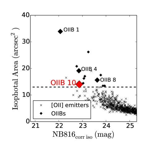
Figure 1.— Distribution of isophotal area and magnitudes in the ${\it{NB816_{\mathrm{corr}}}}$ image. The isophotal area criterion ($>13\ \mathrm{arcsec^{2}}$) is shown with the horizontal dashed line. The red diamond shows our target, OiiB 10. The black diamonds represent the rest of 11 OiiBs, and black crosses denote [Oii] emitters found by Drake et al. (2013). The two black crosses above the dashed line are [Oii] emitters that are not OiiBs, but objects with a large isophotal area made by source blending.

2.2. Multi-wavelength Imaging Data and Stellar Population of OiiB 10

Our target, OiiB 10, is covered by deep optical and infrared imaging data from several ground and space-based surveys: the Subaru XMM-Newton Deep Survey (SXDS; Furusawa et al. 2008), the UKIDSS Ultra Deep Survey (UDS; Lawrence et al. 2007; Warren et al. 2007), and the Spitzer public legacy survey of the UKIDSS UDS (SpUDS; PI: J. Dunlop). Figure 2 shows the multi-wavelength images of OiiB 10: the $BVRiz$ images from the SXDS, the $JHK$ images from the UKIDSS UDS, and the IRAC Ch1 ($3.6\ \mu$m), Ch2 ($4.5\ \mu$m), Ch3 ($5.8\ \mu$m), Ch4 ($8.0\ \mu$m) and MIPS $24\ \mu$m images from the SpUDS. We also present the $NB816_{\mathrm{corr}}$ and $Rz$ images produced by Y13. Although the Herschel SPIRE data are taken by the Herschel Multi-tiered Extragalactic Survey (HerMES; Oliver et al. 2012) in this field, the image of OiiB 10 is severely affected by source confusion. Hence, we do not use the SPIRE data.

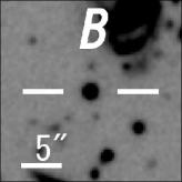
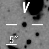
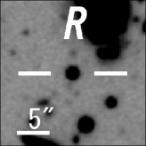
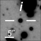
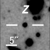
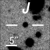
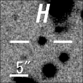
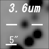
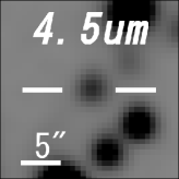
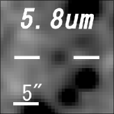
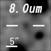
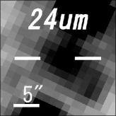
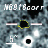
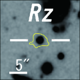
Figure 2.— Optical to mid-infrared images of OiiB 10. We display $20\arcsec\times 20\arcsec$ images at BVRizJHK, Spitzer/IRAC $3.6\ \mathrm{\mu m}$, $4.5\ \mathrm{\mu m}$, $5.8\ \mathrm{\mu m}$, $8.0\ \mathrm{\mu m}$, and Spitzer/MIPS $24\ \mathrm{\mu m}$ bands. We also show ${NB816_{\mathrm{corr}}}$ and ${\it Rz}$ images taken from Y13, which correspond to the [Oii] and continuum emission images, respectively. The $5\arcsec$ scale bar is plotted at the bottom left in each image. The yellow contours in the ${\it{NB816_{\mathrm{corr}}}}$ and ${\it Rz}$ images show the isophotal area above $2\sigma\ \mathrm{arcsec^{-2}}$ in the ${NB816_{\mathrm{corr}}}$ image as explained in Section 2.1.

The magnitudes in the $BVRiz$, $JHK$, $3.6\ \mu$m, and $4.5\ \mu$m bands are taken from Y13. In this study, we estimate the magnitudes of OiiB 10 in the $5.8\ \mathrm{\mu m}$, $8.0\ \mathrm{\mu m}$, and $24\ \mathrm{\mu m}$ bands. We obtain the magnitudes of the $5.8\ \mu$m and $8.0\ \mu$m bands with MAG_AUTO of SExtractor (Bertin & Arnouts 1996). The magnitude of the $24\ \mu$m band is estimated from galfit (Peng et al. 2002) modeling, since OiiB 10 is significantly blended with the three neighboring objects. We fit four objects, including OiiB 10, with PSF profiles whose flux amplitudes and positions are free parameters. Table 1 summarizes the magnitudes of OiiB 10 estimated from the multi-wavelength imaging data.

Table 1Magnitudes of OiiB 10

Band	Magunitude
$B$	$23.78\pm 0.02$
$V$	$23.42\pm 0.02$
$R$	$23.23\pm 0.02$
$i$	$22.90\pm 0.02$
$z$	$22.44\pm 0.03$
$J$	$22.05\pm 0.04$
$H$	$21.76\pm 0.04$
$K$	$21.39\pm 0.03$
$m(3.6\mathrm{\mu m})$	$20.98\pm 0.02$
$m(4.5\mathrm{\mu m})$	$21.09\pm 0.03$
$m(5.8\mathrm{\mu m})$	$21.6\pm 0.3$
$m(8.0\mathrm{\mu m})$	$21.9\pm 0.4$
$m(24\mathrm{\mu m})$	$19.0\pm 0.7$

Y13 have derived the stellar population properties of OiiB 10 by fitting model spectral energy distributions (SEDs) with the observed SED (see Figure 3 of Y13). The model SEDs have been constructed with the Bruzual & Charlot (2003) stellar population synthesis code. Y13 have assumed a constant star formation history, the Salpeter (1955) initial mass function (IMF) with lower and upper cutoff masses of 0.1 and 100 $M_{\odot}$, the dust attenuation law of Calzetti et al. (2000), and the solar metallicity. The SED fitting results are presented in Table 2. The color excess is $E(B-V)=0.31\pm 0.02$, implying that OiiB 10 is moderately dusty. The stellar age and the stellar mass are $270\pm 80\ \mathrm{Myr}$ and $(1.6\pm 0.2)\times 10^{10}\ M_{\odot}$, respectively. The SFR is ${\mathrm{SFR_{SED}}}=72\pm 8\ M_{\odot}\ \mathrm{yr^{-1}}$. Although we derive SFRs using different SFR indicators in Section 5.6, ${\mathrm{SFR_{SED}}}$ is our best estimate of OiiB 10’s SFR. This is because ${\mathrm{SFR_{SED}}}$ does not strongly depend on the metallicity but includes the extinction correction. The specific star formation rate (SSFR) is estimated to be high, $(45\pm 8)\times 10^{-10}\ \mathrm{yr}^{-1}$, suggesting that OiiB 10 is a starburst galaxy.

Table 2Stellar Population Properties of OiiB 10

Quantity	Value
$E(B-V)$	$0.31\pm 0.02\ \mathrm{mag}$
Stellar Age	$270\pm 80\ \mathrm{Myr}$
Stellar Mass	$1.6\pm 0.2\ \times 10^{10}\ M_{\odot}$
${\mathrm{SFR_{SED}}}$	$72\pm 8\ M_{\odot}\ \mathrm{yr}^{-1}$
${\mathrm{SFR}_{\textsc{[Oii]}}}$	$81\pm 27\ M_{\odot}\ \mathrm{yr}^{-1}$
${\mathrm{SFR_{H\beta}}}$	$96\pm 20\ M_{\odot}\ \mathrm{yr}^{-1}$
${\mathrm{SFR_{24\ {{\mu}m}}}}$	$100\pm 70\ M_{\odot}\ \mathrm{yr}^{-1}$

3. Observations and Data Analyses

3.1. MOSFIRE

We observed OiiB 10 with the MOSFIRE instrument (McLean et al. 2012) on the Keck-I telescope on 2013 October 8 (PI: M. Ouchi). A spectrum of OiiB 10 was obtained as a mask filler of this observation. We carried out $Y$-band spectroscopy, which covered the wavelength range of $9800$–$11000$ Å. Thus this observation targeted H$\beta$ and [Oiii]$\lambda\lambda 4959,5007$ lines redshifted to $z\sim 1.2$. The slit width was 0.$\!\!\arcsec$7. We used an ABAB dither pattern with individual exposures of 180 seconds. The total integration time was 2.4 hours, and the average seeing size was 0.$\!\!\arcsec$9 in an FWHM. The pixel scale was 0.$\!\!\arcsec$18 pixel^-1, and the spectral resolution was $R=3388$. We took the spectrum of a standard star, HIP 13917 (catalog ), for our flux calibration.

We reduce the data using the MOSFIRE data reduction pipeline. This pipeline performs flat fielding, wavelength calibration, sky subtraction, and cosmic ray removal before producing a combined two-dimensional spectrum for each slit. We then extract one-dimensional spectra from the two-dimensional reduced spectra using the iraf task apall. We sum the fluxes of 3.$\!\!\arcsec$24 ($18$ pixels) at each wavelength bin that covers about 95% of the emission.

To determine total line fluxes, we calculate a slit loss. Firstly, a radial profile of each line is estimated with the spatial distribution in the two-dimensional spectrum. We assume that the radial profile is identical in all directions, and calculate a correction factor to be 1.2. The $3\sigma$ limiting flux density is $\simeq 5\times 10^{-18}\ \mathrm{erg\ s^{-1}\ cm^{-2}\ \AA^{-1}}$ in the wavelength range of $9800-11000$ Å.

3.2. LDSS3

We conducted deep spectroscopic observations for OiiB 10 using the LDSS3 on the 6.5 m Magellan II (Clay) telescope on 2013 November 3 (PI: M. Rauch). We adopted a $0\farcs 8\times 3\farcs 5$ slitlet, and used the volume phase holographic (VPH)-red grism with the sloan-$i$ filter, which provided a spectral coverage between $6700$ and $8600$ Å. [Oii] lines redshifted to $z\sim 1.2$ were targeted in this configuration. In addition, we took spectra with the VPH-blue grism and the w4800–7800 filter, which covered the wavelength range from $4800$ Å to $6600$ Å. This configuration targeted metal absorption lines such as Mgii and Feii. The on-source exposure times with the VPH-red and VPH-blue configurations were $0.5$ hours ($=1\times 1800$ seconds) and $2.5$ hours ($=3\times 3000$ seconds), respectively. The average seeing size was $0\farcs 6$ in FWHM. The VPH-red (blue) grism had a spectral resolution of $R\sim 1710\ (1800)$. The LDSS3 instrument had a pixel scale of $0\farcs 189$ pixel^-1. Feige 110 (catalog ) was observed for our flux calibration.

The LDSS3 data are reduced by the Carnegie Observatories reduction package, cosmos. After bias subtraction, flat fielding, wavelength calibration, and rectification, one-dimensional spectra are extracted in the same manner as Section 3.1, except that the spectra are summed over 2.$\!\!\arcsec$27 ($12$ pixels) along the spatial axis to cover about 95% of the emission. We estimate a slit-loss correction factor to be 1.3 by the procedure same as Section 3.1. The $3\sigma$ flux density limit of the VPH-red spectrum is calculated to be $\simeq 8\times 10^{-18}\ \mathrm{erg\ s^{-1}\ cm^{-2}\ \AA^{-1}}$ in the wavelength range of $6700$–$8600$ Å.

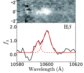
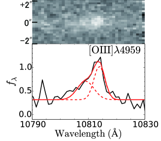
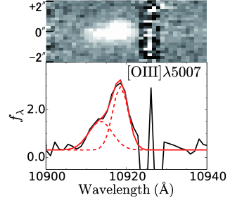
Figure 3.— MOSFIRE spectra of OiiB 10 at the wavelengths of H$\beta$ and [Oiii]$\lambda\lambda 4959,5007$ emission lines in the observed frame. The top panels present the two-dimensional spectra. In the bottom panels, the black solid lines indicate the observed spectra, and all emission lines show asymmetric profiles. The red solid lines denote the best-fit functions, and the red dashed lines represent Gaussian components of the best-fit functions. The units of the vertical axes are $10^{-17}\ \mathrm{erg\ s^{-1}\ cm^{-2}\ \AA^{-1}}$.

Table 3Emission Line Properties of OiiB 10.

Line	$z_{\mathrm{B}}\ /\ z_{\mathrm{R}}$	$f_{\mathrm{total}}^{\mathrm{corr}}$	$f_{\mathrm{total}}^{\mathrm{obs}}$	$f_{\mathrm{B}}^{\mathrm{obs}}$	$f_{\mathrm{R}}^{\mathrm{obs}}$	$\mathrm{FWHM}_{\mathrm{B}}\ /\ \mathrm{FWHM}_{\mathrm{R}}$
	(1)	(2)	(3)	(4)	(5)	(6)
[Oii]$\lambda 3726$	$1.1800\pm 0.0007$	$35.3\pm 11.6$	$6.5\pm 1.8$	…	…	$120\pm 60$
[Oii]$\lambda 3729$	$1.1800\pm 0.0007$	$37.5\pm 11.6$	$6.9\pm 1.8$	…	…	$120\pm 60$
$\mathrm{H\beta}$	$1.1794\pm 0.0004$ / $1.1807\pm 0.0007$	$53.2\pm 12.3$	$14.3\pm 2.6$	$3.5\pm 1.8$	$10.8\pm 1.9$	$70\pm 50$ / $130\pm 50$
[Oiii]$\lambda 4959$	$1.1797\pm 0.0007$ / $1.1806\pm 0.0005$	$26.9\pm 6.8$	$7.4\pm 1.5$	$3.4\pm 1.0$	$4.1\pm 1.0$	$120\pm 100$ / $100\pm 50$
[Oiii]$\lambda 5007$	$1.1797\pm 0.0007$ / $1.1806\pm 0.0005$	$90.2\pm 21.2$	$25.2\pm 4.5$	$10.3\pm 3.1$	$15.0\pm 3.1$	$120\pm 100$ / $100\pm 50$

Note. — All fluxes and FWHM line widths are in units of $\mathrm{10^{-17}\ erg\ s^{-1}cm^{-2}}$ and $\mathrm{km\ s^{-1}}$, respectively. All FWHM line widths are corrected for the instrumental broadening. Columns: (1) Redshifts for the blue ($z_{\mathrm{B}}$) and red ($z_{\mathrm{R}}$) components. (2) Total flux of two components after the slit-loss and dust-extinction corrections. (3) Total flux of the two components corrected only for the slit loss. (4)(5) Fluxes of blue $(f_{\mathrm{B}}^{\mathrm{obs}})$ and red $(f_{\mathrm{R}}^{\mathrm{obs}})$ components after the slit-loss correction. (6) FWHM line widths of the blue $(\mathrm{FWHM}_{\mathrm{B}})$ and red $(\mathrm{FWHM}_{\mathrm{R}})$ components.

4. Results

4.1. MOSFIRE

Figure 3 shows our MOSFIRE spectra at the wavelengths of [Oiii] and H$\beta$. We detect strong [Oiii] and H$\beta$ emission lines. These lines appear to have two components. We hereafter call the shorter-wavelength component ”the blue component”, and the longer-wavelength component ”the red component”. The red components appear to be spatially more extended than the blue components. The implications of these two-component profiles and the spatial extents are discussed in Section 5.9. The two-component H$\beta$ line is fitted with two Gaussian functions. The [Oiii] lines are the doublet lines, and each of the doublet lines has the blue and red components. Hence, we fit the [Oiii] lines with four Gaussian functions, assuming that each component of the [Oiii] doublet lines has the same line widths.

The results of the spectral line fittings are presented in Table 3. The redshift of the blue (red) component of [Oiii] lines is in agreement with that of the blue (red) component of H$\beta$ line within the $1\sigma$ uncertainties. We derive the average redshifts of the blue and red components to be $\left<z_{\mathrm{B}}\right>=1.1795\pm 0.0003$ and $\left<z_{\mathrm{R}}\right>=1.1806\pm 0.0004$, respectively, from the H$\beta$ and [Oiii] lines. The velocity difference derived from $\left<z_{\mathrm{B}}\right>$ and $\left<z_{\mathrm{R}}\right>$ is $170\pm 50\ \mathrm{km\ s^{-1}}$. The average redshift of all components is $z_{\mathrm{sys}}=1.1800\pm 0.0002$, and we define this average value as the systemic redshift of OiiB 10.

The estimated FWHM line widths are also summarized in Table 3. These FWHM line widths are corrected for the instrumental broadening on the assumption that their intrinsic profiles are Gaussian. The FWHM line widths of the [Oiii] lines are comparable to those of the H$\beta$ line within the $1\sigma$ uncertainties. The average FWHM line widths of blue and red components are $\left<\mathrm{FWHM_{B}}\right>=90\pm 50\ \mathrm{km\ s^{-1}}$ and $\left<\mathrm{FWHM_{R}}\right>=120\pm 40\ \mathrm{km\ s^{-1}}$, respectively.

We correct the fluxes for reddening by adopting the Calzetti et al. (2000) extinction law and $E(B-V)=0.31$ mag presented in Table 2. The fluxes after the dust-extinction correction are shown in Table 3.

4.2. LDSS3

Figure 4 presents our LDSS3 VPH-red grism spectrum at the wavelength of [Oii]. We identify [Oii] emission lines at the high significance level. In contrast to the MOSFIRE spectra of the H$\beta$ and [Oiii] lines, the LDSS3 spectrum of the [Oii] line does not show two components but one component. The non-detection of the blue and red components of the [Oii] doublet lines is due to the low resolution of the LDSS3 VPH-red data. The resolution of the LDSS3 VPH-red data ($R\sim 1710$) is lower than that of the MOSFIRE data ($R=3388$), and the velocity difference of $170\pm 50\ \mathrm{km\ s^{-1}}$ (Section 4.1) is not resolved in the LDSS3 data. Thus, each of the doublet lines has a one-component profile, and we fit [Oii] doublet lines with two Gaussian functions.

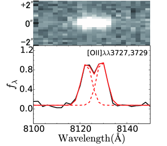
Figure 4.— LDSS3 spectrum of OiiB 10 taken with the VPH-red grism. Strong [Oii]$\lambda\lambda 3726,3729$ emission lines are detected. The top panel shows the two-dimensional spectrum. In the bottom panel, the black solid line shows the observed spectrum, and each of the doublet lines has a symmetric profile. The red solid line indicates the best-fit double Gaussian function, and the red dashed line represents each Gaussian component. The unit of the vertical axis is $10^{-17}\ \mathrm{erg\ s^{-1}\ cm^{-2}\ \AA^{-1}}$.

Table 3 summarizes the fitting results. The redshift of [Oii] doublet lines is consistent with the systemic redshift, $z_{\mathrm{sys}}=1.1800\pm 0.0002$. The [Oii] flux corrected for the slit loss is $f_{\mathrm{total}}^{\mathrm{obs}}$([Oii])$=(13.4\pm 5.1)\times 10^{-17}\ \mathrm{erg\ s^{-1}\ cm^{-2}\ \AA^{-1}}$, which is consistent with the [Oii] flux derived from the $NB816_{\mathrm{corr}}$ image, $14\times 10^{-17}\ \mathrm{erg\ s^{-1}\ cm^{-2}\ \AA^{-1}}$. The fluxes are corrected for the dust extinction in the same manner as Section 4.1.

Figure 5 indicates our LDSS3 VPH-blue grism spectra at the wavelengths of Mgii$\lambda\lambda$2796,2804 and Feii$\lambda\lambda$2587,2600. We identify Mgii$\lambda\lambda$2796,2804 and Feii$\lambda$2587 absorption lines at the 5.5 and 2.7 $\sigma$ levels, respectively. We do not examine the Feii$\lambda$2600 absorption line, since the sky background at this wavelength is relatively high. The Mgii$\lambda\lambda$2796,2804 and Feii$\lambda$2587 lines are fitted with two and one Gaussian function(s), respectively.

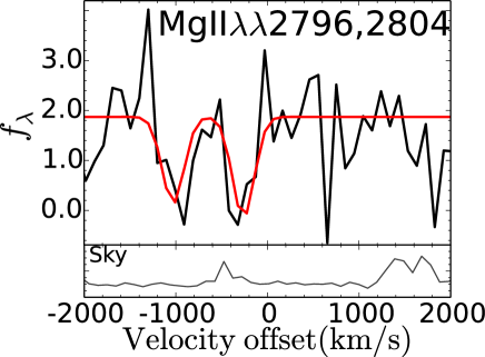
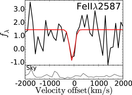
Figure 5.— LDSS3 spectra of OiiB 10 taken with the VPH-blue grism. The blueshifted Mgii$\lambda\lambda$2796,2804 (left panel) and Feii$\lambda$2587 (right panel) absorption lines are identified at the 5.5 and 2.7 $\sigma$ levels, respectively. In the top panels, black lines represent spectra of OiiB 10, and red lines denote the best-fit functions. The velocity offsets of Mgii$\lambda\lambda$2796,2804 and Feii$\lambda$2587 lines from the systemic velocity are $\Delta{v}=-260\pm 40$ km s^-1 and $\Delta{v}=-80\pm 50$ km s^-1, respectively. The bottom panels show the background sky spectra. The units of the vertical axes are arbitrary.

The fitting results are presented in Table 4. We find that the Mgii$\lambda\lambda$2796,2804 absorption lines are blueshifted from the systemic redshift by $|\Delta{v}|=260\pm 40$ km s^-1. The Feii$\lambda$2587 absorption line is also blueshifted, but the velocity offset is $|\Delta{v}|=80\pm 50$ km s^-1. Although the Feii$\lambda$2587 line is poorly identified, the velocity offset of the Feii$\lambda$2587 line may not be the same as that of the Mgii$\lambda\lambda$2796,2804 lines.

Table 4Absorption Line Properties of OiiB 10.

Line	$\mathrm{EW}$	$\Delta{v}$	$\mathrm{FWHM}$
	$\mathrm{(\AA)}$	($\mathrm{km\ s^{-1}}$)	($\mathrm{km\ s^{-1}}$)
	(1)	(2)	(3)
Mgii$\lambda$2796	$-2.6\pm 0.7$	$-260\pm 40$	$240\pm 110$
Mgii$\lambda$2803	$-3.1\pm 0.7$	$-260\pm 40$	$240\pm 110$
Feii$\lambda$2587	$-3.0\pm 1.1$	$-80\pm 50$	$180\pm 120$

Note. — Columns: (1) Rest-frame equivalent width. (2) Velocity offset from the systemic redshift. (3) FWHM line width corrected for the instrumental broadening.

5. Discussion

5.1. Signature of Outflow

In Section 4.2, we identify the Mgii$\lambda\lambda$2796,2804 and Feii$\lambda$2587 absorption lines blueshifted by $|\Delta{v}|=260\pm 40\ \mathrm{\mathrm{km\ s^{-1}}}$ and $|\Delta{v}|=80\pm 50$ km s^-1, respectively. These blueshifted absorption lines are evidence of outflows, because blueshifted photons are absorbed by the outflowing gas along the sight of the stars. From the blueshifted Mgii and Feii absorption lines, the outflow velocities are estimated to be $260\pm 40$ and $80\pm 50$ km s^-1, respectively. The difference of these outflow velocities may be significant; the implications of this difference are discussed in Section 5.3. Rupke et al. (2005a, b) suggest that outflow velocities of star-formation-driven (SF-driven) winds are $20-500\ \mathrm{\mathrm{km\ s^{-1}}}$, while those of galaxies hosting AGNs are $70-600\ \mathrm{\mathrm{km\ s^{-1}}}$. Thus, the low outflow velocity of OiiB 10, $80-260\ \mathrm{km\ s^{-1}}$, is comparable to those of AGN-driven winds as well as those of the SF-driven winds.

In some galaxy spectra, the Mgii line exhibits a P Cygni profile, which is composed of a redshifted resonance emission line on the intrinsic absorption trough (e.g., Martin & Bouché 2009; Weiner et al. 2009; Rubin et al. 2010, 2011; Prochaska et al. 2011; Coil et al. 2011; Erb et al. 2012; Martin et al. 2012, 2013). Rubin et al. (2011) detect Mgii doublet emission in a starburst galaxy at $z=0.69$ whose rest-frame EW is $3.6\ \mathrm{\AA}$. Assuming this EW, we can exclude the presence of the Mgii doublet emission in our LDSS3 VPH-blue data at the $3.6\ \sigma$ level. Weiner et al. (2009) suggest that the Mgii emission could be a weak AGN activity signature and/or backscattered light in the outflow. They report that blue and low-mass star-forming galaxies have Mgii emission lines stronger than red and high-mass star-forming galaxies. Martin et al. (2012) present the same trend, and suggest that this trend may be attributed to dust attenuation. Massive and red star-forming galaxies are dusty, and Mgii photons are absorbed by dust grains in the foreground gas. Thus, the non-detection of the Mgii emission line in our spectrum implies that OiiB 10 would be dusty.

5.2. Outflow Rate and Mass Loading Factor

Following the procedures of Rubin et al. (2010), we estimate the column density of the outflowing gas with the ratio of the Mgii doublet line EWs (see also Spitzer 1968; Jenkins 1986; Weiner et al. 2009). The EW ratio of the Mgii doublet lines, $\mathrm{EW}_{2796}/\mathrm{EW}_{2803}$, varies from 2 to 1 for optical depth, $\tau_{0}$, increasing from 0 to infinity. The Mg doublet EW ratio is approximately equal to $F(2\tau_{0})/F(\tau_{0})$, where $F(\tau_{0})$ is given by

$$F(\tau_{0})=\int_{0}^{\infty}(1-e^{-\tau_{0}\mathrm{exp}(-x^{2})})dx.$$ (1)

After the doublet ratio is estimated, we numerically derive $\tau_{0}$. Once $\tau_{0}$ is given, we calculate the column density in atoms, $N(\mathrm{Mg\textsc{ii}})$, using the equation from Spitzer (1968):

$$\begin{split}\mathrm{log}N(\mathrm{Mg\textsc{ii}})=\mathrm{log}\frac{|\mathrm{EW}_{2803}|}{\lambda}-\mathrm{log}\frac{2F(\tau_{0})}{\pi^{1/2}\tau_{0}}-\mathrm{log}\lambda{f_{2803}}\\ -\mathrm{log}C_{f}+20.053,\end{split}$$ (2)

where $\mathrm{log}\lambda{f_{2803}}=2.933$ and $C_{f}$ is the covering fraction. Here we assume $C_{f}=1$. The EW ratio, $\mathrm{EW}_{2796}/\mathrm{EW}_{2803}$, of OiiB 10 is $0.86\pm 0.30$, whose best-estimate value is smaller than unity. If we adopt the $1\sigma$ upper limit of the EW ratio, $\mathrm{EW}_{2796}/\mathrm{EW}_{2803}=1.16$, we obtain $\tau_{0}=5.9$, which corresponds to the $1\sigma$ lower limit. This $1\sigma$ lower limit yields $N(\mathrm{Mg\textsc{ii}})>4.9\times 10^{14}\ \mathrm{cm^{-2}}$. We assume $N(\mathrm{Mg\textsc{ii}})=N(\mathrm{Mg})$ and the abundance ratio of $\mathrm{log(Mg/H)}=-4.35$. The abundance ratio is derived from the metallicity of OiiB 10, $\mathrm{12+log[O/H]}=8.97$, estimated in Section 5.7. We adopt an Mg depletion onto dust of $-1.3$ dex, that is taken from Jenkins (2009) with an assumption of $n(\mathrm{H})\sim 1\ \mathrm{cm^{-3}}$. The column density of hydrogen is estimated to be $N(\mathrm{H})>2.2\times 10^{20}\ \mathrm{cm^{-2}}$. It should be noted that Equation (2) can be applied in the case of one absorbing cloud, but that this equation has also be shown to work adequately for the optical depth $\tau_{0}<5$. Because the calculated optical depth is $\tau_{0}>5.9$, this column density estimate would include some systemic uncertainties.

We calculate a mass outflow rate, $\dot{M}$, assuming a thin shell geometry. Weiner et al. (2009) give the mass outflow rate,

$$\dot{M}\simeq 22\ M_{\odot}\ \mathrm{yr}^{-1}C_{f}\frac{N(\mathrm{H})}{10^{20}\ \mathrm{cm^{-2}}}\frac{R}{5\ \mathrm{kpc}}\frac{v}{300\ \mathrm{km\ s^{-1}}},$$ (3)

where $R$ and $v$ are a radius of the shell wind and the outflow velocity, respectively. We adopt $R\sim 7.8\ \mathrm{kpc}$, which is the half of the spatial extent of the [Oii] emission in the $NB816_{\mathrm{corr}}$ image. If we take $v=220\pm 30\ \mathrm{km\ s^{-1}}$ that is the average of the outflow velocities derived from Mgii and Feii lines, the mass outflow rate is estimated to be $\dot{M}>55\pm 6\ M_{\odot}\ \mathrm{yr}^{-1}$. The error of the mass outflow rate only includes the uncertainty of the average outflow velocity.

A mass loading factor, $\eta$, characterizes a relation between a mass outflow rate and a SFR, and is defined as $\eta=\dot{M}/\mathrm{SFR}$. This mass loading factor serves as a critical function in models of galaxy evolution. Hopkins et al. (2012) predict mass loading factors of $0.5-2$ in SF-driven winds by the theoretical study. Observationally, the mass loading factors of AGNs and non-AGN U/LIRGs are estimated to be $\eta=0.1-1.1$ and $\eta=0.02-0.6$, respectively (Arribas et al. 2014, corrected for the Salpeter IMF). Rupke et al. (2005c) report the mass loading factors of starburst-dominated galaxies to be $\eta=0.01-1$. Using the mass outflow rate lower limit and the $\mathrm{SFR_{SED}}$, we estimate the mass loading factor of OiiB 10 to be $\eta>0.8\pm 0.1$. This mass loading factor is relatively high compared with those of the galaxies of Arribas et al. (2014) and Rupke et al. (2005c).

5.3. Difference of the Velocities of Mgii and Feii

The outflow velocities derived from Mgii and Feii absorption lines are $260\pm 40$ and $80\pm 50\ \mathrm{\mathrm{km\ s^{-1}}}$, respectively. Although this difference may not be true due to the marginal $2.7\sigma$ detection of the Feii line (Section 4.2), the difference of these two velocities could be explained by three possibilities. First possibility is the emission filling. As the Mgii transitions are resonantly trapped, these absorption lines are affected by filling from resonance emission lines. This resonance emission is generated by the foreground gas of the outflow. The resonance emission fills the absorption near the systemic redshift. This emission filling shifts the centroid of Mgii absorption to a bluer wavelength (e.g., Weiner et al. 2009; Kornei et al. 2012; Martin et al. 2012, 2013). However, we cannot conclude whether the emission filling occurs or not, because of the limited signal-to-noise ratio.

Second possibility is the difference of their oscillator strengths, as discussed in Kornei et al. (2012). Ionization potentials of Mg ($15.0\ \mathrm{eV}$) and Fe ($16.1\ \mathrm{eV}$) are nearly the same, while the oscillator strengths are different. The oscillator strength of the Mgii line at $2796\ \mathrm{\AA}$ ($f_{12}=0.60$) is larger than that of the Feii line at $2587\ \mathrm{\AA}$ ($f_{12}=0.07$). This difference indicates that Mgii is optically thick at a low density where Feii is optically thin. Because of the large cross-section for absorption, Mgii is a tracer of the low-density gas better than Feii. Note that such low-density gas is found far from galaxies, and that the speed of the galactic wind increases with increasing galactocentric radius (e.g Martin & Bouché 2009; Steidel et al. 2010; Dalla Vecchia & Schaye 2012). This physical picture explains that the velocity offset of Mgii absorption line is larger than that of Feii line.

Third possibility is the Feii absorption made by a foreground galaxy. In Section 4.1, we detect the two-component emission lines in our MOSFIRE spectrum. If OiiB 10 is a galaxy merger, the two components would correspond to two merging galaxies. The velocity offset of the blue component is $-70\pm 50\ \mathrm{km\ s^{-1}}$, comparable to that of the Feii absorption line. Hence, the Feii absorption could be made in the interstellar medium (ISM) of the foreground galaxy responsible for the blue component. On the other hand, the velocity offset of Mgii absorption lines is $\Delta v=-260\pm 40\ \mathrm{km\ s^{-1}}$, which is inconsistent with that of the blue component. This inconsistency implies that there is no strong Mgii absorption in the foreground galaxy, and that the Mgii absorption lines are made by the outflow of the major OiiB 10 galaxy. If it is true, an Mgii absorption of the foreground galaxy is absent, which is puzzling. However, it is possible that Mgii photons are scattered back into the line-of-sight from surrounding emission regions with no Mgii absorption.

5.4. Can the Outflowing Gas Escape from OiiB 10?

Comparing the outflow velocity with the local escape velocity, we examine whether the outflowing gas can escape from the gravitational potential of OiiB 10. Following the study of Weiner et al. (2009), we estimate the escape velocity, $v_{esc}$, at $r$ (see also Rubin et al. 2010; Martin et al. 2012). Under the assumption of a singular isothermal halo truncated at $r_{h}$, the escape velocity is

$$v_{esc}(r)=v_{c}\sqrt{2\left[1+\mathrm{ln}\left(\frac{r_{h}}{r}\right)\right]},$$ (4)

where $v_{c}$ is the circular velocity (Binney & Tremaine 1987). Although we do not have the $r_{h}/r$ estimate, this escape velocity very weakly depends on $r_{h}/r$. Assuming the plausible parameter range, $r_{h}/r=10-100$, we obtain $v_{esc}\simeq(2.6-3.3)v_{c}$. Thus the escape velocity is $v_{esc}\simeq(3.0\pm 0.4)v_{c}$. The relation between the circular velocity and the velocity dispersion, $\sigma$, of the [Oii] emission line is $\sigma\simeq(0.6\pm 0.1)v_{c}$ (Rix et al. 1997; Kobulnicky & Gebhardt 2000; Weiner et al. 2006). Combining this relation, we obtain the escape velocity of $v_{esc}\simeq(5\pm 1)\times\sigma$. Adopting the velocity dispersion of the [Oii] emission lines of OiiB 10, $\sigma=51\pm 26\ \mathrm{km\ s^{-1}}$, we calculate the escape velocity to be $v_{esc}=250\pm 140\ \mathrm{km\ s^{-1}}$. This escape velocity is comparable to the outflow velocity, $v=80-260\ \mathrm{km\ s^{-1}}$, implying that some fraction of the outflowing gas can escape from OiiB 10. Recently, the analytic models of Igarashi et al. (2014) predict the slowly accelerated outflows with increasing radius in the gravitational potential of a cold dark matter halo and a central super-massive black hole. Igarashi et al. (2014) apply their model to the Sombrero galaxy, and the model agrees with the radial density profile measured by observations. If the outflow is accelerated in OiiB 10 as claimed by Igarashi et al. (2014), more fraction of the gas would escape from OiiB 10. The escape of the outflowing gas indicates that the star formation activity may be suppressed in OiiB 10, and that the IGM would be chemically enriched by this outflow process.

5.5. Does OiiB 10 Have an AGN?

The next question is the energy source of the outflow of OiiB 10 that would be powered by an AGN activity and/or star formation. To examine the presence of the AGN, we search for a counterpart of OiiB 10 in the X-ray source catalog provided by Ueda et al. (2008). We find no detection within the circle of the X-ray positional error at the OiiB 10 position. It indicates that OiiB 10 does not harbor an X-ray luminous AGN with a $2-10\ \mathrm{keV}$ luminosity brighter than $10^{43}$ erg s^-1. However, we cannot rule out the possibility that OiiB 10 hosts a heavily obscured AGN with a faint X-ray luminosity.

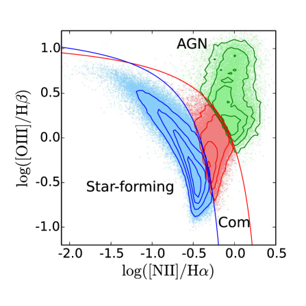
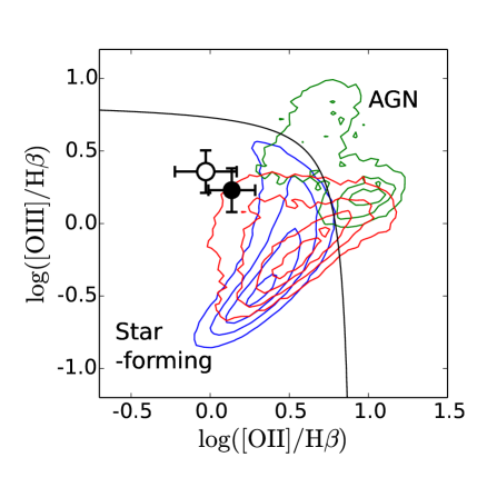
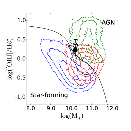
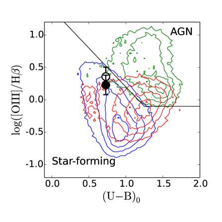
Figure 6.— BPT, blue, MEx, and CEx diagrams. The upper left panel shows the BPT diagram. We cannot plot OiiB 10 in the BPT diagram because the [Nii]$\lambda 6584$/H$\alpha$ ratio is not available in our study. Yet we use the BPT diagram to classify SDSS galaxies into pure star-forming galaxies, composites, and AGNs, in order to compare them with OiiB 10 in the blue, MEx, and CEx diagrams. The blue and red lines are boundaries of pure star-forming galaxies, composites, and AGNs, which are obtained by Kauffmann et al. (2003) and Kewley et al. (2001), respectively. The dots denote the SDSS galaxies. The pure star-forming galaxies, composites, and AGNs are shown with the dots and density contours of blue, red, and green colors, respectively. The upper right panel is the blue diagram. The black line is a boundary between pure star-forming galaxies and AGNs that is empirically determined by (Lamareille 2010). The lower left panel is the MEx diagram. The black lines are boundaries defined by Juneau et al. (2011). The lower right panel shows the CEx diagram. The black line is a boundary of Yan et al. (2011). In the blue, MEx, and CEx diagrams, OiiB 10 is shown with the black filled and open circles, which correspond to the extinction-corrected and uncorrected line ratios, respectively.

The BPT diagram (Baldwin et al. 1981) is the diagram of [Nii]$\lambda 6584$/H$\alpha$ vs. [Oiii]$\lambda 5007$/H$\beta$, which is widely used to distinguish AGNs and star-forming galaxies. The upper left panel of Figure 6 shows the BPT diagram. We plot SDSS galaxies taken from the data of SDSS DR7 (Abazajian et al. 2009). The blue and red classification lines are obtained from Kauffmann et al. (2003) and Kewley et al. (2001), respectively. We classify the SDSS galaxies based on this diagram. Galaxies that lie below the blue line are classified as pure star-forming galaxies. Galaxies located between the two classification lines are regarded as composites of an AGN and star-forming regions. Galaxies above the red line are classified as AGNs. The pure star-forming galaxies, composites, and AGNs are shown with the dots and contours of blue, red, and green colors, respectively. Because the [Nii]$\lambda 6584$ and H$\alpha$ lines of OiiB 10 are not covered by our spectroscopic data, we cannot plot OiiB 10 on the BPT diagram.

Instead of the BPT diagram, we adopt other three classification diagrams. The first is the diagram of the [Oii]$\lambda 3727/\mathrm{H\beta}$ and [Oiii]$\lambda 5007/\mathrm{H\beta}$ ratios (dubbed ”blue diagram”; e.g., Rola et al. 1997; Lamareille et al. 2004; Sobral et al. 2009; Lamareille 2010), which substitutes [Oii]$/\mathrm{H\beta}$ for [Nii]/H$\alpha$. The blue diagram is presented in the upper right panel of Figure 6, and the empirical boundary between pure star-forming galaxies and AGNs (Lamareille 2010) is shown with the black line. The second is called the mass-excitation diagram (MEx diagram; Juneau et al. 2011), which utilizes the stellar mass instead of [Nii]/H$\alpha$. The lower left panel in Figure 6 is the MEx diagram with the boundaries in the black lines defined by Juneau et al. (2011). It should be noted that the boundaries are not well calibrated at $z\gtrsim 1$. The third is the color-excitation diagram (CEx diagram; Yan et al. 2011), which uses the rest-frame $U-B$ color in place of [Nii]/H$\alpha$. The CEx diagram is shown in the lower right panel. The black line indicates the boundary defined by Yan et al. (2011). In these three diagrams, contours of the pure star-forming galaxies, composites, and AGNs are plotted with the colors same as the BPT diagram.

In the blue, MEx, and CEx diagrams, OiiB 10 is denoted by the red circles. In the blue diagram, we find that OiiB 10 lies in the composite region. In the MEx diagram, OiiB 10 is located not only in the composite region, but also on the edge of the AGN or the pure star-forming galaxy regions. In the CEx diagram, OiiB 10 lies on the edge of the AGN or the composite regions, as well as in the pure star-forming region. While it is likely that OiiB 10 is a composite of an AGN and star-forming regions from these three diagrams, the possibilities of an AGN and a pure star-forming galaxy still remain.

As described in Section 4, the FWHM emission line widths of OiiB 10 are narrow, $70-130\ \mathrm{km\ s^{-1}}$. It is widely known that type-1 AGNs have spectra with very broad permitted lines whose FWHM line widths are $\simeq(1-5)\times 10^{3}\ \mathrm{km\ s^{-1}}$, and with moderately broad ($\sim 500\ \mathrm{km\ s^{-1}}$) forbidden lines such as [Oiii]$\lambda\lambda 4959,5007$. The typical FWHM emission line width of type-2 AGNs is $500\ \mathrm{km\ s^{-1}}$, which is similar to those of the forbidden lines in type-1 AGNs. Yet Kewley et al. (2006) report that the FWHM emission line widths of type-2 AGNs and composites are $100-600\ \mathrm{km\ s^{-1}}$. Star-forming galaxies typically show line widths narrower than those of AGNs (Osterbrock 1989). Although the narrow line widths of OiiB 10 generally imply that OiiB 10 would be a star-forming galaxy, these line widths are consistent with those of some type-2 AGNs and composites.

5.6. Stellar Population of OiiB 10

The multi-wavelength SED of OiiB 10 is shown in Figure 7. Figure 7 compares the SED of OiiB 10 with those of local starburst templates (Silva et al. 1998). The mid-infrared SED shape of OiiB 10 is similar to those of Arp220 (catalog ), NGC6090 (catalog ), and M82 (catalog ). This indicates that OiiB 10 is a dusty starburst galaxy, consistent with the non-detection of the Mgii emission line discussed in Section 5.1.

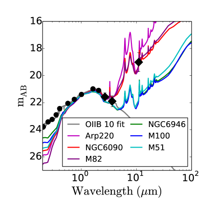
Figure 7.— SED of OiiB 10 in the rest frame wavelength. The black diamonds represent the magnitudes obtained in this study, and the black circles show the magnitudes estimated in Y13. The gray line is the result of the SED fitting in Y13. The magenta, red, purple, green, blue, and cyan lines indicate the SEDs of Arp220, NGC6090, M82, NGC6946, M100, and M51 (Silva et al. 1998), respectively. All SEDs are normalized at the $K$ band magnitude. The mid-infrared SED shape of OiiB 10 is similar to those of the local dusty starbursts, Arp220, NGC6090, and M82, suggesting that the OiiB 10 is a dusty starburst galaxy.

We calculate the SFR of OiiB 10 using the [Oii] or H$\beta$ emission line luminosity with the formulae of Kennicutt (1998). We estimate the $\mathrm{H\alpha}$ luminasity from our extinction-corrected $\mathrm{H\beta}$ luminosity with the line ratio of $L(\mathrm{H\alpha}):L(\mathrm{H\beta})=2.86:1$, under the assumption of Case B recombination in a nebula with a temperature of $T=10000\ \mathrm{K}$ and an electron density of $n_{e}=100\ \mathrm{cm^{-3}}$ (Osterbrock 1989). The SFRs derived from the [Oii] and $\mathrm{H\beta}$ luminosities are ${\mathrm{SFR}_{\textsc{[Oii]}}}=81\pm 27$ and ${\mathrm{SFR}_{H\beta}}=96\pm 20\ M_{\odot}\ \mathrm{yr}^{-1}$, respectively. They are consistent with the SFR from the SED fitting, ${\mathrm{SFR_{SED}}}=72\pm 8\ M_{\odot}\ \mathrm{yr}^{-1}$. We also estimate the SFR with our MIPS $24\ \mathrm{\mu m}$ flux. Following the equations in Rieke et al. (2009), we obtain ${\mathrm{SFR_{24\ {{\mu}m}}}}=100\pm 70\ M_{\odot}\ \mathrm{yr}^{-1}$. These SFRs are summarized in Table 2. The SSFR of OiiB 10  derived from the [Oii] or H$\beta$ luminosities is $(45-60)\times 10^{-10}\ \mathrm{yr}^{-1}$. This SSFR is higher than those of Arp220 (catalog ), NGC6090 (catalog ), and M82 (catalog ), that are $25$, $1.7$ and $3.1\ \times 10^{-10}\ \mathrm{yr}^{-1}$, respectively (Silva et al. 1998).

5.7. Metallicity and Ionization Parameter

In this Section, we examine the metal abundance and ionization state of the ISM in OiiB 10. For simplicity, we assume that OiiB 10 is dominated by the starburst, and adopt photoionization models. The $R23$-index and the ratio of [Oiii]$\lambda 5007$ to [Oii]$\lambda 3727$ ([Oiii]/[Oii] ratio) are useful for investigating metallicities, $\mathrm{12+log(O/H)}$, and ionization parameters, $q_{\mathrm{ion}}$, of galaxies (Kewley & Dopita 2002; Nakajima et al. 2013; Nakajima & Ouchi 2013). The $R23$-index and [Oiii]/[Oii] ratio of OiiB 10 are $R_{23}=3.57\pm 0.99$ and $\mathrm{{\textsc{[Oiii]}}/{\textsc{[Oii]}}}=1.24\pm 0.40$, respectively. Figure 8 shows the diagram of $R23$-index vs. [Oiii]/[Oii] ratio, and OiiB 10 is denoted by a red circle. The black solid (dashed) curves indicate photoionization model tracks with the constant ionization parameters (metallicities). These model tracks are calculated with the formulae presented in Kewley & Dopita (2002). The SDSS galaxies are plotted with the gray dots. The red diamonds and the blue triangles represent $z>2$ and $0.5<z<2$ galaxies, respectively, that are compiled by Nakajima & Ouchi (2013). As shown in Figure 8, the $R_{23}$ value and the [Oiii]/[Oii] ratio of OiiB 10 are comparable to those of the $0.5<z<2$ galaxies.

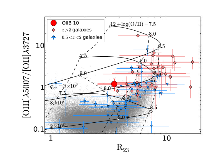
Figure 8.— $R23$-index vs. [Oiii]$\lambda 5007$/[Oii]$\lambda 3727$ diagram. The red circle denotes OiiB 10. The gray dots represent the SDSS galaxies. The red diamonds and the blue triangles indicate $z>2$ and $0.5<z<2$ galaxies, respectively, that are compiled by Nakajima & Ouchi (2013). The $R_{23}$ and the [Oiii]/[Oii] values of OiiB 10 are comparable to those of the $0.5<z<2$ galaxies. The black solid curves show the photoionization model tracks with ionization parameters of $q_{\mathrm{ion}}=0.2,0.8,\mathrm{and}\ 3\times 10^{8}\ \mathrm{cm\ s^{-1}}$, for the metallicity range of $\mathrm{12+log(O/H)}=7.5-9.5$. The dashed lines indicate the constant metallicities of $\mathrm{12+log(O/H)}=7.5,8.0,8.5,\mathrm{and}\ 9.0$. These model tracks are calculated with the formulae presented in Kewley & Dopita (2002).

Following the equations in Kobulnicky & Kewley (2004), we estimate the metallicity and ionization parameter of OiiB 10 from the $R23$-index and [Oiii]/[Oii] ratio. There are two solutions: $(\mathrm{12+log[O/H]},\ q_{\mathrm{ion}}[10^{8}\ \mathrm{cm\ s^{-1}}])$ $=$ $(8.97\pm 0.08,\ 1.3\pm 0.7)$ and $(7.87\pm 0.19,\ 0.32\pm 0.08)$, which are high and low metallicity solutions, respectively. The SED fitting results presented in Section 2.2 reveal that the stellar mass of OiiB 10 is relatively high, $1.6\times 10^{10}\ M_{\odot}$. We assume that this high stellar mass is due to the past star formation that largely contributes to the metal enrichment of ISM. Moreover, as discussed in Section 5.6, OiiB 10 is a dusty starburst galaxy. Thus, OiiB 10 should have the high-metallicity solution, $(\mathrm{12+log[O/H]},\ q_{\mathrm{ion}}[10^{8}\ \mathrm{cm\ s^{-1}}])$ $=$ $(8.97\pm 0.08,\ 1.3\pm 0.7)$, which indicates the high ionization parameter. The ionization parameter of OiiB 10 is comparable to those of the $z>2$ galaxies. However, the metallicity of OiiB 10 is significantly higher than those of the $z>2$ galaxies, and similar to those of SDSS metal-rich galaxies in Figure 8.

5.8. Comparison with Other Galaxies

We compare the properties of OiiB 10 with those of other OiiBs. Y13 study OiiB 1, 4, and 8 with the optical spectroscopic data, and find that OiiB 1 and 4 have outflow signatures. The outflow velocity of OiiB 10 is comparable to that of OiiB 4 ($\sim\ 200\ \mathrm{\mathrm{km\ s^{-1}}}$), and much less than that of OiiB 1 ($500-600\ \mathrm{\mathrm{km\ s^{-1}}}$) that exhibits the AGN activity. Mgii$\lambda\lambda$2796,2804 and Feii$\lambda$2587 absorption lines, which are found in OiiB 10, are also detected in OiiB 4. In OiiB 1, however, only the Feii$\lambda$2587 absorption line is marginally detected. These facts imply that the outflow mechanism of OiiB 10 may be similar to that of OiiB 4. The ionization parameter of OiiB 10 is $q_{\mathrm{ion}}=(1.3\pm 0.7)\times 10^{8}\ \mathrm{cm\ s^{-1}}$, corresponding to $\mathrm{log}U=-2.36\pm 0.26$. This ionization parameter is lower than that of OiiB 1, $\mathrm{log}U>-1.0$, which is estimated from the [Oii]$\lambda 3727$/Feii^∗$\lambda 2613$ ratio.

Then, we compare OiiB 10 with typical star-forming galaxies at $z\sim 1.5$ and $2.2$. Masters et al. (2014, hereafter M14) study the emission line galaxies at $z\sim 1.5$ and $2.2$ with near-infrared spectroscopic data. Their galaxies have strong [Oiii] and/or H$\alpha$ emission lines. Thus, the average spectrum of these galaxies in M14 represents the typical star-forming galaxies. The [Oiii] line width of OiiB 10 presented in Table 3 is comparable to that of the average spectrum in M14, $75\ \mathrm{\mathrm{km\ s^{-1}}}$. The ionization parameter of OiiB 10, $\mathrm{log}U=-2.36\pm 0.26$, is also simililar to that of the average spectrum in M14, $\mathrm{log}U=-2.49^{+0.07}_{-0.14}$. However, the metallicity of OiiB 10, $\mathrm{12+log[O/H]}=8.97\pm 0.08$, is higher than that of the average spectrum in M14, $\mathrm{12+log[O/H]}=8.37$. This indicates that OiiB 10 is more metal-rich than the typical star-forming galaxies at $z\sim 1.5$ and $2.2$.

5.9. What is OiiB 10?

We discuss the physical origin of OiiB 10. As described in Section 4.1, we identify the two-components emission lines in OiiB 10, and the red components appear to be spatially more extended than the blue components. The origin of the two components is unknown, but there are three possibilities: (1) two strong star-forming regions, (2) a galaxy merger, and (3) a combination of a galaxy and an outflow knot. The first possibility is that OiiB 10 has two strong star-forming regions, which make the two emission line components. The velocity difference of the two components ($170\pm 50\ \mathrm{km\ s^{-1}}$) may be due to a rotation or an infall of these two star-forming regions. The second possibility is that the OiiB 10 is a merger system, and that the two components correspond to the two galaxies. When galaxies merge, large amounts of the ISM fall on the central regions. This leads to the starburst processes. As discussed in Section 5.6, OiiB 10 is a dusty starburst galaxy, which supports this merger-triggered starburst scenario. Generally, merging galaxies have broad ($v_{\mathrm{FWHM}}\agt 350\ \mathrm{km\ s^{-1}}$) and narrow ($v_{\mathrm{FWHM}}\alt 350\ \mathrm{km\ s^{-1}}$) emission lines that are produced by a shocked gas and Hii regions, respectively (e.g., Rich et al. 2011; Soto et al. 2012; Rupke & Veilleux 2013). However, we do not detect broad lines in OiiB 10. The non-detection of the broad lines implies that the shock excitation would not be dominant in OiiB 10. The third possibility is that Hii regions and one collimated outflow knot of the ionized gas are responsible for the two components, respectively. As discussed in Section 5.1, OiiB 10 has the outflow. If the outflow is beamed to us, the faint blue component of the emission line would be the outflow knot. In this case, the bright red component is originated from the Hii regions. The outflow velocity should be comparable to the velocity difference of the two emission line components, $170\pm 50\ \mathrm{\mathrm{km\ s^{-1}}}$ (Section 4.1). With $z_{\mathrm{R}}$ and the absorption line velocities, we estimate the outflow velocity for the red component to be $160-390\ \mathrm{km\ s^{-1}}$, comparable to the velocity difference of the two components. None of these three possibilities can be conclusively ruled out given current observational results including the fact that the red components appear to be more extended than the blue components.

The next question of OiiB 10 is the energy source of the outflow found in Section 5.1. From the diagrams of Figure 6, it is likely that OiiB 10 is a composite of an AGN and star-forming regions. The narrow emission line widths of OiiB 10, $70-130\ \mathrm{km\ s^{-1}}$ (Section 4), are comparable not only to star-forming galaxies but also to type-2 AGNs and composites. Thus a type-2 AGN and star formation would drive the outflow of OiiB 10. For further investigation of the outflow and the presence of an AGN, observations with adaptive optics (AO) would be needed.

6. Summary

We present the Keck/MOSFIRE and Magellan/LDSS3 spectroscopy and the archival imaging data of thirteen bands for the object with the spatially extended [Oii]$\lambda\lambda 3726,3729$ emission at $z=1.18$, [Oii] blob 10 (OiiB 10). Following the study of Yuma et al. (2013), our data provide new insight into the physical properties of OiiB 10. This is the first detailed spectroscopic study of oxygen-line blobs which includes the analyses of the escape velocity, the mass loading factor, and the presence of an AGN, and is a significant step for understanding the nature of oxygen-line blobs and the relationship between gas outflow and star formation quenching at high redshift. The major results of our study are summarized below.

1. By our MOSFIRE observations, we identify H$\beta$ and [Oiii]$\lambda\lambda 4959,5007$ emission lines, all of which show the profiles of the two components that are called blue and red components. The average redshift of all components is $z_{\mathrm{sys}}=1.1800\pm 0.0002$, which is defined as the systemic redshift of OiiB 10. The velocity difference of the blue and red components is $170\pm 50\ \mathrm{km\ s^{-1}}$. We estimate the average FWHM line widths of the blue and red components to be $\mathrm{FWHM_{B}}=90\pm 50\ \mathrm{km\ s^{-1}}$ and $\mathrm{FWHM_{R}}=120\pm 40\ \mathrm{km\ s^{-1}}$, respectively.

2. We detect [Oii]$\lambda\lambda 3726,3729$ emission lines in our LDSS3 VPH-red grism spectrum. Although we identify the doublet lines of [Oii], the blue and red components are not resolved in our spectrum. The redshift of [Oii] lines is $z=1.1800\pm 0.0007$, consistent with the systemic redshift. The FWHM line width is estimated to be $120\pm 60\ \mathrm{km\ s^{-1}}$.

3. In our LDSS3 VPH-blue grism spectrum, we identify blueshifted Mgii$\lambda\lambda$2796,2804 and Feii$\lambda$2587 absorption lines. The velocity offsets from the systemic velocity are $\Delta{v}=-260\pm 40\ \mathrm{\mathrm{km\ s^{-1}}}$ and $\Delta{v}=-80\pm 50\ \mathrm{km\ s^{-1}}$ for the Mgii and Feii absorption lines, respectively. These blueshifted absorption lines indicate that OiiB 10 has an outflow whose velocity is $80-260\ \mathrm{km\ s^{-1}}$.

4. The escape velocity of OiiB 10 is estimated to be $v_{esc}=250\pm 140\ \mathrm{km\ s^{-1}}$. The outflow velocity of OiiB 10, $80-260\ \mathrm{km\ s^{-1}}$, is comparable to this escape velocity, implying that some fraction of the outflowing gas would escape from OiiB 10. This indicates that the star formation activity could be suppressed by the outflow, and that the chemical enrichment of IGM may take place.

5. To examine the presence of the AGN, we investigate line ratios, the stellar mass, and the color with the ”blue”, MEx, and CEx diagrams. These diagrams indicate that OiiB 10 would be a composite of an AGN and star-forming regions, but do not rule out the possibilities of an AGN and a pure star-forming galaxy. While the narrow line widths of OiiB 10 are suggestive of a star-forming galaxy, they are also consistent with an AGN or a composite.

6. The SED of OiiB 10 suggests that OiiB 10 is a dusty starburst galaxy, because the mid-infrared SED shape is similar to those of local starburst galaxies. We estimate the metallicity and ionization parameter of OiiB 10 to be $\mathrm{12+log(O/H)}=8.97\pm 0.08$ and $q_{\mathrm{ion}}=(1.3\pm 0.7)\times 10^{8}\ \mathrm{cm\ s^{-1}}$, respectively.

7. The two-component emission lines found in our MOSFIRE spectrum would indicate three possibilities: (1) two strong star-forming regions, (2) a galaxy merger, and (3) a combination of a galaxy and an outflow knot. These three possibilities are all consistent with the results from our observations. The outflow may be driven by a composite of star formation and a type-2 AGN.

References

- Abazajian et al. (2009) Abazajian, K. N., Adelman-McCarthy, J. K., Agüeros, M. A., et al. 2009, ApJS, 182, 543
- Arribas et al. (2014) Arribas, S., Colina, L., Bellocchi, E., Maiolino, R., & Villar-Martin, M. 2014, ArXiv e-prints, arXiv:1404.1082
- Baldwin et al. (1981) Baldwin, J. A., Phillips, M. M., & Terlevich, R. 1981, PASP, 93, 5
- Baugh (2006) Baugh, C. M. 2006, Reports on Progress in Physics, 69, 3101
- Bertin & Arnouts (1996) Bertin, E., & Arnouts, S. 1996, A&AS, 117, 393
- Binney & Tremaine (1987) Binney, J., & Tremaine, S. 1987, Galactic dynamics
- Bower et al. (2004) Bower, R. G., Morris, S. L., Bacon, R., et al. 2004, MNRAS, 351, 63
- Bruzual & Charlot (2003) Bruzual, G., & Charlot, S. 2003, MNRAS, 344, 1000
- Calzetti et al. (2000) Calzetti, D., Armus, L., Bohlin, R. C., et al. 2000, ApJ, 533, 682
- Clarke & Oey (2002) Clarke, C., & Oey, M. S. 2002, MNRAS, 337, 1299
- Coil et al. (2011) Coil, A. L., Weiner, B. J., Holz, D. E., et al. 2011, ApJ, 743, 46
- Colbert et al. (2006) Colbert, J. W., Teplitz, H., Francis, P., et al. 2006, ApJ, 637, L89
- Cole et al. (2000) Cole, S., Lacey, C. G., Baugh, C. M., & Frenk, C. S. 2000, MNRAS, 319, 168
- Dalla Vecchia & Schaye (2012) Dalla Vecchia, C., & Schaye, J. 2012, MNRAS, 426, 140
- Dekel & Birnboim (2006) Dekel, A., & Birnboim, Y. 2006, MNRAS, 368, 2
- Dey et al. (2005) Dey, A., Bian, C., Soifer, B. T., et al. 2005, ApJ, 629, 654
- Dijkstra et al. (2006) Dijkstra, M., Haiman, Z., & Spaans, M. 2006, ApJ, 649, 37
- Dijkstra & Kramer (2012) Dijkstra, M., & Kramer, R. 2012, MNRAS, 424, 1672
- Dijkstra & Loeb (2009) Dijkstra, M., & Loeb, A. 2009, MNRAS, 400, 1109
- Dove et al. (2000) Dove, J. B., Shull, J. M., & Ferrara, A. 2000, ApJ, 531, 846
- Drake et al. (2013) Drake, A. B., Simpson, C., Collins, C. A., et al. 2013, MNRAS, 433, 796
- Erb et al. (2012) Erb, D. K., Quider, A. M., Henry, A. L., & Martin, C. L. 2012, ApJ, 759, 26
- Erb et al. (2006) Erb, D. K., Shapley, A. E., Pettini, M., et al. 2006, ApJ, 644, 813
- Fardal et al. (2001) Fardal, M. A., Katz, N., Gardner, J. P., et al. 2001, ApJ, 562, 605
- Francis et al. (2001) Francis, P. J., Williger, G. M., Collins, N. R., et al. 2001, ApJ, 554, 1001
- Fujita et al. (2003) Fujita, A., Martin, C. L., Mac Low, M.-M., & Abel, T. 2003, ApJ, 599, 50
- Furusawa et al. (2008) Furusawa, H., Kosugi, G., Akiyama, M., et al. 2008, ApJS, 176, 1
- Fynbo et al. (1999) Fynbo, J. U., Møller, P., & Warren, S. J. 1999, MNRAS, 305, 849
- Geach et al. (2009) Geach, J. E., Alexander, D. M., Lehmer, B. D., et al. 2009, ApJ, 700, 1
- Gnedin et al. (2008) Gnedin, N. Y., Kravtsov, A. V., & Chen, H.-W. 2008, ApJ, 672, 765
- Goerdt et al. (2010) Goerdt, T., Dekel, A., Sternberg, A., et al. 2010, MNRAS, 407, 613
- Haiman et al. (2000) Haiman, Z., Spaans, M., & Quataert, E. 2000, ApJ, 537, L5
- Hashimoto et al. (2013) Hashimoto, T., Ouchi, M., Shimasaku, K., et al. 2013, ApJ, 765, 70
- Hayes et al. (2011) Hayes, M., Scarlata, C., & Siana, B. 2011, Nature, 476, 304
- Heckman et al. (1997) Heckman, T. M., Gonzalez-Delgado, R., Leitherer, C., et al. 1997, ApJ, 482, 114
- Heckman et al. (2000) Heckman, T. M., Lehnert, M. D., Strickland, D. K., & Armus, L. 2000, ApJS, 129, 493
- Heckman et al. (2002) Heckman, T. M., Norman, C. A., Strickland, D. K., & Sembach, K. R. 2002, ApJ, 577, 691
- Heckman et al. (2001a) Heckman, T. M., Sembach, K. R., Meurer, G. R., et al. 2001a, ApJ, 558, 56
- Heckman et al. (2001b) —. 2001b, ApJ, 554, 1021
- Heckman et al. (2011) Heckman, T. M., Borthakur, S., Overzier, R., et al. 2011, ApJ, 730, 5
- Hopkins et al. (2012) Hopkins, P. F., Quataert, E., & Murray, N. 2012, MNRAS, 421, 3522
- Igarashi et al. (2014) Igarashi, A., Mori, M., & Nitta, S.-y. 2014, ArXiv e-prints, arXiv:1405.3978
- Jeeson-Daniel et al. (2012) Jeeson-Daniel, A., Ciardi, B., Maio, U., et al. 2012, MNRAS, 424, 2193
- Jenkins (1986) Jenkins, E. B. 1986, ApJ, 304, 739
- Jenkins (2009) —. 2009, ApJ, 700, 1299
- Jones et al. (2012) Jones, T., Stark, D. P., & Ellis, R. S. 2012, ApJ, 751, 51
- Juneau et al. (2011) Juneau, S., Dickinson, M., Alexander, D. M., & Salim, S. 2011, ApJ, 736, 104
- Kauffmann et al. (2003) Kauffmann, G., Heckman, T. M., Tremonti, C., et al. 2003, MNRAS, 346, 1055
- Kennicutt (1998) Kennicutt, Jr., R. C. 1998, ARA&A, 36, 189
- Kereš et al. (2009) Kereš, D., Katz, N., Davé, R., Fardal, M., & Weinberg, D. H. 2009, MNRAS, 396, 2332
- Kewley & Dopita (2002) Kewley, L. J., & Dopita, M. A. 2002, ApJS, 142, 35
- Kewley et al. (2001) Kewley, L. J., Dopita, M. A., Sutherland, R. S., Heisler, C. A., & Trevena, J. 2001, ApJ, 556, 121
- Kewley et al. (2006) Kewley, L. J., Groves, B., Kauffmann, G., & Heckman, T. 2006, MNRAS, 372, 961
- Kobulnicky & Gebhardt (2000) Kobulnicky, H. A., & Gebhardt, K. 2000, AJ, 119, 1608
- Kobulnicky & Kewley (2004) Kobulnicky, H. A., & Kewley, L. J. 2004, ApJ, 617, 240
- Kornei et al. (2012) Kornei, K. A., Shapley, A. E., Martin, C. L., et al. 2012, ApJ, 758, 135
- Lamareille (2010) Lamareille, F. 2010, A&A, 509, A53
- Lamareille et al. (2004) Lamareille, F., Mouhcine, M., Contini, T., Lewis, I., & Maddox, S. 2004, MNRAS, 350, 396
- Laursen & Sommer-Larsen (2007) Laursen, P., & Sommer-Larsen, J. 2007, ApJ, 657, L69
- Lawrence et al. (2007) Lawrence, A., Warren, S. J., Almaini, O., et al. 2007, MNRAS, 379, 1599
- Leauthaud et al. (2012) Leauthaud, A., Tinker, J., Bundy, K., et al. 2012, ApJ, 744, 159
- Lequeux et al. (1995) Lequeux, J., Kunth, D., Mas-Hesse, J. M., & Sargent, W. L. W. 1995, A&A, 301, 18
- Martin (2005) Martin, C. L. 2005, ApJ, 621, 227
- Martin & Bouché (2009) Martin, C. L., & Bouché, N. 2009, ApJ, 703, 1394
- Martin et al. (2012) Martin, C. L., Shapley, A. E., Coil, A. L., et al. 2012, ApJ, 760, 127
- Martin et al. (2013) —. 2013, ApJ, 770, 41
- Masters et al. (2014) Masters, D., McCarthy, P., Siana, B., et al. 2014, ArXiv e-prints, arXiv:1402.0510
- Matsuda et al. (2004) Matsuda, Y., Yamada, T., Hayashino, T., et al. 2004, AJ, 128, 569
- Matsuda et al. (2011) —. 2011, MNRAS, 410, L13
- McLean et al. (2012) McLean, I. S., Steidel, C. C., Epps, H. W., et al. 2012, in Society of Photo-Optical Instrumentation Engineers (SPIE) Conference Series, Vol. 8446, Society of Photo-Optical Instrumentation Engineers (SPIE) Conference Series
- Momose et al. (2014) Momose, R., Ouchi, M., Nakajima, K., et al. 2014, ArXiv e-prints, arXiv:1403.0732
- Mori et al. (2004) Mori, M., Umemura, M., & Ferrara, A. 2004, ApJ, 613, L97
- Murray et al. (2011) Murray, N., Ménard, B., & Thompson, T. A. 2011, ApJ, 735, 66
- Murray et al. (2005) Murray, N., Quataert, E., & Thompson, T. A. 2005, ApJ, 618, 569
- Nakajima & Ouchi (2013) Nakajima, K., & Ouchi, M. 2013, ArXiv e-prints, arXiv:1309.0207
- Nakajima et al. (2013) Nakajima, K., Ouchi, M., Shimasaku, K., et al. 2013, ApJ, 769, 3
- Nilsson et al. (2006) Nilsson, K. K., Fynbo, J. P. U., Møller, P., Sommer-Larsen, J., & Ledoux, C. 2006, A&A, 452, L23
- Ohyama & Taniguchi (2004) Ohyama, Y., & Taniguchi, Y. 2004, AJ, 127, 1313
- Ohyama et al. (2003) Ohyama, Y., Taniguchi, Y., Kawabata, K. S., et al. 2003, ApJ, 591, L9
- Oliver et al. (2012) Oliver, S. J., Bock, J., Altieri, B., et al. 2012, MNRAS, 424, 1614
- Osterbrock (1989) Osterbrock, D. E. 1989, Astrophysics of gaseous nebulae and active galactic nuclei
- Ouchi et al. (2009) Ouchi, M., Ono, Y., Egami, E., et al. 2009, ApJ, 696, 1164
- Overzier et al. (2013) Overzier, R. A., Nesvadba, N. P. H., Dijkstra, M., et al. 2013, ApJ, 771, 89
- Palunas et al. (2004) Palunas, P., Teplitz, H. I., Francis, P. J., Williger, G. M., & Woodgate, B. E. 2004, ApJ, 602, 545
- Peng et al. (2002) Peng, C. Y., Ho, L. C., Impey, C. D., & Rix, H.-W. 2002, AJ, 124, 266
- Pettini et al. (2002) Pettini, M., Rix, S. A., Steidel, C. C., et al. 2002, ApJ, 569, 742
- Prescott et al. (2012) Prescott, M. K. M., Dey, A., Brodwin, M., et al. 2012, ApJ, 752, 86
- Prochaska et al. (2011) Prochaska, J. X., Kasen, D., & Rubin, K. 2011, ApJ, 734, 24
- Razoumov & Sommer-Larsen (2010) Razoumov, A. O., & Sommer-Larsen, J. 2010, ApJ, 710, 1239
- Rich et al. (2011) Rich, J. A., Kewley, L. J., & Dopita, M. A. 2011, ApJ, 734, 87
- Rieke et al. (2009) Rieke, G. H., Alonso-Herrero, A., Weiner, B. J., et al. 2009, ApJ, 692, 556
- Rix et al. (1997) Rix, H.-W., Guhathakurta, P., Colless, M., & Ing, K. 1997, MNRAS, 285, 779
- Rola et al. (1997) Rola, C. S., Terlevich, E., & Terlevich, R. J. 1997, MNRAS, 289, 419
- Rubin et al. (2011) Rubin, K. H. R., Prochaska, J. X., Ménard, B., et al. 2011, ApJ, 728, 55
- Rubin et al. (2010) Rubin, K. H. R., Weiner, B. J., Koo, D. C., et al. 2010, ApJ, 719, 1503
- Rupke et al. (2002) Rupke, D. S., Veilleux, S., & Sanders, D. B. 2002, ApJ, 570, 588
- Rupke et al. (2005a) —. 2005a, ApJ, 632, 751
- Rupke et al. (2005b) —. 2005b, ApJS, 160, 87
- Rupke et al. (2005c) —. 2005c, ApJS, 160, 115
- Rupke & Veilleux (2013) Rupke, D. S. N., & Veilleux, S. 2013, ApJ, 768, 75
- Saito et al. (2006) Saito, T., Shimasaku, K., Okamura, S., et al. 2006, ApJ, 648, 54
- Salpeter (1955) Salpeter, E. E. 1955, ApJ, 121, 161
- Schwartz & Martin (2004) Schwartz, C. M., & Martin, C. L. 2004, ApJ, 610, 201
- Shapley et al. (2003) Shapley, A. E., Steidel, C. C., Pettini, M., & Adelberger, K. L. 2003, ApJ, 588, 65
- Shibuya et al. (2014) Shibuya, T., Ouchi, M., Nakajima, K., et al. 2014, ArXiv e-prints, arXiv:1402.1168
- Silva et al. (1998) Silva, L., Granato, G. L., Bressan, A., & Danese, L. 1998, ApJ, 509, 103
- Smith & Jarvis (2007) Smith, D. J. B., & Jarvis, M. J. 2007, MNRAS, 378, L49
- Sobral et al. (2009) Sobral, D., Best, P. N., Geach, J. E., et al. 2009, MNRAS, 398, 75
- Somerville et al. (2008) Somerville, R. S., Hopkins, P. F., Cox, T. J., Robertson, B. E., & Hernquist, L. 2008, MNRAS, 391, 481
- Soto et al. (2012) Soto, K. T., Martin, C. L., Prescott, M. K. M., & Armus, L. 2012, ApJ, 757, 86
- Spitzer (1968) Spitzer, L. 1968, Diffuse matter in space
- Springel & Hernquist (2003) Springel, V., & Hernquist, L. 2003, MNRAS, 339, 312
- Steidel et al. (2000) Steidel, C. C., Adelberger, K. L., Shapley, A. E., et al. 2000, ApJ, 532, 170
- Steidel et al. (2011) Steidel, C. C., Bogosavljević, M., Shapley, A. E., et al. 2011, ApJ, 736, 160
- Steidel et al. (2010) Steidel, C. C., Erb, D. K., Shapley, A. E., et al. 2010, ApJ, 717, 289
- Taniguchi & Shioya (2000) Taniguchi, Y., & Shioya, Y. 2000, ApJ, 532, L13
- Tremonti et al. (2007) Tremonti, C. A., Moustakas, J., & Diamond-Stanic, A. M. 2007, ApJ, 663, L77
- Tremonti et al. (2004) Tremonti, C. A., Heckman, T. M., Kauffmann, G., et al. 2004, ApJ, 613, 898
- Ueda et al. (2008) Ueda, Y., Watson, M. G., Stewart, I. M., et al. 2008, ApJS, 179, 124
- Verhamme et al. (2012) Verhamme, A., Dubois, Y., Blaizot, J., et al. 2012, A&A, 546, A111
- Warren et al. (2007) Warren, S. J., Hambly, N. C., Dye, S., et al. 2007, MNRAS, 375, 213
- Webb et al. (2009) Webb, T. M. A., Yamada, T., Huang, J.-S., et al. 2009, ApJ, 692, 1561
- Weijmans et al. (2010) Weijmans, A.-M., Bower, R. G., Geach, J. E., et al. 2010, MNRAS, 402, 2245
- Weiner et al. (2006) Weiner, B. J., Willmer, C. N. A., Faber, S. M., et al. 2006, ApJ, 653, 1027
- Weiner et al. (2009) Weiner, B. J., Coil, A. L., Prochaska, J. X., et al. 2009, ApJ, 692, 187
- Wilman et al. (2005) Wilman, R. J., Gerssen, J., Bower, R. G., et al. 2005, Nature, 436, 227
- Yajima et al. (2009) Yajima, H., Umemura, M., Mori, M., & Nakamoto, T. 2009, MNRAS, 398, 715
- Yan et al. (2011) Yan, R., Ho, L. C., Newman, J. A., et al. 2011, ApJ, 728, 38
- Yang et al. (2009) Yang, Y., Zabludoff, A., Tremonti, C., Eisenstein, D., & Davé, R. 2009, ApJ, 693, 1579
- Yuma et al. (2013) Yuma, S., Ouchi, M., Drake, A. B., et al. 2013, ApJ, 779, 53
- Zheng et al. (2011) Zheng, Z., Cen, R., Weinberg, D., Trac, H., & Miralda-Escudé, J. 2011, ApJ, 739, 62