Algebraic models and arithmetic geometry
of Teichmüller curves in genus two

Abstract

A Teichmüller curve is an algebraic and isometric immersion of an algebraic curve into the moduli space of Riemann surfaces. We give the first explicit algebraic models of Teichmüller curves of positive genus. Our methods are based on the study of certain Hilbert modular forms and the use of Ahlfors’s variational formula to identify eigenforms for real multiplication on genus two Jacobians. We also present evidence that Teichmüller curves admit a rich arithmetic geometry by exhibiting examples with small primes of bad reduction and notable divisors supported at their cusps.

1 Introduction

Let $\mathcal{M}_{g}$ denote the moduli space of Riemann surfaces of genus $g$. The space $\mathcal{M}_{g}$ can be viewed as an algebraic variety and carries a natural Teichmüller metric. An algebraic immersion of a curve into moduli space

$$f:C\to\mathcal{M}_{g}$$

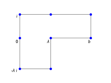
Figure 2: The Weierstrass curve $W_{D}$ emerges from the study of billiards in an $L$-shaped polygon obtained from a $\lambda$-by-$\lambda$ square and a $b$-by-$1$ rectangle where $\lambda=(e+\sqrt{D})/2$, $b=(D-e^{2})/4$ and $e=0$ or $-1$ with $e\equiv D\bmod 2$.

is a Teichmüller curve if $C$ is biholomorphic to a finite volume hyperbolic Riemann surface $\mathbb{H}/\Gamma$ in such a way that $f$ induces a local isometry. The first example of a Teichmüller curve is the modular curve $\mathbb{H}/\operatorname{PSL}_{2}(\mathbb{Z})\to\mathcal{M}_{1}$. Other examples emerge from the study of square-tiled surfaces and billiards in polygons [49]. In genus two, each discriminant $D$ of a real quadratic order determines a Weierstrass curve $W_{D}\to\mathcal{M}_{2}$ (defined below) which is a disjoint union of finitely many Teichmüller curves [30] (see also [8]). The curve $W_{D}$ is related to billiards in the $L$-shaped polygon described in Figure 2 and Weierstrass curves are the main source of Teichmüller curves in $\mathcal{M}_{2}$ [33].

Few explicit algebraic models of Teichmüller curves have appeared in the literature. The current list of examples [6, 7, 24] consists of curves of genus zero and hyperbolic volume at most $3\pi$ and is produced by a variety of ingenious methods which will likely be difficult to extend. In this paper, we describe a general method to determine algebraic models for the Weierstrass curves in genus two. We use our method to describe $W_{D}$ for each of the thirty fundamental discriminants $D<100$. These examples include a Teichmüller curve of genus eight and hyperbolic volume $60\pi$. Our methods are based on the study of certain Hilbert modular forms and a technique for identifying eigenforms for real multiplication on genus two Jacobians based on Ahlfors’s variational formula. We expect that the resulting method to explicitly describe the action of real multiplication on the one-forms of a Riemann surface will be much more broadly applicable. In particular, it should be useful for studying real multiplication in higher genera, and the Prym Teichmüller curves in $\mathcal{M}_{3}$ and $\mathcal{M}_{4}$ [32].

A growing body of literature demonstrates that Teichmüller curves are exceptional from a variety of perspectives. Teichmüller curves have celebrated applications to billiards in polygons and dynamics on translation surfaces [49, 50] and give examples of interesting Fuchsian differential operators [6]. The variations of Hodge structures associated to Teichmüller curves have remarkable properties [37, 36] which suggest that Teichmüller curves are natural relatives of Shimura curves. Each Teichmüller curve, like a Shimura curve, is isometrically immersed in a Hilbert modular variety equipped with its Kobayashi metric and is simultaneously defined as an algebraic curve over a number field and uniformized by a Fuchsian group defined over number field. These facts about Teichmüller curves have been used by several authors to explain the lack of examples in higher genus [3, 28]. A secondary goal of this paper is to present evidence drawn from our examples that Teichmüller curves also admit a rich arithmetic geometry. We show in particular that many of our examples have small and orderly primes of bad reduction and notable divisors supported at their cusps.

Weierstrass curves in Hilbert modular surfaces.

For each integer $D>0$ with $D\equiv 0,1\bmod 4$, let $\mathcal{O}_{D}$ be the quadratic ring of discriminant $D$. The Hilbert modular surface of discriminant $D$ is the complex orbifold $X_{D}=\mathbb{H}\times\mathbb{H}/\operatorname{PSL}(\mathcal{O}_{D}\oplus\mathcal{O}_{D}^{\vee})$. When viewed as an algebraic surface, $X_{D}$ is a moduli space of principally polarized abelian surfaces with real multiplication by $\mathcal{O}_{D}$. The Weierstrass curve of discriminant $D$ is the moduli space $W_{D}$ consisting of pairs $(X,[\omega])$ where: (1) $X$ is a Riemann surface of genus two, (2) $\omega$ is a holomorphic one-form on $X$ with double zero and (3) the Jacobian $\operatorname{Jac}(X)$ admits real multiplication by $\mathcal{O}_{D}$ stabilizing the one-form up to scale $[\omega]$. The period mapping sending a Riemann surface to its Jacobian lifts to an embedding of $W_{D}$ in $X_{D}$.

Explicit algebraic models of Hilbert modular surfaces are obtained in [11] by studying elliptic fibrations of K3 surfaces.

Theorem (Elkies-Kumar).

For fundamental discriminants $1<D<100$, the Hilbert modular surface $X_{D}$ is birational to the degree two cover of the $(r,s)$-plane branched along the curve $b_{D}(r,s)=0$ where $b_{D}$ is the polynomial in Table T.1.

Figure 1: The Hilbert modular surface $X_{44}$ is birational to the degree two cover of the $(r,s)$-plane branched along the curve $b_{44}(r,s)=0$ (dashed). The Weierstrass curve $W_{44}$ is birational to the curve $w_{44}(r,s)=0$ (solid).

The techniques used in [11] also provide an algebraic description of the image of the rational map $X_{D}\to\mathcal{M}_{2}$. However, these techniques do not readily adapt to describe the action of $\mathcal{O}_{D}$ on the Jacobians in $X_{D}$. We address this challenge by developing a method for eigenform location, which computes the action of $\mathcal{O}_{D}$ on the space of holomorphic one-forms on a Riemann surface whose Jacobian lies on $X_{D}$. We use our method, which we describe briefly at the end of this section and more extensively in §4, to identify the locus corresponding to $W_{D}$ in the model for $X_{D}$ above.

Theorem 1.1.

For fundamental discriminants $1<D<100$, the Weierstrass curve $W_{D}$ is birational to the curve $w_{D}(r,s)=0$ where $w_{D}$ is the polynomial in Table T.2.

The first Weierstrass curve of positive genus is the curve $W_{44}$ of genus one. The birational model $w_{44}(r,s)=0$ of $W_{44}$ is depicted in Figure 1 along with the curve $b_{44}(r,s)=0$. Our proof of Theorem 1.1 will yield an explicit birational model of the universal curve over $W_{D}$ for fundamental discriminants $1<D<100$.

Spin components of Weierstrass curves.

The curve $W_{D}$ is irreducible except when $D\equiv 1\bmod 8$ in which case $W_{D}=W_{D}^{0}\sqcup W_{D}^{1}$ is a disjoint union of two irreducible components distinguished by a spin invariant [31]. For such discriminants, the components of $W_{D}$ have Galois conjugate algebraic models defined over $\mathbb{Q}(\sqrt{D})$ [6]. Our next theorem distinguishes the components of reducible $W_{D}$ in the models given in Theorem 1.1.

Theorem 1.2.

For fundamental discriminants $1<D<100$ with $D\equiv 1\bmod 8$, the curve $W_{D}^{\epsilon}$ is birational to the curve $w_{D}^{\epsilon}(r,s)=0$ where $w_{D}^{0}$ is the polynomial in Table T.3 and $w_{D}^{1}$ is the Galois conjugate of $w_{D}^{0}$.

Rational, hyperelliptic and plane quartic models.

The polynomials $w_{D}$ listed in Table T.2 are complicated in part because they reflect how $W_{D}$ is embedded in $X_{D}$. The homeomorphism type of $W_{D}$ is determined in [2, 31, 39] and in Table T.4 we list the homeomorphism type of $W_{D}$ for the discriminants considered in this paper. For fundamental discriminants $D\leq 73$ with $D\neq 69$, the irreducible components of $W_{D}$ have genus at most three and algebraic models simpler than those given by Theorems 1.1 and 1.2.

For discriminants $D\leq 41$, each irreducible component of $W_{D}$ has genus zero. Our proof of Theorems 1.1 and 1.2 will give rational parametrizations of the irreducible components of $w_{D}(r,s)=0$ for such $D$ and yield our next result.

Theorem 1.3.

For fundamental discriminants $D\leq 41$, each component of $W_{D}$ is birational to $\mathbb{P}^{1}$ over $\mathbb{Q}(\sqrt{D})$. For $D\leq 41$ with $D\not\equiv 1\bmod 8$ and $D\neq 21$, the curve $W_{D}$ is also birational to $\mathbb{P}^{1}$ over $\mathbb{Q}$. The curve $W_{21}$ has no rational points and is birational over $\mathbb{Q}$ to the conic $g_{21}(x,y)=0$ where:

$$g_{21}(x,y)=21\left(11x^{2}-182x-229\right)+y^{2}.$$

The curve $W_{44}$ of genus one and the curves $W_{53}$ and $W_{61}$ of genus two are hyperelliptic and the curves $W_{56}$ and $W_{60}$ of genus three are canonically embedded as smooth quartics in $\mathbb{P}^{2}$. Our next theorem identifies hyperelliptic and plane quartic models of these curves.

Theorem 1.4.

For $D\in\left\{44,53,56,60,61\right\}$, the curve $W_{D}$ is birational to $g_{D}(x,y)=0$ where $g_{D}$ is the polynomial listed in Table 1.1.

The irreducible components of $W_{57}$, $W_{65}$ and $W_{73}$ have genus one. We also identify hyperelliptic models of these curves.

Theorem 1.5.

For $D\in\left\{57,65,73\right\}$, the curve $W_{D}^{\epsilon}$ is birational to $g_{D}^{\epsilon}(x,y)=0$ where $g_{D}^{0}$ is the polynomial listed in Table 1.1 and $g_{D}^{1}$ is the Galois conjugate of $g_{D}^{0}$.

Hyperelliptic and plane quartic models of Weierstrass curves
$g_{44}(x,y)=x^{3}+x^{2}+160x+3188-y^{2}$
$g_{53}(x,y)=7711875+3572389x+777989x^{2}+100812x^{3}+8252x^{4}+401x^{5}+9x^{6}-(1+x^{2})y-y^{2}$
$g_{56}(x,y)=35+10x-20x^{2}-2x^{3}+x^{4}-43y+15xy+5x^{2}y-x^{3}y+33y^{2}-xy^{2}-5x^{2}y^{2}-10y^{3}+4xy^{3}+4y^{4}$
$g_{57}^{0}(x,y)=x^{3}+\frac{1}{2}(1+\sqrt{57})x^{2}+(12+\sqrt{57})x+\frac{1}{2}(31-\sqrt{57})-\frac{1}{2}(1+\sqrt{57})xy-y^{2}$
$g_{60}(x,y)=4x^{4}-8x^{3}y-4x^{3}+50x^{2}y^{2}-2x^{2}y-44xy^{3}-56xy^{2}+10xy+228y^{4}-32y^{3}-8y^{2}+y$
$g_{61}(x,y)=12717-527x-6117x^{2}+1498x^{3}-604x^{4}-282x^{5}+324x^{6}-\left(x^{2}+x+1\right)y-y^{2}$
$g_{65}^{0}(x,y)=x^{3}+\left(27\sqrt{65}-229\right)x^{2}+\frac{1}{2}\left(11225\sqrt{65}-90375\right)x-y^{2}$
$g_{73}^{0}(x,y)=x^{3}+\frac{1}{2}(1+\sqrt{73})x^{2}-\frac{1}{2}(701+83\sqrt{73})x-52+36\sqrt{73}-\frac{1}{2}(221+17\sqrt{73})y-y^{2}$

Table 1.1: For discriminants $44\leq D\leq 73$ with $D\neq 69$, each irreducible component of $W_{D}$ has either a hyperelliptic or plane quartic model defined above (cf. Theorems 1.4 and 1.5).

Arithmetic of Teichmüller curves.

We hope that the models of Weierstrass curves in Tables 1.1, T.2 and T.3 will encourage the study of the arithmetic geometry of Teichmüller curves. To that end, we now list several striking facts about these examples that give evidence toward the theme:

Teichmüller curves are arithmetically interesting.

We will denote by $\overline{W}_{D}$ the smooth, projective curve birational to $W_{D}$. The curve $\overline{W}_{D}$ is obtained from $W_{D}$ by filling in finitely many cusps on $W_{D}$ (studied in [31]) and smoothing finitely many orbifold points (studied in [39]). Our rational, hyperelliptic and plane quartic birational models of low genus components of $W_{D}$ extend to biregular models of components of $\overline{W}_{D}$. Throughout what follows, we identify $\overline{W}_{D}$ with these biregular models via the parametrizations given in auxiliary computer files, as described in Section 7.

Singular primes.

The first indication that the curves $\overline{W}_{D}$ have interesting arithmetic is the fact our low, positive genus examples are singular only at small primes. Our next two theorems suggest the following.

The primes of bad reduction for Teichmüller curves
have arithmetic significance.

To formulate a precise statement, we define

$$N(D)=2\cdot D\cdot\prod_{e}\frac{D-e^{2}}{4}\mbox{ where $e$ ranges in }\left\{e:e>0,e\equiv D\bmod 2\mbox{ and }e^{2}<D\right\}.$$ (1.1)

The quantity $N(D)$ bears a striking resemblance to formulas in the arithmetic of “singular moduli” of elliptic curves [12]. The number $N(D)$ is also closely related to the product locus $P_{D}\subset X_{D}$ parametrizing polarized products of elliptic curves with real multiplication. The curve $P_{D}$ is a disjoint union of modular curves each of whose levels divide $N(D)$ ([31], §2). In particular, the primes of bad reduction for $P_{D}$ all divide $N(D)$ [42]. For many of our examples, we find that the same is true of the primes of bad reduction for $\overline{W}_{D}$.

Theorem 1.6.

For discriminants $D\in\left\{21,44,53,56,60,61\right\}$, the curve $\overline{W}_{D}$ has bad reduction at the prime $p$ only if $p$ divides $N(D)$.

For Weierstrass curves birational $\mathbb{P}^{1}$ over $\mathbb{Q}$, we give explicit parametrizations of $\overline{W}_{D}$ by the projective $t$-line in the auxiliary files. We define the cuspidal polynomial $c_{D}(t)$ to be the monic polynomial vanishing simply at the cusps of $\overline{W}_{D}$ in the affine $t$-line and nowhere else, and obtain the following genus zero analogue of Theorem 1.6.

Theorem 1.7.

For $D\leq 41$ with $D\not\equiv 1\bmod 8$ and $D\neq 21$, the cuspidal polynomial $c_{D}(t)$ is in $\mathbb{Z}[t]$ and a prime $p$ divides the discriminant of $c_{D}(t)$ only if $p$ divides $N(D)$.

The primes of singular reduction for our models of low, positive genus Weierstrass curves are listed in Table 7.1 and the cuspidal polynomials for Weierstrass curves birational to $\mathbb{P}^{1}$ over $\mathbb{Q}$ are listed in Table 7.2. Note that it is conceivable that we could get a smaller set of bad primes by choosing a different parametrization.

Divisors supported at cusps.

The divisors supported at cusps of $\overline{W}_{D}$ provide further evidence that Teichmüller curves are arithmetically interesting. The Fuchsian groups presenting Teichmüller curves as hyperbolic orbifolds are examples of Veech groups. Our next three theorems suggest that

Veech groups have a rich theory of modular forms.

Veech groups uniformizing Teichmüller curves can be computed by the algorithm described in [38] and a fundamental domain for the group uniformizing $W_{44}$ is depicted in Figure 3. For background on Veech groups see e.g. [27, 51].

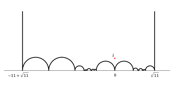
Figure 3: The ideal polygon in $\mathbb{H}$ depicted above is a fundamental domain for the Veech group uniformizing $W_{44}$.

By the Manin-Drinfeld theorem [10, 25], the degree zero divisors supported at the cusps of the modular curve $X_{0}(m)=\overline{\mathbb{H}/\Gamma_{0}(m)}$ generate a finite subgroup of the Picard group $\operatorname{Pic}^{0}(X_{0}(m))$. The same is not quite true for divisors supported at cusps of Weierstrass curves.

Theorem 1.8.

The subgroup of $\operatorname{Pic}^{0}\left(\overline{W}_{44}\right)$ generated by divisors supported at the nine cusps of $W_{44}$ is isomorphic to $\mathbb{Z}^{2}$.

While the cuspidal subgroup of $\overline{W}_{44}$ is not finite, it is small in the sense that there are (many) principal divisors supported at cusps. In other words, there are non-constant regular (algebraic) maps $W_{44}\to\mathbb{C}^{*}$. Several other Weierstrass curves also enjoy this property.

Theorem 1.9.

Each of the curves $W_{44}$, $W_{53}$, $W_{57}$, $W_{60}$, $W_{65}$, and $W_{73}$ admits a non-constant regular (algebraic) map to $\mathbb{C}^{*}$.

For several of the genus two and three Weierstrass curves, we also find canonical divisors supported at cusps.

Theorem 1.10.

Each of the curves $\overline{W}_{53}$, $\overline{W}_{56}$ and $\overline{W}_{60}$ has a holomorphic one-form vanishing only at cusps. The curve $\overline{W}_{61}$ has no holomorphic one-form vanishing only at cusps.

In Figure 4, the plane quartic model for $\overline{W}_{60}$ is shown with the locations of the cusps marked. The five dashed lines meet $\overline{W}_{60}$ only at cusps and each corresponds to a holomorphic one-form up to scale on $\overline{W}_{60}$ vanishing only at cusps. The ratio of two such forms corresponds to a holomorphic map $W_{60}\to\mathbb{C}^{*}$.

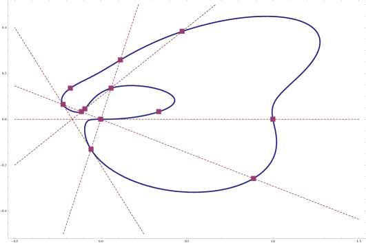
Figure 4: The curve $\overline{W}_{60}$ is biregular to the plane quartic $g_{60}(x,y)=0$ (solid) and the five lines shown (dashed) meet $\overline{W}_{60}$ only at cusps (squares).

Numerical sampling and Hilbert modular forms.

As we now describe, the equations in Table T.2 were obtained by numerically sampling the ratio of certain Hilbert modular forms. For $\tau=(\tau_{1},\tau_{2})\in\mathbb{H}\times\mathbb{H}$, define matrices

$$\Pi(\tau)=\begin{pmatrix}1&\frac{D+\sqrt{D}}{2}&\tau_{1}\frac{1+\sqrt{D}}{2}&\tau_{1}\frac{\sqrt{D}}{D}\\ 1&\frac{D-\sqrt{D}}{2}&\tau_{2}\frac{1-\sqrt{D}}{2}&\tau_{2}\frac{-\sqrt{D}}{D}\end{pmatrix}\mbox{ and }M=\frac{1}{2}\left(\begin{smallmatrix}D+\sqrt{D}&0\\ 0&D-\sqrt{D}\end{smallmatrix}\right).$$ (1.2)

Since multiplication by $M$ preserves the lattice $\Pi(\tau)\cdot\mathbb{Z}^{4}$, the abelian variety $B(\tau)=\mathbb{C}^{2}/\left(\Pi(\tau)\cdot\mathbb{Z}^{4}\right)$ admits real multiplication by $\mathcal{O}_{D}$, and the forms $dz_{1}$ and $dz_{2}$ on $\mathbb{C}^{2}$ cover $\mathcal{O}_{D}$-eigenforms $\eta_{1}(\tau)$ and $\eta_{2}(\tau)$ on $B(\tau)$. There are meromorphic functions $a_{k}:\mathbb{H}\times\mathbb{H}\to\mathbb{C}$ for $0\leq k\leq 5$ so that, for most $\tau\in\mathbb{H}\times\mathbb{H}$, the Jacobian of the algebraic curve

$$Y(\tau)\in\mathcal{M}_{2}\mbox{ birational to the plane curve }z^{2}=w^{6}+a_{5}(\tau)w^{5}+\dots+a_{1}(\tau)w+a_{0}(\tau)$$ (1.3)

is isomorphic to $B(\tau)$ and the forms $\eta_{1}(\tau)$ and $\eta_{2}(\tau)$ pull back under the Abel-Jacobi map $Y(\tau)\to B(\tau)$ to the forms $\omega_{1}(\tau)=dw/z$ and $\omega_{2}(\tau)=w\cdot dw/z$. The functions $a_{k}$ are modular for $\operatorname{PSL}(\mathcal{O}_{D}\oplus\mathcal{O}_{D}^{\vee})$ and the ratio of $a_{0}$ with the Igusa-Clebsch invariant of weight two

$$a_{0}/I_{2}\mbox{ where }I_{2}=-240a_{0}+40a_{1}a_{5}-16a_{2}a_{4}+6a_{3}^{2}$$ (1.4)

is $\operatorname{PSL}(\mathcal{O}_{D}\oplus\mathcal{O}_{D}^{\vee})$-invariant. Since $a_{0}(\tau)$ is zero if and only if $\omega_{2}(\tau)$ has a double zero, $a_{0}/I_{2}$ covers an algebraic function on $X_{D}$ which vanishes along $W_{D}$.

To obtain an explicit model of $W_{D}$, we numerically sample $a_{0}/I_{2}$ using the model of $X_{D}$ in [11] and the Eigenform Location Algorithm we describe below. Alternatively, one can numerically sample $a_{0}/I_{2}$ using the functions in Magma related to analytic Jacobians (cf. [48]). We then interpolate to find an exact rational function $w_{D}(r,s)/I_{2}(r,s)$ which equals $a_{0}/I_{2}$ in these models and whose numerator appears in Table T.2.

The Eigenform Location Algorithm (ELA).

To prove Theorems 1.1 and 1.2, in Section 4 we develop an Eigenform Location Algorithm (ELA, Figure 5). The algorithm takes as input a genus two curve whose Jacobian has real multiplication, and outputs the locations of the eigenforms. Recall that, for $Y\in\mathcal{M}_{2}$, there is a natural pairing between $T_{Y}\mathcal{M}_{2}$ and the space of holomorphic quadratic differentials $Q(Y)$ on $Y$. There is a well-known formula for this pairing which we recall in Section 3 in terms of a hyperelliptic model for $Y$.

Our location algorithm is based on the following theorem, which is a consequence of Ahlfors’s variational formula.

Theorem 1.11.

For $\tau$ in the domain of the meromorphic function $Y:\mathbb{H}\times\mathbb{H}\to\mathcal{M}_{2}$ defined by Equation 1.3, the line in $Q(Y(\tau))$ spanned by the quadratic differential

$$q(\tau)=\omega_{1}(\tau)\cdot\omega_{2}(\tau)$$

annihilates the image of $(dY)_{\tau}$.

Theorem 1.11 characterizes the eigenforms $\omega_{1}(\tau)$ and $\omega_{2}(\tau)$ on $Y(\tau)$ up to permutation and scale. Using an algebraic model for the image of $X_{D}$ in $\mathcal{M}_{2}$ (as in, for example, [11, 13, 41]) and the formula in Section 3, we can use Theorem 1.11 to identify eigenforms for real multiplication. This observation is the basis for ELA. By running ELA with floating point input, we numerically sample the function $a_{0}/I_{2}$ defined in the previous paragraph and generate Tables T.2 and T.3 refered to in Theorems 1.1 and 1.2. By running ELA with input defined over a function field $K$ over a number field (e.g. $K=\mathbb{Q}(r)[s]/(w_{D})$), we prove Theorems 1.1 and 1.2 using only rigorous arithmetic in $K$.

In [21], we will describe a second method of eigenform location based on explicit algebraic correspondences and similar in spirit to [46, 47]. This technique could be used to prove Theorem 1.1 and such a proof would, unlike the proof in this paper, be logically independent of [11]. We found this correspondence method practical for certifying single eigenforms and impractical for certifying positive dimensional families of eigenforms.

Computer files.

Auxiliary files containing extra information on the Weierstrass curves (omitted here for lack of space), as well as computer code to certify our equations, are available from http://arxiv.org/abs/1406.7057. To access these, download the source file for the paper. This will produce both the LaTeX file for this paper and the computer code referenced below. The text file README gives a reader’s guide to the various auxiliary files.

Outline.

We conclude this Introduction by outlining the remaining sections of this paper.

1. We begin in Section 2 by studying families of marked Riemann surfaces whose Jacobians admit real multiplication. We prove that, for a Riemann surface $Y$ whose Jacobian has real multiplication, there is a symplectic basis $U$ for $H_{1}(Y,\mathbb{R})$ consisting of eigenvectors for real multiplication (Proposition 2.2) and that the period matrix for $Y$ with respect to $U$ is diagonal (Proposition 2.3). Using Ahlfors’s variational formula, we deduce Proposition 2.6 which places a condition on eigenform products and generalizes Theorem 1.11.

2. We then study the pairing between the vector spaces $Q(Y)$ and $T_{Y}\mathcal{M}_{2}$ for a genus two Riemann surface $Y$ birational to the plane curve defined by $z^{2}=f(w)$ with $\deg(f)=5$. There is a well known formula for this pairing in terms of the roots of $f(w)$. We recall this formula in Proposition 3.3 and deduce Theorem 3.2 which gives a formula in terms of the coefficients of $f(w)$.

3. In Section 4, we combine the condition on eigenforms imposed by Proposition 2.6 with the pairing given in Section 3 to give an Eigenform Location Algorithm. We demonstrate our algorithm by identifying the eigenforms for real multiplication by $\mathcal{O}_{12}=\mathbb{Z}\left[\sqrt{3}\right]$ on a particular genus two algebraic curve (Theorem 4.1).

4. In Section 5, we implement ELA over function fields to certify our models of irreducible $W_{D}$ and prove Theorems 1.1 and 1.4.

5. We then turn to reducible Weierstrass curves in Section 6. Using the technique in Section 5, we can show that the curve $w_{D}^{0}(r,s)=0$ gives a birational model for an irreducible component of $W_{D}$. In Section 6, we explain how to distinguish between the irreducible components of $W_{D}$ by studying cusps, allowing us to prove Theorems 1.2 and 1.5.

6. In Section 7, we discuss the proofs of the remaining theorems stated in this introduction concerning the arithmetic geometry of Weierstrass curves.

Acknowledgments.

We thank Noam Elkies, Matt Emerton, Curt McMullen, Alex Wright and the anonymous referees for helpful comments. A. Kumar was supported in part by National Science Foundation grant DMS-0952486 and by a grant from the MIT Solomon Buchsbaum Research Fund. R. E. Mukamel was supported in part by National Science Foundation grant DMS-1103654. We used the computer algebra systems gp/Pari [44], Magma [5], Maple [26] and Maxima [29], extensively in our calculations. In particular, most of the auxiliary computer files for verifying our calculations are Magma files (however, they can be easily adapted to different computer algebra systems, such as Sage [43]).

2 Jacobians with real multiplication

Throughout this section, we fix the following:

• a compact topological surface $S$ of genus $g$,

• an order $\mathcal{O}$ in a totally real field $K$ of degree $g$ over $\mathbb{Q}$, and

• a proper, self-adjoint embedding of rings $\rho:\mathcal{O}\rightarrow\operatorname{End}(H_{1}(S,\mathbb{Z}))$.

Here, proper means that $\rho$ does not extend to a larger subring of $K$ and self-adjoint is with respect to the intersection symplectic form $E(S)$ on $H_{1}(S,\mathbb{Z})$, i.e. for each $x,y\in H_{1}(S,\mathbb{Z})$ and $\alpha\in\mathcal{O}$ we have $E(S)(\rho(\alpha)x,y)=E(S)(x,\rho(\alpha)y)$.

Our goal for this section is to define and study the Teichmüller space of the pair $(S,\rho)$. The space $\operatorname{Teich}(S,\rho)$ consists of complex structures $Y$ on $S$ for which $\rho$ extends to real multiplication by $\mathcal{O}$ on $\operatorname{Jac}(Y)$. In Proposition 2.2, we show that there is a basis $U$ for $H_{1}(S,\mathbb{R})$ consisting of eigenvectors for $\rho$. In Proposition 2.3, we show that $Y$ is in $\operatorname{Teich}(S,\rho)$ if and only if the period matrix for $Y$ with respect to $U$ is diagonal. In Proposition 2.6, we combine Ahlfors’s variational formula with Proposition 2.3 to derive a condition satisfied by products of eigenforms for real multiplication on $Y\in\operatorname{Teich}(S,\rho)$. The condition in Theorem 1.11 follows easily from of Proposition 2.6.

The results in the section are, for the most part, well known. We include them as background and to fix notation. In Sections 4 and 5, we will use Proposition 2.6 to certify that certain algebraic one-forms are eigenforms for real multiplication and show that the equations in Table T.2 give algebraic models of Weierstrass curves. For additional background on abelian varieties, Jacobians and their endomorphisms see [4], for background on Hilbert modular varieties see [34, 45] and for background on Teichmüller theory and moduli space of Riemann surfaces see [16, 19, 14].

Teichmüller space of $S$.

Let $\operatorname{Teich}(S)$ be the Teichmüller space of $S$. The space $\operatorname{Teich}(S)$ is the fine moduli space representing the functor sending a complex manifold $B$ to the set of holomorphic families over $B$ whose fibers are marked by $S$ up to equivalence. In particular, a point $Y\in\operatorname{Teich}(S)$ corresponds to an isomorphism class of Riemann surface marked by $S$ and there are canonical isomorphisms $H_{1}(Y,\mathbb{Z})\cong H_{1}(S,\mathbb{Z})$, $\pi_{1}(Y)\cong\pi_{1}(S)$, etc. The space $\operatorname{Teich}(S)$ is a complex manifold homeomorphic to $\mathbb{R}^{6g-6}$ and is isomorphic to a bounded domain in $\mathbb{C}^{3g-3}$.

Moduli space.

Let $\operatorname{Mod}(S)$ denote the mapping class group of $S$, i.e. the group of orientation preserving homeomorphisms from $S$ to itself up to homotopy. The group $\operatorname{Mod}(S)$ acts properly discontinuously on $\operatorname{Teich}(S)$ and the quotient

$$\mathcal{M}_{g}=\operatorname{Teich}(S)/\operatorname{Mod}(S)$$

is a complex orbifold which coarsely solves the moduli problem for unmarked families of Riemann surfaces homeomorphic to $S$. We call $\mathcal{M}_{g}$ the moduli space of genus $g$ Riemann surfaces.

Holomorphic one-forms and Jacobians.

For each $Y\in\mathcal{M}_{g}$, let $\Omega(Y)$ be the vector space of holomorphic one-forms on $Y$ and let $\Omega(Y)^{*}$ be the vector space dual to $\Omega(Y)$. By complex analysis, $\dim_{\mathbb{C}}\Omega(Y)=g$ and the map

$$f:H_{1}(Y,\mathbb{R})\rightarrow\Omega(Y)^{*}\mbox{ given by }f(a)(\omega)=\int_{a}\omega$$ (2.1)

is an $\mathbb{R}$-linear isomorphism. In particular, $f(H_{1}(Y,\mathbb{Z}))$ is a lattice in $\Omega(Y)^{*}$ and the quotient

$$\operatorname{Jac}(Y)=\Omega(Y)^{*}/f(H_{1}(Y,\mathbb{Z}))$$ (2.2)

is a complex torus called the Jacobian of $Y$. The Hermitian form $H^{*}$ on $\Omega(Y)^{*}$ dual to the form

$$H(\omega,\eta)=\frac{i}{2}\int_{Y}\omega\wedge\overline{\eta}\mbox{ for each }\omega,\eta\in\Omega(Y)$$ (2.3)

defines a principal polarization on $\operatorname{Jac}(Y)$ since the pullback of $\operatorname{Im}(H^{*})$ under $f$ restricts to the intersection pairing $E(Y)$ on $H_{1}(Y,\mathbb{Z})$.

Jacobian endomorphisms.

An endomorphism of $\operatorname{Jac}(Y)$ is a holomorphic homomorphism from $\operatorname{Jac}(Y)$ to itself. Since $\operatorname{Jac}(Y)$ is an abelian group, the collection $\operatorname{End}(\operatorname{Jac}(Y))$ of all endomorphisms of $\operatorname{Jac}(Y)$ forms a ring called the endomorphism ring of $\operatorname{Jac}(Y)$. Every endomorphism $R\in\operatorname{End}(\operatorname{Jac}(Y))$ arises from $\mathbb{C}$-linear map $\rho_{a}(R):\Omega(Y)^{*}\to\Omega(Y)^{*}$ preserving the lattice $f(H_{1}(Y,\mathbb{Z}))$. The assignment

$$\rho_{a}:\operatorname{End}(\operatorname{Jac}(Y))\to\operatorname{End}(\Omega(Y)^{*})\mbox{ given by }R\mapsto\rho_{a}(R)$$ (2.4)

is an embedding of rings called the analytic representation of $\operatorname{End}(\operatorname{Jac}(Y))$. We will denote by $\rho_{a}^{*}$ the representation of $\operatorname{End}(\operatorname{Jac}(Y))$ on $\Omega(Y)$ dual to $\rho_{a}$. The assignment

$$\rho_{r}:\operatorname{End}(\operatorname{Jac}(Y))\to\operatorname{End}(H_{1}(Y,\mathbb{Z}))\mbox{ given by }\rho_{r}(R)=f^{-1}\circ\rho_{a}(R)\circ f$$ (2.5)

is also an embedding of rings and is called the rational representation of $\operatorname{End}(\operatorname{Jac}(Y))$.

For any endomorphism $R\in\operatorname{End}(\operatorname{Jac}(Y))$, there is another endomorphism $R^{*}\in\operatorname{End}(\operatorname{Jac}(Y))$ called the adjoint of $R$ and characterized by the property that $\rho_{r}(R^{*})$ is the $E(Y)$-adjoint of $\rho_{r}(R)$. The assignment $R\mapsto R^{*}$ defines an (anti-)involution on $\operatorname{End}(\operatorname{Jac}(Y))$ called the Rosati involution.

Real multiplication.

Recall that $K$ is a totally real number field of degree $g$ over $\mathbb{Q}$ and $\mathcal{O}$ is an order in $K$, i.e. a subring of $K$ which is also a lattice. We will say that $\operatorname{Jac}(Y)$ admits real multiplication by $\mathcal{O}$ if there is

$$\mbox{a proper, self-adjoint embedding }\iota:\mathcal{O}\rightarrow\operatorname{End}(\operatorname{Jac}(Y)).$$ (2.6)

Proper means that $\iota$ does not extend to a larger subring in $K$ and self-adjoint means that $\iota(\alpha)^{*}=\iota(\alpha)$ for each $\alpha\in\mathcal{O}$. If $\mathcal{O}$ is maximal (i.e. $\mathcal{O}$ is not contained in a strictly larger order in $K$) then an embedding $\mathcal{O}\to\operatorname{End}(\operatorname{Jac}(Y))$ is automatically proper.

Teichmüller space of the pair $(S,\rho)$.

Recall that $\rho:\mathcal{O}\to\operatorname{End}(H_{1}(S,\mathbb{Z}))$ is a proper and self-adjoint embedding of rings. For $Y\in\operatorname{Teich}(S)$, we will say that $\rho$ extends to real multiplication by $\mathcal{O}$ on $\operatorname{Jac}(Y)$ if there is

$$\mbox{an embedding }\iota:\mathcal{O}\to\operatorname{End}(\operatorname{Jac}(Y))\mbox{ satisfying }\rho_{r}\circ\iota=\rho.$$ (2.7)

Equivalently, $\rho$ extends to real multiplication if and only if the $\mathbb{R}$-linear extension of $f\circ\rho(\alpha)\circ f^{-1}$ to $\Omega(Y)^{*}$ is $\mathbb{C}$-linear for each $\alpha\in\mathcal{O}$. Since $\rho$ is proper and self-adjoint, an $\iota$ as in Equation 2.7 is automatically proper and self-adjoint in the sense of the previous paragraph. In Equation 2.7, we have implicitly identified $H_{1}(Y,\mathbb{R})$ with $H_{1}(S,\mathbb{R})$ via the marking.

We define the Teichmüller space of the pair $(S,\rho)$ to be the space

$$\operatorname{Teich}(S,\rho)=\left\{Y\in\operatorname{Teich}(S):\mbox{$\rho$ extends to real multiplication by $\mathcal{O}$ on $\operatorname{Jac}(Y)$}\right\}.$$ (2.8)

If $\rho_{1}$ and $\rho_{2}$ are two proper, self-adjoint embeddings $\mathcal{O}\to\operatorname{End}(H_{1}(S,\mathbb{Z}))$ and $g\in\operatorname{Mod}(S)$ is a mapping class such that the induced map on homology $g_{*}\in\operatorname{End}(H_{1}(S,\mathbb{Z}))$ conjugates $\rho_{1}(\alpha)$ to $\rho_{2}(\alpha)$ for each $\alpha\in\mathcal{O}$, then $g$ gives a biholomorphic map between $\operatorname{Teich}(S,\rho_{1})$ and $\operatorname{Teich}(S,\rho_{2})$.

Symplectic $K$-modules and their eigenbases.

The representation

$$\rho_{K}=\rho\otimes_{\mathbb{Z}}\mathbb{Q}:K\rightarrow\operatorname{End}(H_{1}(S,\mathbb{Q}))$$

turns $H_{1}(S,\mathbb{Q})$ into a $K$-module. We begin our study of $\operatorname{Teich}(S,\rho)$ by showing that there is a unique symplectic $K$-module that arises in this way.

Let $E(\operatorname{Tr})$ be the symplectic trace form on $K\oplus K$ defined by

$$E(\operatorname{Tr})\left((x_{1},y_{1}),(x_{2},y_{2})\right)=\operatorname{Tr}^{K}_{\mathbb{Q}}(x_{1}y_{2}-y_{1}x_{2}).$$ (2.9)

It is easy to check that multiplication by $k\in K$ is self-adjoint for $E(\operatorname{Tr})$.

Proposition 2.1.

Regarding $H_{1}(S,\mathbb{Q})$ as a $K$-module via $\rho_{K}=\rho\otimes_{\mathbb{Z}}\mathbb{Q}$, there is a $K$-linear isomorphism

$$T:K\oplus K\rightarrow H_{1}(S,\mathbb{Q})$$

which is symplectic for the trace from $E(\operatorname{Tr})$ on $K\oplus K$ and the intersection form $E(S)$ on $H_{1}(S,\mathbb{Q})$.

Proof.

Choose any $x\in H_{1}(S,\mathbb{Q})$ and set $L=\rho_{K}(K)\cdot x$. Since $\rho_{K}$ is self-adjoint, $L$ is isotropic. The non-degeneracy of the intersection form $E(S)$ ensures that there is a $y\in H_{1}(S,\mathbb{Q})$ such that $E(S)\left(\rho_{K}(k)\cdot x,y\right)=\operatorname{Tr}^{K}_{\mathbb{Q}}(k)$. Define a map $T:K\oplus K\rightarrow H_{1}(S,\mathbb{Q})$ by the formula

$$T(k_{1},k_{2})=\rho_{K}(k_{1})\cdot x+\rho_{K}(k_{2})\cdot y.$$

Clearly, the map $T$ is $K$-linear. An easy computation shows that $T$ satisfies $E(\operatorname{Tr})(v,w)=E(S)(T(v),T(w))$ for each $v,w\in K\oplus K$ which, together with the non-degeneracy of $E(\operatorname{Tr})$, implies that $T$ is a symplectic vector space isomorphism. ∎

Now let $h_{1},\dots,h_{g}:K\rightarrow\mathbb{R}$ be the $g$ places for $K$. Proposition 2.1 allows us to show that there is a symplectic basis for $H_{1}(S,\mathbb{R})$ adapted to $\rho$.

Proposition 2.2.

There is a symplectic basis $U=\left<a_{1},\dots,a_{g},b_{1},\dots,b_{g}\right>$ for $H_{1}(S,\mathbb{R})$ such that

$$\rho(\alpha)a_{i}=h_{i}(\alpha)\cdot a_{i}\mbox{ and }\rho(\alpha)b_{i}=h_{i}(\alpha)\cdot b_{i}\mbox{ for each $\alpha\in\mathcal{O}$.}$$ (2.10)

Proof.

Since the group $H_{1}(S,\mathbb{Q})$ is isomomorphic as a symplectic $K$-module to $K\oplus K$ with the trace pairing $E(\operatorname{Tr})$ (Proposition 2.1), it suffices to construct an analogous basis for $(K\oplus K)\otimes_{\mathbb{Q}}\mathbb{R}$. Let $\alpha_{1},\dots,\alpha_{g}$ be an arbitrary $\mathbb{Q}$-basis for $K$. Since $\operatorname{Tr}:K\times K\to\mathbb{Q}$ is non-degenerate, we can choose $\beta_{1},\dots,\beta_{g}\in K$ so that $\operatorname{Tr}^{K}_{\mathbb{Q}}(\alpha_{i}\beta_{j})=\delta_{ij}$. Setting

$$a_{i}=\sum_{j=1}^{g}(\alpha_{j},0)\otimes h_{i}(\beta_{j})\mbox{ and }b_{i}=\sum_{j=1}^{g}(0,\beta_{j})\otimes h_{i}(\alpha_{j})$$

yields a basis with the desired properties. ∎

The period map.

Now let $\mathcal{H}_{g}$ be the Siegel upper half-space consisting of $g\times g$ symmetric matrices with positive definite imaginary part. The space $\mathcal{H}_{g}$ is equal to an open, bounded and symmetric domain in the $(g^{2}+g)/2$-dimensional space of all symmetric matrices.

As we now describe, the basis $U$ for $H_{1}(S,\mathbb{R})$ given by Proposition 2.2 allows us to define a holomorphic period map from $\operatorname{Teich}(S)$ to $\mathcal{H}_{g}$. For $Y\in\operatorname{Teich}(S)$, we can view $U$ as a basis for $H_{1}(Y,\mathbb{R})$ via the marking by $S$. Let $\left<\omega_{1}(Y),\dots,\omega_{g}(Y)\right>$ be the basis for $\Omega(Y)$ dual to $U$, i.e. such that $\int_{a_{j}}\omega_{k}(Y)=\delta_{jk}$. The period map is defined by

$$P:\operatorname{Teich}(S)\to\mathcal{H}_{g}\mbox{ where }P_{jk}(Y)=\int_{b_{j}}\omega_{k}(Y).$$ (2.11)

Our next proposition characterizes the points in $\operatorname{Teich}(S,\rho)$ [30, §6].

Proposition 2.3.

For $Y\in\operatorname{Teich}(S)$, the homomorphism $\rho$ extends to real multiplication by $\mathcal{O}$ on $\operatorname{Jac}(Y)$ if and only if the period matrix $P(Y)$ is diagonal.

Proof.

From $\int_{a_{j}}\omega_{k}(Y)=\delta_{jk}$ and $P_{jk}(Y)=P_{kj}(Y)=\int_{b_{j}}\omega_{k}(Y)$ we see that the map $f:H_{1}(Y,\mathbb{R})\to\Omega(Y)^{*}$ of Equation 2.1 satisfies $f(b_{j})=\sum_{k=1}^{g}P_{jk}(Y)\cdot f(a_{k})$. In matrix–vector notation, we have

$$(f(b_{1}),f(b_{2}),\dots,f(b_{g}))=P(Y)\cdot(f(a_{1}),f(a_{2}),\dots,f(a_{g})).$$ (2.12)

For $\alpha\in\mathcal{O}$, let $h(\alpha)$ be the $g\times g$ diagonal matrix with diagonal entries $(h_{1}(\alpha),\dots,h_{g}(\alpha))$. From Equation 2.10, the map $T(\alpha)=f\circ\rho(\alpha)\circ f^{-1}$ extends $\mathbb{C}$-linearly to $\Omega(Y)^{*}$ if and only if the matrix for $T(\alpha)$ is $h(\alpha)$ with respect to both the basis $\left<f(a_{1}),\dots,f(a_{g})\right>$ and the basis $\left<f(b_{1}),\dots,f(b_{g})\right>$. From Equation 2.12 this happens if and only if $P(Y)$ commutes with $h(\alpha)$. Since the embeddings $h_{1},\dots,h_{g}:\mathcal{O}\to\mathbb{R}$ are pairwise distinct, $P(Y)$ commutes with $h(\alpha)$ for every $\alpha\in\mathcal{O}$ if and only if $P(Y)$ is diagonal. ∎

Eigenforms for real multiplication.

For $Y\in\operatorname{Teich}(S,\rho)$ and $\iota$ satisfying $\rho_{r}\circ\iota=\rho$, we saw in the proof of Proposition 2.3 that the matrix for $\rho_{a}(\iota(\alpha))$ with respect to the basis $\left<f(a_{1}),\dots,f(a_{g})\right>$ for $\Omega(Y)^{*}$ is the diagonal matrix $h(\alpha)$. Since this basis is dual to the basis $\left<\omega_{1}(Y),\dots,\omega_{g}(Y)\right>$ for $\Omega(Y)$, we see that $\rho_{a}^{*}(\iota(\alpha))\in\operatorname{End}(\Omega(Y))$ stabilizes $\omega_{i}(Y)$ up to scale. We record this fact in the following proposition.

Proposition 2.4.

For $Y\in\operatorname{Teich}(S,\rho)$ and $\alpha\in\mathcal{O}$, we have that $\rho_{a}^{*}(\alpha)\omega_{i}(Y)=h_{i}(\alpha)\omega_{i}(Y)$.

In light of Proposition 2.4, we call the non-zero scalar multiples of $\omega_{i}(Y)$ the $h_{i}$-eigenforms for $\mathcal{O}$.

Moduli of abelian varieties.

Now consider the homomorphism $M:\operatorname{PSp}(H_{1}(S,\mathbb{R}))\to\operatorname{PSp}_{2g}(\mathbb{R})$ sending a projective symplectic automorphism of $H_{1}(S,\mathbb{R})$ to its matrix with respect to $U$. There is an action of $\operatorname{PSp}_{2g}(\mathbb{R})$ on $\mathcal{H}_{g}$ by holomorphic automorphisms via generalized Möbius transformations such that, for $h\in\operatorname{Mod}(S)$ inducing $h_{*}\in\operatorname{End}(H_{1}(S,\mathbb{Z}))$, we have

$$M(h_{*})\cdot P(Y)=P(h\cdot Y).$$ (2.13)

We conclude that the period map $P:\operatorname{Teich}(S)\to\mathcal{H}_{g}$ covers a holomorphic map

$$\operatorname{Jac}:\mathcal{M}_{g}\to A_{g}=\mathcal{H}_{g}/\Gamma_{\mathbb{Z}}\mbox{ where }\Gamma_{\mathbb{Z}}=M(\operatorname{PSp}(H_{1}(S,\mathbb{Z}))).$$ (2.14)

We also call this map the period map and denote it by $\operatorname{Jac}$ since the space $A_{g}$ has a natural interpretation as a moduli space of principally polarized abelian varieties so that $\operatorname{Jac}$ is simply the map sending a Riemann surface to its Jacobian.

Hilbert modular varieties.

Let $\Delta_{g}$ denote the collection of diagonal matrices in $\mathcal{H}_{g}$ and let $\operatorname{PSp}(H_{1}(S,\mathbb{Z}),\rho)$ denote the subgroup of $\operatorname{PSp}(H_{1}(S,\mathbb{Z}))$ represented by symplectic automorphisms commuting with $\rho(\alpha)$ for each $\alpha\in\mathcal{O}$. The group $\Gamma_{\rho}=M(\operatorname{PSp}(H_{1}(S,\mathbb{Z}),\rho))$ consists of matrices whose $g\times g$ blocks are diagonal. Consequently, $\Gamma_{\rho}$ preserves $\Delta_{g}$ and, by Proposition 2.3, the map $\operatorname{Teich}(S,\rho)\to A_{g}$ covered by the period map $P$ factors through the orbifold

$$X_{\rho}=\Delta_{g}/\Gamma_{\rho}.$$ (2.15)

The space $X_{\rho}$ has a natural interpretation as a moduli space of abelian varieties with real multiplication. Each of the complex orbifolds $\mathcal{M}_{g}$, $A_{g}$ and $X_{\rho}$ can be given the structure of an algebraic variety so that the map in the period map $\operatorname{Jac}$ and the map $X_{\rho}\to A_{g}$ covered by the inclusion $\Delta_{g}\to\mathcal{H}_{g}$ are algebraic. The variety $X_{\rho}$ is called a Hilbert modular variety.

Tangent and cotangent space to $\operatorname{Teich}(S)$.

For $Y\in\operatorname{Teich}(S)$, let $B(Y)$ denote the vector space of $L^{\infty}$-Beltrami differentials on $Y$. The measurable Riemann mapping theorem can be used to give a marked family over the unit ball $B^{1}(Y)$ in $B(Y)$ and construct a holomorphic surjection $\phi:B^{1}(Y)\to\operatorname{Teich}(S)$ with $\phi(0)=Y$. There is a pairing between $B(Y)$ and the space of holomorphic quadratic differentials $Q(Y)$ on $Y$ given by

$$B(Y)\times Q(Y)\to\mathbb{C}\mbox{ where }(\mu,q)\mapsto\int_{Y}\mu\cdot q.$$ (2.16)

Now let $Q(Y)^{\perp}\subset B(Y)$ be the vector subspace consisting of Beltrami differentials annihilating every quadratic differential under the pairing in Equation 2.16. By Teichmüller theory, the space $Q(Y)^{\perp}$ is closed, has finite codimension and is equal to the kernel of $d\phi_{0}$. The tangent space $T_{Y}\operatorname{Teich}(S)$ is isomorphic to $B(Y)/Q(Y)^{\perp}$ and the pairing in Equation 2.16 covers a pairing between $T_{Y}\operatorname{Teich}(S)$ and $Q(Y)$ giving an isomorphism

$$T_{Y}^{*}\operatorname{Teich}(S)\cong Q(Y).$$ (2.17)

The pairing in Equation 2.16 and the isomorphism in Equation 2.17 are $\operatorname{Mod}(S)$-equivariant, and they give rise to a pairing between $Q(Y)$ and the orbifold tangent space $T_{Y}\mathcal{M}_{g}$.

Ahlfors’s variational formula and eigenform products.

Ahlfors’s variational formula expresses the derivative of the period map in terms of quadratic differentials.

Theorem 2.5 (Ahlfors, [1]).

For any $Y\in\operatorname{Teich}(S)$, the derivative of the $(j,k)^{\text{\tiny{th}}}$ coefficient of the period map is the quadratic differential

$$d\left(P_{jk}\right)_{Y}=\omega_{j}(Y)\cdot\omega_{k}(Y).$$ (2.18)

Combining Equation 2.18 with our characterization of the period matrices of $Y\in\operatorname{Teich}(S,\rho)$ yields the following proposition, implicit in [30, proof of Theorem 7.5].

Proposition 2.6.

Suppose $B$ is a smooth manifold and $g:B\rightarrow\operatorname{Teich}(S,\rho)$ is a smooth map. For each $j\neq k$ and $b\in B$, the quadratic differential

$$q_{jk}(b)=\omega_{j}(g(b))\cdot\omega_{k}(g(b))\in Q(g(b))$$

annihilates the image of $dg_{b}$ in $T_{g(b)}\operatorname{Teich}(S)$.

Proof.

In light of Proposition 2.3, the image of $P\circ g$ is contained within the set $\Delta_{g}$ of diagonal matrices in $\mathcal{H}_{g}$. For $j\neq k$, the composition $P_{jk}\circ g:B\rightarrow\mathbb{C}$ is identically zero. The differential $dP_{jk}$ annihilates the image of $dg_{b}$ by the chain rule and is equal to $q_{jk}(b)$ by Ahlfors’s variational formula. ∎

Theorem 1.11 is a special case of Proposition 2.6.

Proof of Theorem 1.11.

Fix $\tau$ in the domain for the map $Y:\mathbb{H}\times\mathbb{H}\to\mathcal{M}_{2}$ defined in Equation 1.3 and let $B$ be a neighborhood of $\tau$ on which $Y$ lifts to a map $\widetilde{Y}:B\to\operatorname{Teich}(S)$ for a genus two surface $S$. Identify $H_{1}(S,\mathbb{Z})$ with $H_{1}(\widetilde{Y}(\tau),\mathbb{Z})$ via the marking and with the lattice $\Pi(\tau)\cdot\mathbb{Z}^{4}=H_{1}(B(\tau),\mathbb{Z})$ (Equation 1.2) via the Abel-Jacobi map $\widetilde{Y}(\tau)\to B(\tau)$ and let $\rho:\mathcal{O}_{D}\to\operatorname{End}(H_{1}(S,\mathbb{Z}))$ be the proper, self-adjoint embedding with $\rho(\alpha)$ equal to multiplication by the diagonal matrix $\operatorname{Diag}\left(h_{1}(\alpha),h_{2}(\alpha)\right)$ on $\Pi(\tau)\cdot\mathbb{Z}^{4}$. Clearly, the lift $\widetilde{Y}$ maps $B$ into $\operatorname{Teich}(S,\rho)$ and Proposition 2.6 shows that the product $\omega_{1}(\tau)\cdot\omega_{2}(\tau)$ annihilates the image of $d\widetilde{Y}_{\tau}$. ∎

Genus two Jacobians with real multiplication.

For typical pairs $(S,\rho)$, we know little else about the space $\operatorname{Teich}(S,\rho)$ including whether or not $\operatorname{Teich}(S,\rho)$ is empty. For the remainder of this section, we impose the additional assumption that $g=2$ so that we can say more.

Let $D$ be the discriminant of $\mathcal{O}$. The first special feature when $g=2$ is that the order $\mathcal{O}$ is determined by $D$ and is isomorphic to $\mathcal{O}_{D}=\mathbb{Z}\left[\frac{D+\sqrt{D}}{2}\right]$. The discriminants of real quadratic orders are precisely the integers $D>0$ and congruent to $0$ or $1\bmod 4$, and the order of discriminant $D$ is an order in a real quadratic field if and only if $D$ is not a square. The discriminant $D$ is fundamental and the order $\mathcal{O}_{D}$ is maximal if $\mathcal{O}_{D}$ is not contained in a larger order in $\mathcal{O}_{D}\otimes\mathbb{Q}$.

The second special feature when $g=2$ is that, for each real quadratic order $\mathcal{O}$, there is a unique proper, self-adjoint embedding $\rho:\mathcal{O}\to H_{1}(S,\mathbb{Z})$ up to conjugation by elements of $\operatorname{Sp}(H_{1}(S,\mathbb{Z}))$ ([41], Theorem 2). Since $\operatorname{Mod}(S)\to\operatorname{Sp}(H_{1}(S,\mathbb{Z}))$ is onto, the spaces $\operatorname{Teich}(S,\rho)$ and $X_{\rho}$ and the maps to $\operatorname{Teich}(S,\rho)\to\mathcal{M}_{2}$ and $X_{\rho}\to A_{2}$ are determined by $D$ up to isomorphism. The Hilbert modular variety $X_{\rho}$ is isomorphic to the Hilbert modular surface of discriminant $D$

$$\begin{array}[]{c}X_{D}=\mathbb{H}\times\mathbb{H}/\operatorname{PSL}(\mathcal{O}_{D}\oplus\mathcal{O}_{D}^{\vee})\mbox{ where }\mathcal{O}_{D}^{\vee}=\frac{1}{\sqrt{D}}\cdot\mathcal{O}_{D}\mbox{ and}\\ \operatorname{PSL}(\mathcal{O}_{D}\oplus\mathcal{O}_{D}^{\vee})=\left\{\begin{pmatrix}a&b\\ c&d\end{pmatrix}\in\operatorname{PSL}_{2}(K):\begin{array}[]{c}ad-bc=1,a,d\in\mathcal{O}_{D}\\ b\cdot\mathcal{O}_{D}^{\vee}\subset\mathcal{O}_{D}\mbox{ and }c\cdot\mathcal{O}_{D}\subset\mathcal{O}_{D}^{\vee}\end{array}\right\}.\end{array}$$ (2.19)

The two places $h_{1},h_{2}:\mathcal{O}_{D}\to\mathbb{R}$ give two homomorphisms $\operatorname{PSL}(\mathcal{O}_{D}\oplus\mathcal{O}_{D}^{\vee})\to\operatorname{PSL}_{2}(\mathbb{R})$ which we also denote by $h_{1}$ and $h_{2}$. The action of $M\in\operatorname{PSL}(\mathcal{O}_{D}\oplus\mathcal{O}_{D}^{\vee})$ on $\mathbb{H}\times\mathbb{H}$ is the ordinary action of $h_{1}(M)$ by Möbius transformation the first coordinate and by $h_{2}(M)$ on the second.

The third special feature when $g=2$ is that the algebraic map $\operatorname{Jac}:\mathcal{M}_{2}\to A_{2}$ is birational with rational inverse $\operatorname{Jac}^{-1}$. Composing $\operatorname{Jac}^{-1}$ with the natural map $X_{D}\to A_{2}$ gives a rational inverse period map

$$\operatorname{Jac}_{D}^{-1}:X_{D}\to\mathcal{M}_{2}$$ (2.20)

whose image is covered by $\operatorname{Teich}(S,\rho)$.

3 Quadratic differentials and residues

To make use of Proposition 2.6 for a complex structure $Y\in\operatorname{Teich}(S,\rho)$ represented by an algebraic curve, we will need an algebraic formula for the pairing between $Q(Y)$ and $T_{Y}\operatorname{Teich}(S)$ described in Equation 2.17. When the genus of $S$ is two, the curve $Y$ is biholomorphic to a hyperelliptic curve defined by an equation of the form $z^{2}=f_{a}(w)$ where

$$f_{a}(w)=w^{5}+a_{4}w^{4}+a_{3}w^{3}+a_{2}w^{2}+a_{1}w+a_{0}$$ (3.1)

for some $a=(a_{0},\dots,a_{4})\in\mathbb{C}^{5}$. There is a well known formula for the pairing between $Q(Y)$ and $T_{Y}\operatorname{Teich}(S)$ for such curves involving residues and the roots of $f_{a}(w)$. We recall this formula in Proposition 3.3. From Proposition 3.3, we deduce Theorem 3.2 which gives a formula in terms of the coefficients of $f_{a}(w)$. Theorem 3.2 is useful from a computational standpoint since the field $\mathbb{Q}(a_{0},\dots,a_{4})$ is typically simpler than the splitting field of $f_{a}(w)$ over $\mathbb{Q}$.

Pairing and polynomial coefficients.

For any $a=(a_{0},\dots,a_{4})\in\mathbb{C}^{5}$, let $f_{a}(w)$ be the polynomial defined in Equation 3.1 and set

$$V=\left\{a\in\mathbb{C}^{5}:\operatorname{Disc}(f_{a}(w))\neq 0\right\}.$$ (3.2)

Consider the holomorphic and algebraic map

$$Y:V\to\mathcal{M}_{2}\mbox{ where $Y(a)$ is birational to the curve defined by $z^{2}=f_{a}(w)$.}$$

While the universal curve over $\mathcal{M}_{2}$ is not a fiber bundle, its pullback to $V$ is a fiber bundle. By Teichmüller theory, the map $Y$ lifts locally to $\operatorname{Teich}(S)$ and, for any $a\in V$, the derivative $(dY)_{a}$ gives rise to a pairing

$$Q(Y(a))\times T_{a}V\to\mathbb{C}.$$ (3.3)

The tangent space $T_{a}V$ is naturally isomorphic to $\mathbb{C}^{5}$ since $V$ is open in $\mathbb{C}^{5}$ and we can identify the vector space $Q(Y(a))$ with $\mathbb{C}^{3}$ by associating $x=(x_{0},x_{1},x_{2})$ with the quadratic differential

$$q_{x}=Q_{x}(w)\cdot\frac{dw^{2}}{f_{a}(w)}\mbox{ where $Q_{x}(w)=x_{0}+x_{1}w+x_{2}w^{2}$}.$$ (3.4)

Our main goal for this section is to establish a formula for the pairing in Equation 3.3 in these coordinates. We start with the following proposition.

Proposition 3.1.

For any integer $k\geq 2$, the function

$$M_{k}(a)=\sum_{\begin{subarray}{c}r\in Z(f_{a})\end{subarray}}\frac{r^{k}}{\left(rf_{a}^{\prime}(r)\right)^{2}}\mbox{ where }Z(f_{a})=\left\{r\in\mathbb{C}:f_{a}(r)=0\right\}$$ (3.5)

is a rational function in $\mathbb{C}\left(a_{0},\dots,a_{4}\right)$ and the product $\operatorname{Disc}\left(f_{a}(w)\right)\cdot M_{k}(a)$ is in $\mathbb{C}[a_{0},\dots,a_{4}]$.

Proof.

The function $M_{k}(a)$ is a rational function in $\mathbb{C}\left(a_{0},\dots,a_{4}\right)$ since the sum in Equation 3.5 is a symmetric rational function of the roots of $f_{a}(w)$. That $\operatorname{Disc}\left(f_{a}(w)\right)\cdot M_{k}(a)$ is a polynomial for $k\geq 2$ follows from the fact that $\operatorname{Disc}(f_{a}(w))/f_{a}^{\prime}(r)^{2}=\operatorname{Disc}\left(f_{a}(w)/(w-r)\right)$ for each $r\in Z(f_{a})$. ∎

We can now state our main theorem for this section.

Theorem 3.2.

For any $a\in V$, $v\in T_{a}V$ and $x\in\mathbb{C}^{3}$, the pairing between the quadratic differential $q_{x}\in Q(Y(a))$ and $v$ is given by

$$q_{x}(v)=(2\pi)\cdot x^{T}\cdot M(a)\cdot v$$ (3.6)

where $M(a)$ is the $3\times 5$-matrix with entries in $\operatorname{Disc}(f_{a}(w))^{-1}\cdot\mathbb{C}\left[a_{0},\dots,a_{4}\right]$ whose $(j,k)^{\text{\tiny{th}}}$ coefficient is the rational function $(M(a))_{jk}=M_{j+k}(a)$ defined in Equation 3.5.

Many computer algebra systems will readily compute an explicit formula for $M_{k}(a)$ for any particular $k$ and in the auxiliary files we include an explicit formula for $M(a)$ (which involves the polynomials $M_{k}(a)$ for $2\leq k\leq 8$). We will prove Theorem 3.2 at the end of this section.

Pairing and roots of polynomials.

For any $r=(r_{1},\dots,r_{5})\in\mathbb{C}^{5}$, let $a(r)=(a_{0}(r),\dots,a_{4}(r))$ be the coefficients of the monic, degree five polynomials with roots $r_{i}$ and define

$$V^{rts}=\left\{r\in\mathbb{C}^{5}:a(r)\in V\right\}.$$

The universal curve over $\mathcal{M}_{2}$ pulls back under $Y\circ a:V^{rts}\to\mathcal{M}_{2}$ to a fiber bundle. As in the previous paragraph, Teichmüller theory gives rise to a natural pairing between $T_{r}V^{rts}$ and $Q(Y(a(r)))$ for any $r\in V^{rts}$. The tangent space $T_{r}V^{rts}$ is naturally isomorphic to $\mathbb{C}^{5}$ since $V^{rts}$ is open in $\mathbb{C}^{5}$ and we can identify $Q(Y(a(r)))$ with $\mathbb{C}^{3}$ via Equation 3.4.

Let $N(r)$ be the $3\times 5$-matrix whose $(j,k)$-th coefficient is the rational function

$$N(r)_{jk}=-\operatorname{Res}_{r_{j}}\left(\frac{w^{k-1}}{f_{a(r)}(w)}\right)=-r_{j}^{k-1}\cdot\prod_{m\neq j}\frac{1}{r_{m}-r_{j}}\mbox{ for $1\leq j\leq 5$ and $1\leq k\leq 3$.}$$ (3.7)

Our next proposition expresses the pairing $Q(Y(a(r)))\times T_{r}V^{rts}\to\mathbb{C}$ in terms of $N(r)$.

Proposition 3.3.

For any $r\in V$, $u\in T_{r}V^{rts}$ and $x\in\mathbb{C}^{3}$, the pairing between the quadaratic differential $q_{x}\in Q(Y(a(r)))$ and $u$ is given by

$$q_{x}(u)=(2\pi)\cdot x^{T}\cdot N(r)\cdot u.$$ (3.8)

Proposition 3.3 is well-known. We include a proof for completeness.

Proof.

Recall that the Riemann surface $Y(a)$ is birational to the algebraic curve $z^{2}=f_{a}(w)$. Let $r=(r_{1},\dots,r_{5})$ and $u=(u_{1},\dots,u_{5})$. One can construct a smoothly varying family of diffeomorphisms

$$\Phi_{t}(w,z)=(W_{t}(w,z),Z_{t}(w,z)):Y\left(a(r)\right)\rightarrow Y\left(a(r+tu)\right)\mbox{ for $t$ small}$$

such that $W_{t}(w,z)=w+tu_{i}$ for $w$ in a neighborhood of $w^{-1}(r_{j})$, $W_{t}(w,z)=w$ for $w$ in a neighborhood of $\infty$ and $\Phi_{0}=\operatorname{id}|_{Y(a(r))}$. Since $\Phi_{t}$ is holomorphic for large $w$, the Beltrami differential $\mu(\Phi_{t})$ is supported away from $w^{-1}(\infty)$ and our computation below is unaffected by our identification of $Y(a(r+tu))$ with the affine plane curve $z^{2}=f_{a(r+tu)}(w)$.

The family of Beltrami differentials $\mu\left(\Phi_{t}\right)=\overline{\partial}\Phi_{t}/\partial\Phi_{t}$ provides a lift of the local map from $V^{rts}$ into $\operatorname{Teich}(S)$ to a map into the unit ball $B^{1}(Y(a(r)))$ in the space of $L^{\infty}$-Beltrami differentials on $Y(a(r))$. To compute $q_{x}(u)$, we compute $\mu\left(\Phi_{t}\right)$ to first order in $t$ and evaluate the right hand side of

$$q_{x}(u)=\lim_{t\rightarrow 0}\frac{1}{t}\int_{Y\left(a(r)\right)}\mu(\Phi_{t})q_{x}.$$ (3.9)

Compare Equation 3.9 with Equation 2.16. Since $\Phi_{t}$ is holomorphic in a neighborhood of the zeros and poles of the meromorphic one-form $dw$ on $Y\left(a(r)\right)$, the Beltrami differential $\mu\left(\Phi_{t}\right)$ satisfies

$$\mu\left(\Phi_{t}\right)=\frac{\overline{\partial}\Phi_{t}}{\partial\Phi_{t}}=\frac{\partial W_{t}(w,z)/\partial\overline{w}\cdot d\overline{w}}{\partial W_{t}(w,z)/\partial w\cdot dw}=\frac{\partial W_{t}(w,z)/\partial\overline{w}}{1+O(t)}\cdot\frac{d\overline{w}}{dw}=\partial W_{t}(w,z)/\partial\overline{w}\cdot\frac{d\overline{w}}{dw}+O(t^{2}).$$ (3.10)

The product $q_{x}\cdot\mu\left(\Phi_{t}\right)$ is supported away from small disks about the Weierstrass points of $Y\left(a(r)\right)$. From Equation 3.10 we see that the product $q_{x}\cdot\mu\left(\Phi_{t}\right)$ is nearly exact in such a neighborhood, i.e.

$$q_{x}\cdot\mu\left(\Phi_{t}\right)=\frac{Q_{x}(w)\partial W_{t}/\partial\overline{w}}{f_{a(r)}(w)}|dw|^{2}+O(t^{2})=d\eta+O(t^{2})\mbox{ where }\eta=\frac{i}{2}\cdot\frac{(W_{t}(w,z)-w)\cdot Q_{x}(w)}{f_{a(r)}(w)}dw.$$ (3.11)

The factor of $i/2$ arises from the equation $|dw|^{2}=(i/2)\cdot dw\wedge d\overline{w}$. Stokes’ theorem gives

$$\int_{Y(a(r))}q_{x}\cdot\mu\left(\Phi_{t}\right)=\int_{C_{\infty}}\eta+\sum_{j=1}^{5}\int_{C_{j}}\eta+O(t^{2})$$ (3.12)

where $C_{j}$ is a small loop around $w^{-1}(r_{j})$ and $C_{\infty}$ is a small loop around $w^{-1}(\infty)$. Since the one-form $\eta$ equals $(i/2)\cdot tu_{j}Q_{x}(w)dw/f_{a(r)}(w)$ in a neighborhood of $w^{-1}(r_{j})$ and is identically zero in a neighborhood of $w^{-1}(\infty)$, we conclude that

$$q_{x}(u)=(-2\pi)\cdot\sum_{j=1}^{5}u_{j}\operatorname{Res}_{r_{j}}\left(\frac{Q_{x}(w)}{f_{a(r)}(w)}dw\right)=(2\pi)\cdot x^{T}\cdot N(r)\cdot u.$$

Note the extra factor of two arising from the fact that $w$ maps $C_{j}\subset Y\left(a(r)\right)$ to a closed curve on the $w$-sphere winding twice about $r_{j}$. ∎

We are now ready to prove Theorem 3.2.

Proof of Theorem 3.2.

For any $r\in V^{rts}$, set $Q(r)=Q(Y(a(r)))$. The pairings $Q(r)\times T_{a(r)}V\to\mathbb{C}$ and $Q(r)\times T_{r}V^{rts}\to\mathbb{C}$ correspond to linear maps $L_{r}:T_{r}V^{rts}\to(Q(r))^{*}$ and $L_{a}:T_{a(r)}V\to(Q(r))^{*}$ which are related to one another by composition with the derivative of $a:V^{rts}\to V$, i.e. $L_{r}=L_{a}\circ da_{r}$. By Proposition 3.3, the matrix $N(r)$ is the matrix for $L_{r}$ with respect to the bases for $Q(r)$ and $T_{r}V^{rts}$ discussed above.

One can give a conceptual proof that the derivative $da_{r}$, the matrix $N(r)$ defined by Equation 3.7 and the matrix $M(a)$ whose $(j,k)$-th coefficient is the polynomial $M_{j+k}(a)$ defined in Equation 3.5 are related by

$$N(r)=\frac{M(a(r))\cdot da_{r}}{\operatorname{Disc}(f_{a(r)}(w))}.$$ (3.13)

We include a program to verify Equation 3.13 in the auxiliary computer files. We conclude $q_{x}(v)$ and $M(a)$ satisfy Equation 3.6. ∎

4 The eigenform location algorithm

In this section, we develop a method of eigenform location based on the condition on eigenform products imposed by Proposition 2.6 and the formula in Theorem 3.2. We demonstrate our method by proving the following theorem.

Theorem 4.1.

The Jacobian of the algebraic curve $Y$ with Weierstrass model

$$z^{2}=w^{5}-2w^{4}-12w^{3}-8w^{2}+52w+24$$ (4.1)

admits real multiplication by $\mathcal{O}_{12}=\mathbb{Z}\left[\sqrt{3}\right]$ with eigenforms $dw/z$ and $w\cdot dw/z$.

Since the one-form $dw/z$ has a double zero, Theorem 4.1 immediately implies the following.

Corollary 4.2.

The one-form up to scale $(Y,[dw/z])$ defined by Equation 4.1 lies on $W_{12}$.

We conclude this section by summarizing our method in the Eigenform Location Algorithm (ELA, Figure 5). Our proof of Theorem 4.1 is to implement ELA with input defined over $\mathbb{Q}$. We can implement ELA with floating point input to numerically sample the function in Equation 1.4 and generate the polynomials in Table T.2 giving algebraic models of Weierstrass curves. In subsequent sections, we will implement ELA with input defined over function fields over number fields to certify our algebraic models of Weierstrass curves and prove Theorems 1.1 and 1.2.

Igusa-Clebsch invariants.

For a genus two topological surface $S$, the Igusa-Clebsch invariants define a holomorphic map $IC:\operatorname{Teich}(S)\rightarrow\mathbb{P}(2,4,6,10)$ where $\mathbb{P}(2,4,6,10)$ is the weighted projective space

$$\mathbb{P}(2,4,6,10)=\mathbb{C}^{4}/\mathbb{C}^{*}\mbox{ where $\mathbb{C}^{*}$ acts by }\lambda\cdot(I_{2},I_{4},I_{6},I_{10})=(\lambda^{2}I_{2},\lambda^{4}I_{4},\lambda^{6}I_{6},\lambda^{10}I_{10}).$$ (4.2)

The coordinate $I_{k}$ of $IC$ is called the Igusa-Clebsch invariant of weight $k$ (cf. [18]).

For $a\in V$ and $Y(a)\in\mathcal{M}_{2}$ as defined in Section 3, the invariants $I_{k}(Y(a))$ are polynomial in $a$. The invariant $I_{10}$ is the discriminant of the polynomial $f_{a}(w)$ and the curve $Y$ defined by Equation 4.1 has

$$IC(Y)=(56:-32:-348:-324).$$

Just as the $j$-invariant gives an algebraic bijection between $\mathcal{M}_{1}$ and $\mathbb{C}$, the Igusa-Clebsch invariants give an algebraic bijection between $\mathcal{M}_{2}$ and $\mathbb{C}^{3}$. The map $IC:\operatorname{Teich}(S)\rightarrow\mathbb{P}(2,4,6,10)$ is $\operatorname{Mod}(S)$ invariant and covers a bijection between $\mathcal{M}_{2}$ and the hyperplane complement

$$\left\{(I_{2}:I_{4}:I_{6}:I_{10}):I_{10}\neq 0\right\}\subset\mathbb{P}(2,4,6,10).$$ (4.3)

Real multiplication by $\mathcal{O}_{12}$.

Recall from Section 2 that the Hilbert modular surface

$$X_{12}=\mathbb{H}\times\mathbb{H}/\operatorname{PSL}(\mathcal{O}_{12}\oplus\mathcal{O}_{12}^{\vee})$$

admits an inverse period map $\operatorname{Jac}_{12}^{-1}:X_{12}\to\mathcal{M}_{2}$ which is a rational map parametrizing the collection of genus two surfaces whose Jacobians admit real multiplication by $\mathcal{O}_{12}$ (cf. Equation 2.20). Set $H_{12}=\mathbb{C}^{2}$ (the $(r,s)$-plane) and consider the map $IC_{12}:H_{12}\rightarrow\mathbb{P}(2,4,6,10)$ defined by

$$IC_{12}(r,s)=\big{(}-8(3+3r-3s-2s^{2}+2s^{3}):4(s-1)^{2}(9r+15rs+s^{4}):\\ -4(s-1)^{2}(72r+90r^{2}+48rs+102r^{2}s-141rs^{2}-38rs^{3}+8s^{4}+67rs^{4}-8s^{5}-6s^{6}+6s^{7})\\ :-4r^{3}(s-1)^{6}\big{)}.$$ (4.4)

The map above is defined in [11], where it is shown that the map $X_{12}\to\mathbb{P}(2,4,6,10)$ factors through $IC_{12}$.

Theorem 4.3 (Elkies-Kumar).

The rational map $IC\circ\operatorname{Jac}_{12}^{-1}:X_{12}\to\mathbb{P}(2,4,6,10)$ is the composition of a degree two rational map $X_{12}\rightarrow H_{12}$ branched along the curve

$$b_{12}(r,s)=0\mbox{ where }b_{12}(r,s)=(s-1)(s+1)(16r+27r^{2}-18rs^{2}-s^{4}+s^{6})$$ (4.5)

and the map $IC_{12}:H_{12}\to\mathbb{P}(2,4,6,10)$.

Compare Equation 4.5 with Table T.1. From Theorem 4.3 we see that $\operatorname{Jac}(Y)$ admits real multiplication by $\mathcal{O}_{12}$ if and only if $IC(Y)$ is in the closure of the image of $IC_{12}$.

Proposition 4.4.

The Jacobian of the genus two curve defined by Equation 4.1 admits real multiplication by $\mathcal{O}_{12}$.

Proof.

The curve $Y$ defined by Equation 4.1 satisfies $IC(Y)=IC_{12}(b)$ where $b=(-3/8,-1/2)$. ∎

Deformations.

Now set $a=(24,52,-8,-12,-2)\in V$ so that the algebraic curve defined by Equation 4.1 is isomorphic to $Y(a)$ in the notation of Section 3 and set $b=(-3/8,-1/2)$ so that $IC(Y(a))=IC_{12}(b)$. Also, set

$$v_{r}=(80,-32,112,-16,-12)\in T_{a}V\mbox{ and }v_{s}=(36,-6,76,13,-9)\in T_{a}V.$$ (4.6)

These tangent vectors are solutions to the linear equations

$$d(IC\circ Y)_{a}(v_{r})=d(IC_{12})_{b}((1,0))\text{ and }d(IC\circ Y)_{a}(v_{s})=d(IC_{12})_{b}((0,1))$$ (4.7)

and were found by linear algebra. There is a $3$-dimensional space of solutions in each case; we chose integer solutions of small height.

Proposition 4.5.

There is an open neighborhood $B$ of $b=(-3/8,-1/2)$ in $\mathbb{C}^{2}$ and a holomorphic map $g:B\rightarrow V$ such that

$$dg_{b}((1,0))=v_{r},dg_{b}((0,1))=v_{s}\mbox{ and }IC\left(Y(g(r,s))\right)=IC_{12}(r,s).$$

Proof.

This proposition follows the inverse function theorem and the equality $IC(Y(a))=IC_{12}(b)$, Equation 4.7 and the fact that $IC\circ Y:V\to\mathbb{P}(2,4,6,10)$ is a submersion at $a$. ∎

Using Theorem 3.2, we can compute the annihilator of the image of $dg_{b}$.

Proposition 4.6.

The annihilator of the image of $dg_{b}$ is the line of quadratic differentials spanned by $w\cdot dw^{2}/f_{a}(w)$ in $Q(Y(a))$.

Proof.

Setting $a=(24,52,-8,-12,-2)$, the matrix $M(a)$ defined in Theorem 3.2 is

$$M=\frac{1}{2^{8}\cdot 3^{6}}\left(\begin{array}[]{rrrrr}95&-8&74&328&44\\ -8&74&328&44&2752\\ 74&328&44&2752&5000\end{array}\right).$$ (4.8)

Let $L$ be the matrix with columns $v_{r}$ and $v_{s}$. The nullspace of $(M\cdot L)^{T}$ is spanned by $(0,1,0)$. By Theorem 3.2, the annihilator of $dg_{b}$ is the line spanned by

$$(0\cdot w^{0}+1\cdot w^{1}+0\cdot w^{2})\frac{dw^{2}}{f_{a}(w)}=w\frac{dw^{2}}{f_{a}(w)}.$$

∎

We are now ready to prove Theorem 4.1.

Proof of Theorem 4.1.

Possibly making the neighborhood $B$ of $b$ in Proposition 4.5 smaller, we can ensure that the map $g$ constructed in Proposition 4.5 has a lift $\widetilde{g}:B\rightarrow\operatorname{Teich}(S)$ where $S$ is a surface of genus two. By Theorem 4.3, we can choose a proper, self-adjoint embedding $\rho:\mathcal{O}\to\operatorname{End}(H_{1}(S,\mathbb{Z}))$ so that the image of $\widetilde{g}$ is contained in $\operatorname{Teich}(S,\rho)$.

Let $Y=\widetilde{g}(b)$ and, as in Section 2, let $U$ be the symplectic basis for $H_{1}(S,\mathbb{R})$ adapted to $\rho$ in the sense of Proposition 2.2 and let $\omega_{1}(Y)$ and $\omega_{2}(Y)$ be the eigenforms dual to the $a$-cycles in $U$. By Proposition 2.6, the product $\omega_{1}(Y)\cdot\omega_{2}(Y)$ annihilates the image of $d\widetilde{g}_{b}$. On the other hand, $Y$ is biholomorphic to the algebraic curve defined by Equation 4.1, and in this model the annihilator of $d\widetilde{g}_{b}$ is spanned by $w\cdot dw^{2}/f_{a}(w)=w\cdot dw/z\cdot dw/z$ (Proposition 4.6). Since there is, up to scale and permutation, a unique pair of one-forms whose product is equal to $w\cdot dw^{2}/f_{a}(w)$, the forms $dw/z$ and $w\cdot dw/z$ are eigenforms for real multiplication by $\mathcal{O}_{12}$ on $\operatorname{Jac}(Y)$. ∎

Eigenform Location Algorithm (ELA)

Input: A triple $(IC_{D},a,b)$ consisting of an algebraic map $IC_{D}:H_{D}\to\mathbb{P}(2,4,6,10)$, a point $a\in V$ and a point $b\in H_{D}$. The map $IC_{D}$ should satisfy an analogue of Theorem 4.3 for $X_{D}$ and the triple $(IC_{D},a,b)$ should satisfy the conditions in (ELA1) and (ELA2).
Output: Eigenforms $[\omega_{1},\omega_{2}]$ for $\mathcal{O}_{D}$ on $Y(a)$.

If (ELA1) $IC_{D}(b)=IC(Y(a))$, (ELA2) $\operatorname{rank}(M(a))=\operatorname{rank}\left(d(IC\circ Y)_{a}\right)=3$, and $\operatorname{rank}(d(IC_{D})_{b})=2$. Then (ELA3) compute a $5\times 2$-matrix $L$ satisfying $$\operatorname{range}\left(d(IC\circ Y)_{a}\cdot L\right)=\operatorname{range}\left(d(IC_{D})_{b}\right),\text{ and}$$ (ELA4) compute $x=(x_{0},x_{1},x_{2})$ spanning the nullspace of $(M(a)\cdot L)^{T}$. Return $\left[\left(\lambda w+x_{0}\right)\frac{dw}{z},\left(x_{2}w+\lambda\right)\frac{dw}{z}\right]$ for a non-zero $\lambda$ satisfying $\lambda^{2}+x_{0}x_{2}=x_{1}\lambda$.
Else print “Error: (ELA1 and ELA2) is false” and return None.

Figure 5: The Eigenform Location Algorithm.

The Eigenform Location Algorithm.

We summarize our method of eigenform location in the Eigenform Location Algorithm (ELA) in Figure 5. If (ELA1) is true, we conclude that the Jacobian of $Y(a)$ admits real multiplication by $\mathcal{O}_{D}$. The conditions on the ranks of $M(a)$ and $d(IC\circ Y)_{a}$ in (ELA2) ensure that there is a neighborhood $b$ in $H_{D}$ and a lift $g:B\to V$ with $g(b)=a$ as in Proposition 4.5 and that we can compute the matrix $L$ in (ELA3) by linear algebra. The condition on the rank of $d(IC_{D})_{b}$ ensures the nullspace of $(M(a)\cdot L)^{T}$ is one-dimensional. Note that the product of the one-forms returned by ELA is the differential $\lambda(x_{2}w^{2}+x_{1}w+x_{0})dw^{2}/f_{a}(w)=\lambda q_{x}$.

5 Weierstrass curve certification

In this section, we discuss implementing the Eigenform Location Algorithm over function fields to give birational models for irreducible Weierstrass curves. We demonstrate this process in detail for $W_{12}$, the first Weierstrass curve whose algebraic model has not previously appeared in the literature. We conclude with our proof of Theorem 1.1 giving birational models of irreducible $W_{D}$.

We start with the following theorem which is a straightforward application of ELA.

Theorem 5.1.

For generic $t\in\mathbb{C}$, the Jacobian of the algebraic curve $Y_{12}(t)$ defined by

$$z^{2}=w^{5}+2(2t+3)w^{4}-4(t-1)(2t+3)w^{3}-8(t+3)(2t+3)^{2}w^{2}\\ +4(2t+3)^{2}(t^{2}-18t-27)w+8(2t+3)^{3}(t^{2}+14t+21)$$ (5.1)

admits real multiplication by $\mathcal{O}_{12}$ with eigenforms $dw/z$ and $w\cdot dw/z$.

Proof.

Define $a(t)=(a_{0}(t),\dots,a_{4}(t))$ so that $a_{k}(t)$ is the coefficient of $w^{k}$ on the right hand side of Equation 5.1 and $Y_{12}(t)$ is isomorphic to $Y(a(t))$. Also set $r(t)=-(13+10t+t^{2})/t^{3}$, $s(t)=(t+3)/t$ and $b(t)=(r(t),s(t))$. Running our Eigenform Location Algorithm with $IC_{D}=IC_{12}$, $b=b(t)$ and $a=a(t)$ reveals that $dw/z$ and $w\cdot dw/z$ are eigenforms for real multiplication by $\mathcal{O}_{12}$ on $\operatorname{Jac}(Y_{12}(t))$ for generic $t\in\mathbb{C}$ (see cert12.magma in the auxiliary files). Each of the steps in ELA is linear algebra in the field $\mathbb{Q}(t)$. ∎

Since the form $dw/z\in\Omega(Y_{12}(t))$ has a double zero, the one-form up to scale $\left(Y_{12}(t),[dw/z]\right)$ is in $W_{12}$ for most $t$.

Corollary 5.2.

The map $t\mapsto\left(Y_{12}(t),[dw/z]\right)$ defines a birational map $h_{12}:\mathbb{P}^{1}\to W_{12}$.

Proof.

By Theorem 5.1, the pair $(Y_{12}(t),[dw/z])$ is in $W_{12}$ for generic $t\in\mathbb{C}$ and $t\mapsto\left(Y_{12}(t),[dw/z]\right)$ defines a rational map $h_{12}:\mathbb{P}^{1}\to W_{12}$. To check that $h_{12}$ is birational, we compute the composition $\mathbb{P}^{1}\xrightarrow{h_{12}}W_{12}\to\mathcal{M}_{2}\xrightarrow{IC}\mathbb{P}(2,4,6,10)$ and check (for instance, by computing appropriate resultants) that it is non-constant and birational onto its image. Since $W_{12}$ is irreducible [31], we conclude that $h_{12}$ birational. ∎

As a corollary, we can verify that the polynomial $w_{12}(r,s)$ in Table T.2 gives a birational model for $W_{12}$ by checking that $b(t)$ defines a birational map from $\mathbb{P}^{1}$ to the curve $w_{12}(r,s)=0$, yielding the following proposition.

Proposition 5.3.

The immersion $W_{12}\to\mathcal{M}_{2}\xrightarrow{IC}\mathbb{P}(2,4,6,10)$ factors through the composition of a birational map

$$W_{12}\to\left\{(r,s)\in H_{12}:w_{12}(r,s)=0\right\}\mbox{ where }w_{12}(r,s)=27r+(8-12s-9s^{2}+13s^{3})$$ (5.2)

and the map $IC_{12}:\mathbb{C}^{2}\to\mathbb{P}(2,4,6,10)$ of Equation 4.4.

We can now complete the proof of Theorem 1.1 for most $D$.

Proof of Theorem 1.1 (for $D\not\equiv 1\bmod 8$).

For each fundamental discriminant $D$ with $1<D<100$ and $D\not\equiv 1\bmod 8$, we provide two auxiliary computer files: ICDrs.magma and certD.magma. In ICDrs.magma we recall the parametrization

$$IC_{D}:H_{D}\to\mathbb{P}(2,4,6,10)$$

defined in [11] and satisfying an analogue of Theorem 4.3 for $X_{D}$. In all of our examples, $H_{D}=\mathbb{C}^{2}$. In certD.magma, we provide equations for an algebraic curve $G_{D}$ over $\mathbb{Q}$ and define rational functions

$$a_{D}:G_{D}\to V\mbox{ and }b_{D}:G_{D}\to H_{D}$$

where $b_{D}$ is birational onto the curve $w_{D}(r,s)=0$ and $IC\circ Y\circ a_{D}$ is birational onto its image. We then call ELA.magma which carries out ELA with $a=a_{D}$ and $b=b_{D}$, certifying that

$$h_{D}(c)=(Y(a_{D}(c)),[dw/z])\mbox{ defines a rational map }h_{D}:G_{D}\to W_{D}.$$ (5.3)

Each of the steps in ELA is linear algebra in the field of algebraic functions on $G_{D}$. We conclude that the curves $w_{D}(r,s)=0$, $G_{D}$ and $W_{D}$ are birational to one another. ∎

Remark.

An important ingredient in our proof of Theorem 1.1 is an explicit model of the universal curve over an open subset of $G_{D}$ (i.e. the function $a_{D}:G_{D}\to V$), which is not easy to compute from $IC_{D}$ and $w_{D}(r,s)$. The numerical sampling technique described in Section 1 that we used to compute $w_{D}(r,s)$ can also be used to sample the universal curve over $G_{D}$ and was used to generate the equations in certD.magma.

Our proof of Theorem 1.1 also proves Theorem 1.4 giving Weierstrass and plane quartic models for $W_{D}$ with $D\in\left\{44,53,56,60,61\right\}$.

Proof of Theorem 1.4.

For $D\in\left\{44,53,56,60,61\right\}$, the curve $G_{D}$ defined in certD.magma is the curve defined by the equation $g_{D}(x,y)=0$ (cf. Table 1.1) and, by the proof of Theorem 1.1, is birational to $W_{D}$. ∎

Our proof of Theorem 1.1 also proves the second half of Theorem 1.3 concerning irreducible Weierstrass curves of genus zero.

Proposition 5.4.

For $D\leq 41$ with $D\not\equiv 1\bmod 8$ and $D\neq 21$, the curve $W_{D}$ is birational to $\mathbb{P}^{1}$ over $\mathbb{Q}$.

Proof.

For these discriminants, $G_{D}=\mathbb{P}^{1}$ and the maps $a_{D}$, $b_{D}$ defined in certD.magma are defined over $\mathbb{Q}$. ∎

Proposition 5.5.

The curve $W_{21}$ has no $\mathbb{Q}$-rational points and is birational over $\mathbb{Q}$ to the conic $g_{21}(x,y)=0$ where:

$$g_{21}(x,y)=21\left(11x^{2}-182x-229\right)+y^{2}.$$ (5.4)

Proof.

The curve $G_{D}$ defined in cert21.magma is the conic defined by $g_{21}(x,y)=0$ and the maps $a_{D}$ and $b_{D}$ defined cert21.magma are defined over $\mathbb{Q}$. From the proof of Theorem 1.1, we see that $W_{21}$ is birational over $\mathbb{Q}$ to the curve $g_{21}(x,y)=0$. The closure of the conic $g_{21}(x,y)=0$ in $\mathbb{P}^{2}$ has no integer points, as can be seen by homogenizing Equation 5.4 and reducing modulo $3$. We conclude that $W_{21}$ has no $\mathbb{Q}$-rational points. ∎

6 Cusps and spin components

Using the technique described in Section 5 for verifying our equations for irreducible $W_{D}$, we can also show that the curve $w_{D}^{0}(r,s)=0$ parametrizes an irreducible component of reducible $W_{D}$. We now turn to distinguishing the components of $W_{D}$ by spin.

Cusps on Weierstrass curves.

Let $\overline{\mathcal{M}}_{2}$ be the Deligne-Mumford compactification of $\mathcal{M}_{2}$ by stable curves and let $\overline{W}_{D}$ be the smooth projective curve birational to $W_{D}$. The curve $\overline{W}_{D}$ is obtained from $W_{D}$ by smoothing orbifold points and filling in finitely many cusps. Since $\overline{W}_{D}$ and $\overline{\mathcal{M}}_{2}$ are projective varieties, the map $W_{D}\to\mathcal{M}_{2}$ extends to an algebraic map from $\overline{W}_{D}$ to the coarse space associated to $\overline{\mathcal{M}}_{2}$. The cusps of $\overline{W}_{D}$ are sent into $\partial\overline{\mathcal{M}}_{2}$ under this map.

Locating cusps in birational models.

The composition of $W_{D}\to\mathcal{M}_{2}\xrightarrow{IC}\mathbb{P}(2,4,6,10)$ also extends to a map $\overline{W}_{D}\to\mathbb{P}(2,4,6,10)$ and this extension sends the cusps into the hyperplane $I_{10}=0$. Given an explicit algebraic curve $G_{D}$ and a rational map $a_{D}:G_{D}\to V$ giving rise to the birational map $h_{D}:G_{D}\to W_{D}$ (cf. the proof of Theorem 1.1), we can locate the smooth points in $G_{D}$ corresponding to cusps of $W_{D}$ by determining the poles of the algebraic function

$$c\mapsto(I_{2}(Y(a_{D}(c)))^{5}/I_{10}(Y(a_{D}(c))).$$ (6.1)

Splitting prototypes.

The cusps on $W_{D}$ are enumerated in [31]. A splitting prototype of discriminant $D$ is a quadruple $(a,b,c,e)\in\mathbb{Z}^{4}$ satisfying

$$\begin{array}[]{lll}D=e^{2}+4bc,&0\leq a<\gcd(b,c),&c+e<b,\\ 0<b,&0<c,\mbox{ and}&\gcd(a,b,c,e)=1.\end{array}$$ (6.2)

For example, the quadruple $(a,b,c,e)=(0,1,3,0)$ is a splitting prototype of discriminant 12.

Theorem 6.1 (McMullen).

If $D$ is not a square, then the cusps of $W_{D}$ are in bijection with the set of splitting prototypes of discriminant $D$.

Stable limits and Igusa-Clebsch invariants.

Algebraic models of the singular curves corresponding to cusps of $W_{D}$ are described in [2] (see also [6], Proposition 3.2). From these models it is easy to prove the following.

Proposition 6.2.

Let $(Y_{n},[\omega_{n}])\in W_{D}$ be a sequence tending to the cusp with splitting prototype $p=(a,b,c,e)$. Then $\lim_{n\to\infty}IC(Y_{n})=IC(p)$ where

$$IC(p)=(12b^{4}-8b^{3}c+12b^{2}c^{2}-4b^{2}e^{2}+24bce^{2}+6e^{4}+e(3e^{2}+3D-4b^{2})\sqrt{D}:b^{4}(e+\sqrt{D})^{4}:\\ b^{4}(e+\sqrt{D})^{4}(4b^{4}-4b^{3}c+4b^{2}c^{2}-2b^{2}e^{2}+8bce^{2}+2e^{4}+e(e^{2}+D-2b^{2})\sqrt{D}):0).$$ (6.3)

For instance, with $Y_{12}(t)$ the algebraic curve defined by Equation 5.1 we have

$$\lim_{t\to\infty}IC(Y_{12}(t))=(96:289:8092:0)=IC\left((0,1,3,0)\right).$$

Spin invariant.

Now suppose $D\equiv 1\bmod 8$. For such discriminants, the curve $W_{D}$ has two irreducible components $W_{D}^{\epsilon}$ distinguished by a spin invariant $\epsilon\in\mathbb{Z}/2\mathbb{Z}$.

Theorem 6.3 (McMullen).

For a prototype $p=(a,b,c,e)$ of discriminant $D$ with $D\equiv 1\bmod 8$, the cusp corresponding to $p$ lies on the spin $\epsilon(p)$-component of $W_{D}$ where

$$\epsilon(p)=\frac{e-f}{2}+(c+1)(a+b+ab)\bmod 2$$ (6.4)

and $f$ is the conductor of $\mathcal{O}_{D}$.

We are now ready to prove Theorem 1.2 and complete the proof of Theorem 1.1.

Proof of Theorem 1.2.

For each fundamental discriminant $1<D<100$ with $D\equiv 1\bmod 8$, we provide computer files ICDrs.magma and certD.magma. In ICDrs.magma we recall the map $IC_{D}$ in [11] and in certD.magma we define an algebraic curve $G_{D}^{0}$ and rational functions

$$a_{D}^{0}:G_{D}^{0}\to V\mbox{ and }b_{D}^{0}:G_{D}^{0}\to H_{D}$$

so that $IC\circ Y\circ a_{D}^{0}$ is birational onto its image and $b_{D}^{0}$ is birational onto the curve $w_{D}^{0}(r,s)=0$. As in the proof of Theorem 1.1, we then call ELA.magma which implements the Eigenform Location Algorithm verifying that

$$h_{D}^{0}(c)=(Y(a_{D}^{0}(c)),[dw/z])\mbox{ defines a rational map }h_{D}^{0}:G_{D}^{0}\to W_{D}.$$ (6.5)

We conclude that $w_{D}^{0}(r,s)=0$ is birational to an irreducible component of $W_{D}$.

We then identify a smooth point $c\in G_{D}^{0}$ and call spin_check.magma which checks that $c$ corresponds to a cusp of $W_{D}$ (i.e. $I_{2}^{5}/I_{10}$ has a pole at $c$), identifies the splitting prototypes $p$ of discriminant $D$ satisfying $IC(p)=IC_{D}(b_{D}(c))$ and verifies that they all have even spin using Equation 6.4. This shows that the curve $w_{D}^{0}(r,s)=0$ is birational to $W_{D}^{0}$.

Applying the non-trivial field automorphism of $\mathbb{Q}(\sqrt{D})$ to all of the equations in certD.magma gives a curve $G_{D}^{1}$ and maps $a_{D}^{1}$, $b_{D}^{1}$ and $h_{D}^{1}$. Since the equations in ICDrs.magma have coefficients in $\mathbb{Q}$, ELA with input $a=a_{D}^{1}$ and $b=b_{D}^{1}$ will return the Galois conjugates of the eigenforms returned by ELA with input $a=a_{D}^{0}$ and $b=b_{D}^{0}$. We conclude that the Galois conjugate $w_{D}^{1}$ of $w_{D}^{0}$ defines a curve birational to another component of $W_{D}$. We verify that this component is $W_{D}^{1}$ by the method above applied to the point in $G_{D}^{1}$ Galois conjugate to $c\in G_{D}^{0}$. ∎

Proof of Theorem 1.1 (for $D\equiv 1\bmod 8$)..

For $D\equiv 1\bmod 8$, the fact that $w_{D}(r,s)=0$ gives a birational model for $W_{D}$ follows from Theorem 1.2 and the identity $w_{D}(r,s)=w_{D}^{0}(r,s)w_{D}^{1}(r,s)$, which most computer algebra systems will readily verify. ∎

Remark.

Some care has to be taken when choosing the point $c\in G_{D}^{0}$ in the proof of Theorem 1.2 since the stable limit $h_{D}^{0}(c)$ does not always uniquely identify the corresponding splitting prototype. For instance, the first coordinate $a$ in the splitting prototype does not affect the stable limit, as reflected by the fact that $a$ does not appear on the right hand side of Equation 6.3.

We can combine the parametrization $h_{D}^{0}$ and its Galois conjugate $h_{D}^{1}$ used in the proof of Theorem 1.2 into a birational map

$$h_{D}:G_{D}=G_{D}^{0}\sqcup G_{D}^{1}\to W_{D}=W_{D}^{0}\sqcup W_{D}^{1}.$$ (6.6)

We will use $h_{D}$ in the next section to give biregular models of reducible $\overline{W}_{D}$ for certain $D$ in the next section.

Our proof of Theorem 1.2 also establishes Theorem 1.5 which gives Weierstrass models for the components of $W_{57}$, $W_{65}$ and $W_{73}$.

Proof of Theorem 1.5.

For $D\in\left\{57,65,73\right\}$, the curve $G_{D}^{0}$ defined in certD.magma is the curve defined by $g_{D}^{0}(x,y)=0$. In the proof of Theorem 1.2, we saw that $W_{D}^{0}$ is birational to $G_{D}^{0}$ and $W_{D}^{1}$ is birational to the Galois conjugate of $G_{D}^{0}$. ∎

We can also complete the proof of Theorem 1.3 concerning Weierstrass curves of genus zero.

Proof of Theorem 1.3.

For $D\leq 41$ with $D\equiv 1\bmod 8$, the curve $G_{D}^{0}$ defined in certD.magma is $\mathbb{P}^{1}$ and the maps $a_{D}$ and $b_{D}$ are defined over $\mathbb{Q}(\sqrt{D})$. This shows that the components of $W_{D}$ are birational to $\mathbb{P}^{1}$ over $\mathbb{Q}(\sqrt{D})$ for such discriminants. The remaining claims made in Theorem 1.3 are established in Propositions 5.4 and 5.5. ∎

7 Arithmetic geometry of Weierstrass curves

In this section, we study the arithmetic geometry of our examples of Weierstrass curves and prove the remaining Theorems stated in Section 1.

Biregular models for Weierstrass curves.

For each fundamental discriminant $1<D<100$, we have now given a birational parametrization $h_{D}$ of $W_{D}$ by an explicit algbraic curve $G_{D}$ (cf. proofs of Theorems 1.1 and 1.2). The curve $G_{D}$ and parametrization $h_{D}:G_{D}\to W_{D}$ are defined the auxiliary computer files.

Many of our birational models for small genus $W_{D}$ easily extend to biregular models for the smooth, projective curve $\overline{W}_{D}$ birational to $W_{D}$. For $D\leq 41$ with $D\neq 21$, $G_{D}$ is a union of $k=1$ or $2$ projective $t$-lines and is already smooth and projective, and $h_{D}$ extends to a biregular map $h_{D}:\overline{G}_{D}=G_{D}\to\overline{W}_{D}$. For $D\in\left\{21,44,56,57,60,65,73\right\}$, each irreducible component of $G_{D}$ is an affine plane curve with smooth closure in $\mathbb{P}^{2}$. The birational map $h_{D}$ extends to a biregular map $h_{D}:\overline{G}_{D}\to\overline{W}_{D}$ where the irreducible components of $\overline{G}_{D}$ are disjoint and equal to the closures of irreducible components of $G_{D}$ in $\mathbb{P}^{2}$. For $D\in\left\{53,61\right\}$ the curve $G_{D}$ is an irreducible affine curve of genus two and has singular closure in $\mathbb{P}^{2}$. The closure $\overline{G}_{D}$ of the algebraic set

$$\left\{\left((x:y:1),(1/x:y/x^{3}:1)\right):g_{D}(x,y)=0,x\neq 0\right\}\subset\mathbb{P}^{2}\times\mathbb{P}^{2}$$ (7.1)

is smooth, projective and birational to $G_{D}$ in an obvious way, and the birational map $h_{D}$ naturally extends to a biregular map $h_{D}:\overline{G}_{D}\to\overline{W}_{D}$.

For the remainder of this section, we will identify $\overline{W}_{D}$ for these discriminants ($D\leq 73$ with $D\neq 69$) with the biregular models described above via the biregular map $h_{D}$.

Singular primes and primes of bad reduction.

Now that we have given smooth, projective models over $\mathbb{Z}$ for several Weierstrass curves, we can study their primes of singular and bad reduction. For general discussion of these notions we refer the reader to [22] (in particular §10.1.2) and [9]. For an affine plane curve $C$ defined by $g\in\mathbb{Z}[x,y]$ and a prime $p\in\mathbb{Z}$, we say that $p$ is a prime of singular reduction for $C$ if the polynomial equations

$$g=0,\partial g/\partial x=0\mbox{ and }\partial g/\partial y=0$$

have a simultaneous solution in an algebraically closed field of characterstic $p$. For a projective curve $C$ defined over $\mathbb{Z}$ and covered by plane curves $C_{1},\dots,C_{n}$ defined by polynomials $g_{1},\dots,g_{n}\in\mathbb{Z}[x,y]$, we will say that $p$ is a prime of singular reduction for $C$ if $p$ is a prime of singular reduction for at least one of the curves $C_{k}$.

$D$	Singular primes for $\overline{W}_{D}$
$21$	$\left\{2,3,5,7\right\}$
$44$	$\left\{2,5,11\right\}$
$53$	$\left\{2,11,13,53\right\}$
$56$	$\left\{2,5,7,13\right\}$
$60$	$\left\{2,3,5,7,11\right\}$
$61$	$\left\{2,3,5,13,61\right\}$

Table 7.1: For $D\in\left\{44,53,56,60,61\right\}$, the birational model $g_{D}(x,y)=0$ for the Weierstrass curve $\overline{W}_{D}$ has a singularity at the prime $p$ for the primes listed above.

For an affine or projective curve $C$ defined over $\mathbb{Q}$ and a prime $p\in\mathbb{Z}$, we will call $p$ a prime of bad reduction for $C$ if $p$ is a singular prime for every curve $C^{\prime}$ defined over $\mathbb{Z}$ and biregular to $C$ over $\mathbb{Q}$. In particular, the primes of singular reduction for any integral model of $C$ contain the primes of bad reduction of $C$.

Singular primes of low, positive genus Weierstrass curves.

As we demonstrate in our next proposition, the primes of singular reduction for conic and hyperelliptic Weierstrass curves can be computed using discriminants and the primes of singular reduction for our genus three Weierstrass curves can be computed using elimination ideals.

Theorem 7.1.

For $D\in\left\{21,44,53,56,60,61\right\}$, the primes of singular reduction for $\overline{W}_{D}$ are those listed in Table 7.1.

Proof.

For a hyperelliptic curve or conic birational to the plane curve defined by a polynomial of the form $y^{2}+h(x)y+f(x)\in\mathbb{Z}[x,y]$, it is standard to show that the primes of singular reduction are precisely the primes dividing the discriminant of $h(x)^{2}-4f(x)$. From this we easily verify that the primes listed in Table 7.1 are the primes of singular reduction for $\overline{W}_{21}$, $\overline{W}_{44}$, $\overline{W}_{53}$ and $\overline{W}_{61}$.

Now set $D=56$ or $60$ so that $\overline{W}_{D}$ is a smooth plane quartic and let $g_{D}^{h}\in\mathbb{Z}[X,Y,Z]$ be the homogeneous, degree four polynomial with $g_{D}^{h}(x,y,1)=g_{D}(x,y)$. Also set $g_{1}(x,y)=g_{D}^{h}(x,y,1)$, $g_{2}(x,y)=g_{D}^{h}(x,1,y)$ and $g_{3}(x,y)=g_{D}^{h}(1,x,y)$ so that $\overline{W}_{D}=C_{1}\cup C_{2}\cup C_{3}$ with $C_{k}$ the plane curve defined by $g_{k}$. For each of the primes listed next to $D$ in Table 7.1, we are able to find a simultaneous solution to $g_{k}=0$, $\partial g_{k}/\partial x=0$ and $\partial g_{k}/\partial y=0$ with coordinates in the finite field with $p$ elements for some $k$. We conclude that each of these primes is a prime of singular reduction for $\overline{W}_{D}$. To show that there are no other primes of singular reduction for $\overline{W}_{D}$, we consider the elimination ideals

$$E_{k}=I_{k}\cap\mathbb{Z}\mbox{ where }I_{k}=\left(g_{k},\partial g_{k}/\partial x,\partial g_{k}/\partial y\right).$$

Elimination ideals can be computed using Gröbner bases and it is easy to compute $E_{k}$ in Magma. Clearly, if $p$ is a prime of singular reduction for the affine curve $C_{k}$, then the ideal generated by $p$ divides $E_{k}$. The primes listed in Table 7.1 are precisely those dividing $E_{1}\cdot E_{2}\cdot E_{3}$ and contain all of the primes of singular reduction for $\overline{W}_{D}$. ∎

Theorem 1.6 about the primes of bad reduction for certain Weierstrass curves is a corollary of Theorem 7.1.

Proof of Theorem 1.6.

The set primes of bad reduction for $\overline{W}_{D}$ is contained in the set of primes of singular reduction for our biregular model of $\overline{W}_{D}$. By inspecting Table 7.1, we see that each prime of singular reduction for our model of $\overline{W}_{D}$ divides the quantity $N(D)$ defined in Equation 1.1. ∎

Singular primes for genus zero Weierstrass curves.

We now turn to the Weierstrass curves $\overline{W}_{D}$ biregular to the projective $t$-line $\mathbb{P}^{1}$ over $\mathbb{Q}$. In Section 1, we defined the cuspidal polynomial for these curves to be the monic polynomial $c_{D}(t)$ vanishing simply at the cusps of $\overline{W}_{D}$ in the affine $t$-line and non-zero elsewhere.

As we described in Section 6, we can locate the cusps and compute $c_{D}(t)$ in each of these examples by determining the poles of the algebraic function $I_{2}^{5}/I_{10}$ on $\overline{W}_{D}$. We list the polynomials $c_{D}(t)$ along with their discriminants in Table 7.2, allowing us to prove Theorem 1.7.

$D$	Cuspidal polynomial $c_{D}(t)$	Discriminant of $c_{D}(t)$
$5$	$t-4$	1
$8$	$t(t+1)$	1
$12$	$t^{2}+10t+13$	$2^{4}\cdot 3$
$13$	$t(t^{2}-14t-3)$	$2^{4}\cdot 3^{2}\cdot 13$
$24$	$t(t-16)(t^{2}-6)(t^{2}-24t-72)$	$2^{36}\cdot 3^{14}\cdot 5^{14}$
$28$	$(t^{2}-24t-423)(t^{2}-63)(t^{2}+14t+21)$	$2^{30}\cdot 3^{38}\cdot 7^{7}$
$29$	$t(t^{2}-174t+145)(t^{2}+145t-3625)$	$2^{10}\cdot 5^{18}\cdot 7^{8}\cdot 29^{10}$
$37$	$\begin{array}[]{l}(t^{2}-2368)(t^{2}-1332)(t^{2}+74t+1221)\\ \lx@intercol\hfil(t^{3}+51t^{2}-2220t-114108)\lx@intercol\end{array}$	$2^{60}\cdot 3^{23}\cdot 7^{32}\cdot 37^{28}$
$40$	$\begin{array}[]{l}t(t+81)(t^{2}+110t+2025)\\ \lx@intercol\hfil(t^{2}+270t-10935)(t^{2}+630t+18225)\hfil\lx@intercol\\ \lx@intercol\hfil(t^{3}+351t^{2}+10935t+164025)\lx@intercol\end{array}$	$2^{168}\cdot 3^{267}\cdot 5^{66}$

Table 7.2: For $\overline{W}_{D}$ birational to the projective $t$-line over $\mathbb{Q}$, the cuspidal polynomial $c_{D}(t)$ is the polynomial vanishing simply at cusps of $\overline{W}_{D}$ in the finite $t$-line and nowhere else zero.

Proof of Theorem 1.7.

The polynomial $c_{D}(t)$ listed in Table 7.2 is obviously in $\mathbb{Z}[t]$ and each of the primes dividing the discriminant of $c_{D}(t)$ divides the quantity $N(D)$ defined in Equation 1.1. ∎

A Weierstrass elliptic curve.

The Weierstrass curve $\overline{W}_{44}$ is the only Weierstrass curve associated to a fundamental discriminant and birational to an elliptic curve over $\mathbb{Q}$. From our explicit Weierstrass model for $\overline{W}_{44}$, it is standard to compute various arithmetic invariants and easy to do so in Magma or Sage (also cf. [23, Elliptic Curve 880.i2]). We collect these facts about $\overline{W}_{44}$ in the following proposition.

Proposition 7.2.

The Weierstrass curve $\overline{W}_{44}$ has $j$-invariant $j(\overline{W}_{44})=479^{3}/(11\cdot 2^{5}\cdot 5^{5})$, conductor $N\left(\overline{W}_{44}\right)=880$, endomorphism ring $\operatorname{End}\left(\overline{W}_{44}\right)$ isomorphic to $\mathbb{Z}$ and infinite cyclic Mordell-Weil group $\overline{W}_{44}\left(\mathbb{Q}\right)$ generated by $(x,y)=(26,160)$.

Remark.

We have numerical evidence, obtained using the functions related to analytic Jacobians in Magma, that the endomorphism rings of $\operatorname{Jac}\left(\overline{W}_{53}\right)$ and $\operatorname{Jac}\left(\overline{W}_{61}\right)$ are also isomorphic to $\mathbb{Z}$.

Our identification of $\overline{W}_{44}$ with an elliptic curve turns $\overline{W}_{44}$ into a group. We will call the subgroup of $\overline{W}_{44}$ generated by cusps the cuspidal subgroup. By the method described in Section 6, we can locate the cusps on $\overline{W}_{44}$ and prove the following proposition.

Proposition 7.3.

The cuspidal subgroup of $\overline{W}_{44}$ is freely generated by

$$P_{1}=\left(\frac{-38-48\sqrt{11}}{25},\frac{-1584+1936\sqrt{11}}{125}\right)\mbox{ and }P_{2}=\left(2+4\sqrt{11},44+16\sqrt{11}\right).$$

Proof.

The second column of Table 7.3 identifies the locations of the cusps for $\overline{W}_{44}$ in our elliptic curve model $g_{44}(x,y)=0$ and the fourth column asserts relations among these points in the group law (e.g. the cusp at $Q=(-9,10\sqrt{11})$ is equal to $6P_{1}-9P_{2}$). It is standard to verify these relations and easy to do so in Magma. We conclude that the cuspidal subgroup is generated by $P_{1}$ and $P_{2}$.

To show that the cuspidal subgroup is freely generated by $P_{1}$ and $P_{2}$, we first check that $P_{1}-P_{2}$ is a $\mathbb{Q}$-rational point. By Proposition 7.2, the difference $P_{1}-P_{2}$ generates a free subgroup of $\overline{W}_{44}$. Next, we check that $n\cdot P_{2}$ is not $\mathbb{Q}$-rational for any $n\leq 18$. By Kamienny’s bound on the torsion order of points on elliptic curves over quadratic fields [20], we conclude that $P_{1}$ and $P_{1}-P_{2}$ generate a free subgroup of $\overline{W}_{44}$ and the proposition follows. ∎

Theorem 1.8 concerning the subgroup of $\operatorname{Pic}^{0}\left(\overline{W}_{44}\right)$ generated by pairwise cusp differences is an immediate corollary.

Proof of Theorem 1.8.

Since the identity $(x,y)=(\infty,\infty)$ in $\overline{W}_{44}$ is a cusp, the cuspidal subgroup is naturally isomorphic to the subgroup of $\operatorname{Pic}^{0}\left(\overline{W}_{44}\right)$ generated by pairwise cusp differences. By Proposition 7.3, the cuspidal group is isomorphic to $\mathbb{Z}^{2}$. ∎

Prototype	$(x,y)$	$(r,s)$	Mordell-Weil
$(0,11,1,0)$	$(\infty,\infty)$	$(-1,0)$	$(0,0)$
$(0,7,1,4)$	$\left(\frac{1}{25}(-38-48\sqrt{11}),\frac{1}{125}(-1584+1936\sqrt{11})\right)$	$(-1,0)$	$(1,0)$
$(0,7,1,-4)$	$\left(\frac{1}{25}(-38+48\sqrt{11}),\frac{1}{125}(-1584-1936\sqrt{11})\right)$	$(-1,0)$	$(5,-6)$
$(0,5,2,-2)$	$\left(2+4\sqrt{11},44+16\sqrt{11}\right)$	$(1,0)$	$(0,1)$
$(0,5,2,2)$	$\left(2-4\sqrt{11},44-16\sqrt{11}\right)$	$(1,0)$	$(4,-5)$
$(0,2,1,-6)$	$(-9,10\sqrt{11})$	$\left(\frac{1}{15}(2-2\sqrt{11}),0\right)$	$(6,-9)$
$(0,1,2,-6)$	$(-9,-10\sqrt{11})$	$\left(\frac{1}{15}(2+2\sqrt{11}),0\right)$	$(-6,9)$
$(0,10,1,-2)$	$\left(66+20\sqrt{11},740+240\sqrt{11}\right)$	$(-1,0)$	$(-2,4)$
$(0,10,1,2)$	$\left(66-20\sqrt{11},740-240\sqrt{11}\right)$	$(-1,0)$	$(6,-8)$

Table 7.3: For each of the nine splitting prototypes of discriminant $44$, we list the $(x,y)$ coordinates in the Weierstrass model $g_{44}(x,y)=0$, the $(r,s)$-coordinates in the $w_{44}(r,s)=0$ model and the Mordell-Weil coordinates in the cuspidal subgroup of $\overline{W}_{44}$ for the corresponding cusp.

Canonical divisors supported at cusps.

A genus two curve with Weierstrass model given by $y^{2}+h(x)y+f(x)=0$ admits a hyperelliptic involution $\eta$ given by the formula $\eta(x,y)=(x,-h(x)-y)$. The orbits of $\eta$ are intersections with vertical lines $x=c$ and canonical divisors. By locating the cusps on $\overline{W}_{53}$ as described in Section 6, we find two canonical divisors supported at cusps.

Proposition 7.4.

The holomorphic one-forms on $\overline{W}_{53}$ given by

$$\omega_{1}=\left(2x+7-2\sqrt{53}\right)dx/y\mbox{ and }\omega_{2}=\left(2x+7+2\sqrt{53}\right)dx/y$$

vanish only at cusps.

By contrast, after computing the cusp locations on $\overline{W}_{61}$, we find that there are no such forms on $\overline{W}_{61}$.

Proposition 7.5.

There are no holomorphic one-forms on $\overline{W}_{61}$ which vanish only at cusps.

For both $\overline{W}_{53}$ and $\overline{W}_{61}$, the hyperelliptic involution $\eta$ does not preserve the set of cusps, yielding our next proposition.

Proposition 7.6.

For $D\in\left\{53,61\right\}$, the hyperelliptic involution on $\overline{W}_{D}$ does not restrict a hyperbolic isometry of $W_{D}$.

Our smooth plane quartic Weierstrass curves—$\overline{W}_{56}$ and $\overline{W}_{60}$—are canonically embedded in $\mathbb{P}^{2}$. In particular, intersections with lines are canonical divisors. By computing the cusp locations on $\overline{W}_{56}$, we find a canonical divisor supported at cusps. In the following propositions, we let $X$, $Y$ and $Z$ be homogeneous coordinates on the projective closure of the $(x,y)$-plane, with $x=X/Z$ and $y=Y/Z$

Proposition 7.7.

The line $Y=2Z$ meets $\overline{W}_{56}$ at a canonical divisor supported at cusps.

On $\overline{W}_{60}$, we find five canonical divisors supported at cusps.

Proposition 7.8.

Each of the following five lines

$$\begin{array}[]{c}Y=0,4X+(6-\sqrt{60})Y=0,4X+(6+\sqrt{60})Y=0,\\ -6X+10X-Z=0\mbox{ and }6X+5X+Z=0\end{array}$$ (7.2)

meets $\overline{W}_{60}$ at a canonical divisor supported at cusps.

Combining the propositions of this paragraph, we can now prove Theorem 1.10.

Proof of Theorem 1.10.

By Propositions 7.4, 7.7 and 7.8, each of the curves $\overline{W}_{53}$, $\overline{W}_{56}$ and $\overline{W}_{60}$ has a canonical divisor supported at cusps. By Proposition 7.5, the curve $\overline{W}_{61}$ has no canonical divisor supported at cusps. ∎

Principal divisors supported at cusps.

We now prove the following theorem about principal divisors supported at cusps on Weierstrass curves.

Proposition 7.9.

Each of the curves $\overline{W}_{44}$, $\overline{W}_{53}$, $\overline{W}_{57}$, $\overline{W}_{60}$, $\overline{W}_{65}$ and $\overline{W}_{73}$ has a principal divisor supported at cusps.

Proof.

By Propositions 7.4 and 7.8, each of the curves $\overline{W}_{53}$ and $\overline{W}_{60}$ has a pair of holomorphic one-forms which are distinct up to scale and vanish only at cusps. The ratio of these two one-forms defines an algebraic function with zeros and poles only at cusps.

The irreducible components of the remaining curves all have genus one and our biregular models for these curves are elliptic curves. By the technique described in Section 6, we locate their cusps. We find that the identity $(x,y)=(\infty,\infty)$ is a cusp in each case and then search for (and find) relations among the cusps in the group law by computing small integer combinations among triples of cusps. We have already given many such relations for $\overline{W}_{44}$ in Table 7.3. For $D\in\left\{57,65,73\right\}$, we include a comment in certD.magma identifying the locations of several cusps and a relation among them. ∎

Theorem 1.9 is an immediate corollary of Proposition 7.9.

Proof of Theorem 1.9.

For a projective curve $C$ and a finite set $S\subset C$, the curve $C$ has a principal divisor supported at $S$ if and only if $C\setminus S$ admits a non-constant holomorphic map to $\mathbb{C}^{*}$. By Proposition 7.9, for each $D\in\left\{44,53,57,60,65,73\right\}$, the curve $\overline{W}_{D}$ has a principal divisor supported at its cusps $S_{D}\subset\overline{W}_{D}$, so the curve $W_{D}=\overline{W}_{D}\setminus S_{D}$ admits a non-constant holomorphic map to $\mathbb{C}^{*}$. ∎

Appendix T Tables

In this Appendix, we provide tables listing birational models of the Hilbert modular surface $X_{D}$ (Table T.1), the Weierstrass curve $W_{D}$ (Tables T.2 and T.3) and the homeomorphism type of $W_{D}$ (Table T.4) for fundamental discriminants $1<D<100$. For brevity, we only include part of the first three tables; the full list of equations for the Hilbert modular surfaces and the (components of) Weierstrass curves are available in the computer files.

Algebraic models of Hilbert modular surfaces

$b_{5}(r,s)=972r^{5}+324r^{4}+27r^{3}+4500r^{2}s+1350rs-6250s^{2}+108s$

$b_{8}(r,s)=16r^{3}+32r^{2}s+24r^{2}+16rs^{2}-40rs+12r-s+2$

$b_{12}(r,s)=27r^{2}s^{2}-27r^{2}-18rs^{4}+34rs^{2}-16r+s^{8}-2s^{6}+s^{4}$

$b_{13}(r,s)=128r^{3}+27r^{2}s^{2}-656r^{2}s-192r^{2}-108rs^{3}+468rs^{2}-568rs+96r-4s^{2}+16s-16$

$b_{17}(r,s)=4r^{6}+20r^{5}-48r^{4}s+41r^{4}+236r^{3}s+44r^{3}+192r^{2}s^{2}+346r^{2}s+26r^{2}+464rs^{2}+144rs+8r-256s^{3}+185s^{2}+18s+1$

$b_{21}(r,s)=189r^{6}-594r^{5}s+621r^{4}s^{2}-378r^{4}-216r^{3}s^{3}+1116r^{3}s-954r^{2}s^{2}+205r^{2}+184rs^{3}-522rs+16s^{4}+349s^{2}-16$

⋮

Table T.1: The Hilbert modular surface $X_{D}$ is birational to the degree two cover of the $(r,s)$-plane branched along the curve $b_{D}(r,s)=0$.

Algebraic models of Weierstrass curves

$w_{5}(r,s)=15r+2$

$w_{8}(r,s)=4r+4s+1$

$w_{12}(r,s)=27r+(8-12s-9s^{2}+13s^{3})$

$w_{13}(r,s)=26r+108s^{2}-252s-9$

$w_{17}(r,s)=18+102r+196r^{2}+136r^{3}+16r^{4}+288s+544rs-64r^{2}s-1024s^{2}$

$w_{21}(r,s)=108r^{4}-216r^{3}s-513r^{3}+108r^{2}s^{2}+621r^{2}s-925r^{2}-108rs^{2}+1650rs+205r-225s^{2}+795s+500$

⋮

Table T.2: For discriminants $1<D<100$, the Weierstrass curve is birational to the plane curve $w_{D}(r,s)=0$.

Algebraic models of reducible Weierstrass curves

$w_{17}^{0}(r,s)=(2+2\sqrt{17})r^{2}-(17-7\sqrt{17})r+64s-(9-3\sqrt{17})$

$w_{33}^{0}(r,s)=36r^{3}-36r^{2}s-(162+18\sqrt{33})r^{2}-36rs^{2}+(63+15\sqrt{33})rs+(447+63\sqrt{33})r+36s^{3}+(99+3\sqrt{33})s^{2}-(213+21\sqrt{33})s+(42+10\sqrt{33})$

$w_{41}^{0}(r,s)=16r^{3}s^{2}+8r^{3}s+1r^{3}+(864+160\sqrt{41})r^{2}s^{2}-(154-2\sqrt{41})r^{2}s-(-8\sqrt{41})r^{2}-(7680+1280\sqrt{41})rs^{2}+(2288+272\sqrt{41})rs+80r+(15872+2560\sqrt{41})s^{2}-(7200+1120\sqrt{41})s$

$w_{57}^{0}(r,s)=576r^{3}s^{3}+(864-96\sqrt{57})r^{3}s^{2}-(504+24\sqrt{57})r^{3}s-(792-72\sqrt{57})r^{3}-288r^{2}s^{3}+(2304+288\sqrt{57})r^{2}s^{2}-(2892+348\sqrt{57})r^{2}s+(228+148\sqrt{57})r^{2}-144rs^{3}-(828+60\sqrt{57})rs^{2}+(3294+486\sqrt{57})rs-(3078+302\sqrt{57})r+72s^{3}-(270+30\sqrt{57})s^{2}+(1083+159\sqrt{57})s-(1083+95\sqrt{57})$

⋮

Table T.3: For $1<D<100$ with $D\equiv 1\bmod 8$, the curve $W_{D}^{0}$ is birational the curve $w_{D}^{0}(r,s)=0$ and $W_{D}^{1}$ is the Galois conjugate of $W_{D}^{0}$.

$$\begin{array}[]{ccccc@{\hskip 2em}ccccc}\hline\cr\hline\cr D&g&e_{2}&C&\chi\hfil\hskip 20.00003pt&D&g&e_{2}&C&\chi\\ \hline\cr 5^{*}&0&1&1&-\frac{3}{10}\hfil\hskip 20.00003pt&56&3&2&10&-15\\ 8^{*}&0&0&2&-\frac{3}{4}\hfil\hskip 20.00003pt&57&\{1,1\}&\{1,1\}&\{10,10\}&\left\{-\frac{21}{2},-\frac{21}{2}\right\}\\ 12&0&1&3&-\frac{3}{2}\hfil\hskip 20.00003pt&60&3&4&12&-18\\ 13&0&1&3&-\frac{3}{2}\hfil\hskip 20.00003pt&61&2&3&13&-\frac{33}{2}\\ 17&\{0,0\}&\{1,1\}&\{3,3\}&\left\{-\frac{3}{2},-\frac{3}{2}\right\}\hfil\hskip 20.00003pt&65&\{1,1\}&\{2,2\}&\{11,11\}&\{-12,-12\}\\ 21&0&2&4&-3\hfil\hskip 20.00003pt&69&4&4&10&-18\\ 24&0&1&6&-\frac{9}{2}\hfil\hskip 20.00003pt&73&\{1,1\}&\{1,1\}&\{16,16\}&\left\{-\frac{33}{2},-\frac{33}{2}\right\}\\ 28&0&2&7&-6\hfil\hskip 20.00003pt&76&4&3&21&-\frac{57}{2}\\ 29&0&3&5&-\frac{9}{2}\hfil\hskip 20.00003pt&77&5&4&8&-18\\ 33&\{0,0\}&\{1,1\}&\{6,6\}&\left\{-\frac{9}{2},-\frac{9}{2}\right\}\hfil\hskip 20.00003pt&85&6&2&16&-27\\ 37&0&1&9&-\frac{15}{2}\hfil\hskip 20.00003pt&88&7&1&22&-\frac{69}{2}\\ 40&0&1&12&-\frac{21}{2}\hfil\hskip 20.00003pt&89&\{3,3\}&\{3,3\}&\{14,14\}&\left\{-\frac{39}{2},-\frac{39}{2}\right\}\\ 41&\{0,0\}&\{2,2\}&\{7,7\}&\{-6,-6\}\hfil\hskip 20.00003pt&92&8&6&13&-30\\ 44&1&3&9&-\frac{21}{2}\hfil\hskip 20.00003pt&93&8&2&12&-27\\ 53&2&3&7&-\frac{21}{2}\hfil\hskip 20.00003pt&97&\{4,4\}&\{1,1\}&\{19,19\}&\left\{-\frac{51}{2},-\frac{51}{2}\right\}\\ \hline\cr\hline\cr\end{array}$$

Table T.4: For discriminants $D>8$, the homeomorphism type of each irreducible component of $W_{D}$ is determined by its genus $g$, the number of cusps $C$ and the number of points of orbifold order two $e_{2}$. For reducible $W_{D}$, the two irreducible components are homeomorphic and we list their topological invariants separately. The curves $W_{5}$ and $W_{8}$ are isomorphic to the $(2,5,\infty)-$ and $(4,\infty,\infty)-$orbifolds respectively.

Department of Mathematics, Stony Brook University, Stony Brook, NY 11794, USA
E-mail address: thenav@gmail.com
Department of Mathematics, Rice University, 6100 Main St., Houston, TX 77005, USA
E-mail address: ronen@rice.edu

References

- [1] Ahlfors, L. V. “The complex analytic structure of the space of closed Riemann surfaces.” In Analytic Functions, pages 45–66. Princeton University Press, 1960.
- [2] Bainbridge, M. “Euler characteristics of Teichmüller curves in genus two.” Geom. Topol., 11:1887–2073, 2007.
- [3] Bainbridge, M., and Möller, M. “The Deligne–Mumford compactification of the real multiplication locus and Teichmüller curves in genus 3.” Acta mathematica, 208(1):1–92, 2012.
- [4] Birkenhake, C., and Lange, H. Complex Abelian Varieties. Springer-Verlag, Berlin, second edition, 2004.
- [5] Bosma, W., Cannon, J., and Playoust, C.. “The Magma algebra system. I. The user language.” J. Symbolic Comput., 24(3-4):235–265, 1997. Computational algebra and number theory (London, 1993).
- [6] Bouw, I., and Möller, M., “Differential equations associated with nonarithmetic Fuchsian groups.” J. Lond. Math. Soc. (2), 81(1):65–90, 2010.
- [7] Bouw, I., and Möller, M., “Teichmüller curves, triangle groups, and Lyapunov exponents.” Ann. of Math. (2), 172(1):139–185, 2010.
- [8] Calta, K., “Veech surfaces and complete periodicity in genus two.” J. Amer. Math. Soc., 17(4):871–908, 2004.
- [9] Dalawat, C. S., “Good reduction, bad reduction.” Preprint, 2006, arXiv:math/0605326.
- [10] Drinfeld, V. G., “Two theorems on modular curves.” Funkcional. Anal. i Priložen, 7:83–84, 1973. English translation: Functional Anal. Appl. 7:155–156, 1973.
- [11] Elkies, N., and Kumar, A., “K3 surfaces and equations for Hilbert modular surfaces.” Algebra Number Theory, 8(10):2297–2411, 2014.
- [12] Gross, B., and Zagier, D., “On singular moduli.” J. Reine Angew. Math, 355(2):191–220, 1985.
- [13] Gruenewald, D., Explicit algorithms for Humbert surfaces. PhD thesis, University of Sydney, 2008.
- [14] Harris, J., and Morrison, I., Moduli of Curves. Springer-Verlag, New York, NY, 1998.
- [15] Hirzebruch, F., and Zagier, D., “Intersection numbers of curves on hilbert modular surfaces and modular forms of nebentypus.” Inventiones mathematicae, 36(1):57–113, 1976.
- [16] Hubbard, J. H., Teichmüller Theory and Applications to Geometry, Topology, and Dynamics, volume 1. Matrix Editions, Ithaca, NY, 2006.
- [17] Hubbard, J. H., and Schleicher, D., “The spider algorithm.” In Complex Dynamical Systems, volume 49 of Proc. Sympos. Appl. Math., pages 155–180. Amer. Math. Soc., Providence, RI, 1994.
- [18] Igusa, J., “Arithmetic variety of moduli for genus two.” Ann. of Math. (2), 72:612–649, 1960.
- [19] Imayoshi, Y., and Taniguchi, M., An Introduction to Teichmüller Spaces. Springer-Verlag, Tokyo, 1992.
- [20] Kamienny, S., “Torsion points on elliptic curves.” Bull. Amer. Math. Soc., 23(2):371–373, 1990.
- [21] Kumar, A., and Mukamel, R. E., “Real multiplication through explicit correspondences.” In ANTS XII: Proceedings of the Twelfth Algorithmic Number Theory Symposium, 2016.
- [22] Liu, Q., Algebraic Geometry and Arithmetic Curves. Oxford University Press, Oxford, 2002. Translated by R. Erné.
- [23] The LMFDB Collaboration, The L-functions and Modular Forms Database. http://www.lmfdb.org. Retrieved 2014.
- [24] Lochak, P., “On arithmetic curves in the moduli space of curves.” J. Inst. Math. Jussieu, 4(3):443–508, 2005.
- [25] Manin, J. I., “Parabolic points and zeta functions of modular curves.” Izv. Akad. Nauk SSSR Ser. Mat., 36:19–66, 1972. English translation: USSR-Izv. 6:19–64, 1972.
- [26] Maple 18, Maplesoft, a division of Waterloo Maple Inc., 2014.
- [27] Masur, H., and Tabachnikov, S., “Rational billiards and flat structures.” In Handbook of dynamical systems, Vol. 1A, pages 1015–1089. North-Holland, Amsterdam, 2002.
- [28] Matheus, C., and Wright, A., “Hodge–Teichmüller planes and finiteness results for Teichmüller curves.” Duke Math. J., 164(6):1041–1077, 2015.
- [29] Maxima. Maxima, a computer algebra system. version 5.34.1, 2014.
- [30] McMullen, C. T., “Billiards and Teichmüller curves on Hilbert modular surfaces.” J. Amer. Math. Soc., 16(4):857–885, 2003.
- [31] McMullen, C. T., “Teichmüller curves in genus two: Discriminant and spin.” Math. Ann., 333(1):87–130, 2005.
- [32] McMullen, C. T., “Prym varieties and Teichmüller curves.” Duke Math. J., 133(3):569–590, 2006.
- [33] McMullen, C. T., “Teichmüller curves in genus two: Torsion divisors and ratios of sines.” Invent. Math., 165(3):651–672, 2006.
- [34] McMullen, C. T., “Foliations of Hilbert modular surfaces.” Amer. J. Math., 129:183–215, 2007.
- [35] McMullen, C. T., “Navigating moduli space with complex twists.” J. Eur. Math. Soc., 15:1223–1243, 2013.
- [36] Möller, M., “Periodic points on Veech surfaces and the Mordell-Weil group over a Teichmüller curve.” Invent. Math., 165(3):633-649, 2006.
- [37] Möller, M., “Variations of Hodge structures of a Teichmüller curve.” J. Amer. Math. Soc., 19(2):327–344, 2006.
- [38] Mukamel, R. E., “Fundamental domains and generators for lattice Veech groups.” Comment. Math. Helv., to appear.
- [39] Mukamel, R. E., “Orbifold points on Teichmüller curves and Jacobians with complex multiplication.” Geom. Topol., 18(2):779–829, 2014.
- [40] Pilgrim, K., “Riemann surfaces, dynamics, groups, and geometry (course notes).” http://mypage.iu.edu/~pilgrim/Teaching/M731F2008.pdf, Retrieved 2014.
- [41] Runge, B., “Endomorphism rings of abelian surfaces and projective models of their moduli spaces.” Tohoku Math. J., 51:283–304, 1999.
- [42] Silverman, J. H., The Arithmetic of Elliptic Curves, volume 106 of Graduate Texts in Mathematics. Springer, second edition, 2009.
- [43] Stein, W. A., et al., Sage Mathematics Software (Version 6.3). The Sage Development Team, 2014. http://www.sagemath.org.
- [44] The PARI Group, Bordeaux. PARI/GP version 2.5.5, 2014. available from http://pari.math.u-bordeaux.fr/.
- [45] van der Geer, G., Hilbert Modular Surfaces. Springer-Verlag, Berlin, 1988.
- [46] van Wamelen, P. B., “Examples of genus two cm curves defined over the rationals.” Math. Comp., 68(225):307–320, 1999.
- [47] van Wamelen, P. B., “Proving that a genus 2 curve has complex multiplication.” Math. Comp., 68(228):1663–1677, 1999.
- [48] van Wamelen, P. B., “Computing with the analytic jacobian of a genus 2 curve.” In Discovering mathematics with Magma, pages 117–135. Springer, 2006.
- [49] Veech, W. A., “Teichmüller curves in moduli space, Eisenstein series and an application to triangular billiards.” Invent. Math., 97(3):553–583, 1989.
- [50] Veech, W. A., “The billiard in a regular polygon.” Geom. Funct. Anal., 2(3):341–379, 1992.
- [51] Zorich, A., “Flat surfaces.” In Frontiers in Number Theory, Physics and Geometry. Volume 1: On random matrices, zeta functions and dynamical systems, pages 439–586. Springer-Verlag, Berlin, 2006.