On the rotation curves for axially symmetric disk solutions of the Vlasov-Poisson system

Abstract

A large class of flat axially symmetric solutions to the Vlasov-Poisson system is constructed with the property that the corresponding rotation curves are approximately flat, slightly decreasing or slightly increasing. The rotation curves are compared with measurements from real galaxies and satisfactory agreement is obtained. These facts raise the question whether the observed rotation curves for disk galaxies may be explained without introducing dark matter. Furthermore, it is shown that for the ansatz we consider stars on circular orbits do not exist in the neighborhood of the boundary of the steady state.

1 Introduction

The rotation curve of a galaxy depicts the magnitude of the orbital velocities of visible stars or gas particles in the galaxy versus their radial distance from the center. In the pioneering observations by Bosma (1981) and Rubin et al (1982) it was found that the rotation curves of spiral galaxies are approximately flat except in the inner region where the rotation curves rise steeply. Independent observations in more recent years agree with these conclusions. The flat shape of the rotation curves is an essential reason for introducing the concept of dark matter. Let us cite from (Famaey & McGaugh 2012): ”Perhaps the most persuasive piece of evidence [for the need of dark matter] was then provided, notably through the seminal works of Bosma and Rubin, by establishing that the rotation curves of spiral galaxies are approximately flat (Bosma 1981, Rubin et al 1982). A system obeying Newton’s law of gravity should have a rotation curve that, like the Solar system, declines in a Keplerian manner once the bulk of the mass is enclosed: $V_{c}\propto r^{-1/2}$.”

The last statement is heuristic and it is therefore essential to construct self-consistent mathematical models which describe disk galaxies and study the corresponding rotation curves. For this purpose it is natural to consider the Vlasov-Poisson system which is often used to model galaxies and globular clusters. In fact, there exist well-known explicit solutions to the Vlasov-Poisson system describing axially symmetric disk galaxies which give rise to flat or even increasing rotation curves. The Mestel disks and the Kalnajs disks are examples of such solutions, cf. (Binney & Tremaine 1987). However, these solutions are not considered physically realistic. Mestel disks, which give rise to flat rotation curves, are infinite in extent and their density is singular at the center. Schulz (2012) has obtained finite versions of Mestel disks but their density is still singular. In the case of the Kalnajs disks, which give rise to linearly increasing rotation curves, there are convincing arguments in (Kalnajs 1972) that they are dynamically unstable. This conclusion is supported by the numerical simulations we carry out as will be discussed below.

The approach in the present investigation is different. Our aim is first to construct solutions which are realistic in the sense that they are dynamically stable, have finite extent and finite mass, and then to study the corresponding rotation curves. However, the existence and stability theory for flat axially symmetric steady states of the Vlasov-Poisson system is much less developed than in the spherically symmetric case. This limits our understanding of which flat steady states are realistic. Nevertheless, motivated by the results in (Rein 1999, Firt & Rein 2006) we search for solutions which we expect to be physically realistic, but we emphasize that the solutions we construct are not covered by the present theory.

At this point a possible source of confusion concerning the definition and interpretation of the rotation velocity for a given steady state of the Vlasov-Poisson system must be addressed. We define this velocity at radius $r$ as the velocity of a test particle on a circular orbit of that radius in the gravitational potential of the steady state, provided such a circular orbit is possible there. However, in the particle distribution given by the steady state these circular orbits need not necessarily be populated. As a matter of fact we prove that in a neighborhood of the boundary of the steady state no particles in the steady state distribution travel on circular orbits. This neighborhood is in fact large: Our numerical simulations indicate that the typical range where stars on circular orbits do not exist is given by $[0.6\,R_{b},R_{b}]$, where $R_{b}$ denotes the radius of the steady state. Test particles on circular orbits nevertheless do in general exist in that region, and their velocity is used to define the rotation curves.

The Vlasov-Poisson system is given by

$$\partial_{t}F+v\cdot\nabla_{x}F-\nabla_{x}U\cdot\nabla_{v}F=0,$$ (1.1)

$$\displaystyle\Delta U=4\pi\rho,\ \lim_{|x|\to\infty}U(t,x)=0,$$ (1.2)

$$\rho(t,x)=\int_{\mathbb{R}^{3}}F(t,x,v)\,dv.$$ (1.3)

Here $F:\mathbb{R}\times\mathbb{R}^{3}\times\mathbb{R}^{3}\to\mathbb{R}_{0}^{+}$ is the density function on phase space of the particle ensemble, i.e., $F=F(t,x,v)$ where $t\in\mathbb{R}$ and $x,v\in\mathbb{R}^{3}$ denote time, position, and velocity respectively. The mass of each particle in the ensemble is assumed to be equal and is normalized to one. The mass density is denoted by $\rho$ and the gravitational potential by $U$. The latter is given by

$$U(t,x)=-\int_{\mathbb{R}^{3}}\frac{\rho(t,y)}{|x-y|}\,dy.$$ (1.4)

In this investigation we are interested in extremely flattened axially symmetric galaxies where all the stars are concentrated in the $(x_{1},x_{2})$-plane. We therefore assume that

$$F(t,x,x_{3},v,v_{3})=f(t,x,v)\delta(x_{3})\delta(v_{3}),$$

where from now on $x,v\in\mathbb{R}^{2}$ and $\delta$ is the Dirac distribution. The stars in the plane will only experience a force field parallel to the plane, and the Vlasov-Poisson system for the density function $f=f(t,x,v),\,x,v\in\mathbb{R}^{2},$ takes the form

$$\partial_{t}f+v\cdot\nabla_{x}f-\nabla_{x}U\cdot\nabla_{v}f=0,$$ (1.5)

$$\displaystyle U(t,x)=-\int_{\mathbb{R}^{2}}\frac{\Sigma(t,y)}{|x-y|}\,dy,$$ (1.6)

$$\Sigma(t,x)=\int_{\mathbb{R}^{2}}f(t,x,v)\,dv;$$ (1.7)

the surface density $\Sigma$ and the spatial density $\rho$ are related through $\rho(t,x,x_{3})=\Sigma(t,x)\delta(x_{3})$. We emphasize that the system (1.5)-(1.7) is not a two dimensional version of the Vlasov-Poisson system but a special case of the three dimensional version where the density function is partially singular.

The study of the Vlasov-Poisson system has a long history in mathematics, and some of the publications which are relevant here are cited below. Its history in the astrophysics literature is considerably longer and to our knowledge started with the investigations of Jeans at the beginning of the last century. The authors are certainly not competent to give an appropriate account of the astrophysics literature on the Vlasov-Poisson system in general. Some references which are more specific to the issue at hand are cited below. For general astrophysics background on the Vlasov-Poisson system we mention the seminal paper of Lynden-Bell (1967) on violent relaxation, the work of Chavanis (2002) on the thermodynamics of self-gravitating systems, and the work of Amorisco & Bertin (2010) on modelling thin disks in isothermal halos. More background and references can be found in (Binney & Tremaine 1987). The validity of the Vlasov-Poisson system for modelling galaxies has been challenged in the astrophysics literature, but the authors take this model as the starting point for the present investigation.

The aim of this investigation is to numerically construct axially symmetric static solutions of the system (1.5)-(1.7) as models of disk galaxies, and to study their rotation curves. The restriction to static solutions means that $f$ is time independent, i.e., $f=f(x,v)$, and the restriction to axial symmetry means that $f$ is invariant under rotations, i.e.,

$$f(Ax,Av)=f(x,v),\,x,v\in\mathbb{R}^{2},\,A\in\mbox{SO(2)}.$$ (1.8)

For an axially symmetric system the $x_{3}$-component or, using a different notation, the $z$-component

$$L_{z}=x_{1}v_{2}-x_{2}v_{1}$$

of the particle angular momentum is conserved along particle trajectories. Since $U$ is time independent the same is true for the particle energy

$$E=\frac{1}{2}|v|^{2}+U(x).$$ (1.9)

Hence any function of the form

$$f(x,v)=\Phi(E,L_{z})$$ (1.10)

is a solution of the Vlasov equation (1.5). In fact, for any spherically symmetric, static solution of the Vlasov-Poisson system $f$ is a function of the particle energy $E$ and the modulus of angular momentum $|x\times v|$. This is the content of Jeans’ theorem, cf. (Batt, Faltenbacher & Horst 1986), but the corresponding assertion is probably false in the flat, axially symmetric case.

In the regular three dimensional case the existence theory for static solutions is well developed, cf. (Ramming & Rein 2013) and the references there. In particular, there exists a large class of ansatz functions $\Phi$ which give rise to compactly supported solutions with finite mass which are stable, cf. (Rein 2007) and the references there. For flat disk solutions, which is the case of interest here, only a few results are available. Rein (1999) and Firt & Rein (2006) showed that solutions with compact support and finite mass exist when

$$\Phi(E)=(E_{0}-E)_{+}^{k},\;0<k<1.$$ (1.11)

Here $(x)_{+}=x$ if $x\geq 0$ and $(x)_{+}=0$ if $x<0$, and $E_{0}<0$ is a cut-off energy. In addition, Firt & Rein (2006) showed that the steady states are stable against flat perturbations. We note that the ansatz (1.11) is independent of $L_{z}$, but for the purpose of our present investigation it is crucial that the ansatz admits a dependence on $L_{z}$.

Let us mention a few of the previous studies on models of disk solutions where the aim is to obtain rotation curves which agree with observations. Pedraza, Ramos-Caro & González (2008) study a family of axisymmetric flat models of generalized Kalnajs type which give satisfactory behavior of the rotational curves without the assumption of a dark matter halo. González, Plata & Ramos-Caro (2010) start from the observational data of four galaxies and construct models with the corresponding densities and potentials. The effects of relativistic corrections are studied in (Ramos-Caro, Agn & Pedraza 2012, Nguyen & Lingam 2013), and a model motivated by renormalization group corrections is investigated in (Rodrigues, Letelier & Shapiro 2010). Rotation curves obtained in alternative gravitational theories such as Modified Newtonian Dynamics (MOND) and Scalar-Tensor-Vector Gravity (STVG) can be found in (Famaey & McGaugh 2012) and (Moffat 2006), respectively. Rein (2013) studies steady states of a MONDian Vlasov-Poisson system.

The outline of the present paper is as follows. In the next section we utilize the symmetry assumption and derive the system of equations which we solve numerically. In Section 3 the equation for circular orbits is discussed. In particular we show that for spherically symmetric and flat axially symmetric steady states there are no stars on circular orbits in the neighborhood of the boundary of the steady state. In Section 4 the form of the ansatz function which we consider is given and the ingoing parameters are discussed. The numerical algorithm is also briefly analyzed. Our numerical results are presented in Section 5. We find a large class of solutions which give rise to approximately flat rotation curves as well as rotation curves which are slightly decreasing or increasing. The range where stars in circular orbits do not exist is computed numerically in a couple of cases and an estimate of the additional mass required to obtain the rotation velocities using a Keplerian approach is given. In the last section we compare the predictions of our models with some measurements from real galaxies.

2 A reduced system of equations

In this section we derive a simplified form of the flat, static, axially symmetric Vlasov-Poisson system (1.5)-(1.7) by using the ansatz (1.10) and the symmetry assumption (1.8).

For axially symmetric steady states the mass density $\Sigma$ and the potential $U$ are functions of $r:=\sqrt{x_{1}^{2}+x_{2}^{2}}$. In view of (1.10) and (1.7) the change of variables $(v_{1},v_{2})\mapsto(E,L_{z})$ implies that

$$\Sigma(r)=2\int_{U(r)}^{\infty}\int_{-\sqrt{2r^{2}(E-U(r))}}^{\sqrt{2r^{2}(E-U(r))}}\frac{\Phi(E,L_{z})\,dL_{z}\,dE}{\sqrt{2r^{2}(E-U(r))-L_{z}^{2}}}.$$ (2.1)

Next we adapt the formula for the potential $U$ to the case of axial symmetry. We introduce polar coordinates so that $x=(r\cos\varphi,r\sin\varphi)$. In view of (1.8), (1.6) and (1.7) it follows that

$$U(x)=U(r\cos\varphi,r\sin\varphi)=U(r,0)=:U(r).$$

Denoting $y=(s\cos\theta,s\sin\theta)$,

$$|(r,0)-y|^{2}=r^{2}-2rs\cos\theta+s^{2}=(r+s)^{2}\Big{[}1-k^{2}\cos^{2}\Big{(}\frac{\theta}{2}\Big{)}\Big{]},$$

where

$$k=\frac{2\sqrt{rs}}{r+s}.$$

Using the complete elliptic integral of the first kind

$$K(\xi)=\int_{0}^{\pi/2}\frac{d\theta}{\sqrt{1-\xi^{2}\sin^{2}\theta}}=\int_{0}^{1}\frac{dt}{\sqrt{1-\xi^{2}t^{2}}\sqrt{1-t^{2}}},\quad 0\leq\xi<1,$$

it follows upon substituting $t=\cos(\frac{\theta}{2})$ that

$$U(r) = -\int_{0}^{\infty}\int_{0}^{2\pi}\frac{s\Sigma(s)}{|(r,0)-y|}d\theta\,ds$$ (2.2)

$$= -\int_{0}^{\infty}\frac{s\Sigma(s)}{(r+s)}\int_{0}^{2\pi}\frac{d\theta}{\sqrt{1-k^{2}\cos^{2}(\frac{\theta}{2})}}ds$$

$$= -\,4\int_{0}^{\infty}\frac{s\Sigma(s)}{r+s}\,K(k)\,ds.$$

The equations (2.1) and (2.2) constitute the system we use to numerically construct axially symmetric flat solutions of the Vlasov-Poisson system. However, we need to be reasonably certain that this leads to steady states which have finite total mass and compact support. In the spherically symmetric case a necessary condition for these physically desirable properties of the resulting steady states is that there is a cut-off energy such that the distribution function vanishes for sufficiently large particle energies, cf. (Rein & Rendall 2000). We now show that this condition is quite natural or necessary also in the flat, axially symmetric case.

Proposition 2.1.

Assume that $(f,\Sigma,U)$ is a steady state of the flat, axially symmetric Vlasov-Poisson system in the sense that $f=\Phi(E,L_{z})$ for some measurable function $\Phi:\mathbb{R}^{2}\to[0,\infty[$, that (2.1) defines a measurable function and (2.2) holds. Assume further that the steady state has finite mass

$$M=2\pi\int_{0}^{\infty}r\Sigma(r)\,dr<\infty$$

and $\lim_{r\to\infty}U(r)=0$. Then $\Phi(E,L_{z})=0$ for almost all $E>0$ and $L_{z}\in\mathbb{R}$.

Remark.

A potential given by (2.2) satisfies the boundary condition $\lim_{r\to\infty}U(r)=0$ at least formally, and also rigorously provided the steady state has finite mass and is properly isolated.

Proof of Proposition 2.1. By assumption there exist $r_{0}>0$ and $u_{0}>0$ such that

$$-u_{0}\leq U(r)\leq 0\ \mbox{for}\ r\geq r_{0}.$$

Combining the formula for total mass with (2.1) implies that

$$M = 4\pi\int_{0}^{\infty}\int_{U(r)}^{\infty}\int_{-\sqrt{2r^{2}(E-U(r))}}^{\sqrt{2r^{2}(E-U(r))}}\frac{\Phi(E,L_{z})}{\sqrt{2r^{2}(E-U(r))-L_{z}^{2}}}\,dL_{z}\,dE\,r\,dr$$

$$\geq 4\pi\int_{r_{0}}^{\infty}\int_{0}^{\infty}\int_{-\sqrt{2r^{2}E}}^{\sqrt{2r^{2}E}}\frac{\Phi(E,L_{z})}{\sqrt{2r^{2}(E+u_{0})}}\,dL_{z}\,dE\,r\,dr$$

$$= 2\sqrt{2}\pi\int_{0}^{\infty}\int_{-\infty}^{\infty}\frac{\Phi(E,L_{z})}{\sqrt{E+u_{0}}}\int_{\max\left(r_{0},|L_{z}|/\sqrt{2E}\right)}^{\infty}dr\,\,dL_{z}\,dE.$$

Since the $r$ integral is infinite this implies that $\Phi$ vanishes almost everywhere on $]0,\infty[\times\mathbb{R}$ as claimed. $\Box$

Motivated by the discussion above we from now on assume that the ansatz functions $\Phi$ which we consider have the property that

$$\Phi(E,L_{z})=0\ \mbox{ if }\ E\geq E_{0}$$ (2.3)

for a given cut-off energy $E_{0}$. Together with (2.1) this implies that

$$\Sigma(r)=2\int_{U(r)}^{E_{0}}\int_{-\sqrt{2r^{2}(E-U(r))}}^{\sqrt{2r^{2}(E-U(r))}}\frac{\Phi(E,L_{z})\,dL_{z}\,dE}{\sqrt{2r^{2}(E-U(r))-L_{z}^{2}}}\ \mbox{where}\ U(r)<E_{0},$$ (2.4)

and $\Sigma(r)=0$ where $U(r)\geq E_{0}$. The exact form of the ansatz functions $\Phi$ which we study is given in Section 4.

3 Circular orbits

The equation for circular orbits is standard, cf. (Binney & Tremaine 1987), but let us here relate it to the Vlasov equation. Let the radial velocity be denoted by $w$, i.e., $w=x\cdot v/r$. The coordinate transformation $(v_{1},v_{2})\mapsto(w,L_{z})$, and the fact that the angular momentum $L_{z}$ is conserved along along particle trajectories implies that the radius $r(s)$ and the radial velocity $w(s)$ along a trajectory is given by

$$\frac{dr}{ds} = w,$$

$$\frac{dw}{ds} = \frac{L_{z}^{2}}{r^{3}}-U^{\prime}(r).$$

The radial velocity $w$ is zero along a circular orbit and in particular we have $dw/ds=0$ which implies that

$$\frac{L_{z}^{2}}{r^{3}}-U^{\prime}(r)=0.$$

The circular velocity $v_{c}$ is given by $v_{c}=L_{z}/r$, and the equation for a circular orbit is thus given by

$$v_{c}^{2}=r\,U^{\prime}(r).$$ (3.1)

We note that $U^{\prime}(r)$ has to be positive for a circular orbit of radius $r$ to exist. In the spherically symmetric situation this is always the case. However, in the present case this is in general not true. It is straightforward to construct axially symmetric mass densities $\Sigma$ such that $U^{\prime}(r)<0$ for some $r>0$. Moreover, below we will find self-consistent solutions of the Vlasov-Poisson system such that $U^{\prime}(r)<0$ on some interval of the radius $r$, cf. Figures 8 and 9. More interestingly, it turns out in the particle ensemble given by the density $f$ with an ansatz function which satisfies (2.3) no particles exist on circular orbits in a neighborhood of the boundary of the steady state.

Let $R_{b}$ denote the boundary of the steady state. We have the following result which we state and prove in the flat, axially symmetric case as well as in the spherically symmetric case.

Theorem 3.1.

Consider a non-trivial compactly supported steady state of the flat, axially symmetric Vlasov-Poisson system or the spherically symmetric Vlasov-Poisson system with the property (2.3). Then there is an $\epsilon>0$ such that for $r\in[R_{b}-\epsilon,R_{b}]$ no circular orbits exist in the particle distribution given by $f$.

Remark.

• Numerically we find that in the flat case and for our ansatz functions the typical interval where there are no stars in circular orbits is approximately given by $[0.6R_{b},R_{b}]$.

• It should be stressed that if $U^{\prime}(r)>0$ for some radius $r>0$ then test particles with the proper circular velocity do travel on the circle of radius $r$. The result above only says that the particle distribution given by the steady state does not contain such particles, i.e., stars. We nevertheless compute the rotation curves below by using equation (3.1) and compare these with observational data. Hence the interpretation of our rotation curves is that they correspond to the circular orbits of test particles in the gravitational field generated by the steady state of the Vlasov-Poisson system. In measurements of the rotation curves of real galaxies it is to our knowledge the orbital velocity of gas particles which is measured. Since the mass of a gas particle is small compared to the mass of a star, the gas particle can be treated as a test particle in the gravitational field generated by the stars in the galaxy. It is an interesting problem to construct self-consistent steady states where two types of particles—stars and gas particles—are present and to compute rotation curves from the distribution of the gas particles. In any case we believe that these different viewpoints in defining and interpreting rotational velocities and rotation curves for galaxy models should be relevant also for astrophysical applications.

Proof of Theorem 3.1. We first consider the spherically symmetric case. The modulus of the angular momentum $L$ is then given by $L=|x\times v|$. Analogously to the derivation above we have that for a particle on a circular orbit

$$\frac{L^{2}}{r^{3}}-U^{\prime}(r)=0.$$

Since $U$ is spherically symmetric, $U^{\prime}(r)=m(r)/r^{2}$ where

$$m(r)=4\pi\int_{0}^{r}s^{2}\Sigma(s)\,ds.$$

Hence, on a circular orbit $L=rm(r).$ The corresponding energy for such a particle is given by

$$E=\frac{1}{2}\frac{m(r)}{r}+U(r).$$

At the boundary of the steady state we have in view of (2.3) and (2.4) that $U(R_{b})=E_{0}$. Moreover, in spherical symmetry the potential $U$ is given by

$$U(r)=-4\pi\frac{1}{r}\int_{0}^{r}s^{2}\Sigma(s)\,ds-4\pi\int_{r}^{\infty}s\Sigma(s)\,ds,$$

so that $U(R_{b})=-M/R_{b},$ where $M$ is the total mass given by

$$M=4\pi\int_{0}^{R_{b}}s^{2}\Sigma(s)\,ds.$$

Note that $M>0$ since the steady state is non-trivial. Hence, as $r\to R_{b}$ the particle energy

$$E\to-\frac{M}{2R_{b}}>-\frac{M}{R_{b}}=E_{0}.$$

In a neighborhood of the boundary it thus follows that particles on circular orbits must have a particle energy $E$ which is larger than $E_{0}$. By the cut-off condition (2.3) no such particles exist in the particle distribution of the steady state. Let us turn to the axially symmetric flat case. On p. 267 in (Dejonghe 1986) the following form of the potential $U$ is derived:

$$U(r)=-\frac{4}{r}\int_{0}^{r}s\Sigma(s)\,K\left(\frac{s}{r}\right)\,ds-4\int_{r}^{\infty}\Sigma(s)\,K\left(\frac{r}{s}\right)\,ds.$$

Using the relation

$$K^{\prime}(k)=\frac{F(k)}{k(1-k^{2})}-\frac{K(k)}{k},$$

where $F$ is the complete elliptic integral of the second kind (which usually is denoted by $E$), it follows by a straightforward computation that

$$U^{\prime}(R_{b})=\frac{4}{R_{b}}\int_{0}^{R_{b}}s\Sigma(s)\frac{F(\frac{s}{R_{b}})}{1-\frac{s^{2}}{R_{b}^{2}}}\,ds,$$ (3.2)

since $\Sigma(r)=0$ for $r\geq R_{b}$. On a circular orbit it holds that

$$\frac{L_{z}^{2}}{r^{3}}=U^{\prime}(r),$$

and the particle energy on such an orbit is thus given by

$$E=\frac{1}{2}r\,U^{\prime}(r)+U(r).$$

Hence

$$E\to\frac{1}{2}R_{b}\,U^{\prime}(R_{b})+E_{0}\mbox{ as }r\to R_{b},$$

since $U(R_{b})=E_{0}$ in view of (2.3). Now the first term on the right hand side is strictly positive for a non-trivial steady state in view of (3.2) since $F\geq 1$. By continuity it follows that $E$ is larger than $E_{0}$ in a neighborhood of the boundary. $\Box$

4 The ansatz and the numerical algorithm

We consider the following ansatz function:

$$\Phi(E,L_{z})=A\,(E_{0}-E)_{+}^{k}\,(1-Q\,|L_{z}|)_{+}^{l}.$$ (4.1)

Here $A>0$, $E_{0}<0$, $Q\geq 0$, $k\geq 0$, and $l$ are constants. An alternative ansatz is given by

$$\Phi(E,L_{z})=A\,(E_{0}-E)_{+}^{k}\,(1-Q\,L_{z})_{+}^{l}\,H(L_{z}),$$

where $H$ is the Heaviside function. This may be introduced to ensure that all particles move in the same direction about the axis of symmetry so that the solution has non-vanishing total angular momentum, i.e., the disk rotates. However, by fixing the mass these two versions of the ansatz function result in the same density-potential pair and in particular the same rotation curve.

The constant $A$ is merely a normalization constant which controls the total mass of the solution. Hence, when a solution is depicted we give its total mass rather than the value of $A$. In this context we point out that the ansatz (4.1) can be written as

$$\Phi(E,L_{z})=\tilde{A}\,(E_{0}-E)_{+}^{k}\,(L_{0}-|L_{z}|)_{+}^{l},$$ (4.2)

where $\tilde{A}=A\,Q^{l}$ and $L_{0}=1/Q$ is the cut-off for the angular momentum $L_{z}$. In principle this form seems more natural than the form given in (4.1). However, an important test case for our numerical algorithm is when $Q=0$ since the ansatz is then independent on $L_{z}$, and the integration in $L_{z}$ in (2.4) can be carried out explicitly. This is one reason why we use (4.1) rather than (4.2).

Remark.

• The ansatz (4.1) has the property that $\Phi$ is decreasing as a function of $E$ for fixed $L_{z}$. In the regular three dimensional case this property is well-known to be essential for stability, cf. (Rein 2007). The ansatz for the Kalnajs disk, cf. (Binney & Tremaine 1987), is on the other hand increasing in $E$ which indicates that these solutions are unstable, which is also supported by the results of Kalnajs (1972).

• The following ansatz

  $$\Phi(E,L_{z})=A\,(E_{0}-E)_{+}^{k}\,(\epsilon+(1-Q\,|L_{z}|)_{+}^{l})$$

  gives roughly the same results when $\epsilon>0$ is small. The reason for introducing the constant $\epsilon$ in the ansatz is the following. The method in (Rein 1999) for showing the existence of stable, compactly supported solutions with finite mass does in fact apply when $\Phi$ also depends on $L_{z}$. However, it then requires that the factor in (4.1) which depends on $L_{z}$ is bounded from below by a positive constant. This property holds if $\epsilon>0$. It should on the other hand be pointed out that the method in (Rein 1999) constrains the value of $k$ to $1/2<k<1$ when a dependence on $L_{z}$ is admitted. The cases which give rise to flat rotation curves in our numerical simulations require that $k$ is small, in particular that $k<1/2$. Hence, it is an open and important problem to show existence of compactly supported solutions with finite mass for ansatz functions of type (4.1) when $k<1/2$.

In the numerical simulations below we choose $k=0$ for simplicity, since the results are not affected in an essential way as long as this value is small. For the present ansatz, the cut-off energy $E_{0}$ determines the extent of the support of the solution, although there is in general no guarantee that the solutions have finite extent even if the cut-off condition is satisfied. Nevertheless, in our case the influence of the parameter $E_{0}$ is of limited interest and will not affect the qualitative behavior of the solutions. Hence, for our purposes the essential parameters are $l$ and $Q$, and below we mainly study their influence on the solutions.

The system of equations (2.2), (2.4) is solved by an iteration scheme of the following type:

• Choose some start-up density $\Sigma_{0}$ which is non-negative and has a prescribed mass $M$.

• Compute the potential $U_{0}$ induced by $\Sigma_{0}$ via (2.2); the complete elliptic integral appearing there is computed using the gsl package.

• Compute the spatial density $\tilde{\Sigma}$ from (2.4).

• Define $\Sigma_{1}=c\tilde{\Sigma}$ where $c$ is chosen such that $\Sigma_{1}$ again has mass $M$.

• Return to the first step with $\Sigma_{0}:=\Sigma_{1}$.

In order to obtain convergence it is crucial that in each iteration the mass of $\Sigma$ is kept constant. It is easy to see that a fixed-point of this iteration is a steady state of the desired form where the constant $A$ in the ansatz function has been rescaled. We emphasize that in all cases studied for the ansatz (4.1) convergence is obtained in the sense that the difference between two consecutive iterates can be made as small as we wish by improving the resolution. Moreover, even if the given initial iterate is very different from the solution, the iteration sequence quickly starts to converge. As opposed to this, using the ansatz for the Kalnajs disk as given in (Binney & Tremaine 1987) we obtain convergence only for initial iterates $\Sigma_{0}$ which are very close to the solution. Since the Kalnajs disks are expected to be unstable, and since the convergence in our numerical algorithm is very hard to achieve in this case, we consider the convincing convergence of our algorithm for the ansatz (4.1) to be an indication of the stability of these solutions.

The complete elliptic integral $K$ becomes singular when its argument approaches unity, i.e., when $s=r$ in (2.2). Since this equation involves only a one-dimensional integration we can handle this fact by using a sufficiently high resolution in the radial variable and replacing the cases $s=r$ by $s=r+dr$. In a fully three dimensional, axially symmetric situation more sophisticated methods will be required as discussed in (Huré 2005).

5 The numerical results

As mentioned in the previous section, the important parameters in this investigation are $l$ and $Q$. In Figure 1(a) the rotation velocity $v_{c}$ versus the radius $r$ is depicted in the case $l=1$ and $Q=2$, and in Figure 1(b) the corresponding mass density is shown.

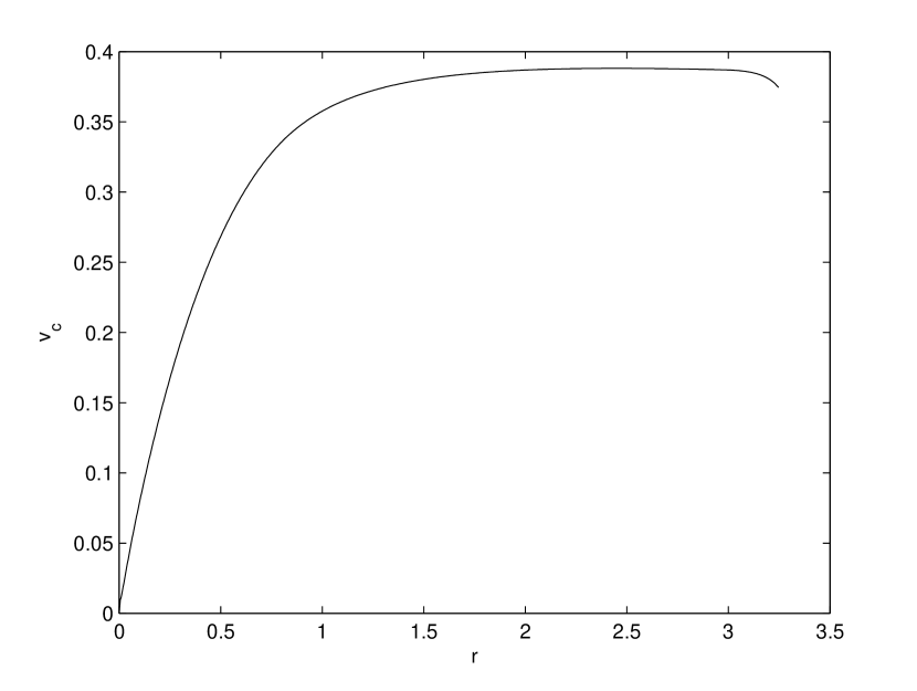
(a) Rotation velocity $v_{c}$ versus radius $r$

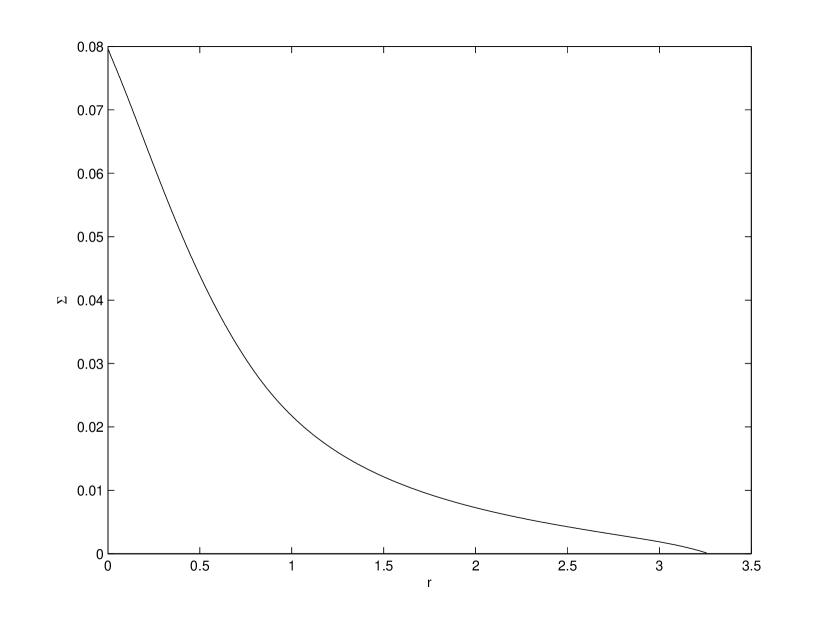
(b) Density $\Sigma$ versus radius $r$

Figure 1: $M=0.3,\;E_{0}=-0.1,\;l=1.0,\;Q=2.0$

We notice that the rotation curve is approximately flat for values of $r$ reaching almost all the way to the boundary of the steady state. The boundary is situated where the mass density vanishes. The potential $U$ for this steady state is depicted in Figure 2.

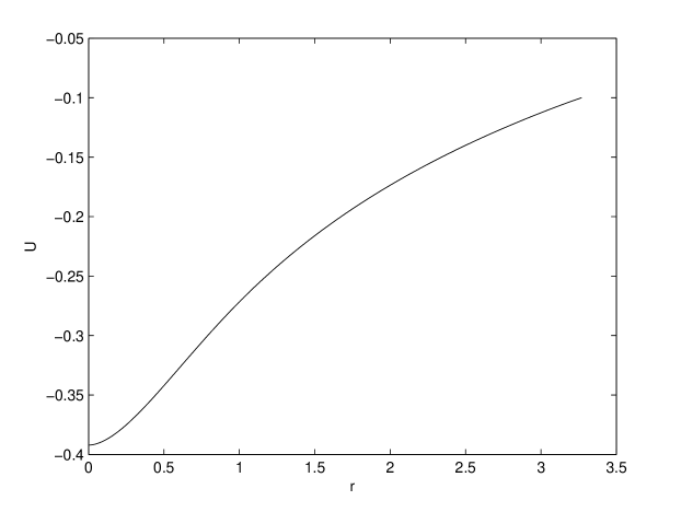
Figure 2: $U$ versus radius $r$ for the steady state in Figure 1

We note that $U=E_{0}$ at the boundary of the steady state. In most cases we omit the potential $U$, since its features are quite similar in the situations we study, but important exceptions are given below where $U$ is not monotone. In Figure 3 and Figure 4 we show the behavior of the rotational velocity and the mass density when the parameter $Q$ is varied for the case in Figure 1.

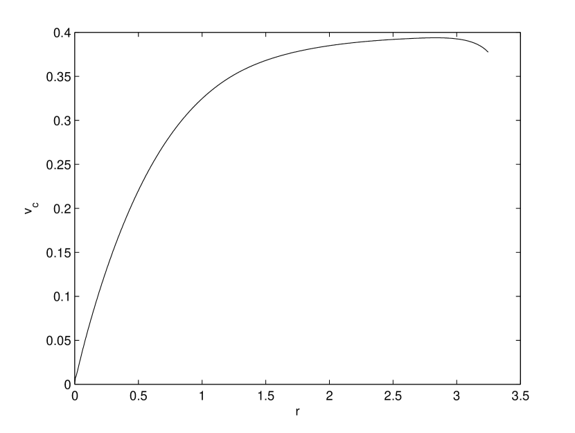
(a) Rotation velocity $v_{c}$ versus radius $r$

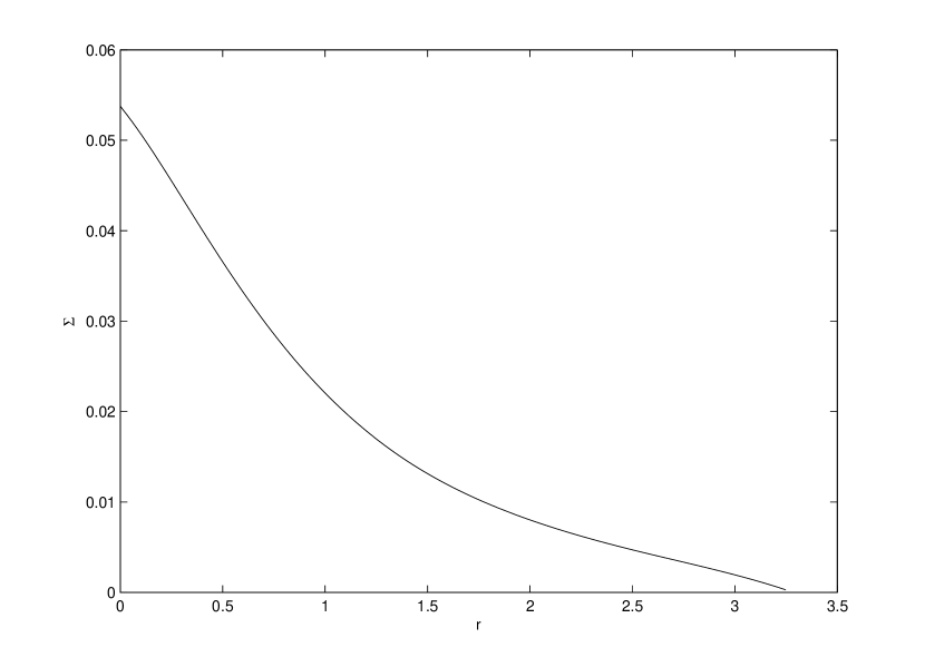
(b) Density $\Sigma$ versus radius $r$

Figure 3: $M=0.3,\;E_{0}=-0.1,\;l=1.0,\;Q=1.5$

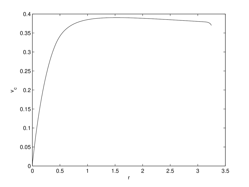
(a) Rotation velocity $v_{c}$ versus radius $r$

(b) Density $\Sigma$ versus radius $r$

Figure 4: $M=0.3,\;E_{0}=-0.1,\;l=1.0,\;Q=3.0$

We notice that the rotation velocity can be slightly increasing or slightly decreasing in a large fraction of the support. It is of course interesting to compare the shape of the rotation curves to data from observations, cf. e.g. (Fuchs 2001, Verheijen & Sancisi 2001, Gentile et al 2004, Salucci 2007, Blok et al 2008, Roos 2010). We find that the shape of the rotation curves in Figures 1, 3, and 4 agrees nicely with the shape of the rotation curves obtained in observations. In the next section we give in fact examples from real galaxies and we find solutions that match the observations very well.

Before studying the effect of changing the parameter $l$ we note that the parameters $M$ (reflected by the choice of $A$) and $E_{0}$ affect the support and amplitude of $v_{c}$ and $\Sigma$. In Figure 5 we again obtain an approximately flat rotation curve, but in this case the support extends further out and the mass is larger.

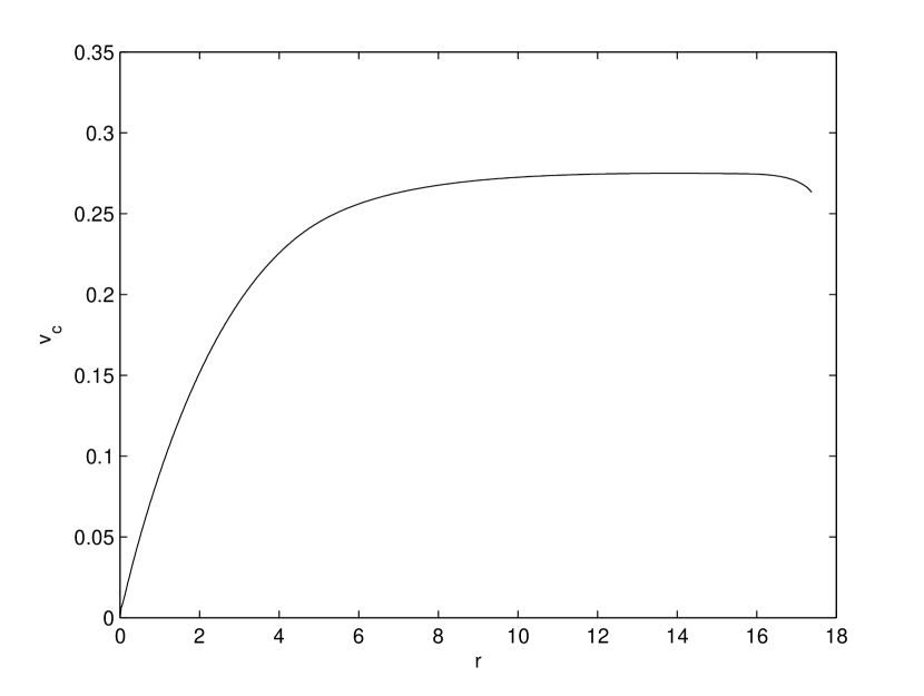
(a) Rotation velocity $v_{c}$ versus radius $r$

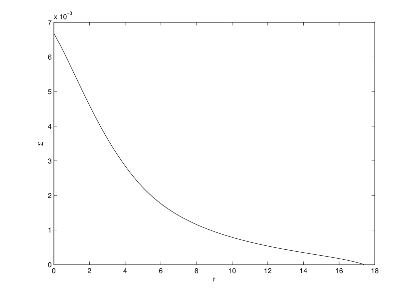
(b) Density $\Sigma$ versus radius $r$

Figure 5: $M=0.8,\;E_{0}=-0.05,\;l=1.0,\;Q=0.5$

We point out that this change does effect the slope of the curve if $Q$ is kept unchanged but in Figure 5 $Q$ has been modified to $Q=0.5$.

The influence of varying the parameter $l$ is studied in Figures 1, 6, and 7, where $l=1,0,-0.75$ respectively.

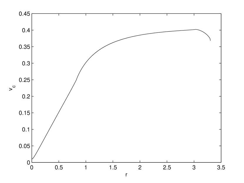
(a) Rotation velocity $v_{c}$ versus radius $r$

(b) Density $\Sigma$ versus radius $r$

Figure 6: $M=0.3,\;E_{0}=-0.1,\;l=0.0,\;Q=2.0$

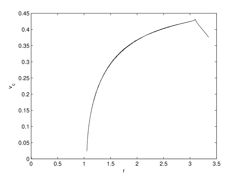
(a) Rotation velocity $v_{c}$ versus radius $r$

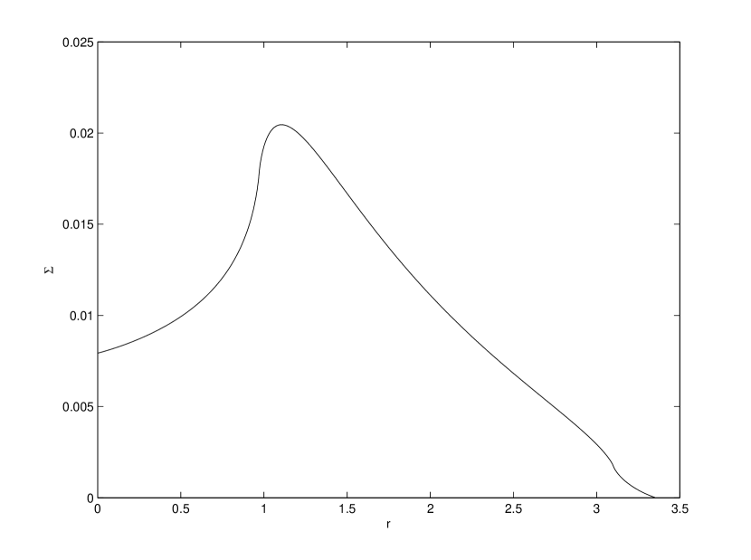
(b) Density $\Sigma$ versus radius $r$

Figure 7: $M=0.3,\;E_{0}=-0.1,\;l=-0.75,\;Q=2.0$

We notice that when $l$ is decreased from $l=1$ to $l=0$ the regularity of the graphs for $v_{c}$ and $\Sigma$ are affected and the slope of the rotation curve increases. When $l$ is decreased further to $l=-0.75$ this effect is more pronounced. In particular neither the density $\Sigma$ in Figure 7 nor the potential $U$ in Figure 8 are monotone.

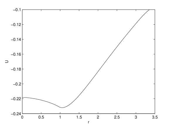
Figure 8: $U$ versus radius $r$ for the steady state in Figure 7

In the domain where $U^{\prime}(r)<0$, $v_{c}$ is not defined which is clear from Figure 7(a). Recall that in the spherically symmetric case the potential is always increasing so the non-monotonicity of $U$ is a particular feature of the axially symmetric Vlasov-Poisson system. A similar example is given in Figures 9 and 10, where $Q$ has been changed so that the rotation curve is approximately flat.

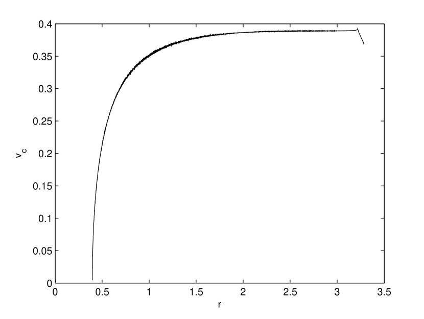
(a) Rotation velocity $v_{c}$ versus radius $r$

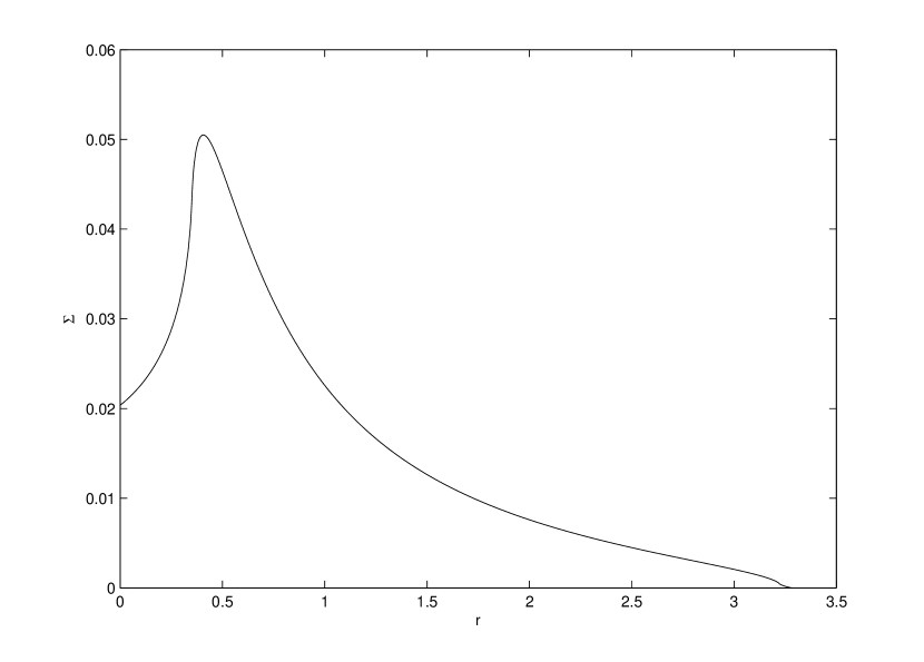
(b) Density $\Sigma$ versus radius $r$

Figure 9: $M=0.3,\;E_{0}=-0.1,\;l=-0.75,\;Q=4.1$

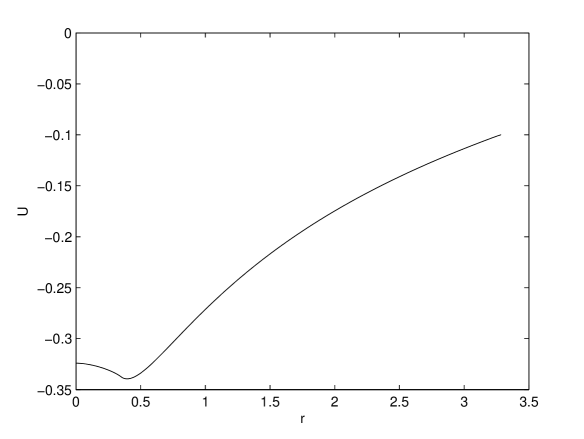
Figure 10: $U$ versus radius $r$ for the steady state in Figure 9

In Theorem 3.1 it was shown that there are no stars in circular orbits in the neighborhood of the boundary of the steady state, cf. however the remark following the theorem. Numerically it is straightforward to compute the range where stars in circular orbits do not exist. By following the proof of Theorem 3.1 it is found that particles in circular orbits do not exist if

$$\Gamma:=E_{0}-\frac{1}{2}r\,U^{\prime}(r)-U(r)<0.$$

For the steady state given in Figure 1 $\Gamma$ is depicted in Figure 11.

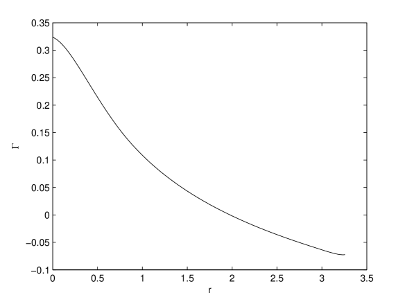
Figure 11: $\Gamma$ versus radius $r$ for the case in Figure 1

In this case $R_{b}=3.26$ and $\Gamma$ is negative for $r>1.98$. On circular orbits in the range $[1.98,3.36]$, i.e., in the range $[0.6R_{b},R_{b}]$, there are no particles in the particle distribution given by $f$. Hence, in the outer 40% of the galaxy there are no stars on circular orbits. Similarly, Figure 12 shows $\Gamma$ for the steady state in Figure 9.

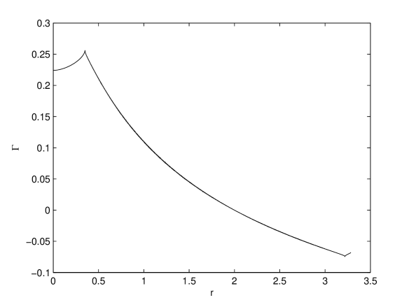
Figure 12: $\Gamma$ versus radius $r$ for the case in Figure 9

In this case $R_{b}=3.28$ and we find that there are no stars on circular orbits in the range $[2.0,3.28]$, i.e., in $[0.61R_{b},R_{b}]$. Since we find in Figure 9 that $U^{\prime}<0$ for $r\leq 0.4$, there are of course no circular orbits at all when $r\leq 0.4$, i.e., for $r\in[0,0.12R_{b}]$.

For the figures above we used Eqn. (3.1) to define the circular velocity $v_{c}(r)$ at radius $r$. In the context of our model it is natural to compute the averaged tangential velocity of the stars from the phase space density $f$ instead, i.e.,

$$\langle v_{\mathrm{tan}}(r)\rangle=\frac{1}{\Sigma(r)}\int_{\mathbb{R}^{2}}v_{\mathrm{tan}}f\,dv,$$

where $v_{\mathrm{tan}}=(x_{1}v_{2}-x_{2}v_{1})/r=L_{z}/r$ is the tangential component of the velocity of a particle at $x$ with velocity $v$. It turns out that for the steady states we constructed this quantity behaves quite differently from $v_{c}$. As an example we plot $\langle v_{\mathrm{tan}}(r)\rangle$ for the steady state shown in Figure 1, cf. Figure 13(a).

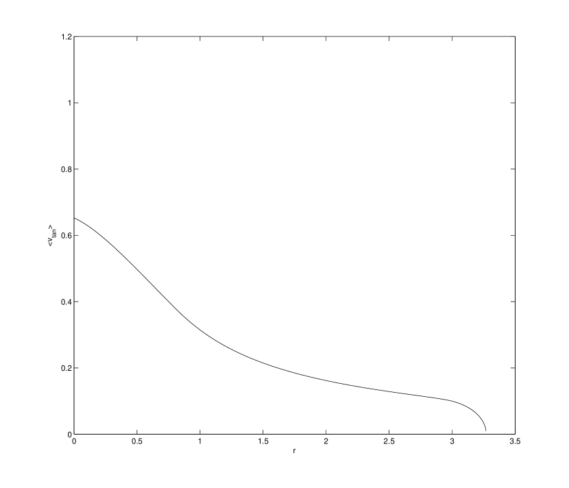
(a) $\langle v_{\mathrm{tan}}\rangle$ versus radius $r$

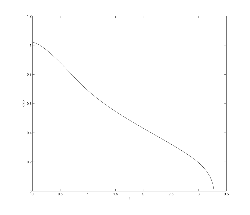
(b) $\langle|v|\rangle$ versus radius $r$

Figure 13: $M=0.3,\;E_{0}=-0.1,\;l=1.0,\;Q=2.0$

We also plot the average of $|v|$, and we observe that both quantities behave quite differently from $v_{c}$. This is in line with Theorem 3.1. As noted in the remark after this theorem the observed rotation curves often seem to be derived from the motion of the interstellar gas, in particular this is the case for the data which we try to fit in Section 6. Two possibilities for resolving the discrepancy between the behaviour of $\langle v_{\mathrm{tan}}\rangle$ and of $v_{c}$ in our models come to mind. One possibility is to add a second particle species to the model which is to represent the gas and from which the averaged tangential velocity $\langle v_{\mathrm{tan}}\rangle$ would then be computed. Another possibility is to search for ansatz functions for which the difference between $\langle v_{\mathrm{tan}}\rangle$ and $v_{c}$ is small. Both possibilities are currently under investigation. It is of interest to note from Figure 13 that in the central part of the particle distribution we construct there are stars which move fast compared to the rotation velocity $v_{c}$ and which in particular move on excentric orbits. In view of the stability of flat galaxies this may be a positive feature of the model, cf. (Kalnajs 1976).

An interesting question is how much mass is needed to obtain the circular rotation velocities in the outer region of the steady state if a Keplerian approach is used. Consider for instance the case depicted in Figure 1. At $r=3.0$ we have from the numerical simulation that $m(3.0)=0.295$, and $v_{c}=0.39$. The mass $M_{K}$ required to obtain $v_{c}=0.39$ using the Kepler formula

$$v_{c}^{2}=\frac{M_{K}}{r},$$

is thus, in this case, $M_{K}=rv_{c}^{2}=0.46$. Hence,

$$\frac{M_{K}}{m(3.0)}=\frac{0.46}{0.295}=1.56,$$

which implies that more than 50% additional mass is required to explain the rotation curve obtained in Figure 1. Analogously, for the steady state in Figure 7, $v_{c}=0.43$ at $r=3.0$, and $m(3.0)=0.29$, which implies that $M_{K}=0.56$ and

$$\frac{M_{K}}{m(3.0)}=\frac{0.56}{0.29}=1.93,$$

so that more than 90% additional mass is required using the Kepler formula.

6 Comparison to observations

In this section we consider data for some of the spiral galaxies studied by Verheijen & Sancisi (2001) which belong to the Ursa Major cluster. The aim is to find solutions of the flat Vlasov-Poisson system which match these data.

In the introduction we stated the Vlasov-Poisson system in dimensionless form, but in order to compare our results with observations we need to attach proper units. Since the gravitational constant $G$ is the only physical constant which enters the system and since we normalized this to unity in (1.2) we can choose any set of units for time, length, and mass in which the numerical value for $G$ equals unity. When we then try to fit the numerical predictions to the observations of a certain galaxy we first choose the unit for length such that the numerically obtained value for its radius corresponds to the observed radius. Then we choose the unit of time (and hence velocity) in such a way that the numerically predicted rotation curve fits the observations—of course this only works if the mathematical model we consider produces a rotation curve with the proper shape, which we try to achieve by varying the parameters in the ansatz (4.1). Once the units for length and time are chosen in this way, the condition $G=1$ fixes the unit for mass, and we can for example transform the numerically obtained value for the mass into a predicted mass of the galaxy under consideration in units of solar masses.

In the pictures below we have normalized the radius so that the boundary occurs at $r=1$. However, we choose not to identify the radius of the last observation, i.e., the largest radius of the observational data, with the boundary of the support $R_{b}$ of a solution since the density vanishes at the boundary. Instead we identify it with a radius clearly within the support and we choose to identify it with $\lambda R_{b}$, where $\lambda\approx 0.96$.

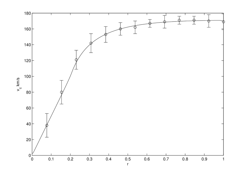
Figure 14: The galaxy NGC3877. Observational data (circles) and VP solution (solid line).

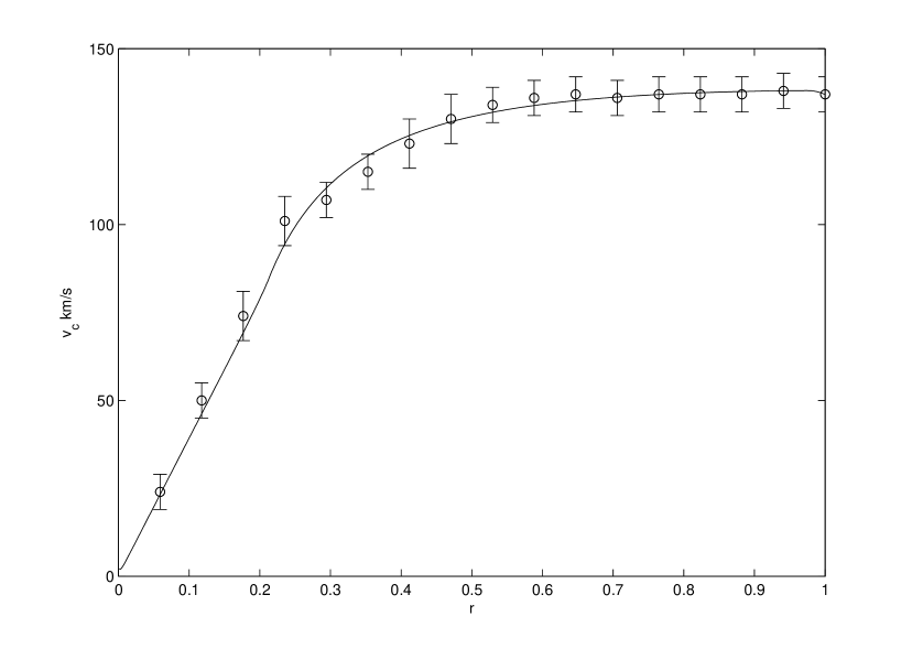
Figure 15: The galaxy NGC3917. Observational data (circles) and VP solution (solid line).

The measured rotation curves for the galaxies NGC3877, NGC3917, NGC3949, and NGC4010 are depicted by open circles in Figures 14, 15, 16, and 17 respectively. The uncertainties in the observational data are tabulated in (Verheijen & Sancisi 2001) and are shown as error bars.

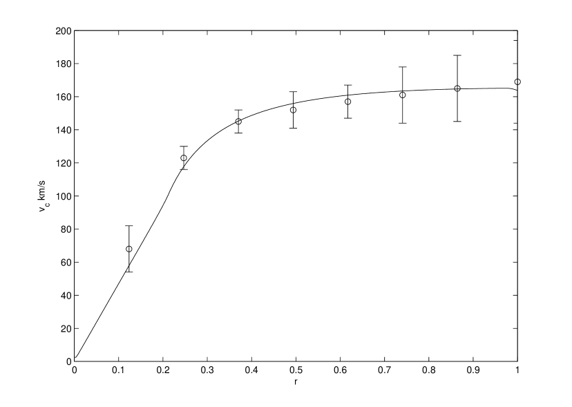
Figure 16: The galaxy NGC3949. Observational data (circles) and VP solution (solid line).

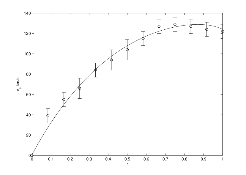
Figure 17: The galaxy NGC4010. Observational data (circles) and VP solution (solid line).

The solid curve in each of these figures is the rotation curve given by the solution of the flat Vlasov-Poisson system using the ansatz (4.1). The solution is then scaled by the procedure described above. The parameter values in the ansatz (4.1) are as follows. In all the four cases $k=0,M=0.3$ and $E_{0}=-0.1$. In Figure 14 $l=0$ and $Q=2.40$, in Figure 15 $l=0$ and $Q=2.30$, in Figure 16 $l=0$ and $Q=2.35$, and in Figure 17 $l=1$ and $Q=0.65$. Taking into account the uncertainties of the observational data we conclude that the solutions agree very well with the observations.

As explained above we can predict the total mass of these galaxies from the numerical results, and the corresponding predictions are tabulated in Table 1.

galaxy	predicted mass
	in solar masses
NGC3877	$4.7\cdot 10^{10}M_{\odot}$
NGC3917	$4.0\cdot 10^{10}M_{\odot}$
NGC3949	$3.5\cdot 10^{10}M_{\odot}$
NGC4010	$2.2\cdot 10^{10}M_{\odot}$

Table 1: Predicted masses

The masses we obtain agree well with the ones obtained by González, Plata & Ramos-Caro (2010) with a completely different fitting approach.

Acknowledgements. The authors sincerely thank an anonymous referee for several very helpful and constructive suggestions. They also thank Roman Firt for teaching them how to use the gsl package for computing the elliptic integral in equation (2.2), and Markus Kunze for pointing out the reference (Dejonghe 1986). The material presented here is based on work supported by the National Science Foundation under Grant No. 0932078 000, while the first author was in residence at the Mathematical Sciences Research Institute in Berkeley, California, during the fall of 2013. The first author wants to express his gratitude for the invitation to MSRI.

References

Amorisco N. C., Bertin G., 2010, AIP, 1242, 288

Batt J., Faltenbacher W., Horst E., 1986, Arch. Rat. Mech. Anal., 93, 159

Binney J., Tremaine S., 1987, Galactic Dynamics, Princeton Univ. Press, Princeton, NJ

Blok W. J. G de, Walter F., Brinks E., Trachternach C., Oh S.-H., Kennicutt R. C. Jr., 2008, Astron. J., 136, 2648

Bosma A., 1981, Astron. J., 86, 1825

Chavanis P. H., 2003, A&A, 401, 15

Dejonghe H., 1986, Physics reports, 133, 217

Famaey B., McGaugh S. S., 2012, Living Rev. Relativity, 15

Firt R., Rein G., 2006, Analysis, 26, 507

Fuchs B., 2001, Dark Matter in Astro- and Particle Physics. Proc. Int. Conf. DARK 2000, Heidelberg, p. 25

Gentile G., Salucci P., Klein U., Vergani D., Kalberla P., 2004, MNRAS, 351, 903

González G. A., Plata S. M. , Ramos-Caro J., 2010, MNRAS, 404, 468

Huré J.-M., 2005, A& A, 434, 1

Kalnajs A. J., 1972, Astrophys. J., 175, 63

Kalnajs A. J., 1976, Astrophys. J., 205, 751

Lynden-Bell D., 1967, MNRAS, 136, 101

Moffat J. W., 2006, J. of Cosmology and Astroparticle Physics, 03, 004

Nguyen P. H., Lingam M.,2013, MNRAS, 436, 2014

Pedraza J. F., Ramos-Caro J., González G. A.,2008, MNRAS, 390, 1587

Ramming T., Rein G., 2013, SIAM J. Math. Anal., 45, 900

Ramos-Caro J., Agn C. A., Pedraza J. F., 2012, Phys. Rev. D, 86, 043008

Rein G., 2007, in Dafermos C. M., Feireisl E., eds, Handbook of Differential Equations, Evolutionary Equations, 3

Rein G., 1999, Commun. Math. Phys., 205, 229

Rein G., 2013, preprint (arXiv:1312.3765)

Rein G., Rendall A. D., 2000, Math. Proc. Camb. Phil. Soc., 128, 363

Rodrigues D. C., Letelier P. S., Shapiro I. L., 2010, J. of Cosmology and Astroparticle Physics, 04, 020

Roos M., 2010, preprint (arXiv:1001.0316)

Rubin V. C., Ford J., Thonnard W. K., Burnstein D., 1982, Astron. Rep., 261, 439

Salucci P., 2007, Proc. IAU, 244, 53

Schulz E., 2012, Astrophys. J., 747, 106

Verheijen M. A. Sancisi R., 2001, A& A, 370, 765