Single-index modulated multiple testing

Abstract

In the context of large-scale multiple testing, hypotheses are often accompanied with certain prior information. In this paper, we present a single-index modulated (SIM) multiple testing procedure, which maintains control of the false discovery rate while incorporating prior information, by assuming the availability of a bivariate $p$-value, $(p_{1},p_{2})$, for each hypothesis, where $p_{1}$ is a preliminary $p$-value from prior information and $p_{2}$ is the primary $p$-value for the ultimate analysis. To find the optimal rejection region for the bivariate $p$-value, we propose a criteria based on the ratio of probability density functions of $(p_{1},p_{2})$ under the true null and nonnull. This criteria in the bivariate normal setting further motivates us to project the bivariate $p$-value to a single-index, $p(\theta)$, for a wide range of directions $\theta$. The true null distribution of $p(\theta)$ is estimated via parametric and nonparametric approaches, leading to two procedures for estimating and controlling the false discovery rate. To derive the optimal projection direction $\theta$, we propose a new approach based on power comparison, which is further shown to be consistent under some mild conditions. Simulation evaluations indicate that the SIM multiple testing procedure improves the detection power significantly while controlling the false discovery rate. Analysis of a real dataset will be illustrated.

and t1Supported by NSF Grants DMS-11-06586 and DMS-13-08872, and Wisconsin Alumni Research Foundation.

1 Introduction

Large-scale simultaneous hypothesis testing problems, with thousands or even tens of thousands of cases considered together, have become a familiar feature in scientific fields such as biology, medicine, genetics, neuroscience, economics and finance. For example, in genome-wide association study, testing for association between genetic variation and a complex disease typically requires scanning hundreds of thousands of genetic polymorphisms; in functional magnetic resonance imaging ($\mathrm{fMRI}$), time-course measurements over $10^{4}$–$10^{5}$ voxels in the brain are typically available to allow investigators to determine which areas of the brain are involved in a cognitive task. Multiple testing procedures, especially the false discovery rate ($\mathrm{FDR}$) control method BenjaminiHochberg1995 , have been widely used to screen the massive data sets to identify a few interesting cases.

In many real-world applications, the tests are accompanied with a scientifically meaningful structure. In $\mathrm{fMRI}$, each test corresponds to a specific brain location; in microarray studies, each test is related to a specific gene. These types of structural information usually provide valuable prior information. For example, previous studies may suggest that some null hypotheses are more or less likely to be false; similarly, in spatially-structured problems, nonnull hypotheses are more likely to be clustered than true nulls. It is thus anticipated that exploiting structural prior information will improve the performance of conventional multiple testing procedures. Several attempts have been made in the literature to incorporate prior information. For instance, methods that up-weight or down-weight hypotheses appeared in BenjaminiHochberg1997 , Genoveseetal2006 and HuZhaoZhou2010 . A comprehensive review of weighted hypothesis testing can be found in RoederWasserman2009 and the references therein. A different approach, based on a two-stage approach mainly arising from the microarray literature Bourgonetal2010 , HackstadtHess2009 , Lusaetal2008 , McClintickEdenberg2006 , Talloenetal2007 , Tritchleretal2009 , extracted the prior information to remove a subset of genes which seem to generate uninformative signals in the filtering stage, followed by applying some multiple testing procedure to the remaining genes which have passed the filter in the selection stage.

Very little work, however, has been published on theoretically quantifying the extent to which the pair of filter and test statistics in the above two-stage procedure, as well as the pair of random weight and test statistics in weighted hypothesis testing affect $\mathrm{FDR}$ and power. This issue is critically important, because arbitrarily choosing a filter (or weight) statistic may lead to loss of type I error control. To guarantee the validity of filtering in the two-stage multiple testing procedure, Bourgonetal2010  recommended the use of a filter statistic (i.e., overall sample variance) which is independent of the test statistic to reduce the impact that multiple testing adjustment has on detection power. Analogously, the weight and test statistics are assumed to be independent in the literature of weighted hypothesis testing. However, questions always arise about (I) the adequacy of the independence assumption between the filter (or weight) and test statistics, and (II) the subjectiveness in setting the proportion of hypotheses to be removed in the filtering stage.

We intend to incorporate the prior information into large-scale multiple testing, via a proposed single-index modulated ($\mathrm{SIM}$) multiple testing procedure. This inspires us to study a bivariate $p$-value $(p_{i1},p_{i2})$ for each of the $i$th hypothesis, $i=1,\ldots,m$, where $m$ is the number of hypotheses, $p_{i1}$ is the preliminary $p$-value from the prior information (e.g., the filter or weight), and $p_{i2}$ is the primary $p$-value for the ultimate analysis (from the test statistic). Unlike Bourgonetal2010 and Genoveseetal2006 , we do not impose the independence assumption between the filter (or weight) and test statistics. This greatly broadens the scope of filters (or weights) that can be chosen. Moreover, we wish to point out that Chi2008 explored a $\mathrm{FDR}$ procedure which can achieve the control of $\mathrm{FDR}$ with asymptotically maximum power through nested regions of multivariate $p$-values of test statistics. However, that approach assumed independence between components in each multivariate $p$-value under true null hypotheses, thus is not directly applicable to our study.

In our approach, the bivariate $p$-value in multiple testing is projected into a single-index, $p(\theta)$, where the direction $\theta$ takes value in the interval $[0,\pi/2]$. Due to the projection, the true null distribution of the single-index $p(\theta)$ is no longer uniform and thus needs to be estimated. We propose a parametric and a nonparametric approach to estimate it. A data-driven estimator based on power comparison is developed for the optimal projection direction $\theta$. This estimator is further shown to be consistent under some mild conditions. The resulting method leads to the estimation and control of $\mathrm{FDR}$ for the $\mathrm{SIM}$ multiple testing procedure. Compared with the conventional multiple testing procedure which ignores the prior information, the $\mathrm{SIM}$ multiple testing procedure can improve the detection power substantially as long as components in the bivariate $p$-value are not highly positively correlated. Extensive simulation studies support the validity and detection power of our approach. Analysis of a real dataset illustrates the practical utility of the proposed $\mathrm{SIM}$ procedure.

The rest of the paper is organized as follows. Section 2 reviews the conventional multiple testing procedure, and outlines the proposed $\mathrm{SIM}$ multiple testing procedure. Section 3 supplies theoretical derivation of the $\mathrm{SIM}$ multiple testing procedure. Section 4 presents methods for estimating and controlling $\mathrm{FDR}$ used in the $\mathrm{SIM}$ multiple testing procedure and Section 5 investigates their theoretical properties. Section 6 evaluates the performance of the proposed procedure in simulation studies. Section 7 analyzes a real dataset. Section 8 ends the paper with a brief discussion. All technical proofs are relegated to Appendices A and B.

2 Overview of the single-index modulated multiple testing procedure

2.1 Review of the conventional multiple testing procedure

For the sake of discussion, we begin with a brief review of the conventional multiple testing procedure. For testing a family of null hypotheses, $\{H_{0}(i)\}_{i=1}^{m}$, with the corresponding $p$-values $\{p_{1},\ldots,p_{m}\}$, Table 1 describes the outcomes when applying some significance rule, which means rejecting null hypotheses with corresponding $p$-values less than or equal to some threshold. The false discovery rate ($\mathrm{FDR}$), $\mathrm{FDR}=E(\frac{V}{R\vee 1})$, depicts the expected proportion of incorrectly rejected null hypotheses BenjaminiHochberg1995 , where $R\vee 1=\max\{R,1\}$. An empirical process definition of $\mathrm{FDR}$,

$$\mathrm{FDR}(t) = E\biggl{\{}\frac{V(t)}{R(t)\vee 1}\biggr{\}},\qquad t\in[0,1],$$

was introduced by Storeyetal2004 , where $V(t)=\#\{\mbox{true null }p_{i}\dvtx p_{i}\leq t\}$, and $R(t)=\#\{p_{i}\dvtx p_{i}\leq t\}$.

=250pt Retain null Reject null Total Null is true $U$ $V$ $m_{0}$ Nonnull is true $T$ $S$ $m_{1}$ Total $W$ $R$ $m$

Table 1: Outcomes from testing $m$ null hypotheses based on a significance rule

Compared with the frequentist framework of $\mathrm{FDR}$, $\mathrm{FDR}$ methods also have a Bayesian rationale in terms of the two-groups model. Let $F_{0}(t)$ and $F_{1}(t)$ be the cumulative distribution functions ($\mathrm{CDF}$) of a $p$-value under the true null and nonnull, respectively, and define $F(t)=\pi_{0}F_{0}(t)+\pi_{1}F_{1}(t)$ as its marginal $\mathrm{CDF}$, where $\pi_{0}=\mathrm{P}$(null is true) and $\pi_{1}=1-\pi_{0}$. Then the Bayes formula yields the posterior probability,

$$\mathrm{Fdr}(t) = \mathrm{P}(\mbox{true null}|p\leq t)=\frac{\pi_{0}F_{0}(t)}{\pi_{0}F_{0}(t)+\pi_{1}F_{1}(t)}=\frac{\pi_{0}F_{0}(t)}{F(t)},$$ (1)

of a null hypothesis being true given that its $p$-value is less than or equal to some threshold $t$.

Assuming that $p$-values under the true null are independent (or weakly dependent) and uniformly distributed on the interval $[0,1]$, Storey2002 proposed a point estimate of $\mathrm{FDR}$ by

$$\widehat{\mathrm{FDR}}(t)=\frac{m\hat{\pi}_{0}t}{R(t)\vee 1}=\frac{\hat{\pi}_{0}t}{\{R(t)\vee 1\}/m}.$$ (2)

For a chosen level $\alpha$, a data-driven threshold for the $p$-values is determined by

$$t_{\alpha}(\widehat{\mathrm{FDR}})=\sup\bigl{\{}0\leq t\leq 1\dvtx\widehat{\mathrm{FDR}}(t)\leq\alpha\bigr{\}}.$$ (3)

Reject a null hypothesis if its $p$-value is less than or equal to $t_{\alpha}(\widehat{\mathrm{FDR}})$. Hereafter, we will refer to (2) as the estimation approach for $\mathrm{FDR}$ and (3) as the controlling approach for $\mathrm{FDR}$.

2.2 Outline of the single-index modulated multiple testing

Before describing the details of our proposed single-index modulated multiple testing, we outline the major idea and methodology. [(a)]

For each bivariate $p$-value $(p_{i1},p_{i2})$, $i=1,\ldots,m$, project it into a sequence of single indices, $\{p_{i}(\theta_{l})\}_{l=1}^{L}$, according to $p_{i}(\theta)=\Phi(\cos(\theta)\Phi^{-1}(p_{i1})+\sin(\theta)\Phi^{-1}(p_{i2}))$, where $\{\theta_{l}\}_{l=1}^{L}$ are equally spaced on the interval $[0,\pi/2]$.

For each $\theta_{l}$, estimate the true null distribution function of $\{p_{i}(\theta_{l})\dvtx i=1,\ldots,m\}$ by $\widehat{F}_{0}(t,\theta_{l})$ using either a parametric or nonparametric approach.

For each $\theta_{l}$, calculate ${R(\hat{t}^{*}_{\alpha^{\prime}}(\theta_{l}),\theta_{l})}$, where $R(t,\theta)={\#\{p_{i}(\theta)\leq t\}}$, and $\hat{t}^{*}_{\alpha^{\prime}}(\theta_{l})=\sup\{0\leq t\leq 1\dvtx{m\widehat{F}_{0}(t,\theta_{l})}/{\{R(t,\theta_{l})\vee 1\}}\leq\alpha^{\prime}\}$, with $\alpha^{\prime}\in(0,1)$. Determine the data-driven optimal projection direction $\hat{\theta}(\alpha^{\prime})=\theta_{L^{*}}$, where $L^{*}=\arg\max_{1\leq l\leq L}R(\hat{t}^{*}_{\alpha^{\prime}}(\theta_{l}),\theta_{l})$.

Estimate the proportion $\pi_{0}$ of true null hypotheses by $\hat{\pi}_{0}$.

For the projected $p$-values $\{p_{i}(\hat{\theta}(\alpha^{\prime}))\dvtx i=1,\ldots,m\}$, set the threshold $\hat{t}_{\alpha}$ to be $\sup\{0\leq t\leq 1\dvtx{m\hat{\pi}_{0}\widehat{F}_{0}(t,\hat{\theta}(\alpha^{\prime}))}/{\{R(t,\hat{\theta}(\alpha^{\prime}))\vee 1\}}\leq\alpha\}$, where $\alpha\in(0,1)$. Reject a null hypothesis $H_{0}(i)$ if the corresponding $p_{i}(\hat{\theta}(\alpha^{\prime}))$ is less than or equal to $\hat{t}_{\alpha}$.

The idea of the single-index projection in part (a) is not straightforward, evolving from Sections 3.1 and 3.2, to Section 3.3. Section 3.1 starts with an intuitive idea of using a rectangular shape of the rejection region for bivariate $p$-values; Section 3.2 derives a general form of optimal rejection region using local false discovery rate EfronTibshirani2002 ; Section 3.3 is motivated from the bivariate normal setting, where the optimal rejection region in Section 3.2 will lead to the projected $p$-value, that is, the single-index $p(\theta)$. The parametric and nonparametric estimators in part (b) will be given in Section 4.2. Incorporating this, the estimator for the proportion of true null hypotheses in part (d) is derived in Section 4.3. The optimal projection direction in part (c) is estimated by a novel approach given in Section 4.4. The procedure in part (e) for estimation and control of the false discovery rate is provided in Section 4.5.

3 Optimal rejection region for bivariate $p$-values

Recall that for univariate $p$-values, the rejection region is an interval $[0,t]$. In this section, we will discuss the rejection region for bivariate $p$-values and its optimal choice.

3.1 Optimal rejection region based on a rectangle

Intuitively, the false discovery rate for the bivariate $p$-values can be defined based on a rectangular rejection region, $[0,t_{1}]\times[0,t_{2}]$. For notational simplicity, let $\mathbf{p}=(p_{1},p_{2})$ denote the bivariate $p$-value, and define $F_{0}(\mathbf{p})$, $F_{1}(\mathbf{p})$ and $F(\mathbf{p})$ to be the true null joint distribution, nonnull joint distribution and joint distribution of $\mathbf{p}$, respectively. Also, let $f_{0}(\mathbf{p})$, $f_{1}(\mathbf{p})$ and $f(\mathbf{p})$ be the corresponding probability density functions (p.d.f.). Then the Bayesian $\mathrm{Fdr}$ for the bivariate $p$-value based on a rectangular rejection region is formulated as

$$\mathrm{Fdr}(\mathbf{t})=\mathrm{P}(\mbox{true null}|\mathbf{p}\leq\mathbf{t})=\frac{\pi_{0}F_{0}(\mathbf{t})}{\pi_{0}F_{0}(\mathbf{t})+\pi_{1}F_{1}(\mathbf{t})},$$ (4)

where $\mathbf{t}=(t_{1},t_{2})$ and $\{\mathbf{p}\leq\mathbf{t}\}$ denotes the event $\{p_{1}\leq t_{1},p_{2}\leq t_{2}\}$. There are infinite choices of rejection regions $[0,t_{1}]\times[0,t_{2}]$ such that $\mathrm{Fdr}(\mathbf{t})\leq\alpha$. A possible criteria to choose ${\mathbf{t}}^{*}=(t_{1}^{*},t_{2}^{*})$ for a best rejection region is based on power comparison. Specifically, that choice is

$$\mathbf{t}^{*}=\arg\max_{\mathbf{t}}\bigl{\{}F_{1}(\mathbf{t})\dvtx\mathrm{Fdr}(\mathbf{t})\leq\alpha\bigr{\}}.$$ (5)

Remark 1.

The Bayesian $\mathrm{Fdr}$ formula (4) can also be derived using conditional probability,

$$\mathrm{Fdr}(\mathbf{t}) = \frac{\mathrm{P}(\mbox{true null}|p_{1}\leq t_{1})\mathrm{P}(p_{2}\leq t_{2}|p_{1}\leq t_{1},\mbox{true null})}{\mathrm{P}(p_{2}\leq t_{2}|p_{1}\leq t_{1})}$$

$$= \frac{\mathrm{Fdr}_{p_{1}}(t_{1})\mathrm{P}(p_{2}\leq t_{2}|p_{1}\leq t_{1},\mbox{true null})}{\mathrm{P}(p_{2}\leq t_{2}|p_{1}\leq t_{1})},$$

where $\mathrm{Fdr}_{p_{1}}(t_{1})=\mathrm{P}(\mbox{true null}|p_{1}\leq t_{1})$. From formula (1), the Bayesian $\mathrm{Fdr}$ for the bivariate $p$-value based on a rectangular rejection region is not simply the product of those with respect to the preliminary $p$-value and primary $p$-value, that is, $\mathrm{Fdr}(\mathbf{t})\neq\mathrm{Fdr}_{p_{1}}(t_{1})\times\mathrm{Fdr}_{p_{2}}(t_{2})$, where $\mathrm{Fdr}_{p_{2}}(t_{2})=\mathrm{P}(\mbox{true null}|p_{2}\leq t_{2})$. Furthermore, formula (1) provides an insight into the two-stage multiple testing in Bourgonetal2010 if $p_{1}$ is utilized as the filter in the filtering stage and $p_{2}$ is obtained from a test statistic in the selection stage. Comparing (1) with (1), we find that $\mathrm{Fdr}_{p_{1}}(t_{1})$ in the filtering stage is the proportion of the true null hypotheses served in the selection stage. On the one hand, in order to improve the power in the selection stage, we can control $\mathrm{Fdr}_{p_{1}}(t_{1})$ to be small. On the other hand, increasing $\mathrm{Fdr}_{p_{1}}(t_{1})$ will assure that we do not screen out too many nonnull hypotheses from the filtering stage.

3.2 General form of optimal rejection region

In Section 3.1, we observe that among infinite choices of rectangular rejection regions $[0,t_{1}]\times[0,t_{2}]$ such that the Bayesian $\mathrm{Fdr}$ is less than or equal to $\alpha$, there exists one “best” rectangle $[0,t_{1}^{*}]\times[0,t_{2}^{*}]$ with highest power. In this section, we seek a general form of optimal rejection region, by relaxing the shape of rejection region. Let $\mathbf{S}$ denote a rejection region. Following (4), the Bayesian $\mathrm{Fdr}$ can be generalized to

$$\mathrm{Fdr}(\mathbf{S})=\mathrm{P}(\mbox{true null}|\mathbf{p}\in\mathbf{S})=\frac{\pi_{0}F_{0}(\mathbf{S})}{\pi_{0}F_{0}(\mathbf{S})+\pi_{1}F_{1}(\mathbf{S})},$$ (7)

where $F_{j}(\mathbf{S})=\int_{\mathbf{S}}f_{j}(\mathbf{p})\,d\mathbf{p}$, $j=0,1$. An optimal rejection region $\mathbf{S}^{*}$ is based on the following definition:

$$\mathbf{S}^{*}=\arg\max_{\mathbf{S}}\bigl{\{}F_{1}(\mathbf{S})\dvtx\mathrm{Fdr}(\mathbf{S})\leq\alpha\bigr{\}}.$$ (8)

Note that (5) is a special case of (8), by restricting $\mathbf{S}$ to be rectangular.

Proposition 1.

Assume the two-groups model holds for the bivariate $p$-values and let $\mathrm{fdr}(\mathbf{p})=\pi_{0}f_{0}(\mathbf{p})/\{\pi_{0}f_{0}(\mathbf{p})+\pi_{1}f_{1}(\mathbf{p})\}$ be the generalization of local false discovery rate; see EfronTibshirani2002 and Efronetal2001 . Further suppose that for any constant $C_{0}$,

$$\mathrm{P}\bigl{(}\mathbf{p}\dvtx\mathrm{fdr}(\mathbf{p})=C_{0}\bigr{)}=0.$$ (9)

Denote by $\mathbf{S}_{\mathrm{OR}}$ the rejection region to be formed by $\mathbf{S}_{\mathrm{OR}}=\{\mathbf{p}\dvtx\mathrm{fdr}(\mathbf{p})\leq C\}$, where $C$ is a constant such that $\mathrm{Fdr}(\mathbf{S}_{\mathrm{OR}})=\alpha$. Then for any rejection region $\mathbf{S}$ satisfying $\mathrm{Fdr}(\mathbf{S})\leq\alpha$, we have $F_{1}(\mathbf{S})\leq F_{1}(\mathbf{S}_{\mathrm{OR}})$.

From Proposition 1, the general form of optimal rejection region (8) can be equivalently described as follows: within the rejection region $\mathbf{S}^{*}$, the local false discovery rate $\mathrm{fdr}(\mathbf{p})$ should be less than or equal to some threshold, which is equivalent to setting ${f_{1}(\mathbf{p})}/{f_{0}(\mathbf{p})}$ to be larger than or equal to some threshold. Thus, we propose the optimal rejection region (8) to be formed by

$$\mathbf{S}^{*}=\bigl{\{}\mathbf{p}\dvtx f_{1}(\mathbf{p})/f_{0}(\mathbf{p})\geq C\bigr{\}},$$ (10)

where $C$ is a constant such that $\mathrm{Fdr}(\mathbf{S}^{*})=\alpha$.

Remark 2.

In traditional hypothesis testing, the Neyman–Pearson lemma indicates that the rejection region of the uniformly most powerful (UMP) test is in the form of likelihood ratio of test statistics if both the null and nonnull hypotheses are simple. Hence, the form of the optimal rejection region $\mathbf{S}^{*}$ using local false discovery rate is similar to that derived from the UMP test. (10) is also a homogeneous version of the optimal discovery procedure proposed by Storey2007 , where the null and nonnull distributions across the tests are less homogeneous and strongly correlated.

3.3 Optimal rejection region under bivariate normality

In this subsection, we will first derive the true null and nonnull distributions of a bivariate $p$-value under bivariate normality, followed by approximating the shape of the optimal rejection region using criteria (10).

Efron Efron2007 introduced a $z$-value $(\Phi^{-1}(p))$ into traditional multiple testing problem and assumed that the empirical null distribution of $z$-value is normal with mean $\mu$ and standard deviation $\sigma$. To derive an explicit form of the true null distribution of $\mathbf{p}$, we borrow the idea of empirical null distribution in Efron2007 and make extension to the case of bivariate $p$-values, assuming the bivariate normality as follows:

Under the true null hypothesis, the transformed $p$-value $(\Phi^{-1}(p_{1}),\break\Phi^{-1}(p_{2}))$ follows a bivariate normal distribution $\mathcal{N}({\bolds{\mu}}_{0},\Sigma_{0})$, where

$${\bolds{\mu}}_{0}=(\mu_{0;1},\mu_{0;2})^{T},\qquad\Sigma_{0}=\pmatrix{\sigma_{0;1}^{2}&\rho_{0}\sigma_{0;1}\sigma_{0;2}\vspace*{3pt}\cr\rho_{0}\sigma_{0;1}\sigma_{0;2}&\sigma_{0;2}^{2}}.$$ (11)

Under the nonnull, the transformed $p$-value $(\Phi^{-1}(p_{1}),\Phi^{-1}(p_{2}))$ also follows a bivariate normal distribution $\mathcal{N}({\bolds{\mu}}_{1},\Sigma_{1})$, where

$${\bolds{\mu}}_{1}=(\mu_{1;1},\mu_{1;2})^{T},\qquad\Sigma_{1}=\pmatrix{\sigma_{1;1}^{2}&\rho_{1}\sigma_{1;1}\sigma_{1;2}\vspace*{3pt}\cr\rho_{1}\sigma_{1;1}\sigma_{1;2}&\sigma_{1;2}^{2}}.$$ (12)

Remark 3.

The assumption (N1) is strictly satisfied if the components of bivariate $p$-value are independent under the true null. For the dependence case, this assumption is approximately true. As a specific example, (N1) holds if the preliminary test statistic and primary test statistic (bivariate test statistic) under the true null follows a bivariate normal distribution for one-sided hypotheses; see (B) in Appendix B. The assumption (N2) is not required for the general theory in Section 5 and only serves as a motivation for developing the proposed rejection region (16).

If (N1) and (N2) hold, some algebraic calculations yield the densities of $\mathbf{p}$ under the true null and nonnull,

$$\qquad f_{0}(\mathbf{p}) = \frac{1}{\sigma_{0;1}\sigma_{0;2}\sqrt{1-\rho_{0}^{2}}}\exp\biggl{(}\frac{\{\Phi^{-1}(p_{1})\}^{2}+\{\Phi^{-1}(p_{2})\}^{2}}{2}\biggr{)}$$

$${}\times\exp\biggl{(}-\biggl{(}\biggl{\{}\frac{\Phi^{-1}(p_{1})-\mu_{0;1}}{\sigma_{0;1}}\biggr{\}}^{2}+\biggl{\{}\frac{\Phi^{-1}(p_{2})-\mu_{0;2}}{\sigma_{0;2}}\biggr{\}}^{2}$$

$$\hskip 49.0pt{}-2\rho_{0}\biggl{\{}\frac{\Phi^{-1}(p_{1})-\mu_{0;1}}{\sigma_{0;1}}\biggr{\}}\biggl{\{}\frac{\Phi^{-1}(p_{2})-\mu_{0;2}}{\sigma_{0;2}}\biggr{\}}\biggr{)}$$

$$\hskip 197.5pt{}\Big{/}\bigl{(}{2\bigl{(}1-\rho_{0}^{2}\bigr{)}}\bigr{)}\biggr{)},$$

$$f_{1}(\mathbf{p}) = \frac{1}{\sigma_{1;1}\sigma_{1;2}\sqrt{1-\rho_{1}^{2}}}\exp\biggl{(}\frac{\{\Phi^{-1}(p_{1})\}^{2}+\{\Phi^{-1}(p_{2})\}^{2}}{2}\biggr{)}$$

$${}\times\exp\biggl{(}-\biggl{(}\biggl{\{}\frac{\Phi^{-1}(p_{1})-\mu_{1;1}}{\sigma_{1;1}}\biggr{\}}^{2}+\biggl{\{}\frac{\Phi^{-1}(p_{2})-\mu_{1;2}}{\sigma_{1;2}}\biggr{\}}^{2}$$

$$\hskip 49.0pt{}-2\rho_{1}\biggl{\{}\frac{\Phi^{-1}(p_{1})-\mu_{1;1}}{\sigma_{1;1}}\biggr{\}}\biggl{\{}\frac{\Phi^{-1}(p_{2})-\mu_{1;2}}{\sigma_{1;2}}\biggr{\}}\biggr{)}$$

$$\hskip 198.0pt{}\Big{/}\bigl{(}2\bigl{(}1-\rho_{1}^{2}\bigr{)}\bigr{)}\biggr{)}.$$

By combining (3.3) with the criteria (10), the optimal rejection region under bivariate normality takes the form

$$\mathbf{S}^{*}=\bigl{\{}\mathbf{p}\dvtx{\mathbf{Z}}^{T}{\bolds{\beta}}\geq C\bigr{\}},$$ (14)

with a constant $C$ such that $\mathrm{Fdr}(\mathbf{S}^{*})=\alpha$, where

$${\mathbf{Z}}=\bigl{(}\bigl{\{}\Phi^{-1}(p_{1})\bigr{\}}^{2},\bigl{\{}\Phi^{-1}(p_{2})\bigr{\}}^{2},\Phi^{-1}(p_{1})\Phi^{-1}(p_{2}),\Phi^{-1}(p_{1}),\Phi^{-1}(p_{2})\bigr{)}$$

and ${\bolds{\beta}}$ is the corresponding vector of coefficients determined by ${\bolds{\mu}}_{0}$, ${\bolds{\mu}}_{1}$, ${\Sigma_{0}}$ and ${\Sigma_{1}}$.

If the covariance matrices satisfy ${\Sigma_{0}}={\Sigma_{1}}$, the optimal rejection region in (14) can be formulated in term of a single-index $\beta_{1}\Phi^{-1}(p_{1})+\beta_{2}\Phi^{-1}(p_{2})$, where $(\beta_{1},\beta_{2})$ is determined by ${\bolds{\mu}}_{0}$, ${\bolds{\mu}}_{1}$, ${\Sigma_{0}}$. This is more intuitive than the form (14) from two perspectives. From dimension reduction viewpoint, researchers always prefer reducing the number of variables to choosing ${\mathbf{Z}}$. From principal component analysis aspect, the transformed $p$-value $(\Phi^{-1}(p_{1}),\Phi^{-1}(p_{2}))$ can be visualized from two orthogonal directions. Instead of searching for the eigenvectors of common covariance matrix ${\Sigma_{0}}$, our goal is to find a direction $(\beta_{1},\beta_{2})$, such that the projected points corresponding to the true null hypotheses deviate from those corresponding to the true nonnull as far as possible. Then (10) will prompt us to introduce a “single-index $p$-value,”

$$p(\theta)=\Phi\bigl{(}\cos(\theta)\Phi^{-1}(p_{1})+\sin(\theta)\Phi^{-1}(p_{2})\bigr{)},$$ (15)

where $0\leq\theta\leq{\pi}/{2}$ acts as a tuning parameter. This in turn yields our proposed rejection region [which is optimal under (N1) and (N2)] defined as

$$\mathbf{S}^{*}(\theta)=\bigl{\{}\mathbf{p}\dvtx p(\theta)\leq t\bigr{\}},$$ (16)

where the threshold $t$ is chosen to control $\mathrm{FDR}$. We call this the “single-index modulated ($\mathrm{SIM}$) multiple testing procedure.”

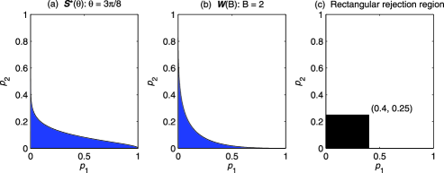
Figure 1: Compare shapes of rejection regions $\mathbf{S}^{*}(\theta)$, $\mathbf{W}(B)$ and a rectangle. Here, the threshold $t=0.1$ is used in $\mathbf{S}^{*}(\theta)$ and $\mathbf{W}(B)$.

As a comparison, the shape of the rejection region $\mathbf{S}^{*}(\theta)$ is different from the rectangle used in the two-stage multiple testing procedure of Bourgonetal2010 ; see Figure 1. In addition, the philosophy underlying the two procedures varies. For the two-stage procedure, a multiple testing procedure is only applied to the subset of hypotheses survived from the filtering stage. In contrast, the proposed $\mathrm{SIM}$ procedure does not screen any hypotheses out, but projects the bivariate $p$-value into a single-index $p(\theta)$. After that, methods in Section 4 for estimation and control of $\mathrm{FDR}$ are implemented using all the $m$ hypotheses.

To draw connection to the weighted multiple testing procedure of Genoveseetal2006 , we first generate the weights from the preliminary $p$-values and then combine the primary $p$-values with the weights. To be specific, in the first stage, we generate cumulative weights Roederetal2006 proportional to $\{v_{i}=\Phi(\Phi^{-1}(1-p_{i1})-B)\dvtx i=1,\ldots,m\}$, where $B$ is a tuning parameter. Because the weights are constrained to have mean 1, $w_{i}=v_{i}/\bar{v}_{m}$ is a valid choice, where $\bar{v}_{m}=\sum_{i=1}^{m}\Phi(\Phi^{-1}(1-p_{i1})-B)/m$. In the second stage, standard $\mathrm{BH}$ procedure BenjaminiHochberg1995 is applied to the weighted $p$-values, that is, $\{{p_{i2}}/{w_{i}}\dvtx i=1,\ldots,m\}$. The rejection region of the weighted multiple testing procedure is formed by $\mathbf{W}(B)=\{\mathbf{p}\dvtx p_{2}\leq\frac{\Phi(\Phi^{-1}(1-p_{1})-B)}{\bar{v}_{m}}t\}$; see Figure 1 for the graphical illustration. Surprisingly, the $\mathrm{SIM}$ multiple testing procedure and the weighted multiple testing procedure share similar patterns of rejection.

4 Estimation and control of $\mathrm{FDR}$ for the $\mathrm{SIM}$ procedure

In this section, we will first investigate properties of the single-index $p(\theta)$, followed by utilizing these properties to estimate and control the false discovery rate. For each possible direction $\theta$, denote by $\{p_{i}(\theta)\dvtx i=1,\ldots,m\}$ the sequence of projected $p$-values. Let $F_{0}(t,\theta)$, $F_{1}(t,\theta)$ and $F(t,\theta)$ be the true null distribution, nonnull distribution and marginal distribution of $p(\theta)$, respectively. Similarly, $f_{0}(t,\theta)$, $f_{1}(t,\theta)$ and $f(t,\theta)$ are their corresponding density functions. Following notations in Section 2.1, the frequentist $\mathrm{FDR}$ and Bayesian $\mathrm{Fdr}$ for the projected $p$-values $\{p_{i}(\theta)\dvtx i=1,\ldots,m\}$ are defined by

$$\mathrm{FDR}(t,\theta) = E\biggl{\{}\frac{V(t,\theta)}{R(t,\theta)\vee 1}\biggr{\}},$$

$$\mathrm{Fdr}(t,\theta) = \frac{\pi_{0}F_{0}(t,\theta)}{F(t,\theta)},$$

respectively, where $V(t,\theta)=\#\{\mbox{true null }p_{i}(\theta)\dvtx p_{i}(\theta)\leq t\}$ and $R(t,\theta)=\break\#\{p_{i}(\theta)\dvtx p_{i}(\theta)\leq t\}$ are the number of hypotheses erroneously rejected and the number of hypotheses rejected, based on some significance rule for the sequence of projected $p$-values.

4.1 Property of the single-index $p(\theta)$

The true null distribution of $p(\theta)$ in (15) plays an important role in estimating the false discovery rate. From the theory of statistics, the theoretical true null distributions of $p_{1}$ and $p_{2}$ are uniform. In the special case where $p_{1}$ and $p_{2}$ are independent under the true null, it is straightforward to show that $p(\theta)$ under the true null also follows a uniform distribution. In general, the assumption (N1) with $\bolds{\mu}_{0}=\mathbf{0}$ facilitates us to derive the $\mathrm{CDF}$ of $p(\theta)$ under the true null hypothesis. To be specific,

$$F_{0}(t,\theta) = \mathrm{P}\bigl{(}p(\theta)\leq t|\mbox{true null}\bigr{)}=\Phi\biggl{(}\frac{\Phi^{-1}(t)}{\sigma_{0}(\theta)}\biggr{)},$$

where

$$\qquad\sigma_{0}(\theta)=\sqrt{\bigl{\{}\cos(\theta)\bigr{\}}^{2}\sigma_{0;1}^{2}+\bigl{\{}\sin(\theta)\bigr{\}}^{2}\sigma_{0;2}^{2}+2\rho_{0}\sigma_{0;1}\sigma_{0;2}\cos(\theta)\sin(\theta)},$$ (17)

and $\sigma_{0;1}$, $\sigma_{0;2}$ and $\rho_{0}$ are as defined in (11). The following two categories summarize some properties of $p(\theta)$. [(II)]

If $\sigma_{0}(\theta)=1$, $p(\theta)$ under the true null hypothesis follows a standard uniform distribution.

If $\sigma_{0}(\theta)\neq 1$, the true null distribution of $p(\theta)$ is not uniform but symmetric with respect to ${1}/{2}$.

If $p_{1}$ and $p_{2}$ are both uniformly distributed under the true null, the expression of $\sigma_{0}(\theta)$ can be further simplified to $\sqrt{1+\rho_{0}\sin(2\theta)}$. Under the independence assumption (i.e., $\rho_{0}=0$), $p(\theta)$ is uniform for all $\theta$, which belongs to category (I). The case of negative correlation (i.e., $\rho_{0}<0$) implies $\sigma_{0}(\theta)<1$, shrinking most of the projected points corresponding to the true null concentrating around the point $1/2$. Consequently, this case has better potential to be powerful. The positive correlation worsens the structure of $p$-values a little, shifting some of the combined $p$-values corresponding to the true null to the area adjacent to 0 or 1, but it is still symmetric with respect to $1/2$. ZhangFanYu2011 employed a $p^{*}$-value, the median of $p$-values in the neighborhood of the original $p$-value, to capture the geometric feature in brain imaging. The true null distribution of $p^{*}$ is beta, which is symmetric with respect to ${1}/{2}$. Thus, the pair $(p,p^{*})$ of $p$-values belongs to category (II).

Although the assumption (N1) is imposed when deriving the specific form of $F_{0}(t,\theta)$, we could relax the normality assumption by assuming that the true null distribution of $p(\theta)$ is symmetric about $1/2$ for all $\theta$. The symmetry property assumption can be equivalently stated as: [(N3)]

The probability density function of $\mathbf{p}$ under the true null is centrally symmetric with respect to the point $(1/2,1/2)$, that is, $f_{0}(p_{1},p_{2})=f_{0}(1-p_{1},1-p_{2})$. (N3) provides flexibility in accommodating a wider range of distributions for $\mathbf{p}$. For example, (N3) holds if the bivariate test statistic under the true null follows a bivariate $t$ distribution for one-sided hypotheses; see (B) in Appendix B. In addition to estimating the parameter $\sigma_{0}(\theta)$, Section 4.2 will develop an adaptive data-driven estimator for $F_{0}(t,\theta)$ using a nonparametric approach based on (N3). While this relaxed assumption causes certain loss in efficiency for estimating $F_{0}(t,\theta)$, it achieves a gain in robustness.

4.2 Estimating the true null distribution of $p(\theta)$

Recall the properties of $p(\theta)$ in Section 4.1. If the normality assumption (N1) holds, one can estimate the true null distribution of $p(\theta)$ using the following parametric approach:

$$\widehat{F}_{0}^{\mathrm{I}}(t,\theta)=\Phi\biggl{(}\frac{\Phi^{-1}(t)}{\hat{\sigma}_{0}(\theta)}\biggr{)},$$ (18)

where $\hat{\sigma}_{0}(\theta)$ stands for some parametric estimator of $\sigma_{0}(\theta)$. Here, we will provide a simple and efficient estimator in the following procedure: [(a)]

Select a constant $c\geq 0$, such that $z$-values, $z(\theta)=\Phi^{-1}(p(\theta))$, from $(-c,\infty]$ are more likely to come from the true null hypothesis.

Split the data $\{z_{i}(\theta)\dvtx i=1,\ldots,m\}$ into three parts, that is, $\widetilde{Z}_{[-\infty,-c]}$, $\widetilde{Z}_{(-c,c]}$, and $\widetilde{Z}_{(c,\infty]}$, where the notation $\widetilde{Z}_{I}$ denotes the sample from interval $I$. Here, $I$ can be a closed, open or half-open interval.

Drop the sample $\widetilde{Z}_{[-\infty,-c]}$ and impute $-\widetilde{Z}_{[c,\infty]}$ into the interval$[-\infty,-c]$. $\hat{\sigma}_{0}(\theta)$ is the standard error of the newly constructed data $\widetilde{Z}{}^{*}=\{-\widetilde{Z}_{[c,\infty)},\widetilde{Z}_{(-c,c]},\widetilde{Z}_{(c,\infty)}\}$.

If the normality assumption (N1) is violated, we provide a nonparametric estimator based on the assumption (N3). The nonparametric approach follows the idea of ZhangFanYu2011 . To be specific, $F_{0}(t,\theta)$ can be estimated by the empirical distribution function,

$$\widehat{F}_{0}^{\mathrm{II}}(t,\theta) = \cases{\displaystyle\frac{\sum_{i=1}^{m}\mathrm{I}\{p_{i}(\theta)\geq(1-t)\}}{2\sum_{i=1}^{m}\mathrm{I}\{p_{i}(\theta)>0.5\}+\sum_{i=1}^{m}\mathrm{I}\{p_{i}(\theta)=0.5\}},\vspace*{5pt}\cr\qquad\mbox{if $0\leq t\leq 0.5$},\vspace*{6pt}\cr\displaystyle 1-\frac{\sum_{i=1}^{m}\mathrm{I}\{p_{i}(\theta)\geq t\}}{2\sum_{i=1}^{m}\mathrm{I}\{p_{i}(\theta)>0.5\}+\sum_{i=1}^{m}\mathrm{I}\{p_{i}(\theta)=0.5\}},\vspace*{5pt}\cr\qquad\mbox{if $0.5<t\leq 1$.}}$$ (19)

4.3 Estimating the proportion $\pi_{0}$ of true null hypotheses

There is an active research pursued in estimating $\pi_{0}$ (e.g., BenjaminiHochberg2000 , Benjaminietal2006 , HochbergBenjamini1990 , LiangNettleton2012 , SchwederSpjtvoll1982 , Storey2002 , Storeyetal2004 ). Storey2002 and Storeyetal2004 proposed an estimator $\hat{\pi}_{0}(\lambda)=\{m-R(\lambda)\}/\{(1-\lambda)m\}$ with a tuning parameter $\lambda$ in $[0,1)$ to be specified. LiangNettleton2012 summarized many adaptive and dynamically adaptive procedures for estimating $\pi_{0}$ and proposed a unified dynamically adaptive procedure. In this paper, we follow the same principle in LiangNettleton2012 and propose two estimators of $\pi_{0}$ dynamically according to two estimators of the true null distribution of $p(\theta)$ proposed in (18) and (19), respectively,

$$\hat{\pi}{}^{\mathrm{I}}_{0}(\theta) = \frac{m-R(\hat{\lambda}{}^{\mathrm{I}}(\theta),\theta)}{\{1-\widehat{F}_{0}^{\mathrm{I}}(\hat{\lambda}{}^{\mathrm{I}}(\theta),\theta)\}m},$$

$$\hat{\pi}{}^{\mathrm{II}}_{0}(\theta) = \frac{m-R(\hat{\lambda}{}^{\mathrm{II}}(\theta),\theta)}{\{1-\widehat{F}_{0}^{\mathrm{II}}(\hat{\lambda}{}^{\mathrm{II}}(\theta),\theta)\}m},$$

where $\hat{\lambda}{}^{\mathrm{I}}(\theta)$ and $\hat{\lambda}{}^{\mathrm{II}}(\theta)$ are dynamically chosen as in the algorithm below. [(For choosing $\lambda$)] For a sequence of values $0\equiv\lambda_{0}<\lambda_{1}<\cdots<\lambda_{n}\leq 1/2$, $\hat{\lambda}(\theta)$ is chosen to be $\lambda_{I^{*}}$, where $I^{*}=\min\{1\leq j\leq n-1\dvtx\break\hat{\pi}_{0}(\lambda_{j},\theta)\geq\hat{\pi}_{0}(\lambda_{j-1},\theta)\}$ if $\hat{\pi}_{0}(\lambda_{j},\theta)\geq\hat{\pi}_{0}(\lambda_{j-1},\theta)$ for some $j=1,\ldots,n-1$ and $\lambda_{I^{*}}=\lambda_{n}$ otherwise. Here, $\hat{\pi}_{0}(\lambda,\theta)$ is defined as ${\sum_{i=1}^{m}\mathrm{I}\{p_{i}(\theta)>\lambda\}}/\break{[\{1-\widehat{F}_{0}(\lambda,\theta)\}m]}$, where the estimator $\widehat{F}_{0}$ can be either (18) or (19) for the $\mathrm{CDF}$ of $p(\theta)$ under the true null hypothesis.

Remark 4.

We make the remarks concerning the algorithm.

• The range $(0,1/2]$ of the sequence of values $\{\lambda_{i}\dvtx i=1,\ldots,n\}$ is different from that in the right boundary procedure proposed by LiangNettleton2012 , where $\lambda$ can be loosely selected from $[0,1)$. We restrict the range to ${1}/{2}$ from two perspectives. On the one hand, it can be verified that $\hat{\pi}_{0}^{\mathrm{II}}(\lambda,\theta)$ is a constant for all $\lambda\geq 1/2$ and $\theta$. On the other hand, condition (C5) in Appendix A that $F_{1}(1/2,\theta)=1$ for all $\theta$, guaranteeing the consistency of $\widehat{F}^{\mathrm{II}}_{0}(t,\theta)$, enables us to search for $\lambda$ in a narrower range, which will be more efficient in practice.

• Theoretically, it is equivalent to get $\lambda(\theta)$ as $\lambda(\theta)=\inf_{0\leq t\leq{1}/{2}}\{t\dvtx F_{1}(t,\theta)=1\}$. If $t\leq\lambda(\theta)$, there is an upward-bias for estimating $\pi_{0}$, that is, $\pi_{1}\times\frac{1-F_{1}(t,\theta)}{1-F_{0}(t,\theta)}$; if $t>\lambda(\theta)$, the variance of $\hat{\pi}_{0}(t,\theta)$ is proportional to ${1}/[\{1-F_{0}(t,\theta)\}^{2}m]$. Instead of estimating $F_{1}(t,\theta)$, the algorithm described in the algorithm paragraph provides a rough but simple approach to estimate $\lambda(\theta)$. Here, we would like to point out that fixing $\lambda$ is not applicable to our approach, since $\lambda(\theta)$ varies with the tuning parameter $\theta$.

4.4 Selection of projection direction $\theta$

A specific $\theta$ corresponds to a projection direction, $(\cos(\theta),\sin(\theta))$ in (15), for the transformed $p$-value $(\Phi^{-1}(p_{1}),\Phi^{-1}(p_{2}))$. The choice of $\theta=0$ amounts to utilizing $p_{1}$ alone, whereas setting $\theta=\pi/2$ is equivalent to making inference with the information from $p_{2}$ alone. This indicates that our method indeed generalizes the conventional multiple testing. Recalling the shape of rejection region (16) and the criteria (8), different values of $\theta$ correspond to different shapes of rejection regions and the one with the highest power is preferred. Denote by $\theta_{0}(\alpha^{\prime})$ the optimal value of $\theta$, that is,

$$\theta_{0}\bigl{(}\alpha^{\prime}\bigr{)}=\arg\max_{0\leq\theta\leq\pi/2}F_{1}\bigl{(}t^{*}_{\alpha^{\prime}}(\theta),\theta\bigr{)},$$ (21)

where $t^{*}_{\alpha^{\prime}}(\theta)=\sup\{0\leq t\leq 1\dvtx{F_{0}(t,\theta)}/{F(t,\theta)}\leq\alpha^{\prime}\}$ and $0<\alpha^{\prime}<1$. The threshold $t^{*}_{\alpha^{\prime}}(\theta)$ in criteria (21) is chosen such that $\mathrm{Fdr}$ with respect to various $\theta$ is controlled at level $\pi_{0}\alpha^{\prime}$.

Proposition 2.

Suppose that $F_{0}(t,\theta)$ and $F_{1}(t,\theta)$ are continuously differentiable and $\frac{\partial F_{1}(t,\theta)}{\partial t}-\beta\frac{\partial F_{0}(t,\theta)}{\partial t}\neq 0$ with $\beta=(1/\alpha^{\prime}-\pi_{0})/\pi_{1}$, for any interior point $(t,\theta,\alpha^{\prime})$ in $[0,1]\times[0,\pi/2]\times[0,1/\pi_{0}]$. Then $\theta_{0}(\alpha^{\prime})$ in criteria (21) is constant for all $0<\alpha^{\prime}<1/\pi_{0}$, if and only if the solution $\theta$ of $t$ of the equation

$$\frac{\partial F_{1}(t,\theta)}{\partial t}\Big{/}\frac{\partial F_{1}(t,\theta)}{\partial\theta}=\frac{\partial F_{0}(t,\theta)}{\partial t}\Big{/}\frac{\partial F_{0}(t,\theta)}{\partial\theta}$$ (22)

is unique and equals a constant. Particularly, the above condition is satisfied under assumptions (N1) and (N2) with $\Sigma_{0}=\Sigma_{1}$.

Proposition 2 implies that $\theta_{0}(\alpha^{\prime})$ does not depend on $\alpha^{\prime}$ when $(\Phi^{-1}(p_{1}),\break\Phi^{-1}(p_{2}))$ is bivariate normally distributed with identical covariance matrix under the true null and nonnull. For bivariate normal models with unequal covariance matrices, Figure 2 shows that $\theta(\alpha^{\prime})$ varies slightly with $\alpha^{\prime}$. Numerical studies in Section 6 further confirm that $\theta_{0}(\alpha^{\prime})$ is robust to other bivariate distributions. Hence, the selection of $\alpha^{\prime}$ can be quite flexible except that only mild restriction needs to be imposed to make $\theta_{0}(\alpha^{\prime})$ identifiable based on conditions (C7) to (C10) in Appendix A. In particular, setting $\alpha^{\prime}=\alpha/\pi_{0}$ will ensure that the $\mathrm{Fdr}$ for various $\theta$ be controlled exactly at $\alpha$.

The Bayesian $\mathrm{Fdr}$ formula is equivalent to $F_{1}(t,\theta)=\frac{1-\pi_{0}\alpha^{\prime}}{1-\pi_{0}}F(t,\theta)$,implying that the criteria in (21) can be replaced by $\theta_{0}(\alpha^{\prime})=\break\arg\max_{0\leq\theta\leq\pi/2}F(t^{*}_{\alpha^{\prime}}(\theta),\theta)$. In Section 4.2, we have two types of estimators for $F_{0}(t,\theta)$, which can be used to develop estimation approach for $\theta$. Denoting $\widehat{F}_{0}(t,\theta)$ to be either type of estimator, the plug-in method for choosing the optimal direction $\theta_{0}(\alpha^{\prime})$ is thus given by

$$\hat{\theta}\bigl{(}\alpha^{\prime}\bigr{)}=\arg\max_{0\leq\theta\leq\pi/2}\frac{R(\hat{t}^{*}_{\alpha^{\prime}}(\theta),\theta)}{m},$$ (23)

where $\hat{t}^{*}_{\alpha^{\prime}}(\theta)=\sup\{0\leq t\leq 1\dvtx{m\widehat{F}_{0}(t,\theta)}/{\{R(t,\theta)\vee 1\}}\leq\alpha^{\prime}\}$. For notational clarity, we denote by $\{\hat{t}{}_{\alpha^{\prime}}^{*\mathrm{I}}(\theta),\hat{\theta}{}^{\mathrm{I}}(\alpha^{\prime})\}$ and $\{\hat{t}_{\alpha^{\prime}}^{*\mathrm{II}}(\theta),\hat{\theta}{}^{\mathrm{II}}(\alpha^{\prime})\}$ the estimators of $\{t^{*}_{\alpha^{\prime}}(\theta),\theta_{0}(\alpha^{\prime})\}$ obtained by the parametric and nonparametric approaches, respectively.

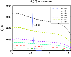
Figure 2: Illustrate the optimal projection direction $\theta_{0}(\alpha^{\prime})$ in (21) for various choices of $\alpha^{\prime}$ when $(\Phi^{-1}(p_{1}),\Phi^{-1}(p_{2}))$ follows (11) with ${\bolds{\mu}}_{0}=\mathbf{0}$, $\sigma_{0;1}=\sigma_{0;2}=1$, $\rho_{0}=0.2$ under the true null, and follows (12) with ${\bolds{\mu}}_{1}=(-2,-1.5)^{T}$, $\sigma_{1;1}=\sigma_{1;2}=1$, $\rho_{1}=0.6$ under nonnull, respectively. The solid line is the implicit curve $t=t(\theta)$ satisfying (22) in Proposition 2. From the proof of Proposition 2, the $x$-coordinates of the intersection points are $\theta_{0}(\alpha^{\prime})$.

4.5 Procedures for estimating and controlling $\mathrm{FDR}$

For each fixed $\theta$, we provide two methods for $\mathrm{FDR}$ estimation with respect to the projected $p$-values $\{p_{i}(\theta)\dvtx i=1,\ldots,m\}$ according to two estimators of $F_{0}(t,\theta)$ proposed in Section 4.2.

Incorporating the parametric approach for estimating $F_{0}(t,\theta)$ and $\pi_{0}$ leads to a procedure for estimation and control of $\mathrm{FDR}$. Combining (18) and (4.3), we propose

$$\widehat{\mathrm{FDR}}{}^{\mathrm{I}}(t,\theta)=\frac{\hat{\pi}_{0}^{\mathrm{I}}(\theta)\widehat{F}_{0}^{\mathrm{I}}(t,\theta)}{\{R(t,\theta)\vee 1\}/m}$$ (24)

for our $\mathrm{FDR}$ estimation. A conservative $\mathrm{FDR}$ estimator naturally leads to a procedure for controlling $\mathrm{FDR}$. Similar to (3), the data-driven threshold for the projected $p$-values $\{p_{i}(\theta)\dvtx i=1,\ldots,m\}$ is determined by

$$t_{\alpha}\bigl{(}\widehat{\mathrm{FDR}}{}^{\mathrm{I}}(:,\theta)\bigr{)}=\sup\bigl{\{}0\leq t\leq 1\dvtx\widehat{\mathrm{FDR}}{}^{\mathrm{I}}(t,\theta)\leq\alpha\bigr{\}}.$$ (25)

A null hypothesis is rejected if the corresponding $p(\theta)$ is less than or equal to the threshold $t_{\alpha}(\widehat{\mathrm{FDR}}{}^{\mathrm{I}}(:,\theta))$. The data-driven threshold (25) together with the point estimation method (24) for the false discovery rate comprises the first $\mathrm{FDR}$ procedure, denoted by $\mathrm{FDR}^{\mathrm{I}}$.

The nonparametric approach proposed for estimating $F_{0}(t,\theta)$ and $\pi_{0}$ can substitute the parametric counterpart in method I. Similar to (24) and (25), the procedure for the estimation and control of $\mathrm{FDR}$ is given by

$$\widehat{\mathrm{FDR}}{}^{\mathrm{II}}(t,\theta) = \frac{\hat{\pi}_{0}^{\mathrm{II}}(\theta)\widehat{F}_{0}^{\mathrm{II}}(t,\theta)}{\{R(t,\theta)\vee 1\}/m},$$ (26)

$$t_{\alpha}\bigl{(}\widehat{\mathrm{FDR}}{}^{\mathrm{II}}(:,\theta)\bigr{)} = \sup\bigl{\{}0\leq t\leq 1\dvtx\widehat{\mathrm{FDR}}{}^{\mathrm{II}}(t,\theta)\leq\alpha\bigr{\}}.$$ (27)

The second $\mathrm{FDR}$ procedure, denoted by $\mathrm{FDR}^{\mathrm{II}}$, consists of (26) and (27).

Remark 5.

Incorporating $\hat{\theta}{}^{\mathrm{I}}(\alpha^{\prime})$ and $\hat{\theta}{}^{\mathrm{II}}(\alpha^{\prime})$ obtained from Section 4.4 into $\mathrm{FDR}^{\mathrm{I}}$ and $\mathrm{FDR}^{\mathrm{II}}$, respectively, we obtain our final procedure for estimating and controlling $\mathrm{FDR}$.

4.6 Issue on stability and power for the $\mathrm{SIM}$ procedure

In this subsection, we first investigate the stability of the $\mathrm{SIM}$ procedure when the preliminary $p$-value is not accurate. Suppose that the bivariate $p$-value $(p_{1},p_{2})$ is calculated from the bivariate test statistic $(X_{1},X_{2})$ with marginal true null $\mathrm{CDF}$s $F_{0;X_{1}}$ and $F_{0;X_{2}}$. Due to some perturbation on $X_{1}$, we observe a contaminated version $\widetilde{X}_{1}$ with the true null $\mathrm{CDF}$ $F_{0;\widetilde{X}_{1}}$. By using the incorrect true null $\mathrm{CDF}$ $F_{0;X_{1}}$, the preliminary $p_{1}$ is incorrectly calculated as $\tilde{p}_{1}$. A natural question is how sensitive our $\mathrm{SIM}$ methods are if $X_{1}$ carries some wrong information.

Proposition 3.

Suppose $(X_{1},X_{2})$ are the preliminary and primary test statistics for one-sided hypotheses, where $F_{0;X_{1}}$ and $F_{0;X_{2}}$ are their marginal $\mathrm{CDF}$s under the true null, respectively. Assume the classical errors-in-variables model on $X_{1}$, that is, $\widetilde{X}_{1}=X_{1}+\eta$, where $\eta$ is independent of $(X_{1},X_{2})$ and the p.d.f.s of $X_{1}$ under the true null and $\eta$ are both symmetric with respect to $0$. If the joint p.d.f. of $(p_{1},p_{2})$ under the true null, where $(p_{1},p_{2})=(F_{0;X_{1}}(X_{1}),F_{0;X_{2}}(X_{2}))$ for left-sided hypotheses or $(p_{1},p_{2})=(1-F_{0;X_{1}}(X_{1}),\break 1-F_{0;X_{2}}(X_{2}))$ for right-sided hypotheses, is centrally symmetric with respect to $(1/2,1/2)$, then the joint p.d.f. of $(\tilde{p}_{1},p_{2})$ under the true null is also centrally symmetric with respect to $(1/2,1/2)$, where $\tilde{p}_{1}=F_{0;X_{1}}(\widetilde{X}_{1})$ for left-sided hypotheses or $\tilde{p}_{1}=1-F_{0;X_{1}}(\widetilde{X}_{1})$ for right-sided hypotheses.

Proposition 3 indicates that $\mathrm{FDR}$ of method $\mathrm{II}$ can still be controlled even if the preliminary test statistic is measured with classical additive error Carrolletal2010 . Although our discussion is restricted to the situation where the p.d.f. of preliminary test statistic under the true null is symmetric about 0, it indeed includes a large class of distributions, for example, normal distribution and $t$ distribution. In general, it can be verified that method $\mathrm{II}$ is valid if

$$f_{0;(\tilde{p}_{1},p_{2})}(\tilde{p}_{1},p_{2})\leq f_{0;(\tilde{p}_{1},p_{2})}(1-\tilde{p}_{1},1-p_{2}),$$ (28)

where $f_{0;(\tilde{p}_{1},p_{2})}(\tilde{p}_{1},p_{2})$ is the p.d.f. of $(\tilde{p}_{1},p_{2})$ under the true null and $\tilde{p}_{1}+p_{2}\leq 1$. Under (28), the probability mass under the true null in the upper-right tail of $(\tilde{p}_{1},p_{2})$ is no less than that in the lower-left tail, resulting in some conservative procedure. To simplify the argument, we only consider the case where $\tilde{p}_{1}$ and $p_{2}$ are independent, which simplifies the sufficient condition (28) to

$$f_{0;\tilde{p}_{1}}(\tilde{p}_{1})\leq f_{0;\tilde{p}_{1}}(1-\tilde{p}_{1}),$$ (29)

where $f_{0;\tilde{p}_{1}}(\tilde{p}_{1})$ is the p.d.f. of $\tilde{p}_{1}$ under the true null and $0\leq\tilde{p}_{1}\leq 1/2$. Some pairs of asymmetric distributions of ${X_{1}}$ and ${\widetilde{X}_{1}}$, satisfying the condition (29), are summarized below:

• ${X_{1}}\sim\operatorname{Exp}(\bar{\lambda}_{1})$ and ${\widetilde{X}_{1}}\sim\operatorname{Exp}(\bar{\lambda}_{2})$ with $\bar{\lambda}_{1}>\bar{\lambda}_{2}>0$, where $\operatorname{Exp}({\lambda})$ denotes the exponential distribution with parameter ${\lambda}$.

• ${X_{1}}\sim\chi^{2}_{r}$ and ${\widetilde{X}_{1}}\sim\chi^{2}_{s}$ with $r<s$.

• Chi-square versus weighted chi-square distribution
  ${X_{1}}\sim\chi^{2}_{r}$ and ${\widetilde{X}_{1}}\sim\sum_{i=1}^{r}\omega_{i}Z_{i}^{2}$, where $\{Z_{i}\}_{i=1}^{r}\stackrel{{\scriptstyle\mathrm{i.i.d.}}}{{\sim}}N(0,1)$ and $\omega_{i}\geq 1$, $i=1,\ldots,r$.

• $F$ versus generalized $F$ distribution
  ${X_{1}}\sim F(r,s)$ and ${\widetilde{X}_{1}}\sim\frac{(\sum_{i=1}^{r}\omega_{i}Z_{i}^{2})/r}{\chi^{2}_{s}/s}$, where $\{Z_{i}\}_{i=1}^{r}\stackrel{{\scriptstyle\mathrm{i.i.d.}}}{{\sim}}N(0,1)$, $\sum_{i=1}^{r}\omega_{i}Z_{i}^{2}$ is independent of $\chi^{2}_{s}$, and $\omega_{i}\geq 1$, $i=1,\ldots,r$.

Having established that the $\mathrm{SIM}$ procedure controls $\mathrm{FDR}$ when the preliminary $p$-values carry some wrong information, we next turn to theoretically justify why the current way of combination of the bivariate $p$-value achieves a higher power. Let $t_{\alpha}(\theta)$ denotes the threshold such that ${\pi_{0}F_{0}(t,\theta)}/\break{F(t,\theta)}=\alpha$. Then the power function can be formulated by $F_{1}(t_{\alpha}(\theta),\theta)=\beta^{\prime}F_{0}(t_{\alpha}(\theta),\theta)$, with $\beta^{\prime}=(1/\alpha-1)\pi_{0}/\pi_{1}$. Our goal is to quantify how much power can be improved via combining the bivariate $p$-value. From the Bayesian $\mathrm{Fdr}$ formula, the ratio of power of the $\mathrm{SIM}$ procedure to conventional multiple testing procedure using $p_{2}$ alone ($\theta=\pi/2$) can be derived as

$$\frac{F_{1}(t_{\alpha}(\theta),\theta)}{F_{1}(t_{\alpha}(\pi/2),\pi/2)} = \frac{F_{0}(t_{\alpha}(\theta),\theta)}{F_{0}(t_{\alpha}(\pi/2),\pi/2)}$$

$$= 1+\frac{({\partial}/({\partial\theta}))\{F_{0}(t_{\alpha}(\theta),\theta)\}|_{\theta={\pi/2}}(\theta-\pi/2)}{F_{0}(t_{\alpha}(\pi/2),\pi/2)}$$

$${}+O\bigl{(}(\theta-\pi/2)^{2}\bigr{)}$$

$$= 1+\Delta(\theta)+O\bigl{(}(\theta-\pi/2)^{2}\bigr{)}.$$

More derivations in Appendix B yield that the ratio of power improved when $\theta$ is close to $\pi/2$ is approximated by

$$1+\Delta(\theta) = 1+\frac{\phi[\Phi^{-1}\{t_{\alpha}(\pi/2)\}]f_{1;p_{2}}(t_{\alpha}(\pi/2))f_{0;p_{2}}(t_{\alpha}(\pi/2))}{f_{1;p_{2}}(t_{\alpha}(\pi/2))-\beta^{\prime}f_{0;p_{2}}(t_{\alpha}(\pi/2))}$$

$$\hskip 19.0pt\times\frac{(\theta-\pi/2)}{F_{0}(t_{\alpha}(\pi/2),\pi/2)}\times\mathrm{I}(p_{1}),$$

where $\mathrm{I}(p_{1})=E_{H_{0}}\{\Phi^{-1}(p_{1})|p_{2}=t_{\alpha}(\pi/2)\}-E_{H_{1}}\{\Phi^{-1}(p_{1})|p_{2}=t_{\alpha}(\pi/2)\}$, $f_{0;p_{2}}$ and $f_{1;p_{2}}$ are the p.d.f.s of $p_{2}$ under true null and nonnull, respectively. If the alternative distribution of $p_{2}$ is strictly concave, similar argument in GenoveseWasserman2002 yields that $f_{1;p_{2}}(t_{\alpha}(\pi/2))-\beta^{\prime}f_{0;p_{2}}(t_{\alpha}(\pi/2))<0$. The term $\mathrm{I}(p_{1})$ is positive, provided that the preliminary $p$-values have some potential to detect the power. Combining these, we have $1+\Delta(\theta)>1$.

Under assumptions (N1) and (N2), $\mathrm{I}(p_{1})$ has an explicit form

$$\bigl{[}\mu_{0;1}+\rho_{0}\sigma_{0;1}/\sigma_{0;2}\bigl{\{}\Phi^{-1}\bigl{(}t_{\alpha}(\pi/2)\bigr{)}-\mu_{0;2}\bigr{\}}\bigr{]}$$

(31)

$$\qquad{}-\bigl{[}\mu_{1;1}+\rho_{1}\sigma_{1;1}/\sigma_{1;2}\bigl{\{}\Phi^{-1}\bigl{(}t_{\alpha}(\pi/2)\bigr{)}-\mu_{1;2}\bigr{\}}\bigr{]}.$$

From (4.6), the correlation ($\rho_{0}$) between components of the bivariate $p$-value under the true null and that ($\rho_{1}$) under nonnull play different roles in improving power. The $\mathrm{SIM}$ procedure using prior information and primary $p$-values that are negatively correlated under the null hypothesis but positively correlated under the alternative is a general approach that can substantially increase power in practice.

5 Asymptotic justification

In many applications such as biology, medicine, genetics, neuroscience, economics and finance, tens of thousands of hypotheses are tested simultaneously. It is hence natural to investigate the behavior of the two approaches we proposed for the large number $m$ of hypotheses. In this section, we focus on the asymptotic properties of the nonparametric estimator, $\widehat{\mathrm{FDR}}{}^{\mathrm{II}}(t,\hat{\theta}{}^{\mathrm{II}}(\alpha^{\prime}))$. All theorems presented in this section can be derived similarly for the parametric approach as long as the bivariate normality for $(\Phi^{-1}(p_{1}),\Phi^{-1}(p_{2}))$ is satisfied.

Theorem 1 below establishes the consistency of $\hat{\theta}{}^{\mathrm{II}}(\alpha^{\prime})$. Intuitively, $\hat{\theta}{}^{\mathrm{II}}(\alpha^{\prime})$ is analogous to an $\mathrm{M}$-estimator such as least-squares estimators and many maximum-likelihood estimators. However, typical proof of consistency of $\mathrm{M}$-estimators is not applicable to $\hat{\theta}(\alpha^{\prime})$ because the $\mathrm{CDF}$ involved in (23) is not differentiable. Hence, the theoretical derivation is nontrivial and challenging. We will provide Lemmas 1–3 in Appendix A, which are necessary for proving Theorem 1.

Theorem 1

Assume conditions (C1) to (C9) in Appendix A. Then $\hat{\theta}{}^{\mathrm{II}}(\alpha^{\prime})$ converges to $\theta_{0}(\alpha^{\prime})$ almost surely.

Theorem 2 below reveals that the proposed estimator $\widehat{\mathrm{FDR}}{}^{\mathrm{II}}$ not only controls the $\mathrm{FDR}$ simultaneously for all $t\geq\delta$ and $\delta>0$ for fixed $\theta$, but also provides simultaneous and conservative control when incorporating the data-driven estimator $\hat{\theta}{}^{\mathrm{II}}(\alpha^{\prime})$.

Theorem 2

Assume conditions (C1) to (C10) in Appendix A. Then $\widehat{\mathrm{FDR}}{}^{\mathrm{II}}(t,\hat{\theta}{}^{\mathrm{II}}(\alpha^{\prime}))$ provides simultaneously conservative control of $\mathrm{FDR}(t,\break\theta_{0}(\alpha^{\prime}))$ in the sense that

$$\lim_{m\to\infty}\inf_{t\geq\delta}\bigl{\{}\widehat{\mathrm{FDR}}{}^{\mathrm{II}}\bigl{(}t,\hat{\theta}{}^{\mathrm{II}}\bigl{(}\alpha^{\prime}\bigr{)}\bigr{)}-\mathrm{FDR}\bigl{(}t,\theta_{0}\bigl{(}\alpha^{\prime}\bigr{)}\bigr{)}\bigr{\}} \geq 0,$$

$$\lim_{m\to\infty}\inf_{t\geq\delta}\biggl{\{}\widehat{\mathrm{FDR}}{}^{\mathrm{II}}\bigl{(}t,\hat{\theta}{}^{\mathrm{II}}\bigl{(}\alpha^{\prime}\bigr{)}\bigr{)}-\frac{V(t,\theta_{0}(\alpha^{\prime}))}{R(t,\theta_{0}(\alpha^{\prime}))\vee 1}\biggr{\}} \geq 0$$

with probability $1$.

To show that the proposed estimator $\widehat{\mathrm{FDR}}{}^{\mathrm{II}}(t,\hat{\theta}{}^{\mathrm{II}}(\alpha^{\prime}))$ provides strong control of $\mathrm{FDR}(t,\theta_{0}(\alpha^{\prime}))$ asymptotically, we define

$$\widehat{\mathrm{FDR}}_{\lambda}^{\infty}(t,\theta)=\frac{\{\pi_{0}+\pi_{1}(({1-F_{1}(\lambda,\theta)})/({1-F_{0}(\lambda,\theta)}))\}F_{0}(t,\theta)}{F(t,\theta)},$$

which is a pointwise limit of $\widehat{\mathrm{FDR}}_{\lambda}^{\mathrm{II}}(t,\theta)=\frac{\hat{\pi}_{0}^{\mathrm{II}}(\lambda,\theta)\widehat{F}_{0}^{\mathrm{II}}(t,\theta)}{\{R(t,\theta)\vee 1\}/m}$ under conditions (C1) and (C2) and Lemma 2 in Appendix A. The notations $\hat{\pi}_{0}^{\mathrm{I}}(\lambda,\theta)$ and $\hat{\pi}_{0}^{\mathrm{II}}(\lambda,\theta)$ are defined in a way similar to those in the algorithm of Section 4.3.

Theorem 3

Assume conditions (C1) to (C10) in Appendix A. Also, suppose that the sequence of values $\{\lambda_{j}\dvtx j=1,\ldots,n\}\in(0,1/2]^{n}$ and $n$ is a fixed finite integer. If for each $\lambda_{j}$, there is $t_{j}\in(0,1]$ such that $\widehat{\mathrm{FDR}}{}^{\infty}_{\lambda_{j}}(t_{j},\break\theta_{0}(\alpha^{\prime}))<\alpha$, then

$$\limsup_{m\to\infty}\mathrm{FDR}\bigl{(}t_{\alpha^{\prime}}\bigl{(}\widehat{\mathrm{FDR}}{}^{\mathrm{II}}\bigl{(}:,\hat{\theta}{}^{\mathrm{II}}\bigl{(}\alpha^{\prime}\bigr{)}\bigr{)}\bigr{)},\hat{\theta}{}^{\mathrm{II}}\bigl{(}\alpha^{\prime}\bigr{)}\bigr{)}\leq\alpha.$$

6 Numerical studies

In this section, we carry out simulation studies to evaluate the performance of the $\mathrm{SIM}$ procedure in the aspects of controlling $\mathrm{FDR}$ and detection power, using the two proposed methods under various bivariate models for the preliminary and primary test statistics. The sequence of values $\{\lambda_{j}\dvtx j=1,\ldots,n\}$ in the algorithm of Section 19 is $\{0.02,0.04,0.06,0.08,0.1,0.125,0.15,\ldots,0.5\}$. For simplicity, the constant $c$ in Section 4.2 is set to be 0. Unless otherwise stated, $\alpha^{\prime}$ is simply set to be $\alpha$ throughout this section, following Proposition 2. All simulations are based on $500$ replications.

The following procedures are compared:

• Conventional $\mathrm{FDR}$ procedure: the $\mathrm{FDR}$ method using (2) and (3) with $\pi_{0}$ dynamically selected by the algorithm in Section 4.3.

• Weighted multiple testing procedure: the weighted multiple testing procedure proposed by Genoveseetal2006 , where the weighting scheme is determined automatically by the preliminary $p$-values; refer to the cumulative weights with $B=2$ in Section 3.3 for detail.

• Two-stage multiple testing procedure: the two-stage procedure defined by Bourgonetal2010 with the first stage being preliminary $p$-values filtering. The proportion of hypotheses to be removed in the filtering stage is set to be 50%.

Note that the “50% variance filter” in Bourgonetal2010 shares the same spirit as the “two-stage multiple testing procedure” except that the overall sample variance serves as the filter statistic.

6.1 Example 1: Bivariate normal model

This example comes from hypothesis testing of mean shift in normal models, that is, $X=\mu+\varepsilon$ with $\varepsilon\sim N(0,1)$. We perform $m={}$10,000 independent right-sided hypotheses testing for $H_{0}\dvtx\mu=0$ versus $H_{1}\dvtx\mu>0$. Among all the null hypotheses, a proportion $\pi_{0}$ of them are from the true null hypotheses. For the $i$th test, we generate a bivariate test statistic $(x_{i1},x_{i2})$ from a bivariate normal distribution $\mathcal{N}(\bolds{\mu},\Sigma)$ where $\Sigma=(\sigma_{ij})_{2\times 2}$ with $\sigma_{11}=1$, $\sigma_{12}=\sigma_{21}=\rho$ and $\sigma_{22}=1$. We set $\bolds{\mu}=\mathbf{0}$ under the true null and $\bolds{\mu}=(\mu_{1},\mu_{2})$ under nonnull. The marginal $p$-values for the $i$th test are $p_{i1}=1-\Phi(x_{i1})$ and $p_{i2}=1-\Phi(x_{i2})$, for $i=1,\ldots,m$.

To evaluate the overall performance of the estimated $\mathrm{FDR}(t,\theta)$ of methods I and II at the same threshold $t\in[0,1]$, we consider the scenario where $\mu_{1}=\mu_{2}=2$, $\pi_{0}=0.75$ and $\rho=0.2$. For notational convenience, denote by $\mathrm{FDP}(t,\theta)=V(t,\theta)/\{R(t,\theta)\vee 1\}$ the false discovery proportion at threshold $t$ with respect to $\{p_{i}(\theta)\dvtx i=1,\ldots,m\}$. Figure 3 compares the average values of $\widehat{\mathrm{FDR}}{}^{\mathrm{I}}(t,\theta)$, $\widehat{\mathrm{FDR}}{}^{\mathrm{II}}(t,\theta)$ and $\mathrm{FDP}(t,\theta)$ for $\theta=\pi/8$, $\pi/4$, $3\pi/8$. For each case, these two types of estimators are very close to true $\mathrm{FDP}$, lending support to the parametric and nonparametric estimation procedures in Section 4.

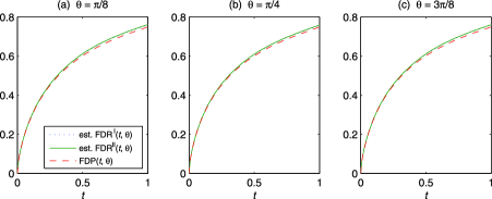
Figure 3: Estimated $\mathrm{FDR}$ for methods $\mathrm{I}$ and $\mathrm{II}$ and the corresponding true $\mathrm{FDP}$ as a function of threshold $t$ and $\theta$ in Example $1$. Here, $\mu_{1}=\mu_{2}=2$, $\pi_{0}=0.75$ and $\rho=0.2$.

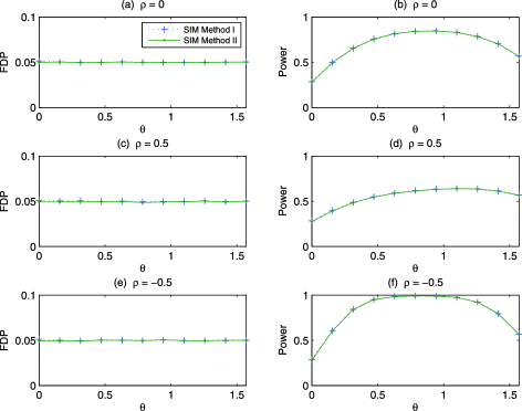
Figure 4: Calculated $\mathrm{FDP}$ and power as a function of $\theta$ and $\rho$ in Example $1$. Here, $\mu_{1}=2$, $\mu_{2}=2.5$, $\pi_{0}=0.75$ and $\alpha=0.05$.

To illustrate the role of $\theta$ for detecting power in our proposed procedure, a sequence of values $\{\theta_{l}=(l-1)/10\times\pi/2\dvtx l=1,\ldots,11\}$ are designed. For simplicity, we consider the scenario where $\mu_{1}=2,\mu_{2}=2.5$, $\pi_{0}=0.75$, $\alpha=0.05$ and $\rho=\{0,0.5,-0.5\}$. Figure 4 corresponds to the calculated $\mathrm{FDP}$ [i.e., $\mathrm{FDP}(\hat{t}_{\alpha})$] and the calculated power [i.e., $S(\hat{t}_{\alpha})/m_{1}$] as a function of $\theta$, for $\rho=0,0.5,-0.5$, respectively. In either case, we observe that the average values of the calculated $\mathrm{FDP}$ for both $\mathrm{FDR}^{\mathrm{I}}$ and $\mathrm{FDR}^{\mathrm{II}}$ are almost controlled at $\alpha=0.05$ for all $\theta$, and by appropriately choosing $\theta$, the $\mathrm{SIM}$ methods outperform the conventional $\mathrm{FDR}$ procedure using $p_{2}$ alone (with $\theta=\pi/2$). The correlation between the components of the bivariate $p$-value sensitively affects the optimal power. Negative correlation distinguishes $p_{1}$ and $p_{2}$ most significantly, thus it is expected that this case can improve the power most via combining the bivariate $p$-value. As a comparison, positive correlation diminishes the detection slightly. However, the power is still improved significantly when comparing to the conventional $\mathrm{FDR}$ procedure using $p_{2}$ alone.

To confirm the consistency of $\hat{\theta}(\alpha^{\prime})$, we compare 10 scenarios, where $\pi_{0}=0.75$, $\rho=0.2$, $\alpha^{\prime}=\{0.05,0.1\}$ and $(\mu_{1},\mu_{2})$ takes five different pair-values. From Proposition 2, the optimal value $\theta_{0}(\alpha^{\prime})$ is constant for different $\alpha^{\prime}$, denoted by $\theta_{0}$. Table 2 compares the average value of $\hat{\theta}(\alpha^{\prime})$ and its standard error of methods I and II with the optimal value $\theta_{0}$. In all situations, estimators are very close to the optimal value $\theta_{0}$ except that the standard error of $\hat{\theta}(\alpha^{\prime})$ by method II is slightly larger than that by method I. This phenomenon is not surprising, since the nonparametric fit for $F_{0}(t,\theta)$ and $F(t,\theta)$ contaminates the estimator $\hat{\theta}{}^{\mathrm{II}}(\alpha^{\prime})$. For unequal covariance matrices in bivariate normal models for $(x_{i1},x_{i2})$ with the correlation coefficients $\rho_{0}$ and $\rho_{1}$ in the true null and nonnull, respectively, Figure 5 shows the stability of $\hat{\theta}(\alpha^{\prime})$ for various choices of $\alpha^{\prime}$ using both methods I and II.

Table 2: Mean and standard error of $\hat{\theta}(\alpha^{\prime})$ by $\mathrm{FDR}^{\mathrm{I}}$ and $\mathrm{FDR}^{\mathrm{II}}$ for $10$ scenarios, where $\pi_{0}=0.75$, $\rho=0.2$, $\alpha^{\prime}=\{0.05,0.10\}$ and $(\mu_{1},\mu_{2})$ are set to be $(2,1)$, $(2,1.5)$, $(2,2)$, $(2,2.5)$, $(2,3)$, respectively

	$\bolds{\alpha^{\prime}=0.05}$		$\bolds{\alpha^{\prime}=0.10}$
$\bolds{(\mu_{1},\mu_{2})}$	$\bolds{\mathrm{FDR}^{\mathrm{I}}}$	$\bolds{\mathrm{FDR}^{\mathrm{II}}}$	$\bolds{\mathrm{FDR}^{\mathrm{I}}}$	$\bolds{\mathrm{FDR}^{\mathrm{II}}}$	$\bolds{\theta_{0}}$
(2, 1)	0.3231 (0.07)	0.3273 (0.13)	0.3190 (0.07)	0.3192 (0.10)	0.3218
(2, 1.5)	0.5706 (0.07)	0.5713 (0.12)	0.5684 (0.07)	0.5687 (0.10)	0.5743
(2, 2)	0.7785 (0.06)	0.7828 (0.11)	0.7813 (0.07)	0.7808 (0.09)	0.7854
(2, 2.5)	0.9523 (0.06)	0.9525 (0.09)	0.9436 (0.07)	0.9490 (0.09)	0.9505
(2, 3)	1.0732 (0.06)	1.0734 (0.09)	1.0720 (0.08)	1.0755 (0.11)	1.0769

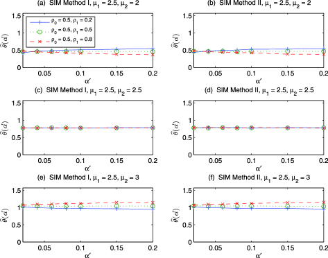
Figure 5: $\hat{\theta}(\alpha^{\prime})$ as a function of $\alpha^{\prime}$ for various combination of $(\mu_{1},\mu_{2},\rho_{0},\rho_{1})$ in bivariate normal models for $(x_{i1},x_{i2})$. Here, $\pi_{0}=0.75$.

In the previous simulation results, we have demonstrated that for a fixed value of $\theta$, $\widehat{\mathrm{FDR}}{}^{\mathrm{I}}$ and $\widehat{\mathrm{FDR}}{}^{\mathrm{II}}$ provide simultaneous and conservative control of $\mathrm{FDR}$; and that power can improve significantly by appropriately choosing $\theta$. Does the conclusion continue to hold for random $\hat{\theta}(\alpha)$? Figure 6 examines the control of $\mathrm{FDR}$ as well as power comparison of the $\mathrm{SIM}$ methods, their corresponding contaminated versions and the conventional $\mathrm{FDR}$ procedure for various combinations of $(\mu_{2},\pi_{0})$. The left panels of Figure 6 compare the calculated $\mathrm{FDP}$ of all settings. Clearly, the calculated $\mathrm{FDP}$ for the $\mathrm{SIM}$ methods and their contaminated versions is controlled at the prespecified $\alpha=0.05$, confirming that the $\mathrm{SIM}$ methods are still valid when the preliminary test statistics carry some wrong information. The right panels correspond to the power of all the approaches. We observe that the average values of power of $\mathrm{FDR}^{{\mathrm{I}}}(t,\hat{\theta}(\alpha))$ and $\mathrm{FDR}^{{\mathrm{II}}}(t,\hat{\theta}(\alpha))$ are consistently higher than that of the conventional $\mathrm{FDR}$ procedure using $p_{2}$ alone. Remarkably, the power of the contaminated versions of the $\mathrm{SIM}$ methods is not adversely affected, but between that of the $\mathrm{SIM}$ methods and the conventional $\mathrm{FDR}$ procedure.

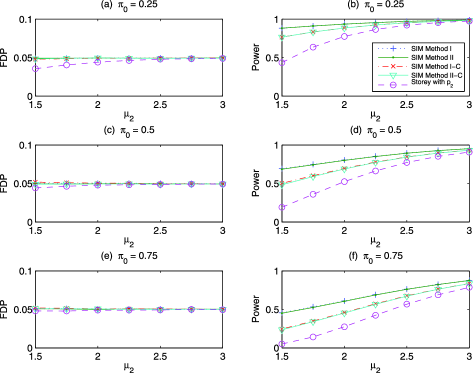
Figure 6: Calculated $\mathrm{FDP}$ and power as a function of $\mu_{2}$ and $\pi_{0}$ for the $\mathrm{SIM}$ methods, their contaminated versions $(\mathrm{SIM}$ method $\mathrm{I}$-C, $\mathrm{SIM}$ method $\mathrm{II}$-C) and the conventional $\mathrm{FDR}$ procedure (storey with $p_{2})$ in Example $1$. The contamination scheme is $\widetilde{X}_{1}=X_{1}+\eta$, where $\widetilde{X}_{1}$ is the observable preliminary test statistic and $\eta$ is a standard normal noise independent of the unobservable one $X_{1}$. Here, $\mu_{1}=2$, $\alpha=0.05$ and $\rho=0.2$.

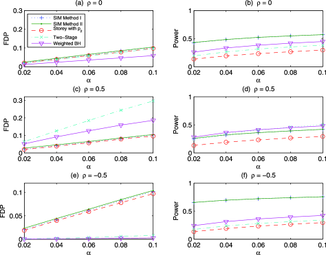
Figure 7: Calculated $\mathrm{FDP}$ and power as a function of $\alpha$ and $\rho$ for the $\mathrm{SIM}$ methods, the weighed multiple testing procedure (weighted $\mathrm{BH})$, the two-stage multiple testing procedure (two-stage) and the conventional $\mathrm{FDR}$ procedure (storey with $p_{2})$ in Example $1$. Here, the nonnull is a mixture of three bivariate normal distributions with signals $(1,1)$, $(2,2)$ and $(3,3)$, respectively, and $\pi_{0}=0.9$.

To further illustrate the advantage of the $\mathrm{SIM}$ methods, Figure 7 compares them with the weighted multiple testing procedure and the two-stage multiple testing procedure which virtually use the same amount of information from preliminary $p$-values and primary $p$-values for various levels $\alpha$ and $\rho$ when the nonnull is a mixture of three bivariate normal distributions with small, moderate and strong signals. When the preliminary $p$-value and primary $p$-value are independent, all the approaches are valid but the $\mathrm{SIM}$ methods outperform the weighted multiple testing procedure and the two-stage multiple testing procedure for all significant levels $\alpha$. Note that both the weighted multiple testing procedure and the two-stage multiple testing procedure are out of control if the components of bivariate $p$-value are positively correlated and much more conservative under negative dependence. In contrast, the $\mathrm{SIM}$ methods consistently estimate the $\mathrm{FDR}$ under any dependence structure between the components of bivariate $p$-value, providing much flexibility to choose filters or weights in practice.

6.2 Example 2: Bivariate $t$ distribution

In this example, we consider a set-up similar to Example 1 except that the datasets are generated from a bivariate $t$ distribution. To be specific, $\{(x_{i1},x_{i2})\dvtx i=1,\ldots,m\}$, are sampled independently from a bivariate $t$ distribution with $3$ degrees of freedom and covariance matrix identical to that in Example 1. Among all the null hypotheses, a proportion $\pi_{0}$ of them come from the true null hypotheses with mean zero, while the rest are coming from nonnull hypotheses with mean vector ${\bolds{\mu}}=(\mu_{1},\mu_{2})$.

Figure 8 compares the average values of the true $\mathrm{FDP}$, $\widehat{\mathrm{FDR}}{}^{\mathrm{I}}(t,\theta)$ and $\widehat{\mathrm{FDR}}{}^{\mathrm{II}}(t,\theta)$ in a zoomed-in region of $t\in[0,0.05]$ for different combinations of $(\pi_{0},\theta)$. On the right panels where $\theta=\pi/2$ (using $p_{2}$), both methods I and II provide conservative estimates of $\mathrm{FDR}$. For the case $\theta=\pi/4$ on the left panels, method II provides conservative estimation of $\mathrm{FDR}$ and is less conservative as $\pi_{0}$ increases. Unlike method $\mathrm{II}$, method $\mathrm{I}$ underestimates the true $\mathrm{FDR}$ for small $t$ and overestimates it for large $t$, which makes the $\mathrm{FDR}$ out of control for small $\alpha$. This is not surprising, since the bivariate $t$ distribution with very low degrees of freedom violates the normality assumption.

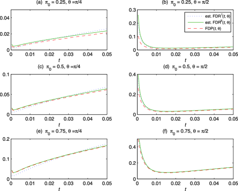
Figure 8: Estimated $\mathrm{FDR}$ for methods $\mathrm{I}$ and $\mathrm{II}$ and the corresponding true $\mathrm{FDP}$ as a function of $t$ in Example $2$. Here, $\mu_{1}=\mu_{2}=4$ and $\rho=0.2$.

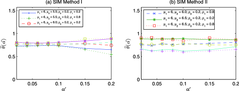
Figure 9: $\hat{\theta}(\alpha^{\prime})$ versus $\alpha^{\prime}$ for various combination of $(\mu_{1},\mu_{2},\rho_{0},\rho_{1})$ for bivariate $t$ distributions. Here, $\pi_{0}=0.75$.

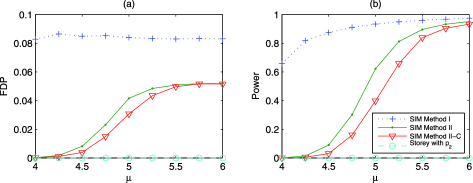
Figure 10: Calculated $\mathrm{FDP}$ and power as a function of $\mu$ $(\mu=\mu_{1}=\mu_{2})$ for the $\mathrm{SIM}$ methods, the contaminated version of method $\mathrm{II}$ $(\mathrm{SIM}$ method $\mathrm{II}$-C) and the conventional $\mathrm{FDR}$ procedure (storey with $p_{2})$ in Example $2$. The contamination scheme is $\widetilde{X}_{1}=X_{1}+\eta$, where $\widetilde{X}_{1}$ is the observable preliminary test statistic and $\eta$ is a standard normal noise independent of the unobservable one $X_{1}$ in Example $2$. Here, $\alpha=0.05$, $\rho=0.2$, $\pi_{0}=0.9$ and $\mathrm{df}=3$.

Before assessing the performance of the $\mathrm{SIM}$ methods incorporating random $\hat{\theta}(\alpha)$, we first demonstrate that $\hat{\theta}(\alpha^{\prime})$ is robust to $\alpha^{\prime}$ for various bivariate $t$ distributions in Figure 9, which lends support to setting $\alpha^{\prime}=\alpha$ when choosing the optimal projection direction. Based on this setting, Figure 10 summarizes the average values of the calculated $\mathrm{FDP}$ and power of the $\mathrm{SIM}$ methods, the contaminated version of method $\mathrm{II}$ and the conventional $\mathrm{FDR}$ procedure for various combinations of $(\mu_{1},\mu_{2})$. We observe that the conventional $\mathrm{FDR}$ procedure lacks the ability to detect statistical significance for various signals even when $\alpha=0.05$. Nonetheless, by incorporating the prior information from $p_{1}$ into $p_{2}$, method $\mathrm{II}$ improves the power while controlling the $\mathrm{FDR}$. Similar to the previous case (Figure 6), the calculated $\mathrm{FDP}$ for the contaminated version of method $\mathrm{II}$ is controlled at $\alpha=0.05$ and the corresponding power is very close to that of method $\mathrm{II}$. This illustrates the stability of method $\mathrm{II}$ when the preliminary $p$-value is not accurate. Note that, even if method $\mathrm{I}$ appears more powerful than method $\mathrm{II}$, the calculated $\mathrm{FDP}$ for method $\mathrm{I}$ is out of control at level higher than $\alpha=0.05$. The uncontrolled performance of method I indicates that the nonparametric approach has certain advantage in accommodating a larger class of bivariate distributions, and hence is practically more applicable.

Under a mixture of three bivariate $t$ distributions on the nonnull, the comparison of the $\mathrm{SIM}$ methods with the weighted multiple testing procedure and the two-stage multiple testing procedure is demonstrated in Figure 11. The story of bivariate $t$ distributions is similar to that of bivariate normal models in Figure 7 except that method $\mathrm{I}$ loses its validity for controlling $\mathrm{FDR}$ in all settings. In summary, method $\mathrm{II}$ has the merit of correctly and efficiently incorporating the prior information, such as filters in the two-stage multiple testing procedure and weights in the weighted multiple testing procedure, into the conventional $\mathrm{FDR}$ procedure under any dependence structure ($\rho$).

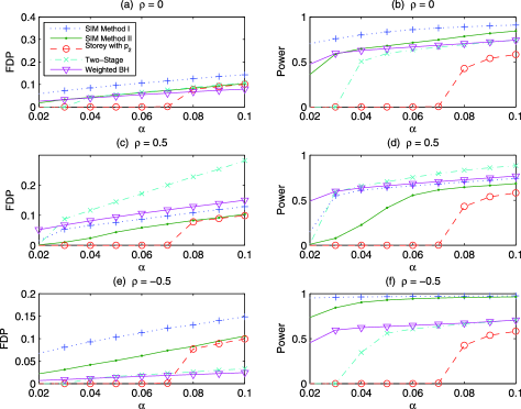
Figure 11: Calculated $\mathrm{FDP}$ and power as a function of $\alpha$ and $\rho$ for the $\mathrm{SIM}$ methods, the weighed multiple testing procedure (weight $\mathrm{BH})$, the two-stage multiple testing procedure (two-stage) and the conventional $\mathrm{FDR}$ procedure (storey with $p_{2})$ in Example $2$. Here, the nonnull is a mixture of three bivariate $t$ distributions with signals $(3,3)$, $(6,6)$ and $(8,8)$, respectively, and $\pi_{0}=0.9$.

6.3 Example 3: Multiple testing with serially clustered signals

In practice, nonnull hypotheses are typically clustered. Thus, we can take a preliminary $p$-value $p_{i1}$ to be the local aggregation of $p_{j2}$, for $j$ located in the neighborhood of the $i$th hypothesis, where $\{p_{i2}\dvtx i=1,\ldots,m\}$ are the primary $p$-values. The new pairs $\{(p_{i1},p_{i2})\dvtx i=1,\ldots,m\}$ consist of the bivariate $p$-values. In this example, we mimic the situation of serially clustered signals to evaluate the performance of the $\mathrm{SIM}$ methods. To be specific, we perform $m={}$10,000 one-sided hypotheses testing independently, where test statistics follow $N(0,1)$ and $N(\mu,1)$ for the true null and nonnull, respectively, for $\mu$ randomly chosen from $\{1.5,2,2.5\}$. The serial structure is designed as follows: the nonnull hypotheses consist of three clusters, that is, $\mathcal{C}_{1}=\{i=1001,\ldots,2000\},\mathcal{C}_{2}=\{i=5001,\ldots,6000\}$ and $\mathcal{C}_{3}=\{i=8001,\ldots,9000\}$. There are various types of preliminary $p$-values we can take, such as the mean or median of the $p$-values in the neighborhood of the original hypothesis; refer to ZhangFanYu2011 for details. For simplicity, the $p$-values in the neighborhood of $p_{i2}$ is chosen as $\{p_{i-1,2},p_{i+1,2}\}$ and the preliminary $p$-value is defined as $p_{i1}=({p_{i-1,2}+p_{i+1,2}})/{2}$, for $i=1,\ldots,m$. Besides the conventional $\mathrm{FDR}$ procedure, the mean filter, $p_{i}^{*}=({p_{i-1,2}+p_{i,2}+p_{i+1,2}})/{3}$ proposed by ZhangFanYu2011 , also serves as a competitor. The results are shown in Table 3. Method II, the mean filter using $p_{i}^{*}$ and the conventional $\mathrm{FDR}$ procedure using $p_{2}$ provide conservative control of $\mathrm{FDR}$, whereas $\mathrm{FDR}$ of method I is slightly out of control for small $\alpha$. This is reasonable as the normality assumption is not strictly satisfied for the transformed $p$-value $(\Phi^{-1}(p_{i1}),\Phi^{-1}(p_{i2}))$. In general, by utilizing the structural information of the primary $p$-values, both method II and the mean filter using $p_{i}^{*}$ are more powerful than the conventional $\mathrm{FDR}$ procedure using $p_{2}$ alone. Rather than giving the same weight $(1/3)$ to the neighborhood $(p_{i-1,2},p_{i,2},p_{i+1,2})$ in the mean filter $p_{i}^{*}$, the data-driven procedure for selecting $\theta$ based on power comparison for method II adjusts different weights to the bivariate $p$-value $(p_{i1},p_{i2})$ according to their corresponding potential for detecting power. Consequently, method II outperforms the mean filter using $p_{i}^{*}$ for all possible $\alpha$.

Table 3: Calculated $\mathrm{FDP}$ and power comparison of methods $\mathrm{I}$ and $\mathrm{II}$, the mean filter using $p_{i}^{*}$ and the conventional $\mathrm{FDR}$ procedure (storey with $p_{2})$ in Example $3$

	$\bolds{\mathrm{FDR}^{\mathrm{I}}}$ using $\bolds{(p_{1},p_{2})}$		$\bolds{\mathrm{FDR}^{\mathrm{II}}}$ using $\bolds{(p_{1},p_{2})}$		Mean filter using $\bolds{p_{i}^{*}}$		Storey with $\bolds{p_{2}}$
$\bolds{\alpha}$	$\bolds{\mathrm{FDP}}$	Power	$\bolds{\mathrm{FDP}}$	Power	$\bolds{\mathrm{FDP}}$	Power	$\bolds{\mathrm{FDP}}$	Power
0.01	0.013	0.617	0.010	0.578	0.010	0.505	0.010	0.059
0.02	0.024	0.708	0.020	0.684	0.020	0.616	0.019	0.115
0.03	0.034	0.759	0.030	0.742	0.030	0.682	0.029	0.164
0.04	0.044	0.794	0.040	0.782	0.040	0.728	0.038	0.208
0.05	0.053	0.820	0.050	0.811	0.050	0.763	0.048	0.247
0.06	0.063	0.841	0.060	0.834	0.060	0.791	0.058	0.283
0.07	0.073	0.858	0.070	0.852	0.070	0.813	0.067	0.317
0.08	0.082	0.872	0.079	0.867	0.080	0.832	0.077	0.348
0.09	0.092	0.884	0.089	0.881	0.090	0.849	0.087	0.377
0.10	0.101	0.894	0.099	0.891	0.100	0.864	0.096	0.404
0.20	0.196	0.952	0.199	0.953	0.199	0.945	0.192	0.610
0.30	0.293	0.977	0.299	0.978	0.299	0.978	0.288	0.748

6.4 Example 4: Two-sample $t$ test

In this example, we mimic the microarray experiment, where two-sample $t$ test is performed to detect differentially expressed genes for two classes comparison. Suppose $m={}$10,000 genes are examined independently, among which $10\%$ are from the nonnull. For the $i$th gene, let $\{x_{i,1},x_{i,2},\ldots,x_{i,10}\}$ and $\{y_{i,1},y_{i,2},\ldots,y_{i,10}\}$ be two independent samples from $N(\mu_{1},1)$ and $N(\mu_{2},1)$, respectively, where $\mu_{1}=\mu_{2}$ is for nondifferentially expressed genes and $\mu_{1}\neq\mu_{2}$ is for differentially expressed genes. The primary $p$-value, $p_{i2}$, is obtained by the standard two-sample $t$ test. To get the preliminary $p$-value, $p_{i1}$, the sum of squared error of the two samples, which has a chi-square distribution with $19$ degrees of freedom and independent of $t$ statistic in the standard two-sample $t$ test under the true null, can be utilized. In this scenario, the independence between the components of bivariate $p$-value implies that the true null distribution of the combined $p$-value is uniform for all $\theta$. To make a comprehensive comparison, the $50\%$ variance filter proposed in Bourgonetal2010 is also considered. Figure 12 shows that the performance of methods I and II is almost the same and the corresponding power is improved for different size effect $\mu_{1}-\mu_{2}$ for $\alpha=0.05$. Particularly, our method is superior to the $50\%$ variance filter for all cases. This is due to the fact that we employ a data-driven procedure for choosing the tuning parameter $\theta$, whereas the fraction $50\%$ in the variance filtering procedure is subjectively fixed.

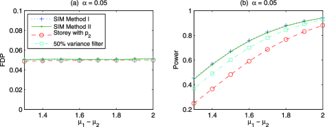
Figure 12: Calculated $\mathrm{FDP}$ and power of methods $\mathrm{I}$ and $\mathrm{II}$, the $50\%$ variance filter and the conventional $\mathrm{FDR}$ procedure (storey with $p_{2})$ for various size effect $\mu_{1}-\mu_{2}$ in Example $4$.

7 Integrative analysis on prostate cancer data

Genomic DNA copy number ($\mathrm{CN}$) alterations are key genetic events in the development and progression of human cancers. In parallel, microarray gene expression (GE) measurements of mRNA level provide an alternative for detecting some significant genes which contribute to certain cancer diseases. As discussed by the previous study Kimetal2007 , the amplified gene section was enriched with transcript overexpression, and the deleted section was enriched with mRNA downregulation. Hence, integration of $\mathrm{CN}$ aberration and GE to identify DNA $\mathrm{CN}$ alterations that induce changes in the expressional levels of the associated genes is a common task in cancer studies. To this end, several authors have explored integrative analysis of these two heterogeneous data sources to reveal higher levels of interactions that cannot be detected based on individual observations; see Lahtietal2013 and the references therein.

To demonstrate the practical utility of the $\mathrm{SIM}$ procedure, we applied it to data produced by Kimetal2007 in a study on prostate cancer progression. This study used an array comparative hybridization (aCGH) to profile genome-wide $\mathrm{CN}$ changes through the isolation of pure cell populations representing entire spectrum of prostate disease using laser capture microdissection (LCM) and OmniPlex Whole Genomic (WGA) Application. Data on $\mathrm{CN}$ alterations and GE were matched for $m=7534$ genes using prostate cell populations from low-grade ($n_{1}=27$) and high-grade samples ($n_{2}=17$) of cancerous tissue. We calculated two-sided $t$ statistics ($t_{1},t_{2}$) and their $p$-values ($p_{1},p_{2}$) for GE and $\mathrm{CN}$ aberrations for each of $7534$ genes. Here, the primary $p$-value $p_{2}$ was obtained from the copy number in DNA level and its transcriptional gene expression served as the preliminary $p$-value $p_{1}$. Panel (a) of Figure 13 shows the scatter plot of gene expression and copy number $p$-values, where the sample correlation coefficient of $p_{1}$ and $p_{2}$ is $-0.004$. This motivates us to apply our $\mathrm{SIM}$ method $\mathrm{I}$ to target the genes evidencing statistical significance in either DNA or mRNA level. Using the significance level $\alpha=0.01$, our $\mathrm{SIM}$ method $\mathrm{I}$ detects $174$ rejections with their geometric locations showing in panel (b) of Figure 13. The projection direction is estimated as $\hat{\theta}{}^{\mathrm{I}}=0.465$, supporting that the preliminary $p$-value from GE is informative.

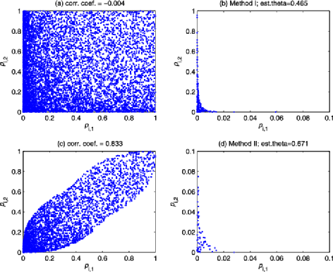
Figure 13: (a): Scatter plot of bivariate $p$-values $(p_{1},p_{2})$, where the correlation coefficient of $p_{1}$ and $p_{2}$ is $-0.004$; (b): geometric locations of the rejected genes using method $\mathrm{I}$ with the significance level $\alpha=0.01$. Here, the projection direction is $\hat{\theta}{}^{\mathrm{I}}=0.465$; (c): scatter plot of bivariate $p$-values $(p_{1},p_{2})$ of the trimmed genes, where the correlation coefficient of $p_{1}$ and $p_{2}$ is $0.833$; (d): geometric locations of the rejected genes using method $\mathrm{II}$ for the trimmed genes with the significance level $\alpha=0.01$. Here, the projection direction is $\hat{\theta}{}^{\mathrm{II}}=0.671$.

Note that our $\mathrm{SIM}$ procedure is valid for testing the conjunction of null hypotheses to favor genes with DNA copy number alterations or differential expressions under the alternative. Some genes are amplified or deleted in DNA level but have insignificant GE in mRNA level, which can be accounted for by the inappropriate use of “methylation;” while some upstream “transcription factor” genes found differentially expressed with activation (or suppression) function will up (or down) downstream genes. To further identify candidate genes with genetic alterations that accompany corresponding transcriptomic changes, we utilized a weight function, a product in DNA/RNA-Significance Analysis of Microarrays (DR-SAM) Salarietal2010 , to screen out the genes which are significant only in DNA or mRNA level. Specifically, the weight function, which is defined as $w=\min\{\frac{t_{1}}{t_{2}},\frac{t_{2}}{t_{1}}\}$ ($0\leq w\leq 1$), is the ratio of two $t$-scores. Small weight is applied to favor genes with unbalanced contributions on copy number and gene expression. Based on this rationale, the genes with weights larger than a threshold will serve as candidates for detecting concordantly altered genes. Given a threshold, the scatter plot of genes passing the threshold under the true null violates the normality and symmetry property assumptions. Fortunately, the genes with points above the line $p_{1}+p_{2}>1$ seldom come from the alternative. Hence, we modified the weight function on the area with $p_{1}+p_{2}>1$ as $w^{\prime}(p_{1},p_{2})=w(1-p_{1},1-p_{2})$ such that the genes passing the threshold satisfy the symmetry property assumption. A small threshold will enrich the alternative with some genes being significant only in DNA or mRNA level, increasing the false discovery rate; while a large threshold will screen out some genes exhibiting concordant changes, resulting in low power. Based on this perspective, the selection of the threshold using the modified weight function is fdr-power trade-off. For simplicity, we set the threshold such that $50\%$ of the genes will be screened out. Panel (c) of Figure 13 presents the scatter plot of the trimmed genes, which will be used for testing. At $\alpha=0.01$, our $\mathrm{SIM}$ method $\mathrm{II}$ estimates the projection direction as $\hat{\theta}{}^{\mathrm{II}}=0.671$ and selects $62$ genes, as shown in panel (d) of Figure 13. To make comprehensive comparisons, Table 4 shows the numbers of rejected genes by applying the $\mathrm{SIM}$ methods, and the three competing procedures as used in our numerical studies. In summary, all the three competing procedures with either $p_{1}$ or $p_{2}$ as primary $p$-values, are more conservative than our $\mathrm{SIM}$ procedures.

=253pt Methods Number of rejections $\mathrm{SIM}$ method $\mathrm{I}$ with the whole data $174$ $\mathrm{SIM}$ method $\mathrm{II}$ with the trimmed data $62$ Storey with $p_{1}$ $31$ Storey with $p_{2}$ $0$ Two-stage with $(p_{1}|p_{2})$ $16$ Two-stage with $(p_{2}|p_{1})$ $1$ Weighted $\mathrm{BH}$ with $(p_{1}|p_{2})$ $14$ Weighted $\mathrm{BH}$ with $(p_{2}|p_{1})$ $0$

Table 4: Compare the numbers of rejections by the $\mathrm{SIM}$ methods, the conventional $\mathrm{FDR}$ procedure (storey), the two-stage multiple testing procedure (two-stage), and the weighted multiple testing procedure (weighted $\mathrm{BH})$ when $\alpha=0.01$. Here, $(p_{i}|p_{j})$ indicates that $p_{i}$ is used as the primary $p$-value while $p_{j}$ serves as the preliminary $p$-value

Table 5: Summary of Gene Functional Classification from Gene Ontology $(\mathrm{GO})$. $9$ $\mathrm{GO}$ terms are inferred to be active using $\mathrm{MFA}$. Here, $\mathrm{P.MFA}$ represents the marginal posterior probability of activation, and basic statistics on these terms are provided in the “size” column (#prostate cancer-associated genes/set size)

$\bolds{\mathrm{GO}}$ ID	Gene set ($\bolds{\mathrm{GO}}$ term)	P.MFA	Size
GO:0007031	Peroxisome organization	0.7909023	2${}/{}$58
GO:0070307	Lens fiber cell development	0.7225289	1${}/{}$12
GO:0001569	Patterning of blood vessels	0.7094174	2${}/{}$35
GO:0001517	N-acetylglucosamine 6-O-sulfotransferase activity	0.7036159	1${}/{}$60
GO:0008455	Alpha-1, 6-mannosylglycoprotein	0.6962325	1${}/{}$10
GO:0043190	ATP-binding cassette (ABC) transporter complex	0.6593146	1${}/{}$60
GO:0008332	Low voltage-gated calcium channel activity	0.6440800	1${}/{}$30
GO:0030612	Arsenate reductase (thioredoxin) activity	0.6339682	1${}/{}$10
GO:0004464	Leukotriene-C4 synthase activity	0.6276624	1${}/{}$20

Of these $62$ genes selected by our $\mathrm{SIM}$ method $\mathrm{II}$ with the trimmed genes, $38$ were mapped to the official gene names (11,705 in total) for prostate cancer with somatic mutation listed on Catalogue of Somatic Mutation in Cancer (COSMIC), supporting these genes being putative oncogenes in prostate cancer. Notably, the top five genes, that is, ABCA4, ABCA3, ACTG1, AADAC and ACACA, were ranked as 426, 454, 700, 780 and $848$, respectively. Particularly, the gene ACACA, known to be involved in fatty and acid metabolism, was also identified in the previous study lapointeetal2004 . To integrate gene-set information from a complex system with our experimentally-derived gene list, a larger gene list is necessary. For this purpose, we performed our $\mathrm{SIM}$ method $\mathrm{II}$ to the trimmed genes at $\alpha=0.05$, which yields $331$ rejections. Among them, $102$ could be mapped to recognized genes by DAVID Huangetal2008 . To assess the functional content of this gene list, we applied a new approach termed as multifunctional analyzer ($\mathrm{MFA}$) proposed by Wangetal2013 , in the context of gene ontology terms. Compared with existing methods such as Fisher’s exact test and model-based gene-set analysis (MGSA) Baueretal2010 , $\mathrm{MFA}$ has the merit of alleviating the redundancy problem in Fisher’s exact test while improving the statistical efficiency of MGSA. Table 5 reports the gene sets which were inferred to be activated by $\mathrm{MFA}$ in prostate cancer.

8 Discussion

This paper proposes a $\mathrm{SIM}$ multiple testing procedure to embed prior information, such as the overall sample variance in a standard two-sample $t$ test in microarray experiments and the structurally spatial information for large-scale imaging data, into the conventional $\mathrm{FDR}$ procedure, by assuming the availability of a bivariate $p$-value for each null hypothesis. We discuss the optimal rejection region in terms of power comparison in a general bivariate model and project the bivariate $p$-value into a single-index quantified by a projection direction $\theta$. A novel procedure is established to estimate the optimal projection direction consistently under some mild conditions, followed by two procedures for the estimation and control of $\mathrm{FDR}$.

Although the operators $\Phi$ and $\Phi^{-1}$ in the single-index $p(\theta)$ come from the normality assumption, generalizations, such as $p(\theta)=\Psi(\cos(\theta)\Psi^{-1}(p_{1})+\sin(\theta)\Psi^{-1}(p_{2}))$, can be made, where $\Psi$ is the $\mathrm{CDF}$ of some random variable. We have shown in the simulation study that the normal operator $\Phi$ is robust to distributions of other bivariate test statistics. A thorough investigation of the role of the operator is beyond the scope of this paper, but could be of interest in the future research.

As discussed in Section 3, the essential spirit of multiple testing is on increasing the detection power while maintaining the $\mathrm{FDR}$ rigorously. Theoretically, the detection power is related to three quantities, that is, $\pi_{0}$, $F_{0}(t)$ and $F_{1}(t)$, via the Bayesian $\mathrm{Fdr}$ formula $F_{1}(t)=({1}/{\alpha}-1){\pi_{0}}/{\pi_{1}}F_{0}(t)$. Screening out a proportion of uninformative hypotheses by an effective filter will enrich for nonnull hypotheses while simultaneously reducing the number of hypotheses to be tested at the second stage. From this point of view, the independence filter provided by Bourgonetal2010 aims to decrease $\pi_{0}$ to improve the detection power. However, in our $\mathrm{SIM}$ multiple testing procedure, we project the bivariate $p$-value into a single-index, which significantly changes the true null and nonnull distributions $(F_{0}(t),F_{1}(t))$. Hence, the power is increased by changing the structure of $p$-values while keeping $\pi_{0}$ to be constant. Our future research will be focused on constructing a more powerful multiple testing procedure via reducing the proportion of true null hypothesis and changing the structure of $p$-values simultaneously.

Beyond the weak dependence assumption made in (C2), the sequence of the projected $p$-values will inevitably inherit strong dependence from the primary test statistics, making the $\mathrm{SIM}$ procedure less accurate. Much published work has been developed to handle multiple testing problem with some strong dependence structure; see Fanetal2012 and the references therein. Much research is needed to investigate the performance of the $\mathrm{SIM}$ methods for solving multiple testing problem with strong dependence structure across the tests.

Appendix A Proofs of main results

For presentational fluency, denote $\widetilde{F}_{0}(t,\theta)={V(t,\theta)}/{m_{0}}$, $\widetilde{F}_{1}(t,\theta)=\break\{R(t,\theta)-V(t,\theta)\}/{m_{1}}$ and $\widehat{F}(t,\theta)=R(t,\theta)/m$. Analogously, define the following left-limit processes:

$$\widetilde{F}_{0}(t-,\theta) = m_{0}^{-1}\sum_{i=1}^{m}\mathrm{I}\bigl{\{}p_{i}(\theta)<t,H_{0}(i)\bigr{\}},$$

$$\widetilde{F}_{1}(t-,\theta) = m_{1}^{-1}\sum_{i=1}^{m}\mathrm{I}\bigl{\{}p_{i}(\theta)<t,H_{1}(i)\bigr{\}},$$

$$\widehat{F}(t-,\theta) = m^{-1}\sum_{i=1}^{m}\mathrm{I}\bigl{\{}p_{i}(\theta)<t\bigr{\}}.$$

We only prove the main results involved the nonparametric estimator $\widehat{F}_{0}^{\mathrm{II}}(t,\theta)$. For those involved the parametric estimator $\widehat{F}_{0}^{\mathrm{I}}(t,\theta)$, all proofs will go through as long as this estimator uniformly converges to the true null distribution $F_{0}(t,\theta)$ for all $t$ and $\theta$.

We first impose some regularity conditions, which are not the weakest possible but facilitate the technical derivations.

Conditions

[(C10)]

$\lim_{m\to\infty}m_{0}/m=\pi_{0}$ exists and $0<\pi_{0}<1$.

$\lim_{m\to\infty}{m_{0}}^{-1}{\sum_{i=1}^{m}\mathrm{I}(p_{ij}\leq t,H_{0}(i))}=G_{0}^{j}(t)$ and $\lim_{m\to\infty}{m_{1}}^{-1}\*{\sum_{i=1}^{m}\mathrm{I}(p_{ij}\leq t,H_{1}(i))}=G_{1}^{j}(t)$ almost surely, for $j=1,2$.

For any rational number $\alpha\in[0,1]$, denote by $q_{\alpha}(\theta)$ the $100\alpha$th quantile of the distribution function $F(t,\theta)$. Assume that $\widehat{F}(t,\theta)$ and$F(t,\theta)$ satisfy the Lipschitz continuity as follows: $\sup_{m}\sup_{\alpha}|\widehat{F}(q_{\alpha}(\theta),\theta)-\break\widehat{F}(q_{\alpha}(\theta^{\prime}),\theta^{\prime})|\leq C_{1}|\theta-\theta^{\prime}|$ and $\sup_{\alpha}|F(q_{\alpha}(\theta),\theta)-F(q_{\alpha}(\theta^{\prime}),\theta^{\prime})|\leq C_{1}|\theta-\theta^{\prime}|$, where $C_{1}$ is a generic positive constant, not depending on $\widehat{F},F$ and $\alpha$. The Lipschitz continuity conditions also hold for $\widehat{F}(t-,\theta)$ and $F(t-,\theta)$. In addition, $F_{0}(t,\theta)$, $F_{0}(t-,\theta)$, $\widetilde{F}_{0}(t,\theta)$ and $\widetilde{F}_{0}(t-,\theta)$ satisfy the Lipschitz continuity conditions.

The probability density function of $(p_{1},p_{2})$ under the true null is centrally symmetric with respect to $(1/2,1/2)$.

$F_{1}({1}/{2},\theta)=1$ for all $\theta$.

$\inf_{\theta}F(\delta,\theta)>0$, for any $\delta>0$.

$F_{0}(t,\theta)$ and $F(t,\theta)$ are continuous in the region $\{(t,\theta)\dvtx t^{*}_{\alpha^{\prime}}(\theta)\leq t\leq 1\}$ and $|F(t,\theta)-F(t^{*}_{\alpha^{\prime}}(\theta),\theta)|\leq C_{2}|t-t^{*}_{\alpha^{\prime}}(\theta)|$, where $C_{2}$ is a constant not depending on $\theta$.

$$\lim_{t\to t^{*}_{\alpha^{\prime}}(\theta)}\frac{F_{0}(t,\theta)/F(t,\theta)-F_{0}(t^{*}_{\alpha^{\prime}}(\theta),\theta)/F(t^{*}_{\alpha^{\prime}}(\theta),\theta)}{t-t^{*}_{\alpha^{\prime}}(\theta)}=k(\theta)$$

uniformly for $\theta$, where $\inf_{\theta}|k(\theta)|>0$.

(Identification). Given $\delta^{\prime}>0$, there exists $\varepsilon>0$, such that

$$\inf_{\theta\dvtx|\theta-\theta_{0}(\alpha^{\prime})|>\delta^{\prime}}\bigl{\{}F\bigl{(}t^{*}_{\alpha^{\prime}}\bigl{(}\theta_{0}(\alpha^{\prime})\bigr{)},\theta_{0}(\alpha^{\prime})\bigr{)}-F\bigl{(}t^{*}_{\alpha^{\prime}}(\theta),\theta\bigr{)}\bigr{\}}\geq\varepsilon.$$

$|F(t,\theta)-F(t,\theta_{0}(\alpha^{\prime}))|\leq C_{3}|\theta-\theta_{0}(\alpha^{\prime})|$ and $|F_{0}(t,\theta)-F_{0}(t,\theta_{0}(\alpha^{\prime}))|\leq C_{3}|\theta-\theta_{0}(\alpha^{\prime})|$, where $C_{3}$ is a constant not depending on $\theta$ and $t$.

Before proving the propositions and theorems, we first show Lemmas 1 and 2.

Lemma 1

Assume conditions (C1) to (C3). Let $p_{i}(\theta)\,{=}\,\Phi(\cos(\theta)\Phi^{-1}(p_{i1})\!+\sin(\theta)\Phi^{-1}(p_{i2}))$, $i=1,\ldots,m$, where $\Phi$ is the $\mathrm{CDF}$ of a standard normal random variable. Then we have

$$\sup_{0\leq\theta\leq{\pi}/{2}}\sup_{0\leq t\leq 1}\Biggl{|}\frac{1}{m_{0}}\sum_{i=1}^{m}\mathrm{I}\bigl{\{}p_{i}(\theta)\leq t,H_{0}(i)\bigr{\}}-F_{0}(t,\theta)\Biggr{|} \stackrel{{\scriptstyle\mathit{a.s.}}}{{\to}} 0,$$

$$\sup_{0\leq\theta\leq{\pi}/{2}}\sup_{0\leq t\leq 1}\Biggl{|}\frac{1}{m_{1}}\sum_{i=1}^{m}\mathrm{I}\bigl{\{}p_{i}(\theta)\leq t,H_{1}(i)\bigr{\}}-F_{1}(t,\theta)\Biggr{|} \stackrel{{\scriptstyle\mathit{a.s.}}}{{\to}} 0,$$

$$\sup_{0\leq\theta\leq{\pi}/{2}}\sup_{0\leq t\leq 1}\Biggl{|}\frac{1}{m}\sum_{i=1}^{m}\mathrm{I}\bigl{\{}p_{i}(\theta)\leq t\bigr{\}}-F(t,\theta)\Biggr{|} \stackrel{{\scriptstyle\mathit{a.s.}}}{{\to}} 0.$$

We first show the uniform consistency of $\widehat{F}(t,\theta)$. For fixed $t$ and $\theta$, $\{p_{i}(\theta)\dvtx i=1,\ldots,m\}$ satisfy the weak dependence:

$$\Biggl{|}\frac{1}{m}\sum_{i=1}^{m}\mathrm{I}\bigl{\{}p_{i}(\theta)\leq t\bigr{\}}-F(t,\theta)\Biggr{|} \stackrel{{\scriptstyle\mathrm{a.s.}}}{{\to}} 0,$$

$$\Biggl{|}\frac{1}{m}\sum_{i=1}^{m}\mathrm{I}\bigl{\{}p_{i}(\theta)<t\bigr{\}}-F(t-,\theta)\Biggr{|} \stackrel{{\scriptstyle\mathrm{a.s.}}}{{\to}} 0.$$

This conclusion is directly implied by conditions (C1) and (C2). To prove the uniform consistency of $\widehat{F}(t,\theta)$, we extend the argument in the proof of the Glivenko–Cantelli theorem Durrett2010 . For $0\leq j\leq k$, partitioning the domain into grid points $(t,\theta)$ as $\{q_{j/k}(\theta_{l})\dvtx j=0,\ldots,k;l=0,\ldots,L_{k}\}$ such that $\{\theta_{l}\dvtx l=0,\ldots,L_{k}\}$ are equally spaced in $[0,\pi/2]$ with unit length less than or equal to ${1}/{(C_{1}k)}$, where $C_{1}$ is given in condition (C3). The pointwise convergence (A) implies that we can pick up $N_{k}(\omega)$ such that

$$\bigl{|}\widehat{F}\bigl{(}q_{j/k}(\theta_{l}),\theta_{l}\bigr{)}-F\bigl{(}q_{j/k}(\theta_{l}),\theta_{l}\bigr{)}\bigr{|} < k^{-1}\quad\mbox{and}$$

$$\bigl{|}\widehat{F}\bigl{(}q_{j/k}(\theta_{l})-,\theta_{l}\bigr{)}-F\bigl{(}q_{j/k}(\theta_{l})-,\theta_{l}\bigr{)}\bigr{|} < k^{-1}$$

for $0\leq j\leq k$ and $0\leq l\leq L_{k}$. For $t\in(q_{{(j-1)}/k}(\theta),q_{{j}/k}(\theta))$ and $\theta\in(\theta_{l-1},\theta_{l})$ with $1\leq j\leq k$, $1\leq l\leq L_{k}$ and $m>N_{k}(\omega)$, using the monotonicity of $\widehat{F}$ and $F$, $F(q_{j/k}(\theta)-,\theta)-F(q_{{j-1}/k}(\theta),\theta)\leq k^{-1}$ and condition (C3), we have

$$\widehat{F}(t,\theta) \leq \widehat{F}\bigl{(}q_{j/k}(\theta)-,\theta\bigr{)}$$

$$\leq \widehat{F}\bigl{(}q_{j/k}(\theta_{l-1})-,\theta_{l-1}\bigr{)}+k^{-1}$$

$$\leq F\bigl{(}q_{j/k}(\theta_{l-1})-,\theta_{l-1}\bigr{)}+2k^{-1}$$

$$\leq F\bigl{(}q_{{j-1}/k}(\theta_{l-1}),\theta_{l-1}\bigr{)}+3k^{-1}$$

$$\leq F\bigl{(}q_{{j-1}/k}(\theta),\theta\bigr{)}+4k^{-1}$$

$$\leq F(t,\theta)+4k^{-1}.$$

Similar arguments lead to $\widehat{F}(t,\theta)\geq F(t,\theta)-4k^{-1}$. So $\sup_{\theta}\sup_{t}|\widehat{F}(t,\theta)-F(t,\theta)|\leq 4k^{-1}$, and we have proved the result. The uniform convergence of $\widetilde{F}_{0}(t,\theta)$ can be derived similarly. Combining these two results, we obtain the uniform convergence of $\widetilde{F}_{1}(t,\theta)$ immediately.

Lemma 2

Under conditions (C1)–(C5), the nonparametric estimator $\widehat{F}_{0}^{\mathrm{II}}(t,\theta)$ uniformly converges to $F_{0}(t,\theta)$ for all $t$ and $\theta$.

Proof of Proposition 1 Let $\mathrm{I}(\mathbf{p}\in\mathbf{S}_{\mathrm{OR}})$ be the indicator of $\mathbf{p}\in\mathbf{S}_{\mathrm{OR}}$ and $\mathrm{I}(\mathbf{p}\in\mathbf{S})$ be the indicator of $\mathbf{p}\in\mathbf{S}$ for any rejection region satisfying $\mathrm{Fdr}(\mathbf{S})\leq\alpha$. Since $\mathrm{Fdr}(\mathbf{S}_{\mathrm{OR}})$ is the conditional expectation of $\mathrm{fdr}(\mathbf{p})$ given $\mathbf{p}\in\mathbf{S}_{\mathrm{OR}}$ EfronTibshirani2002 , some derivations yield that

$$\alpha = \mathrm{Fdr}(\mathbf{S}_{\mathrm{OR}})=E_{f}\bigl{\{}\mathrm{fdr}(\mathbf{p})|\mathbf{p}\in\mathbf{S}_{\mathrm{OR}}\bigr{\}}$$

$$= \int_{\{\mathbf{p}\dvtx\mathrm{fdr}(\mathbf{p})<C\}}\mathrm{fdr}(\mathbf{p})\,d\widetilde{\mathbf{P}}+\int_{\{\mathbf{p}\dvtx\mathrm{fdr}(\mathbf{p})=C\}}\mathrm{fdr}(\mathbf{p})\,d\widetilde{\mathbf{P}}$$

$$= \int_{\{\mathbf{p}\dvtx\mathrm{fdr}(\mathbf{p})<C\}}\mathrm{fdr}(\mathbf{p})\,d\widetilde{\mathbf{P}}<C,$$

where $\widetilde{\mathbf{P}}$ denotes the probability measure of $\mathbf{p}$ given $\mathbf{p}\in\mathbf{S}_{\mathrm{OR}}$ and the last equality holds by condition (9). As a result, $C>0$ and $1-\alpha/C>0$. By condition (9), there exists $\mathbf{S}^{\prime}$ such that $\mathbf{S}\subseteq\mathbf{S}^{\prime}$ and $\mathrm{Fdr}(\mathbf{S}^{\prime})=\alpha$. For every $\mathbf{p}$,

$$\mathrm{I}\bigl{(}\mathbf{p}\in\mathbf{S}^{\prime}\bigr{)}\bigl{\{}1-\mathrm{fdr}(\mathbf{p})/C\bigr{\}}\leq\mathrm{I}(\mathbf{p}\in\mathbf{S}_{\mathrm{OR}})\bigl{\{}1-\mathrm{fdr}(\mathbf{p})/C\bigr{\}},$$ (34)

where (34) is based on the observation that if $\mathbf{p}\notin\mathbf{S}_{\mathrm{OR}}$, the left-hand side of (34) is less than or equal to zero. By taking expectation for both sides of equation (34),

$$\int\mathrm{I}\bigl{(}\mathbf{p}\in\mathbf{S}^{\prime}\bigr{)}\bigl{\{}1-\mathrm{fdr}(\mathbf{p})/C\bigr{\}}f(\mathbf{p})\,d\mathbf{p}\leq\int\mathrm{I}(\mathbf{p}\in\mathbf{S}_{\mathrm{OR}})\bigl{\{}1-\mathrm{fdr}(\mathbf{p})/C\bigr{\}}f(\mathbf{p})\,d\mathbf{p},$$

we obtain the following inequality:

$$F\bigl{(}\mathbf{S}^{\prime}\bigr{)}\bigl{\{}1-\mathrm{Fdr}\bigl{(}\mathbf{S}^{\prime}\bigr{)}/C\bigr{\}}\leq F(\mathbf{S}_{\mathrm{OR}})\bigl{\{}1-\mathrm{Fdr}(\mathbf{S}_{\mathrm{OR}})/C\bigr{\}},$$ (35)

where $F(\mathbf{S})=\pi_{0}F_{0}(\mathbf{S})+\pi_{1}F_{1}(\mathbf{S})$. By definition, both $1-\mathrm{Fdr}(\mathbf{S}^{\prime})/C$ and $1-\mathrm{Fdr}(\mathbf{S}_{\mathrm{OR}})/C$ are equal to $1-\alpha/C>0$. Hence, (35) implies that $F(\mathbf{S}^{\prime})\leq F(\mathbf{S}_{\mathrm{OR}})$. From the $\mathrm{Fdr}$ formula, $F(\mathbf{S}^{\prime})={\pi_{1}}/{(1-\alpha)}F_{1}(\mathbf{S}^{\prime})$ and $F(\mathbf{S}_{\mathrm{OR}})={\pi_{1}}/{(1-\alpha)}F_{1}(\mathbf{S}_{\mathrm{OR}})$. So $F_{1}(\mathbf{S}^{\prime})\leq F_{1}(\mathbf{S}_{\mathrm{OR}})$. The proof is completed by the fact that $F_{1}(\mathbf{S})\leq F_{1}(\mathbf{S}^{\prime})$ for any $\mathbf{S}\subseteq\mathbf{S}^{\prime}$.

Proof of Proposition 2 By continuity, $t^{*}_{\alpha^{\prime}}(\theta)$ satisfies that $F_{0}(t,\theta)/\break F(t,\theta)=\alpha^{\prime}$. From the $\mathrm{Fdr}$ formula, for any $\theta$, $t^{*}_{\alpha^{\prime}}(\theta)$ is the solution of the equation $F_{1}(t,\theta)=\beta F_{0}(t,\theta)$. Since $\frac{\partial F_{1}(t,\theta)}{\partial t}-\beta\frac{\partial F_{0}(t,\theta)}{\partial t}\neq 0$ for any interior point $(t,\theta,\alpha^{\prime})$ in $[0,1]\times[0,\pi/2]\times[0,1/\pi_{0}]$, implicit function theorem implies that there exists a unique continuously differentiable function $t=g(\alpha^{\prime},\theta)$ such that $F_{1}(g(\alpha^{\prime},\theta),\theta)=\beta F_{0}(g(\alpha^{\prime},\theta),\theta)$. By uniqueness, $t^{*}_{\alpha^{\prime}}(\theta)=g(\alpha^{\prime},\theta)$, indicating that $t^{*}_{\alpha^{\prime}}(\theta)$ is continuously differentiable with respect to $\theta$ and $\alpha^{\prime}$. Taking derivative with respect to $\theta$ for both sides of $F_{1}(t^{*}_{\alpha^{\prime}}(\theta),\theta)=\beta F_{0}(t^{*}_{\alpha^{\prime}}(\theta),\theta)$ leads to

$$\biggl{\{}\frac{\partial F_{1}(t,\theta)}{\partial t}\frac{\partial t^{*}_{\alpha^{\prime}}(\theta)}{\partial\theta}+\frac{\partial F_{1}(t,\theta)}{\partial\theta}\biggr{\}}\bigg{|}_{t=t^{*}_{\alpha^{\prime}}(\theta)}$$

(36)

$$\qquad=\biggl{\{}\beta\frac{\partial F_{0}(t,\theta)}{\partial t}\frac{\partial t^{*}_{\alpha^{\prime}}(\theta)}{\partial\theta}+\beta\frac{\partial F_{0}(t,\theta)}{\partial\theta}\biggr{\}}\bigg{|}_{t=t^{*}_{\alpha^{\prime}}(\theta)}.$$

From (A), $\frac{\partial t^{*}_{\alpha^{\prime}}(\theta)}{\partial\theta}$ can be expressed as

$$\frac{\partial t^{*}_{\alpha^{\prime}}(\theta)}{\partial\theta}=\biggl{\{}\frac{\beta(({\partial F_{0}(t,\theta)})/({\partial\theta}))-(({\partial F_{1}(t,\theta)})/({\partial\theta}))}{(({\partial F_{1}(t,\theta)})/({\partial t}))-\beta(({\partial F_{0}(t,\theta)})/({\partial t}))}\biggr{\}}\bigg{|}_{t=t^{*}_{\alpha^{\prime}}(\theta)}.$$ (37)

Since $F_{1}(t^{*}_{\alpha^{\prime}}(\theta),\theta)$ achieves the maximum at $\theta_{0}(\alpha^{\prime})$, the following partial differential equation holds, that is,

$$\biggl{[}\biggl{\{}\frac{\partial F_{1}(t,\theta)}{\partial t}\frac{\partial t^{*}_{\alpha^{\prime}}(\theta)}{\partial\theta}+\frac{\partial F_{1}(t,\theta)}{\partial\theta}\biggr{\}}\bigg{|}_{t=t^{*}_{\alpha^{\prime}}(\theta)}\biggr{]}\bigg{|}_{\theta=\theta_{0}(\alpha^{\prime})}=0.$$ (38)

Plugging (37) into (38), the partial differential equation can be simplified as

$$\biggl{[}\biggl{\{}\frac{\partial F_{1}(t,\theta)}{\partial t}\Big{/}\frac{\partial F_{1}(t,\theta)}{\partial\theta}\biggr{\}}\bigg{|}_{t=t^{*}_{\alpha^{\prime}}(\theta)}\biggr{]}\bigg{|}_{\theta=\theta_{0}(\alpha^{\prime})}$$

(39)

$$\qquad=\biggl{[}\biggl{\{}\frac{\partial F_{0}(t,\theta)}{\partial t}\Big{/}\frac{\partial F_{0}(t,\theta)}{\partial\theta}\biggr{\}}\bigg{|}_{t=t^{*}_{\alpha^{\prime}}(\theta)}\biggr{]}\bigg{|}_{\theta=\theta_{0}(\alpha^{\prime})}.$$

From $(\ref{A8})$, the $x$-coordinate of the point of intersection of the solution set $\{(\theta,t)\}$ satisfying (22) and $t=t^{*}_{\alpha^{\prime}}(\theta)$ is $\theta_{0}(\alpha^{\prime})$.

“$\Leftarrow$”: $\theta_{0}(\alpha^{\prime})$ is constant for all $0<\alpha^{\prime}<1/\pi_{0}$ if the solution $\theta$ of $t$ of the equation (22) is unique and equals a constant.

“$\Rightarrow$”: If the solution $\theta$ of $t$ of the equation (22) is either not unique or not equal to a constant, then there exists $t_{1}$ and $t_{2}$ such that $\theta(t_{1})\neq\theta(t_{2})$. Since $t^{*}_{\alpha^{\prime}}(\theta)$ are continuous and nondecreasing from $[0,1/\pi_{0}]$ with respect to $\alpha^{\prime}$ for any $\theta$, there exists $\alpha^{\prime}_{1}$ and $\alpha^{\prime}_{2}$ such that $t^{*}_{\alpha^{\prime}_{1}}(\theta(t_{1}))=t_{1}$ and $t^{*}_{\alpha^{\prime}_{2}}(\theta(t_{2}))=t_{2}$. From (A), $\theta(t_{1})=\theta_{0}(\alpha^{\prime}_{1})$ and $\theta(t_{2})=\theta_{0}(\alpha^{\prime}_{2})$, which implies that $\theta_{0}(\alpha^{\prime})$ is not constant for all $0<\alpha^{\prime}<1/\pi_{0}$.

Under the normality assumption, $F_{1}(t,\theta)=\Phi(\frac{\Phi^{-1}(t)-\mu_{1}(\theta)}{\sigma_{0}(\theta)})$ and $F_{0}(t,\theta)=\Phi(\frac{\Phi^{-1}(t)-\mu_{0}(\theta)}{\sigma_{0}(\theta)})$, where $\mu_{0}(\theta)=\mu_{0;1}\cos(\theta)+\mu_{0;2}\sin(\theta)$, $\mu_{1}(\theta)=\mu_{1;1}\cos(\theta)+\mu_{1;2}\sin(\theta)$ and $\sigma_{0}(\theta)$ is appearing in (17). In this case, (A) reduces to $[\frac{\partial}{\partial\theta}\{\frac{\mu_{0}(\theta)}{\sigma_{0}(\theta)}\}=\frac{\partial}{\partial\theta}\{\frac{\mu_{1}(\theta)}{\sigma_{0}(\theta)}\}]{|}_{\theta=\theta_{0}(\alpha^{\prime})}$, implying that $\theta_{0}(\alpha^{\prime})$ is constant.

Proof of Proposition 3 For left-sided hypotheses, the joint $\mathrm{CDF}$ of $(\tilde{p}_{1},p_{2})$ under the true null can be derived as

$$\mathrm{P}(\tilde{p}_{1}\leq\tilde{t}_{1},p_{2}\leq t_{2}|H_{0})$$

$$\qquad=\mathrm{P}\bigl{(}F_{0;X_{1}}(\widetilde{X}_{1})\leq\tilde{t}_{1},p_{2}\leq t_{2}|H_{0}\bigr{)}$$

$$\qquad=\mathrm{P}\bigl{(}p_{1}\leq F_{0;X_{1}}\bigl{(}F_{0;X_{1}}^{-1}(\tilde{t}_{1})-\eta\bigr{)},p_{2}\leq t_{2}|H_{0}\bigr{)}$$

$$\qquad=\int_{-\infty}^{\infty}f_{\eta}(\eta)\biggl{\{}\int_{0}^{F_{0;X_{1}}(F_{0;X_{1}}^{-1}(\tilde{t}_{1})-\eta)}\int_{0}^{t_{2}}f_{0;(p_{1},p_{2})}(p_{1},p_{2})\,dp_{1}\,dp_{2}\biggr{\}}\,d\eta,$$

where $f_{\eta}$ is the p.d.f. of $\eta$, $f_{0;(p_{1},p_{2})}$ is the p.d.f. of $(p_{1},p_{2})$ under the true null, and $F_{0;X_{1}}^{-1}$ is the inverse function of $F_{0;X_{1}}$. By taking derivatives of (A), we obtain

$$f_{0;(\tilde{p}_{1},p_{2})}(\tilde{p}_{1},p_{2})$$

$$\qquad=\int_{-\infty}^{\infty}f_{\eta}(\eta)\frac{f_{0;X_{1}}(F_{0;X_{1}}^{-1}(\tilde{p}_{1})-\eta)}{f_{0;X_{1}}(F_{0;X_{1}}^{-1}(\tilde{p}_{1}))}$$ (41)

$$\hskip 52.0pt{}\times f_{0;(p_{1},p_{2})}\bigl{(}F_{0;X_{1}}\bigl{(}F_{0;X_{1}}^{-1}(\tilde{p}_{1})-\eta\bigr{)},p_{2}\bigr{)}\,d\eta,$$

where $f_{0;(\tilde{p}_{1},p_{2})}$ is the p.d.f. of $(\tilde{p}_{1},p_{2})$ under the true null and $f_{0;X_{1}}$ is the true null p.d.f. of $X_{1}$. Thus,

$$f_{0;(\tilde{p}_{1},p_{2})}(1-\tilde{p}_{1},1-p_{2})$$

$$\qquad=\int_{-\infty}^{\infty}f_{\eta}(\eta)\frac{f_{0;X_{1}}(F_{0;X_{1}}^{-1}(1-\tilde{p}_{1})-\eta)}{f_{0;X_{1}}(F_{0;X_{1}}^{-1}(1-\tilde{p}_{1}))}$$

$$\hskip 53.0pt{}\times f_{0;(p_{1},p_{2})}\bigl{(}F_{0;X_{1}}\bigl{(}F_{0;X_{1}}^{-1}(1-\tilde{p}_{1})-\eta\bigr{)},1-p_{2}\bigr{)}\,d\eta$$

$$\qquad=\int_{-\infty}^{\infty}f_{\eta}(\eta)\frac{f_{0;X_{1}}(-F_{0;X_{1}}^{-1}(\tilde{p}_{1})-\eta)}{f_{0;X_{1}}(-F_{0;X_{1}}^{-1}(\tilde{p}_{1}))}$$

(42)

$$\hskip 53.0pt{}\times f_{0;(p_{1},p_{2})}\bigl{(}F_{0;X_{1}}\bigl{(}-F_{0;X_{1}}^{-1}(\tilde{p}_{1})-\eta\bigr{)},1-p_{2}\bigr{)}\,d\eta$$

$$\qquad=\int_{-\infty}^{\infty}f_{\eta}(\eta)\frac{f_{0;X_{1}}(F_{0;X_{1}}^{-1}(\tilde{p}_{1})+\eta)}{f_{0;X_{1}}(F_{0;X_{1}}^{-1}(\tilde{p}_{1}))}$$

(43)

$$\hskip 53.0pt{}\times f_{0;(p_{1},p_{2})}\bigl{(}1-F_{0;X_{1}}\bigl{(}F_{0;X_{1}}^{-1}(\tilde{p}_{1})+\eta\bigr{)},1-p_{2}\bigr{)}\,d\eta$$

$$\qquad=\int_{-\infty}^{\infty}f_{\eta}(\eta)\frac{f_{0;X_{1}}(F_{0;X_{1}}^{-1}(\tilde{p}_{1})+\eta)}{f_{0;X_{1}}(F_{0;X_{1}}^{-1}(\tilde{p}_{1}))}$$

(44)

$$\hskip 53.0pt{}\times f_{0;(p_{1},p_{2})}\bigl{(}F_{0;X_{1}}\bigl{(}F_{0;X_{1}}^{-1}(\tilde{p}_{1})+\eta\bigr{)},p_{2}\bigr{)}\,d\eta$$

$$\qquad=\int_{-\infty}^{\infty}f_{\eta}(-\eta)\frac{f_{0;X_{1}}(F_{0;X_{1}}^{-1}(\tilde{p}_{1})-\eta)}{f_{0;X_{1}}(F_{0;X_{1}}^{-1}(\tilde{p}_{1}))}$$

$$\hskip 53.0pt{}\times f_{0;(p_{1},p_{2})}\bigl{(}F_{0;X_{1}}\bigl{(}F_{0;X_{1}}^{-1}(\tilde{p}_{1})-\eta\bigr{)},p_{2}\bigr{)}\,d\eta$$

$$\qquad=\int_{-\infty}^{\infty}f_{\eta}(\eta)\frac{f_{0;X_{1}}(F_{0;X_{1}}^{-1}(\tilde{p}_{1})-\eta)}{f_{0;X_{1}}(F_{0;X_{1}}^{-1}(\tilde{p}_{1}))}$$

(45)

$$\hskip 53.0pt{}\times f_{0;(p_{1},p_{2})}\bigl{(}F_{0;X_{1}}\bigl{(}F_{0;X_{1}}^{-1}(\tilde{p}_{1})-\eta\bigr{)},p_{2}\bigr{)}\,d\eta,$$

where (42) and (43) are due to the fact that $f_{0;X_{1}}$ is symmetric with respect to 0, (44) is satisfied by using the symmetry property assumption on $f_{0;(p_{1},p_{2})}(p_{1},p_{2})$, and (45) holds under the assumption that the p.d.f. of $\eta$ is symmetric. (A) together with (45) yields that

$$f_{0;(\tilde{p}_{1},p_{2})}(\tilde{p}_{1},p_{2})=f_{0;(\tilde{p}_{1},p_{2})}(1-\tilde{p}_{1},1-p_{2}),$$

for any $\tilde{p}_{1}$ and $p_{2}$ in $[0,1]\times[0,1]$. The case for right-sided hypotheses can be derived in a similar way. These complete the proof.

Proof of Theorem 1 Before proving Theorem 1, we first provide Lemma 3.

Lemma 3

Under conditions (C1) to (C8),

$$\sup_{\theta}\bigl{|}\hat{t}{}_{\alpha^{\prime}}^{*\mathrm{II}}(\theta)-t^{*}_{\alpha^{\prime}}(\theta)\bigr{|}\stackrel{{\scriptstyle\mathit{a.s.}}}{{\to}}0.$$

Fix $\delta_{1}>0$, and let $\bar{t}(\theta)$ be any curve such that $t^{*}_{\alpha^{\prime}}(\theta)+\delta_{1}\leq\bar{t}(\theta)\leq 1$. Then

$$\frac{\widehat{F}_{0}^{{\mathrm{II}}}(\bar{t}(\theta),\theta)}{\{R(\bar{t}(\theta),\theta)\vee 1\}/m}$$

$$\qquad\geq\frac{F_{0}(\bar{t}(\theta),\theta)-|\widehat{F}_{0}^{{\mathrm{II}}}(\bar{t}(\theta),\theta)-F_{0}(\bar{t}(\theta),\theta)|}{F(\bar{t}(\theta),\theta)+|\{R(\bar{t}(\theta),\theta)\vee 1\}/m-F(\bar{t}(\theta),\theta)|}$$

$$\qquad\geq\frac{\inf_{\theta}F_{0}(\bar{t}(\theta),\theta)/F(\bar{t}(\theta),\theta)-\epsilon_{1}}{1+\epsilon_{2}},$$

where $\epsilon_{1}=\inf_{\theta}\inf_{t\geq\delta_{1}}|\widehat{F}_{0}^{{\mathrm{II}}}(t,\theta)-F_{0}(t,\theta)|/F(t,\theta)$, and

$$\epsilon_{2}=\sup_{\theta}\sup_{t\geq\delta_{1}}\bigl{|}\bigl{\{}R(t,\theta)\vee 1\bigr{\}}/m-F(t,\theta)\bigr{|}/F(t,\theta).$$

By Lemmas 1, 2 and condition (C6), $\epsilon_{1}\stackrel{{\scriptstyle\mathrm{a.s.}}}{{\to}}0$ and $\epsilon_{2}\stackrel{{\scriptstyle\mathrm{a.s.}}}{{\to}}0$. Note that $F_{0}(\bar{t}(\theta),\theta)/\break F(\bar{t}(\theta),\theta)>\alpha^{\prime}$; otherwise it contradicts $t^{*}_{\alpha^{\prime}}(\theta)$ being supremum. By condition (C7), $\inf_{\theta}F_{0}(\bar{t}(\theta),\theta)/F(\bar{t}(\theta),\theta)>\alpha^{\prime}$. Hence, for a sufficiently large $M_{1}(\delta_{1})$, when $m>M_{1}(\delta_{1})$, if follows that

$$m\widehat{F}_{0}^{{\mathrm{II}}}\bigl{(}\bar{t}(\theta),\theta\bigr{)}/\bigl{\{}R\bigl{(}\bar{t}(\theta),\theta\bigr{)}\vee 1\bigr{\}}>\alpha^{\prime}$$

with probability $1$, which implies that $\hat{t}{}_{\alpha^{\prime}}^{*\mathrm{II}}(\theta)\leq t^{*}_{\alpha^{\prime}}(\theta)+\delta_{1}$ almost surely.

On the other hand, by condition (C8), since ${F_{0}(t,\theta)}/{F(t,\theta)}$ has a nonzero derivative $k(\theta)$ at $t^{*}_{\alpha^{\prime}}(\theta)$, it must be positive; otherwise $t^{*}_{\alpha^{\prime}}(\theta)$ cannot be the true supremum for all $t$ such that ${F_{0}(t,\theta)}/{F(t,\theta)}\leq\alpha^{\prime}$. For any $\varepsilon>0$, there exists $\xi>\delta_{1}$ such that, for $|\tilde{t}(\theta)-t^{*}_{\alpha^{\prime}}(\theta)|\leq\xi$,

$$\biggl{|}\frac{F_{0}(\tilde{t}(\theta),\theta)/F(\tilde{t}(\theta),\theta)-F_{0}(t^{*}_{\alpha^{\prime}}(\theta),\theta)/F(t^{*}_{\alpha^{\prime}}(\theta),\theta)}{\tilde{t}(\theta)-t^{*}_{\alpha^{\prime}}(\theta)}-k(\theta)\biggr{|}<\varepsilon.$$

For a truncated area with $t^{*}_{\alpha^{\prime}}(\theta)-\xi\leq\tilde{t}(\theta)\leq t^{*}_{\alpha^{\prime}}(\theta)-\delta_{1}$, $\sup_{\theta}{F_{0}(\tilde{t}(\theta),\theta)}/\break{F(\tilde{t}(\theta),\theta)}<\alpha^{\prime}$. When $\tilde{t}(\theta)\in[t^{*}_{\alpha^{\prime}}(\theta)-\xi,t^{*}_{\alpha^{\prime}}(\theta)-\delta_{1}]$, some derivation yields that

$$\frac{\widehat{F}_{0}^{{\mathrm{II}}}(\tilde{t}(\theta),\theta)}{\{R(\tilde{t}(\theta),\theta)\vee 1\}/m}$$

$$\qquad\leq\frac{F_{0}(\tilde{t}(\theta),\theta)/F(\tilde{t}(\theta),\theta)+|F_{0}(\tilde{t}(\theta),\theta)-\widehat{F}_{0}^{\mathrm{II}}(\tilde{t}(\theta),\theta)|/F(\tilde{t}(\theta),\theta)}{1-|F(\tilde{t}(\theta),\theta)-\{R(\tilde{t}(\theta),\theta)\vee 1\}/m|/F(\tilde{t}(\theta),\theta)}$$

$$\qquad\leq\frac{\sup_{\theta}F_{0}(\tilde{t}(\theta),\theta)/F(\tilde{t}(\theta),\theta)+\epsilon_{3}}{1-\epsilon_{4}},$$

where $\epsilon_{3}=\sup_{\theta}\sup_{t\geq\delta^{+}}|F_{0}(t,\theta)-\widehat{F}_{0}^{\mathrm{II}}(t,\theta)|/F(t,\theta)$, $\epsilon_{4}=\inf_{\theta}\inf_{t\geq\delta^{+}}|F(t,\theta)-\{R(t,\theta)\vee 1\}/m|/F(t,\theta)$ and $\delta^{+}=\inf_{\theta}\{t^{*}_{\alpha^{\prime}}(\theta)-\xi\}$. By Lemmas 1 and 2, and condition (C6), it follows that $\epsilon_{3}\stackrel{{\scriptstyle\mathrm{a.s.}}}{{\to}}0$ and $\epsilon_{4}\stackrel{{\scriptstyle\mathrm{a.s.}}}{{\to}}0$. Thus, for another sufficiently large $M_{2}(\delta_{1})$, when $m>M_{2}(\delta_{1})$,

$${m\widehat{F}_{0}^{{\mathrm{II}}}\bigl{(}\tilde{t}(\theta),\theta\bigr{)}}/{\bigl{\{}R\bigl{(}\tilde{t}(\theta),\theta\bigr{)}\vee 1\bigr{\}}}<\alpha^{\prime}$$

with probability $1$, which implies that $\hat{t}{}_{\alpha^{\prime}}^{*\mathrm{II}}(\theta)\geq t^{*}_{\alpha^{\prime}}(\theta)-\delta_{1}$ almost surely. Combining this and previous result, we obtain that $\sup_{\theta}|\hat{t}{}_{\alpha^{\prime}}^{*\mathrm{II}}(\theta)-t^{*}_{\alpha^{\prime}}(\theta)|\stackrel{{\scriptstyle\mathrm{a.s.}}}{{\longrightarrow}}0$.

Now, we prove Theorem 1. First, we show the uniform consistency of $\widehat{F}(\hat{t}{}_{\alpha^{\prime}}^{*\mathrm{II}}(\theta),\theta)$, that is,

$$\sup_{\theta}\bigl{|}\widehat{F}\bigl{(}\hat{t}{}_{\alpha^{\prime}}^{*\mathrm{II}}(\theta),\theta\bigr{)}-F\bigl{(}t^{*}_{\alpha^{\prime}}(\theta),\theta\bigr{)}\bigr{|}\stackrel{{\scriptstyle\mathrm{a.s.}}}{{\to}}0.$$ (46)

The left-hand side of (46) can be decomposed as

$$\bigl{|}\widehat{F}\bigl{(}\hat{t}{}_{\alpha^{\prime}}^{*\mathrm{II}}(\theta),\theta\bigr{)}-F\bigl{(}t^{*}_{\alpha^{\prime}}(\theta),\theta\bigr{)}\bigr{|}$$

$$\qquad\leq\bigl{|}\widehat{F}\bigl{(}\hat{t}{}_{\alpha^{\prime}}^{*\mathrm{II}}(\theta),\theta\bigr{)}-F\bigl{(}\hat{t}{}_{\alpha^{\prime}}^{*\mathrm{II}}(\theta),\theta\bigr{)}\bigr{|}+\bigl{|}F\bigl{(}\hat{t}{}_{\alpha^{\prime}}^{*\mathrm{II}}(\theta),\theta\bigr{)}-F\bigl{(}t^{*}_{\alpha^{\prime}}(\theta),\theta\bigr{)}\bigr{|}$$

$$\qquad\leq\sup_{\theta}\sup_{t}\bigl{|}\widehat{F}(t,\theta)-F(t,\theta)\bigr{|}+C_{2}\bigl{|}\hat{t}{}_{\alpha^{\prime}}^{*\mathrm{II}}(\theta)-t^{*}_{\alpha^{\prime}}(\theta)\bigr{|}.$$

Thus, (46) is obtained by condition (C7), Lemmas 1 and 3 directly.

For presentational fluency, denote $\hat{\theta}{}^{\mathrm{II}}(\alpha^{\prime})$ by $\hat{\theta}_{m}(\alpha^{\prime})$. For each subsequence $\{\hat{\theta}_{m_{k}}(\alpha^{\prime})\dvtx k=1,\ldots\}$, there exists a subsequence $\{\hat{\theta}_{m_{k,l}}(\alpha^{\prime})\dvtx l=1,\ldots\}$ such that $\lim_{l\to\infty}\hat{\theta}_{m_{k,l}}(\alpha^{\prime})=\theta_{+}(\alpha^{\prime})$ almost surely. The next step is to show

$$F\bigl{(}t^{*}_{\alpha^{\prime}}\bigl{(}\theta_{+}\bigl{(}\alpha^{\prime}\bigr{)}\bigr{)},\theta_{+}\bigl{(}\alpha^{\prime}\bigr{)}\bigr{)}\geq F\bigl{(}t^{*}_{\alpha^{\prime}}\bigl{(}\theta_{0}\bigl{(}\alpha^{\prime}\bigr{)}\bigr{)},\theta_{0}\bigl{(}\alpha^{\prime}\bigr{)}\bigr{)}.$$ (47)

Thus, $\theta_{+}(\alpha^{\prime})=\theta_{0}(\alpha^{\prime})$ by condition (C9). This completes the proof.

If (47) is violated, we have $F(t^{*}_{\alpha^{\prime}}(\theta_{+}(\alpha^{\prime})),\theta_{+}(\alpha^{\prime}))<F(t^{*}_{\alpha^{\prime}}(\theta_{0}(\alpha^{\prime})),\theta_{0}(\alpha^{\prime}))$. To get contradiction, we partition $\widehat{F}(\hat{t}{}_{\alpha^{\prime}}^{*\mathrm{II}}(\hat{\theta}_{m_{k,l}}(\alpha^{\prime})),\hat{\theta}_{m_{k,l}}(\alpha^{\prime}))-\widehat{F}(\hat{t}{}_{\alpha^{\prime}}^{*\mathrm{II}}(\theta_{0}(\alpha^{\prime})),\break\theta_{0}(\alpha^{\prime}))$ as $A_{1}+A_{2}+A_{3}+A_{4}$, where

$$A_{1} = \widehat{F}\bigl{(}\hat{t}{}_{\alpha^{\prime}}^{*\mathrm{II}}\bigl{(}\hat{\theta}_{m_{k,l}}\bigl{(}\alpha^{\prime}\bigr{)}\bigr{)},\hat{\theta}_{m_{k,l}}\bigl{(}\alpha^{\prime}\bigr{)}\bigr{)}-F\bigl{(}t^{*}_{\alpha^{\prime}}\bigl{(}\hat{\theta}_{m_{k,l}}\bigl{(}\alpha^{\prime}\bigr{)}\bigr{)},\hat{\theta}_{m_{k,l}}\bigl{(}\alpha^{\prime}\bigr{)}\bigr{)},$$

$$A_{2} = F\bigl{(}t^{*}_{\alpha^{\prime}}\bigl{(}\hat{\theta}_{m_{k,l}}\bigl{(}\alpha^{\prime}\bigr{)}\bigr{)},\hat{\theta}_{m_{k,l}}\bigl{(}\alpha^{\prime}\bigr{)}\bigr{)}-F\bigl{(}t^{*}_{\alpha^{\prime}}\bigl{(}\theta_{+}\bigl{(}\alpha^{\prime}\bigr{)}\bigr{)},\theta_{+}\bigl{(}\alpha^{\prime}\bigr{)}\bigr{)},$$

$$A_{3} = F\bigl{(}t^{*}_{\alpha^{\prime}}\bigl{(}\theta_{+}\bigl{(}\alpha^{\prime}\bigr{)}\bigr{)},\theta_{+}\bigl{(}\alpha^{\prime}\bigr{)}\bigr{)}-F\bigl{(}t^{*}_{\alpha^{\prime}}\bigl{(}\theta_{0}\bigl{(}\alpha^{\prime}\bigr{)}\bigr{)},\theta_{0}\bigl{(}\alpha^{\prime}\bigr{)}\bigr{)},$$

$$A_{4} = F\bigl{(}t^{*}_{\alpha^{\prime}}\bigl{(}\theta_{0}\bigl{(}\alpha^{\prime}\bigr{)}\bigr{)},\theta_{0}\bigl{(}\alpha^{\prime}\bigr{)}\bigr{)}-\widehat{F}\bigl{(}\hat{t}{}_{\alpha^{\prime}}^{*\mathrm{II}}\bigl{(}\theta_{0}\bigl{(}\alpha^{\prime}\bigr{)}\bigr{)},\theta_{0}\bigl{(}\alpha^{\prime}\bigr{)}\bigr{)}.$$

The term $A_{1}$ can be bounded by $\sup_{\theta}|\widehat{F}(\hat{t}{}_{\alpha^{\prime}}^{*\mathrm{II}}(\theta),\theta)-F(t^{*}_{\alpha^{\prime}}(\theta),\theta)|$, which is $o(1)$ by (46). Similarly, $A_{4}=o(1)$. By continuous mapping theorem, $A_{2}$ is $o(1)$. Thus, $\widehat{F}(\hat{t}{}_{\alpha^{\prime}}^{*\mathrm{II}}(\hat{\theta}_{m_{k,l}}(\alpha^{\prime})),\hat{\theta}_{m_{k,l}}(\alpha^{\prime}))-\widehat{F}(\hat{t}{}_{\alpha^{\prime}}^{*\mathrm{II}}(\theta_{0}(\alpha^{\prime})),\theta_{0}(\alpha^{\prime}))<0$ almost surely, which contradicts the fact that $\widehat{F}(\hat{t}{}_{\alpha^{\prime}}^{*\mathrm{II}}(\hat{\theta}_{m_{k,l}}(\alpha^{\prime})),\hat{\theta}_{m_{k,l}}(\alpha^{\prime}))\geq\widehat{F}(\hat{t}{}_{\alpha^{\prime}}^{*\mathrm{II}}(\theta_{0}(\alpha^{\prime})),\theta_{0}(\alpha^{\prime}))$ obtained from (23). Proof of Theorem 2 To justify Theorem 2, we first provide Lemmas 4 and 5 below.

Lemma 4

Let $\hat{\pi}_{0\#}^{\mathrm{II}}(\lambda,\theta)=\frac{\sum_{i}\mathrm{I}\{p_{i}(\theta)>\lambda,H_{0}(i)\}}{m\{1-\widehat{F}_{0}^{\mathrm{II}}(\lambda,\theta)\}}=\frac{m_{0}-V(\lambda,\theta)}{m\{1-\widehat{F}_{0}^{\mathrm{II}}(\lambda,\theta)\}}$, where $0<\lambda\leq 1/2$. Then under conditions (C1) to (C5),

$$\lim_{m\to\infty}\sup_{\theta}\sup_{0<\lambda\leq 1/2}\bigl{|}\hat{\pi}_{0\#}^{\mathrm{II}}(\lambda,\theta)-\pi_{0}\bigr{|}\stackrel{{\scriptstyle\mathit{a.s.}}}{{\to}}0.$$

By decomposing,

$$\bigl{|}\hat{\pi}_{0\#}^{\mathrm{II}}(\lambda,\theta)-\pi_{0}\bigr{|} \leq \biggl{|}\frac{m_{0}}{m}-\pi_{0}\biggr{|}\biggl{|}\frac{1-V(\lambda,\theta)/m_{0}}{1-\widehat{F}_{0}^{\mathrm{II}}(\lambda,\theta)}\biggr{|}+\pi_{0}\biggl{|}\frac{V(\lambda,\theta)/m_{0}-\widehat{F}_{0}^{\mathrm{II}}(\lambda,\theta)}{1-\widehat{F}_{0}^{\mathrm{II}}(\lambda,\theta)}\biggr{|}$$

$$= \Pi_{1}(\lambda,\theta)+\Pi_{2}(\lambda,\theta).$$

Uses of

$$\sup_{0<\lambda\leq 1/2}\sup_{\theta}\bigl{|}1-V(\lambda,\theta)/m_{0}\bigr{|}\leq 2\quad\mbox{and}\quad\inf_{0<\lambda\leq 1/2}\inf_{\theta}\bigl{|}1-\widehat{F}_{0}^{\mathrm{II}}(\lambda,\theta)\bigr{|}\geq 1/2$$

yield that

$$\lim_{m\to\infty}\sup_{\theta}\sup_{0<\lambda\leq 1/2}\Pi_{1}(\lambda,\theta)\leq\lim_{m\to\infty}4\biggl{|}\frac{m_{0}}{m}-1\biggr{|}=0\qquad\mbox{almost surely}.$$

For the term $\Pi_{2}(\lambda,\theta)$, it suffices to show that

$$\lim_{m\to\infty}\sup_{0<\lambda\leq 1/2}\sup_{\theta}\bigl{|}V(\lambda,\theta)/m_{0}-\widehat{F}_{0}^{\mathrm{II}}(\lambda,\theta)\bigr{|}\stackrel{{\scriptstyle\mathrm{a.s.}}}{{\to}}0,$$

which is completed by using Lemmas 1 and 2.

Lemma 5

Suppose conditions (C1) to (C6) hold. Then, for each $\delta>0$,

$$\lim_{m\to\infty}\inf_{t\geq\delta}\inf_{\theta}\bigl{\{}\widehat{\mathrm{FDR}}_{\lambda}^{\mathrm{II}}(t,\theta)-\mathrm{FDR}(t,\theta)\bigr{\}} \geq 0,$$ (48)

$$\lim_{m\to\infty}\inf_{t\geq\delta}\inf_{\theta}\biggl{\{}\widehat{\mathrm{FDR}}{}^{\mathrm{II}}_{\lambda}(t,\theta)-\frac{V(t,\theta)}{R(t,\theta)\vee 1}\biggr{\}} \geq 0$$ (49)

with probability $1$, where $\widehat{\mathrm{FDR}}{}^{\mathrm{II}}_{\lambda}(t,\theta)=\frac{\hat{\pi}{}^{\mathrm{II}}_{0}(\lambda,\theta)\widehat{F}_{0}^{\mathrm{II}}(t,\theta)}{\{R(t,\theta)\vee 1\}/m}$, for fixed $\lambda$. Furthermore, the estimator $\widehat{\mathrm{FDR}}{}^{\mathrm{II}}_{\lambda^{*}}(t,\theta)$ with $\lambda^{*}$ arbitrarily selected from the sequence of values $\{\lambda_{j}\dvtx j=1,\ldots,n\}$ of a finite size is simultaneously conservatively consistent for $\mathrm{FDR}(t,\theta)$ or $\frac{V(t,\theta)}{R(t,\theta)\vee 1}$ for all $t\geq\delta$ and $\theta$.

By Lemma 1, we have

$$\lim_{m\to\infty}\sup_{t}\sup_{\theta}\biggl{|}\frac{V(t,\theta)}{m}-\pi_{0}F_{0}(t,\theta)\biggr{|} \stackrel{{\scriptstyle\mathrm{a.s.}}}{{\to}} 0,$$ (50)

$$\lim_{m\to\infty}\sup_{t}\sup_{\theta}\biggl{|}\frac{R(t,\theta)\vee 1}{m}-\bigl{\{}\pi_{0}F_{0}(t,\theta)+\pi_{1}F_{1}(t,\theta)\bigr{\}}\biggr{|} \stackrel{{\scriptstyle\mathrm{a.s.}}}{{\to}} 0.$$ (51)

To show (49), we observe that

$$\widehat{\mathrm{FDR}}_{\lambda}(t,\theta)-\frac{V(t,\theta)}{R(t,\theta)\vee 1}$$

$$\qquad=\frac{\hat{\pi}_{0}^{\mathrm{II}}(\lambda,\theta)\widehat{F}_{0}^{\mathrm{II}}(t,\theta)-\pi_{0}F_{0}(t,\theta)}{\{R(t,\theta)\vee 1\}/m}-\frac{V(t,\theta)/m-\pi_{0}F_{0}(t,\theta)}{\{R(t,\theta)\vee 1\}/m}$$

$$\qquad=I_{1}(t,\theta)-I_{2}(t,\theta).$$

For the term $I_{2}(t,\theta)$, applying (50), (51) and condition (C6) yields that

$$\lim_{m\to\infty}\sup_{t\geq\delta}\sup_{\theta}\bigl{|}I_{2}(t,\theta)\bigr{|}$$

$$\qquad\leq\lim_{m\to\infty}\sup_{\theta}\frac{m}{R(\delta,\theta)\vee 1}\times\lim_{m\to\infty}\sup_{t\geq\delta}\sup_{\theta}\biggl{|}\frac{V(t,\theta)}{m}-\pi_{0}F_{0}(t,\theta)\biggr{|}$$

$$\qquad\stackrel{{\scriptstyle\mathrm{a.s.}}}{{\to}}0.$$

For the term $I_{1}(t,\theta)$, using the fact that $\hat{\pi}{}^{\mathrm{II}}_{0}(\lambda,\theta)\geq\hat{\pi}{}^{\mathrm{II}}_{0\#}(\lambda,\theta)$, we have

$$\qquad\quad\lim_{m\to\infty}\inf_{t\geq\delta}\inf_{\theta}I_{1}(t,\theta)\geq\lim_{m\to\infty}\inf_{t\geq\delta}\inf_{\theta}\bigl{\{}\hat{\pi}{}^{\mathrm{II}}_{0\#}(\lambda,\theta)\widehat{F}^{\mathrm{II}}_{0}(t,\theta)-\pi_{0}F_{0}(t,\theta)\bigr{\}}.$$ (53)

To show that the right-hand side of (53) converges to $0$ almost surely, it suffices to verify

$$\lim_{m\to\infty}\sup_{t\geq\delta}\sup_{\theta}\bigl{|}\hat{\pi}_{0\#}^{\mathrm{II}}(\lambda,\theta)\widehat{F}^{\mathrm{II}}_{0}(t,\theta)-\pi_{0}F_{0}(t,\theta)\bigr{|}\stackrel{{\scriptstyle\mathrm{a.s.}}}{{\to}}0,$$ (54)

which can be achieved by Lemmas 2 and 4. Combining (A), (53) and (54) completes the proof of (49).

To show (48), it suffices to show that

$$\lim_{m\to\infty}\sup_{t\geq\delta}\sup_{\theta}\biggl{|}\frac{V(t,\theta)}{R(t,\theta)\vee 1}-\mathrm{FDR}(t,\theta)\biggr{|}\stackrel{{\scriptstyle\mathrm{a.s.}}}{{\to}}0.$$ (55)

Since $\inf_{\theta}F(\delta,\theta)>0$ and $\{R(t,\theta)$, $F(t,\theta)\}_{\theta}$ are nondecreasing functions for $t$, it is straightforward to show that

$$\lim_{m\to\infty}\sup_{t\geq\delta}\sup_{\theta}\biggl{|}\frac{m}{R(t,\theta)\vee 1}-\frac{1}{F(t,\theta)}\biggr{|}\stackrel{{\scriptstyle\mathrm{a.s.}}}{{\to}}0.$$

Using this, inequality (A) and the triangle inequality, we obtain

$$\lim_{m\to\infty}\sup_{t\geq\delta}\sup_{\theta}\biggl{|}\frac{V(t,\theta)}{R(t,\theta)\vee 1}-\frac{\pi_{0}F_{0}(t,\theta)}{F(t,\theta)}\biggr{|}$$

$$\qquad\leq\lim_{m\to\infty}\sup_{t\geq\delta}\sup_{\theta}\biggl{|}\frac{V(t,\theta)}{R(t,\theta)\vee 1}-\frac{m\pi_{0}F_{0}(t,\theta)}{R(t,\theta)\vee 1}\biggr{|}$$

(56)

$$\quad\qquad{}+\lim_{m\to\infty}\sup_{t\geq\delta}\sup_{\theta}\biggl{|}\frac{m\pi_{0}F_{0}(t,\theta)}{R(t,\theta)\vee 1}-\frac{\pi_{0}F_{0}(t,\theta)}{F(t,\theta)}\biggr{|}$$

$$\qquad\stackrel{{\scriptstyle\mathrm{a.s.}}}{{\to}}0.$$

By (A), (55) is implied if we can show that

$$\lim_{m\to\infty}\sup_{t\geq\delta}\sup_{\theta}\biggl{|}\mathrm{FDR}(t,\theta)-\frac{\pi_{0}F_{0}(t,\theta)}{F(t,\theta)}\biggr{|}\stackrel{{\scriptstyle\mathrm{a.s.}}}{{\to}}0.$$ (57)

Combining (A) and the fact that $|{V(t,\theta)}/{\{R(t,\theta)\vee 1\}}-{\pi_{0}F_{0}(t,\theta)}/\break{F(t,\theta)}|\leq 2$, we have

$$\lim_{m\to\infty}\sup_{t\geq\delta}\sup_{\theta}\biggl{|}\mathrm{FDR}(t,\theta)-\frac{\pi_{0}F_{0}(t,\theta)}{F(t,\theta)}\biggr{|}$$

$$\qquad\leq\lim_{m\to\infty}E\biggl{\{}\sup_{t\geq\delta}\sup_{\theta}\biggl{|}\frac{V(t,\theta)}{R(t,\theta)\vee 1}-\frac{\pi_{0}F_{0}(t,\theta)}{F(t,\theta)}\biggr{|}\biggr{\}}$$

$$\qquad\leq E\biggl{\{}\lim_{m\to\infty}\sup_{t\geq\delta}\sup_{\theta}\biggl{|}\frac{V(t,\theta)}{R(t,\theta)\vee 1}-\frac{\pi_{0}F_{0}(t,\theta)}{F(t,\theta)}\biggr{|}\biggr{\}}$$

$$\qquad=0.$$

This completes the proof of (57).

Now we turn to show the second part of the lemma. Let $\widehat{\mathrm{FDR}}_{*}^{\mathrm{II}}(t,\theta)={\hat{\pi}_{0*}^{\mathrm{II}}(\theta)\widehat{F}_{0}^{\mathrm{II}}(t,\theta)}/{(\{R(t,\theta)\vee 1\}/m)}$, where $\hat{\pi}_{0*}^{\mathrm{II}}(\theta)=\min_{j}\hat{\pi}_{0}^{\mathrm{II}}(\lambda_{j},\theta)$. By Lemma 4 and a slight modification of the proof in first part, the simultaneously conservative control of $\widehat{\mathrm{FDR}}_{*}^{\mathrm{II}}(t,\theta)$ is also satisfied, that is,

$$\lim_{m\to\infty}\inf_{t\geq\delta}\inf_{\theta}\bigl{\{}\widehat{\mathrm{FDR}}_{*}^{\mathrm{II}}(t,\theta)-\mathrm{FDR}(t,\theta)\bigr{\}} \geq 0,$$ (58)

$$\lim_{m\to\infty}\inf_{t\geq\delta}\inf_{\theta}\biggl{\{}\widehat{\mathrm{FDR}}_{*}^{\mathrm{II}}(t,\theta)-\frac{V(t,\theta)}{R(t,\theta)\vee 1}\biggr{\}} \geq 0.$$ (59)

The conclusion for $\widehat{\mathrm{FDR}}_{\lambda^{*}}^{\mathrm{II}}(t,\theta)$ is implied by (58) and (59).

Now, we show Theorem 2. The proof of this theorem is implied by the following inequalities:

$$\lim_{m\to\infty}\inf_{t\geq\delta}\bigl{\{}\widehat{\mathrm{FDR}}_{*}^{\mathrm{II}}\bigl{(}t,\hat{\theta}{}^{\mathrm{II}}\bigl{(}\alpha^{\prime}\bigr{)}\bigr{)}-\mathrm{FDR}\bigl{(}t,\theta_{0}\bigl{(}\alpha^{\prime}\bigr{)}\bigr{)}\bigr{\}} \geq 0,$$ (60)

$$\lim_{m\to\infty}\inf_{t\geq\delta}\biggl{\{}\widehat{\mathrm{FDR}}_{*}^{\mathrm{II}}\bigl{(}t,\hat{\theta}{}^{\mathrm{II}}\bigl{(}\alpha^{\prime}\bigr{)}\bigr{)}-\frac{V(t,\theta_{0}(\alpha^{\prime}))}{R(t,\theta_{0}(\alpha^{\prime}))\vee 1}\biggr{\}} \geq 0$$ (61)

with probability $1$.

To verify (60), it suffices to show that

$$\lim_{m\to\infty}\inf_{t\geq\delta}\bigl{\{}\widehat{\mathrm{FDR}}_{*}^{\mathrm{II}}\bigl{(}t,\hat{\theta}{}^{\mathrm{II}}\bigl{(}\alpha^{\prime}\bigr{)}\bigr{)}-\mathrm{FDR}\bigl{(}t,\widehat{\theta}{}^{\mathrm{II}}\bigl{(}\alpha^{\prime}\bigr{)}\bigr{)}\bigr{\}} \geq 0,$$ (62)

$$\lim_{m\to\infty}\sup_{t\geq\delta}\bigl{|}\mathrm{FDR}\bigl{(}t,\hat{\theta}{}^{\mathrm{II}}\bigl{(}\alpha^{\prime}\bigr{)}\bigr{)}-\mathrm{FDR}\bigl{(}t,\theta_{0}\bigl{(}\alpha^{\prime}\bigr{)}\bigr{)}\bigr{|} \stackrel{{\scriptstyle\mathrm{a.s.}}}{{\to}} 0.$$ (63)

Note that (62) is readily implied by (58). By using (57), (63) is implied by

$$\lim_{m\to\infty}\sup_{t\geq\delta}\biggl{|}\frac{\pi_{0}F_{0}(t,\hat{\theta}{}^{\mathrm{II}}(\alpha^{\prime}))}{F(t,\hat{\theta}{}^{\mathrm{II}}(\alpha^{\prime}))}-\frac{\pi_{0}F_{0}(t,\theta_{0}(\alpha^{\prime}))}{F(t,\theta_{0}(\alpha^{\prime}))}\biggr{|}\stackrel{{\scriptstyle\mathrm{a.s.}}}{{\to}}0.$$ (64)

The proof of (64) is completed by using condition (C10) and Theorem 1. For (61), directly applying (55) and (60) completes the proof.

Proof of Theorem 3 First, we will show the uniform consistency of $\widehat{\mathrm{FDR}}_{\lambda}^{\mathrm{II}}(t,\theta)$ for fixed $\lambda$, that is,

$$\lim_{m\to\infty}\sup_{t\geq\delta}\sup_{\theta}\bigl{|}\widehat{\mathrm{FDR}}_{\lambda}^{\mathrm{II}}(t,\theta)-\widehat{\mathrm{FDR}}_{\lambda}^{\infty}(t,\theta)\bigr{|}\stackrel{{\scriptstyle\mathrm{a.s.}}}{{\to}}0\qquad\mbox{for any }\delta>0.$$

This can be completed by a slight modification of Lemma 5. Following the similar arguments of (60) and (61), we obtain

$$\lim_{m\to\infty}\sup_{t\geq\delta}\bigl{|}\widehat{\mathrm{FDR}}_{\lambda}\bigl{(}t,\hat{\theta}{}^{\mathrm{II}}\bigl{(}\alpha^{\prime}\bigr{)}\bigr{)}-\widehat{\mathrm{FDR}}_{\lambda}^{\infty}\bigl{(}t,\theta_{0}\bigl{(}\alpha^{\prime}\bigr{)}\bigr{)}\bigr{|}\stackrel{{\scriptstyle\mathrm{a.s.}}}{{\to}}0.$$ (65)

Abbreviate $t_{\alpha}(\widehat{\mathrm{FDR}}_{\lambda}^{\mathrm{II}}(:,\hat{\theta}{}^{\mathrm{II}}(\alpha^{\prime})))$ by $t_{\alpha}^{\lambda}$. According to the condition, for each $\lambda_{j}$, there is $t_{j}$ such that $\alpha-\widehat{\mathrm{FDR}}_{\lambda_{j}}^{\infty}(t_{j},\theta_{0}(\alpha^{\prime}))=\varepsilon_{j}>0$. By (65), we can take $m$ sufficiently large that $|\widehat{\mathrm{FDR}}_{\lambda_{j}}^{\infty}(t_{j},\theta_{0}(\alpha^{\prime}))-\widehat{\mathrm{FDR}}_{\lambda_{j}}^{\mathrm{II}}(t_{j},\hat{\theta}{}^{\mathrm{II}}(\alpha^{\prime}))|<\varepsilon_{j}$, which implies that $\widehat{\mathrm{FDR}}_{\lambda_{j}}^{\mathrm{II}}(t_{j},\hat{\theta}{}^{\mathrm{II}}(\alpha^{\prime}))<\alpha$ and $t_{\alpha}^{\lambda_{j}}\geq t_{j}$. Therefore,$\liminf_{m\to\infty}t_{\alpha}^{\lambda_{j}}\geq t_{j}$ with probability $1$. For $\delta_{j}=t_{j}/2$,

$$\liminf_{m\to\infty}\biggl{\{}\widehat{\mathrm{FDR}}_{\lambda_{j}}^{\mathrm{II}}\bigl{(}t_{\alpha}^{\lambda_{j}},\hat{\theta}{}^{\mathrm{II}}\bigl{(}\alpha^{\prime}\bigr{)}\bigr{)}-\frac{V(t_{\alpha}^{\lambda_{j}},\hat{\theta}{}^{\mathrm{II}}(\alpha^{\prime}))}{R(t_{\alpha}^{\lambda_{j}},\hat{\theta}{}^{\mathrm{II}}(\alpha^{\prime}))\vee 1}\biggr{\}}$$

$$\qquad\geq\lim_{m\to\infty}\inf_{t\geq\delta_{i}}\biggl{\{}\widehat{\mathrm{FDR}}_{\lambda_{j}}^{\mathrm{II}}\bigl{(}t,\hat{\theta}{}^{\mathrm{II}}\bigl{(}\alpha^{\prime}\bigr{)}\bigr{)}-\frac{V(t,\hat{\theta}{}^{\mathrm{II}}(\alpha^{\prime}))}{R(t,\hat{\theta}{}^{\mathrm{II}}(\alpha^{\prime}))\vee 1}\biggr{\}}$$

$$\qquad\geq\lim_{m\to\infty}\inf_{t\geq\delta_{i}}\inf_{\theta}\biggl{\{}\widehat{\mathrm{FDR}}_{\lambda_{j}}^{\mathrm{II}}(t,\theta)-\frac{V(t,\theta)}{R(t,\theta)\vee 1}\biggr{\}}$$

$$\qquad\geq 0,$$

where the last inequality is due to (49). By the definition of $t_{\alpha}^{\lambda_{j}}$, $\widehat{\mathrm{FDR}}_{\lambda_{j}}^{\mathrm{II}}(t_{\alpha}^{\lambda_{j}},\break\hat{\theta}{}^{\mathrm{II}}(\alpha^{\prime}))\leq\alpha$, and it follows that

$$\limsup_{m\to\infty}\biggl{\{}\frac{V(t_{\alpha}^{\lambda_{j}},\hat{\theta}{}^{\mathrm{II}}(\alpha^{\prime}))}{R(t_{\alpha}^{\lambda_{j}},\hat{\theta}{}^{\mathrm{II}}(\alpha^{\prime}))\vee 1}\biggr{\}}\leq\alpha$$

with probability $1$. Let $\lambda^{*}$ be determined by the algorithm in Section 4.3. Then

$$\limsup_{m\to\infty}\biggl{\{}\frac{V(t_{\alpha}^{\lambda^{*}},\hat{\theta}{}^{\mathrm{II}}(\alpha^{\prime}))}{R(t_{\alpha}^{\lambda^{*}},\hat{\theta}{}^{\mathrm{II}}(\alpha^{\prime}))\vee 1}\biggr{\}}$$

$$\qquad\leq\limsup_{m\to\infty}\biggl{\{}\max_{1\leq j\leq n}\frac{V(t_{\alpha}^{\lambda_{j}},\hat{\theta}{}^{\mathrm{II}}(\alpha^{\prime}))}{R(t_{\alpha}^{\lambda_{j}},\hat{\theta}{}^{\mathrm{II}}(\alpha^{\prime}))\vee 1}\biggr{\}}\leq\alpha$$

with probability $1$. Following Fatou’s lemma,

$$\limsup_{m\to\infty}E\biggl{\{}\frac{V(t_{\alpha}^{\lambda^{*}},\hat{\theta}{}^{\mathrm{II}}(\alpha^{\prime}))}{R(t_{\alpha}^{\lambda^{*}},\hat{\theta}{}^{\mathrm{II}}(\alpha^{\prime}))\vee 1}\biggr{\}}$$

$$\qquad\leq E\biggl{[}\limsup_{m\to\infty}\biggl{\{}\frac{V(t_{\alpha}^{\lambda^{*}},\hat{\theta}{}^{\mathrm{II}}(\alpha^{\prime}))}{R(t_{\alpha}^{\lambda^{*}},\hat{\theta}{}^{\mathrm{II}}(\alpha^{\prime}))\vee 1}\biggr{\}}\biggr{]}\leq\alpha.$$

Appendix B Density of the bivariate $p$-value when the bivariate test statistic under the true null is a bivariate normal or $t$ distribution

Assume that we are interested in testing the left-sided hypotheses,

$$H_{0}\dvtx\mu=\mu_{0}\quad\mbox{versus}\quad H_{1}\dvtx\mu<\mu_{0},$$ (66)

where $\mu$ is the parameter involved in some population and $\mu_{0}$ is given. The right-sided hypotheses can be discussed similarly. Suppose that ${\mathbf{X}}=(X_{1},X_{2})$ are the preliminary and primary test statistics with the true null joint $\mathrm{CDF}$ $F_{0;(X_{1},X_{2})}$. Denote by $F_{0;X_{1}}$ and $F_{0;X_{2}}$ the marginal $\mathrm{CDF}$s of $X_{1}$ and $X_{2}$ under the true null, respectively. The joint $\mathrm{CDF}$ of $\mathbf{p}=(p_{1},p_{2})$ under the true null hypothesis of (66) has the following form:

$$F_{0}(\mathbf{t}) = \mathrm{P}(\mathbf{p}\leq\mathbf{t}|H_{0})$$

$$= \mathrm{P}\bigl{(}F_{0;X_{1}}(X_{1})\leq t_{1},F_{0;X_{2}}(X_{2})\leq t_{2}|H_{0}\bigr{)}$$

$$= F_{0;(X_{1},X_{2})}\bigl{(}F_{0;X_{1}}^{-1}(t_{1}),F_{0;X_{2}}^{-1}(t_{2})\bigr{)},$$

with $F_{0;X_{1}}^{-1}$ and $F_{0;X_{2}}^{-1}$ being the inverse functions of $F_{0;X_{1}}$ and $F_{0;X_{2}}$, respectively.

If ${\mathbf{X}}=(X_{1},X_{2})$ under the true null follows a bivariate normal distribution with mean zero and covariance matrix $\Sigma_{0}$ given by (11) in Section 3.3, then direct calculations yield that

$$\qquad F_{0}(\mathbf{p}) = \int_{-\infty}^{\Phi^{-1}(p_{1})}\int_{-\infty}^{\Phi^{-1}(p_{2})}\frac{1}{2\pi\sqrt{1-\rho_{0}^{2}}}\exp\biggl{\{}-\frac{x^{2}-2\rho_{0}xy+y^{2}}{2(1-\rho_{0}^{2})}\biggr{\}}\,dx\,dy,$$

$$f_{0}(\mathbf{p}) = \frac{1}{\sqrt{1-\rho_{0}^{2}}}\exp\bigl{(}-\bigl{(}\rho_{0}^{2}\bigl{\{}\Phi^{-1}(p_{1})\bigr{\}}^{2}$$

$$\hskip 72.0pt{}-2\rho_{0}\Phi^{-1}(p_{1})\Phi^{-1}(p_{2})+\rho_{0}^{2}\bigl{\{}\Phi^{-1}(p_{2})\bigr{\}}^{2}\bigr{)}$$

$$\hskip 206.0pt{}/\bigl{(}{2\bigl{(}1-\rho_{0}^{2}\bigr{)}}\bigr{)}\bigr{)},$$

where $\Phi$ is the standard normal $\mathrm{CDF}$.

If $\mathbf{X}$ under the true null has a bivariate $t$ distribution with $v$ degrees of freedom and correlation coefficient $\rho_{0}$, then derivations similar to (B) imply that

$$F_{0}(\mathbf{p}) = \int_{-\infty}^{T_{v}^{-1}(p_{1})}\int_{-\infty}^{T_{v}^{-1}(p_{2})}\frac{1}{2\pi\sqrt{1-\rho_{0}^{2}}}\biggl{\{}1+\frac{x^{2}-2\rho_{0}xy+y^{2}}{v(1-\rho_{0}^{2})}\biggr{\}}^{-(v+2)/2}\,dx\,dy,$$

$$f_{0}(\mathbf{p}) = \frac{\{\Gamma({v}/2)\}^{2}v}{2\{\Gamma((v+1)/2)\}^{2}\sqrt{1-\rho_{0}^{2}}}$$

$${}\times\biggl{(}\biggl{[}1+\frac{\{T_{v}^{-1}(p_{1})\}^{2}-2\rho_{0}T_{v}^{-1}(p_{1})T_{v}^{-1}(p_{2})+\{T_{v}^{-1}(p_{2})\}^{2}}{v(1-\rho_{0}^{2})}\biggr{]}^{-(v+2)/2}\biggr{)}$$

$$\hskip 14.0pt{}\Big{/}\biggl{(}\biggl{[}1+\frac{\{T_{v}^{-1}(p_{1})\}^{2}}{v}\biggr{]}^{-(v+1)/2}\biggl{[}1+\frac{\{T_{v}^{-1}(p_{2})\}^{2}}{v}\biggr{]}^{-(v+1)/2}\biggr{)},$$

where $T_{v}(x)$ is the $\mathrm{CDF}$ of $t$ distribution with $v$ degrees of freedom.

Derivation of $\Delta(\theta)$ in Section 4.6

$$\Delta(\theta) = \frac{\partial}{\partial\theta}\bigl{\{}F_{0}\bigl{(}t_{\alpha}(\theta),\theta\bigr{)}\bigr{\}}\bigg{|}_{\theta={\pi/2}}\times\frac{(\theta-\pi/2)}{F_{0}(t_{\alpha}(\pi/2),\pi/2)}$$

$$= \biggl{[}\biggl{\{}\frac{\partial F_{0}(t,\theta)}{\partial t}\frac{\partial t_{\alpha}(\theta)}{\partial\theta}+\frac{\partial F_{0}(t,\theta)}{\partial\theta}\biggr{\}}\bigg{|}_{t=t_{\alpha}(\theta)}\biggr{]}\bigg{|}_{\theta=\pi/2}$$

$${}\times\frac{(\theta-\pi/2)}{F_{0}(t_{\alpha}(\pi/2),\pi/2)}.$$

Derivation similar to (37) yields that

$$\frac{\partial t_{\alpha}(\theta)}{\partial\theta}=\biggl{\{}\frac{\beta^{\prime}(({\partial F_{0}(t,\theta)})/({\partial\theta}))-(({\partial F_{1}(t,\theta)})/({\partial\theta}))}{(({\partial F_{1}(t,\theta)})/({\partial t}))-\beta^{\prime}(({\partial F_{0}(t,\theta)})/({\partial t}))}\biggr{\}}\bigg{|}_{t=t_{\alpha}(\theta)}.$$ (70)

Plugging (70) into (B), $\Delta(\theta)$ can be expressed explicitly as

$$\qquad\Delta(\theta) = \biggl{(}{\biggl{[}\biggl{\{}\frac{\partial F_{0}(t,\theta)}{\partial\theta}\frac{\partial F_{1}(t,\theta)}{\partial t}-\frac{\partial F_{0}(t,\theta)}{\partial t}\frac{\partial F_{1}(t,\theta)}{\partial\theta}\biggr{\}}\bigg{|}_{t=t_{\alpha}(\theta)}\biggr{]}\bigg{|}_{\theta=\pi/2}}\biggr{)}$$

$${}\Big{/}\biggl{(}{\biggl{[}\biggl{\{}\frac{\partial F_{1}(t,\theta)}{\partial t}-\beta^{\prime}\frac{\partial F_{0}(t,\theta)}{\partial t}\biggr{\}}\bigg{|}_{t=t_{\alpha}(\theta)}\biggr{]}\bigg{|}_{\theta=\pi/2}}\biggr{)}$$

$${}\times\frac{(\theta-\pi/2)}{F_{0}(t_{\alpha}(\pi/2),\pi/2)}.$$

Now consider

$$\biggl{[}\biggl{\{}\frac{\partial F_{1}(t,\theta)}{\partial t}\biggr{\}}\bigg{|}_{t=t_{\alpha}(\theta)}\biggr{]}\bigg{|}_{\theta=\pi/2}$$

$$\qquad=\biggl{[}\biggl{\{}\frac{\partial}{\partial t}\int_{0}^{1}\!\int_{0}^{\Phi(({\Phi^{-1}(t)-\Phi^{-1}(p_{1})\cos(\theta)})/{\sin(\theta)})}\!f_{1;(p_{1},p_{2})}(p_{1},p_{2})$$

$$\hskip 239.0pt{}\times d{p_{2}}\,d{p_{1}}\biggr{\}}\bigg{|}_{t=t_{\alpha}(\theta)}\biggr{]}\bigg{|}_{\theta=\pi/2}$$

(72)

$$\qquad=\biggl{[}\biggl{\{}\int_{0}^{1}\frac{\phi(({\Phi^{-1}(t)-\Phi^{-1}(p_{1})\cos(\theta)})/{\sin(\theta)})}{\phi(\Phi^{-1}(t))\sin(\theta)}f_{1;(p_{1},p_{2})}$$

$$\hskip 72.0pt{}\times\biggl{(}p_{1},\Phi\biggl{(}\frac{\Phi^{-1}(t)-\Phi^{-1}(p_{1})\cos(\theta)}{\sin(\theta)}\biggr{)}\biggr{)}\,d{p_{1}}\biggr{\}}\bigg{|}_{t=t_{\alpha}(\theta)}\biggr{]}\bigg{|}_{\theta=\pi/2}$$

$$\qquad=\int_{0}^{1}f_{1;(p_{1},p_{2})}\bigl{(}p_{1},t_{\alpha}(\pi/2)\bigr{)}\,d{p_{1}},$$

where $f_{1;(p_{1},p_{2})}$ is the p.d.f. of $(p_{1},p_{2})$ under the nonnull. Analogously,

$$\biggl{\{}\frac{\partial F_{1}(t,\theta)}{\partial\theta}\bigg{|}_{t=t_{\alpha}(\theta)}\biggr{\}}\bigg{|}_{\theta=\pi/2}$$

$$\qquad=\phi\bigl{[}\Phi^{-1}\bigl{\{}t_{\alpha}(\pi/2)\bigr{\}}\bigr{]}\int_{0}^{1}\Phi^{-1}(p_{1})f_{1;(p_{1},p_{2})}\bigl{(}p_{1},t_{\alpha}(\pi/2)\bigr{)}\,d{p_{1}},$$

$$\biggl{\{}\frac{\partial F_{0}(t,\theta)}{\partial t}\bigg{|}_{t=t_{\alpha}(\theta)}\biggr{\}}\bigg{|}_{\theta=\pi/2}$$

$$\qquad=\int_{0}^{1}f_{0;(p_{1},p_{2})}\bigl{(}p_{1},t_{\alpha}(\pi/2)\bigr{)}\,d{p_{1}},$$

$$\biggl{\{}\frac{\partial F_{0}(t,\theta)}{\partial\theta}\bigg{|}_{t=t_{\alpha}(\theta)}\biggr{\}}\bigg{|}_{\theta=\pi/2}$$

$$\qquad=\phi\bigl{[}\Phi^{-1}\bigl{\{}t_{\alpha}(\pi/2)\bigr{\}}\bigr{]}\int_{0}^{1}\Phi^{-1}(p_{1})f_{0;(p_{1},p_{2})}\bigl{(}p_{1},t_{\alpha}(\pi/2)\bigr{)}\,d{p_{1}}.$$

Plugging (B), (LABEL:B8), (LABEL:B9) and (LABEL:B10) into (B), we have

$$\Delta(\theta) = \Biggl{(}\phi\bigl{[}\Phi^{-1}\bigl{\{}t_{\alpha}(\pi/2)\bigr{\}}\bigr{]}$$

$$\hskip 5.0pt{}\times\int_{0}^{1}f_{0;(p_{1},p_{2})}\bigl{(}p_{1},t_{\alpha}(\pi/2)\bigr{)}\,d{p_{1}}\int_{0}^{1}f_{1;(p_{1},p_{2})}\bigl{(}p_{1},t_{\alpha}(\pi/2)\bigr{)}\,d{p_{1}}\Biggr{)}$$

$${}\Big{/}\Biggl{(}\int_{0}^{1}f_{1;(p_{1},p_{2})}\bigl{(}p_{1},t_{\alpha}(\pi/2)\bigr{)}\,d{p_{1}}-\beta^{\prime}\int_{0}^{1}f_{0;(p_{1},p_{2})}\bigl{(}p_{1},t_{\alpha}(\pi/2)\bigr{)}\,d{p_{1}}\Biggr{)}$$

$${}\times\frac{(\theta-\pi/2)}{F_{0}(t_{\alpha}(\pi/2),\pi/2)}$$

$${}\times\bigl{[}E_{H_{0}}\bigl{\{}\Phi^{-1}(p_{1})|p_{2}=t_{\alpha}(\pi/2)\bigr{\}}-E_{H_{1}}\bigl{\{}\Phi^{-1}(p_{1})|p_{2}=t_{\alpha}(\pi/2)\bigr{\}}\bigr{]}$$

$$= \frac{\phi[\Phi^{-1}\{t_{\alpha}(\pi/2)\}]f_{1;p_{2}}(t_{\alpha}(\pi/2))f_{0;p_{2}}(t_{\alpha}(\pi/2))}{f_{1;p_{2}}(t_{\alpha}(\pi/2))-\beta^{\prime}f_{0;p_{2}}(t_{\alpha}(\pi/2))}\times\frac{(\theta-\pi/2)}{F_{0}(t_{\alpha}(\pi/2),\pi/2)}$$

$$\times\bigl{[}E_{H_{0}}\bigl{\{}\Phi^{-1}(p_{1})|p_{2}=t_{\alpha}(\pi/2)\bigr{\}}-E_{H_{1}}\bigl{\{}\Phi^{-1}(p_{1})|p_{2}=t_{\alpha}(\pi/2)\bigr{\}}\bigr{]},$$

where $f_{0;p_{2}}$ and $f_{1;p_{2}}$ are the p.d.f.s of $p_{2}$ under true null and nonnull, respectively.

References

- (1) {barticle}[pbm] \bauthor\bsnmBauer, \bfnmSebastian\binitsS., \bauthor\bsnmGagneur, \bfnmJulien\binitsJ. and \bauthor\bsnmRobinson, \bfnmPeter N.\binitsP. N. (\byear2010). \btitleGoing Bayesian: Model-based gene set analysis of genome-scale data. \bjournalNucleic Acids Res. \bvolume38 \bpages3523–3532. \biddoi=10.1093/nar/gkq045, issn=1362-4962, pii=gkq045, pmcid=2887944, pmid=20172960 \bptokimsref\endbibitem
- (2) {barticle}[mr] \bauthor\bsnmBenjamini, \bfnmYoav\binitsY. and \bauthor\bsnmHochberg, \bfnmYosef\binitsY. (\byear1995). \btitleControlling the false discovery rate: A practical and powerful approach to multiple testing. \bjournalJ. R. Stat. Soc. Ser. B Stat. Methodol. \bvolume57 \bpages289–300. \bidissn=0035-9246, mr=1325392 \bptokimsref\endbibitem
- (3) {barticle}[mr] \bauthor\bsnmBenjamini, \bfnmYoav\binitsY. and \bauthor\bsnmHochberg, \bfnmYosef\binitsY. (\byear1997). \btitleMultiple hypotheses testing with weights. \bjournalScand. J. Stat. \bvolume24 \bpages407–418. \biddoi=10.1111/1467-9469.00072, issn=0303-6898, mr=1481424 \bptokimsref\endbibitem
- (4) {barticle}[auto:STB—2014/02/12—14:17:21] \bauthor\bsnmBenjamini, \bfnmY.\binitsY. and \bauthor\bsnmHochberg, \bfnmY.\binitsY. (\byear2000). \btitleOn the adaptive control of the false discovery rate in multiple testing with independent statistics. \bjournalJ. Educ. Behav. Stat. \bvolume25 \bpages60–83. \bptokimsref\endbibitem
- (5) {barticle}[mr] \bauthor\bsnmBenjamini, \bfnmYoav\binitsY., \bauthor\bsnmKrieger, \bfnmAbba M.\binitsA. M. and \bauthor\bsnmYekutieli, \bfnmDaniel\binitsD. (\byear2006). \btitleAdaptive linear step-up procedures that control the false discovery rate. \bjournalBiometrika \bvolume93 \bpages491–507. \biddoi=10.1093/biomet/93.3.491, issn=0006-3444, mr=2261438 \bptokimsref\endbibitem
- (6) {barticle}[auto:STB—2014/02/12—14:17:21] \bauthor\bsnmBourgon, \bfnmR.\binitsR., \bauthor\bsnmGentleman, \bfnmR.\binitsR. and \bauthor\bsnmHuber, \bfnmW.\binitsW. (\byear2010). \btitleIndependent filtering increases detection power for high-throughput experiments. \bjournalProc. Natl. Acad. Sci. USA \bvolume107 \bpages9546–9551. \bptokimsref\endbibitem
- (7) {bbook}[mr] \bauthor\bsnmCarroll, \bfnmRaymond J.\binitsR. J., \bauthor\bsnmRuppert, \bfnmDavid\binitsD., \bauthor\bsnmStefanski, \bfnmLeonard A.\binitsL. A. and \bauthor\bsnmCrainiceanu, \bfnmCiprian M.\binitsC. M. (\byear2006). \btitleMeasurement Error in Nonlinear Models: A Modern Perspective, \bedition2nd ed. \bpublisherChapman & Hall/CRC, \blocationBoca Raton, FL. \biddoi=10.1201/9781420010138, mr=2243417 \bptnotecheck year \bptokimsref\endbibitem
- (8) {barticle}[mr] \bauthor\bsnmChi, \bfnmZhiyi\binitsZ. (\byear2008). \btitleFalse discovery rate control with multivariate -values. \bjournalElectron. J. Stat. \bvolume2 \bpages368–411. \biddoi=10.1214/07-EJS147, issn=1935-7524, mr=2411440 \bptokimsref\endbibitem
- (9) {bbook}[mr] \bauthor\bsnmDurrett, \bfnmRick\binitsR. (\byear2010). \btitleProbability: Theory and Examples, \bedition4th ed. \bpublisherCambridge Univ. Press, \blocationCambridge. \biddoi=10.1017/CBO9780511779398, mr=2722836 \bptokimsref\endbibitem
- (10) {barticle}[mr] \bauthor\bsnmEfron, \bfnmBradley\binitsB. (\byear2007). \btitleSize, power and false discovery rates. \bjournalAnn. Statist. \bvolume35 \bpages1351–1377. \biddoi=10.1214/009053606000001460, issn=0090-5364, mr=2351089 \bptokimsref\endbibitem
- (11) {barticle}[pbm] \bauthor\bsnmEfron, \bfnmBradley\binitsB. and \bauthor\bsnmTibshirani, \bfnmRobert\binitsR. (\byear2002). \btitleEmpirical Bayes methods and false discovery rates for microarrays. \bjournalGenet. Epidemiol. \bvolume23 \bpages70–86. \biddoi=10.1002/gepi.1124, issn=0741-0395, pmid=12112249 \bptokimsref\endbibitem
- (12) {barticle}[mr] \bauthor\bsnmEfron, \bfnmBradley\binitsB., \bauthor\bsnmTibshirani, \bfnmRobert\binitsR., \bauthor\bsnmStorey, \bfnmJohn D.\binitsJ. D. and \bauthor\bsnmTusher, \bfnmVirginia\binitsV. (\byear2001). \btitleEmpirical Bayes analysis of a microarray experiment. \bjournalJ. Amer. Statist. Assoc. \bvolume96 \bpages1151–1160. \biddoi=10.1198/016214501753382129, issn=0162-1459, mr=1946571 \bptokimsref\endbibitem
- (13) {barticle}[mr] \bauthor\bsnmFan, \bfnmJianqing\binitsJ., \bauthor\bsnmHan, \bfnmXu\binitsX. and \bauthor\bsnmGu, \bfnmWeijie\binitsW. (\byear2012). \btitleEstimating false discovery proportion under arbitrary covariance dependence. \bjournalJ. Amer. Statist. Assoc. \bvolume107 \bpages1019–1035. \biddoi=10.1080/01621459.2012.720478, issn=0162-1459, mr=3010887 \bptokimsref\endbibitem
- (14) {barticle}[mr] \bauthor\bsnmGenovese, \bfnmChristopher\binitsC. and \bauthor\bsnmWasserman, \bfnmLarry\binitsL. (\byear2002). \btitleOperating characteristics and extensions of the false discovery rate procedure. \bjournalJ. R. Stat. Soc. Ser. B Stat. Methodol. \bvolume64 \bpages499–517. \biddoi=10.1111/1467-9868.00347, issn=1369-7412, mr=1924303 \bptokimsref\endbibitem
- (15) {barticle}[mr] \bauthor\bsnmGenovese, \bfnmChristopher R.\binitsC. R., \bauthor\bsnmRoeder, \bfnmKathryn\binitsK. and \bauthor\bsnmWasserman, \bfnmLarry\binitsL. (\byear2006). \btitleFalse discovery control with -value weighting. \bjournalBiometrika \bvolume93 \bpages509–524. \biddoi=10.1093/biomet/93.3.509, issn=0006-3444, mr=2261439 \bptokimsref\endbibitem
- (16) {barticle}[pbm] \bauthor\bsnmHackstadt, \bfnmAmber J.\binitsA. J. and \bauthor\bsnmHess, \bfnmAnn M.\binitsA. M. (\byear2009). \btitleFiltering for increased power for microarray data analysis. \bjournalBMC Bioinformatics \bvolume10 \bpages11. \biddoi=10.1186/1471-2105-10-11, issn=1471-2105, pii=1471-2105-10-11, pmcid=2661050, pmid=19133141 \bptokimsref\endbibitem
- (17) {barticle}[pbm] \bauthor\bsnmHochberg, \bfnmY.\binitsY. and \bauthor\bsnmBenjamini, \bfnmY.\binitsY. (\byear1990). \btitleMore powerful procedures for multiple significance testing. \bjournalStat. Med. \bvolume9 \bpages811–818. \bidissn=0277-6715, pmid=2218183 \bptokimsref\endbibitem
- (18) {barticle}[mr] \bauthor\bsnmHu, \bfnmJames X.\binitsJ. X., \bauthor\bsnmZhao, \bfnmHongyu\binitsH. and \bauthor\bsnmZhou, \bfnmHarrison H.\binitsH. H. (\byear2010). \btitleFalse discovery rate control with groups. \bjournalJ. Amer. Statist. Assoc. \bvolume105 \bpages1215–1227. \biddoi=10.1198/jasa.2010.tm09329, issn=0162-1459, mr=2752616 \bptokimsref\endbibitem
- (19) {barticle}[auto:STB—2014/02/12—14:17:21] \bauthor\bsnmHuang, \bfnmD.\binitsD., \bauthor\bsnmSherman, \bfnmB. T.\binitsB. T. and \bauthor\bsnmLempicki, \bfnmR. A.\binitsR. A. (\byear2008). \btitleSystematic and integrative analysis of large gene lists using DAVID bioinformatics resources. \bjournalNat. Protoc. \bvolume4 \bpages44–57. \bptokimsref\endbibitem
- (20) {barticle}[pbm] \bauthor\bsnmKim, \bfnmJung H.\binitsJ. H., \bauthor\bsnmDhanasekaran, \bfnmSaravana M.\binitsS. M., \bauthor\bsnmMehra, \bfnmRohit\binitsR., \bauthor\bsnmTomlins, \bfnmScott A.\binitsS. A., \bauthor\bsnmGu, \bfnmWenjuan\binitsW., \bauthor\bsnmYu, \bfnmJianjun\binitsJ., \bauthor\bsnmKumar-Sinha, \bfnmChandan\binitsC., \bauthor\bsnmCao, \bfnmXuhong\binitsX., \bauthor\bsnmDash, \bfnmAtreya\binitsA., \bauthor\bsnmWang, \bfnmLei\binitsL., \bauthor\bsnmGhosh, \bfnmDebashis\binitsD., \bauthor\bsnmShedden, \bfnmKerby\binitsK., \bauthor\bsnmMontie, \bfnmJames E.\binitsJ. E., \bauthor\bsnmRubin, \bfnmMark A.\binitsM. A., \bauthor\bsnmPienta, \bfnmKenneth J.\binitsK. J., \bauthor\bsnmShah, \bfnmRajal B.\binitsR. B. and \bauthor\bsnmChinnaiyan, \bfnmArul M.\binitsA. M. (\byear2007). \btitleIntegrative analysis of genomic aberrations associated with prostate cancer progression. \bjournalCancer Res. \bvolume67 \bpages8229–8239. \biddoi=10.1158/0008-5472.CAN-07-1297, issn=0008-5472, pii=67/17/8229, pmid=17804737 \bptokimsref\endbibitem
- (21) {barticle}[pbm] \bauthor\bsnmLahti, \bfnmLeo\binitsL., \bauthor\bsnmSchäfer, \bfnmMartin\binitsM., \bauthor\bsnmKlein, \bfnmHans-Ulrich\binitsH.-U., \bauthor\bsnmBicciato, \bfnmSilvio\binitsS. and \bauthor\bsnmDugas, \bfnmMartin\binitsM. (\byear2013). \btitleCancer gene prioritization by integrative analysis of mRNA expression and DNA copy number data: A comparative review. \bjournalBrief. Bioinform. \bvolume14 \bpages27–35. \biddoi=10.1093/bib/bbs005, issn=1477-4054, pii=bbs005, pmcid=3548603, pmid=22441573 \bptokimsref\endbibitem
- (22) {barticle}[pbm] \bauthor\bsnmLapointe, \bfnmJacques\binitsJ., \bauthor\bsnmLi, \bfnmChunde\binitsC., \bauthor\bsnmHiggins, \bfnmJohn P.\binitsJ. P., \bauthor\bsnmvan de Rijn, \bfnmMatt\binitsM., \bauthor\bsnmBair, \bfnmEric\binitsE., \bauthor\bsnmMontgomery, \bfnmKelli\binitsK., \bauthor\bsnmFerrari, \bfnmMichelle\binitsM., \bauthor\bsnmEgevad, \bfnmLars\binitsL., \bauthor\bsnmRayford, \bfnmWalter\binitsW., \bauthor\bsnmBergerheim, \bfnmUlf\binitsU. \betalet al. (\byear2004). \btitleGene expression profiling identifies clinically relevant subtypes of prostate cancer. \bjournalProc. Natl. Acad. Sci. USA \bvolume101 \bpages811–816. \biddoi=10.1073/pnas.0304146101, issn=0027-8424, pii=0304146101, pmcid=321763, pmid=14711987 \bptnotecheck year \bptokimsref\endbibitem
- (23) {barticle}[mr] \bauthor\bsnmLiang, \bfnmKun\binitsK. and \bauthor\bsnmNettleton, \bfnmDan\binitsD. (\byear2012). \btitleAdaptive and dynamic adaptive procedures for false discovery rate control and estimation. \bjournalJ. R. Stat. Soc. Ser. B Stat. Methodol. \bvolume74 \bpages163–182. \biddoi=10.1111/j.1467-9868.2011.01001.x, issn=1369-7412, mr=2885844 \bptokimsref\endbibitem
- (24) {barticle}[mr] \bauthor\bsnmLusa, \bfnmLara\binitsL., \bauthor\bsnmKorn, \bfnmEdward L.\binitsE. L. and \bauthor\bsnmMcShane, \bfnmLisa M.\binitsL. M. (\byear2008). \btitleA class of comparison method with filtering-enhanced variable selection for high-dimensional data sets. \bjournalStat. Med. \bvolume27 \bpages5834–5849. \biddoi=10.1002/sim.3405, issn=0277-6715, mr=2597746 \bptokimsref\endbibitem
- (25) {barticle}[pbm] \bauthor\bsnmMcClintick, \bfnmJeanette N.\binitsJ. N. and \bauthor\bsnmEdenberg, \bfnmHoward J.\binitsH. J. (\byear2006). \btitleEffects of filtering by present call on analysis of microarray experiments. \bjournalBMC Bioinformatics \bvolume7 \bpages49. \biddoi=10.1186/1471-2105-7-49, issn=1471-2105, pii=1471-2105-7-49, pmcid=1409797, pmid=16448562 \bptokimsref\endbibitem
- (26) {barticle}[pbm] \bauthor\bsnmRoeder, \bfnmKathryn\binitsK., \bauthor\bsnmBacanu, \bfnmSilvi-Alin\binitsS.-A., \bauthor\bsnmWasserman, \bfnmLarry\binitsL. and \bauthor\bsnmDevlin, \bfnmB.\binitsB. (\byear2006). \btitleUsing linkage genome scans to improve power of association in genome scans. \bjournalAm. J. Hum. Genet. \bvolume78 \bpages243–252. \biddoi=10.1086/500026, issn=0002-9297, pii=S0002-9297(07)62356-8, pmcid=1380233, pmid=16400608 \bptokimsref\endbibitem
- (27) {barticle}[mr] \bauthor\bsnmRoeder, \bfnmKathryn\binitsK. and \bauthor\bsnmWasserman, \bfnmLarry\binitsL. (\byear2009). \btitleGenome-wide significance levels and weighted hypothesis testing. \bjournalStatist. Sci. \bvolume24 \bpages398–413. \biddoi=10.1214/09-STS289, issn=0883-4237, mr=2779334 \bptokimsref\endbibitem
- (28) {barticle}[pbm] \bauthor\bsnmSalari, \bfnmKeyan\binitsK., \bauthor\bsnmTibshirani, \bfnmRobert\binitsR. and \bauthor\bsnmPollack, \bfnmJonathan R.\binitsJ. R. (\byear2010). \btitleDR-Integrator: A new analytic tool for integrating DNA copy number and gene expression data. \bjournalBioinformatics \bvolume26 \bpages414–416. \biddoi=10.1093/bioinformatics/btp702, issn=1367-4811, pii=btp702, pmcid=2815664, pmid=20031972 \bptokimsref\endbibitem
- (29) {barticle}[auto:STB—2014/02/12—14:17:21] \bauthor\bsnmSchweder, \bfnmT.\binitsT. and \bauthor\bsnmSpjøtvoll, \bfnmE.\binitsE. (\byear1982). \btitlePlots of -values to evaluate many tests simultaneously. \bjournalBiometrika \bvolume69 \bpages493–502. \bptokimsref\endbibitem
- (30) {barticle}[mr] \bauthor\bsnmStorey, \bfnmJohn D.\binitsJ. D. (\byear2002). \btitleA direct approach to false discovery rates. \bjournalJ. R. Stat. Soc. Ser. B Stat. Methodol. \bvolume64 \bpages479–498. \biddoi=10.1111/1467-9868.00346, issn=1369-7412, mr=1924302 \bptokimsref\endbibitem
- (31) {barticle}[mr] \bauthor\bsnmStorey, \bfnmJohn D.\binitsJ. D. (\byear2007). \btitleThe optimal discovery procedure: A new approach to simultaneous significance testing. \bjournalJ. R. Stat. Soc. Ser. B Stat. Methodol. \bvolume69 \bpages347–368. \biddoi=10.1111/j.1467-9868.2007.005592.x, issn=1369-7412, mr=2323757 \bptokimsref\endbibitem
- (32) {barticle}[mr] \bauthor\bsnmStorey, \bfnmJohn D.\binitsJ. D., \bauthor\bsnmTaylor, \bfnmJonathan E.\binitsJ. E. and \bauthor\bsnmSiegmund, \bfnmDavid\binitsD. (\byear2004). \btitleStrong control, conservative point estimation and simultaneous conservative consistency of false discovery rates: A unified approach. \bjournalJ. R. Stat. Soc. Ser. B Stat. Methodol. \bvolume66 \bpages187–205. \biddoi=10.1111/j.1467-9868.2004.00439.x, issn=1369-7412, mr=2035766 \bptokimsref\endbibitem
- (33) {barticle}[auto:STB—2014/02/12—14:17:21] \bauthor\bsnmTalloen, \bfnmW.\binitsW., \bauthor\bsnmClevert, \bfnmD. A.\binitsD. A., \bauthor\bsnmHochreiter, \bfnmS.\binitsS., \bauthor\bsnmAmaratunga, \bfnmD.\binitsD., \bauthor\bsnmBijnens, \bfnmL.\binitsL., \bauthor\bsnmKass, \bfnmS.\binitsS. and \bauthor\bsnmGöhlmann, \bfnmH. W. H.\binitsH. W. H. (\byear2007). \btitleI/NI-calls for the exclusion of noninformative genes: A highly effective filtering tool for microarray data. \bjournalBioinformatics \bvolume23 \bpages2897–2902. \bptokimsref\endbibitem
- (34) {barticle}[pbm] \bauthor\bsnmTritchler, \bfnmDavid\binitsD., \bauthor\bsnmParkhomenko, \bfnmElena\binitsE. and \bauthor\bsnmBeyene, \bfnmJoseph\binitsJ. (\byear2009). \btitleFiltering genes for cluster and network analysis. \bjournalBMC Bioinformatics \bvolume10 \bpages193. \biddoi=10.1186/1471-2105-10-193, issn=1471-2105, pii=1471-2105-10-193, pmcid=2708160, pmid=19549335 \bptokimsref\endbibitem
- (35) {bmisc}[auto:STB—2014/02/12—14:17:21] \bauthor\bsnmWang, \bfnmZ.\binitsZ., \bauthor\bsnmHe, \bfnmQ.\binitsQ., \bauthor\bsnmLarget, \bfnmB.\binitsB. and \bauthor\bsnmNewton, \bfnmM. A.\binitsM. A. (\byear2013). \bhowpublishedA multi-functional analyzer uses parameter constraints to improve the efficiency of model-based gene-set analysis. Preprint. Available at \arxivurlarXiv:1310.6322. \bptokimsref\endbibitem
- (36) {barticle}[mr] \bauthor\bsnmZhang, \bfnmChunming\binitsC., \bauthor\bsnmFan, \bfnmJianqing\binitsJ. and \bauthor\bsnmYu, \bfnmTao\binitsT. (\byear2011). \btitleMultiple testing via for large-scale imaging data. \bjournalAnn. Statist. \bvolume39 \bpages613–642. \biddoi=10.1214/10-AOS848, issn=0090-5364, mr=2797858 \bptokimsref\endbibitem