A Bayes consistent 1-NN classifier

Abstract

We show that a simple modification of the $1$-nearest neighbor classifier yields a strongly Bayes consistent learner. Prior to this work, the only strongly Bayes consistent proximity-based method was the $k$-nearest neighbor classifier, for $k$ growing appropriately with sample size. We will argue that a margin-regularized $1$-NN enjoys considerable statistical and algorithmic advantages over the $k$-NN classifier. These include user-friendly finite-sample error bounds, as well as time- and memory-efficient learning and test-point evaluation algorithms with a principled speed-accuracy tradeoff. Encouraging empirical results are reported.

1 Introduction

The nearest neighbor (NN) classifier, introduced by Fix and Hodges in 1951, continues to be a popular learning algorithm among practitioners. Despite the numerous sophisticated techniques developed in recent years, this deceptively simple method continues to “yield[] competitive results” (Weinberger and Saul, 2009) and inspire papers in “defense of nearest-neighbor based […] classification” (Boiman et al., 2008).

In the sixty years since the introduction of the nearest neighbor paradigm, a large amount of theory has been developed for analyzing this surprisingly effective classification method. The first such analysis is due to Cover and Hart (1967), who showed that as the sample size grows, the $1$-NN classifier almost surely approaches an error rate $R\in[R^{*},2R^{*}(1-R^{*})]$, where $R^{*}$ is the Bayes-optimal risk. Although the $1$-NN classifier is not in general Bayes consistent, taking a majority vote among the $k$ nearest neighbors does guarantee strong Bayes consistency, provided that $k$ increases appropriately in sample size (Stone, 1977; Devroye and Gyorfi, 1985; Zhao, 1985).

The $k$-NN classifier in some sense addresses the Bayes consistency problem, but presents issues of its own. A naive implementation involves storing the entire sample, over which a linear-time search is performed when answering queries on test points. For large samples sizes, this approach is prohibitively expensive in terms of storage memory and computational runtime. To mitigate the memory concern, various condensing heuristics have been proposed (Hart, 1968; Gates, 1972; Ritter et al., 1975; Wilson and Martinez, 2000; Gottlieb et al., 2018) — of which only the one in Gottlieb et al. (2018) comes with any rigorous compression guarantees, and only for $k=1$; moreover, it is shown therein that the condensing problem is ill-posed for $k>1$. Query evaluation on test points may be significantly sped up via an approximate nearest neighbor search (Krauthgamer and Lee, 2004; Beygelzimer et al., 2006; Andoni and Indyk, 2006; Gottlieb et al., 2010). The price one pays for the fast approximate search is a degraded classification accuracy, and of the works cited, only Gottlieb et al. (2010) quantifies this tradeoff — and again, only for $1$-NN.

On the statistical front, one desires a classifier that provides an easily computable usable finite-sample generalization bound — one that the learner can evaluate based only on the observed sample so as to obtain a high-confidence error estimate. As we argue below, existing $k$-NN bounds fall short of this desideratum, and the few known usable bounds given in von Luxburg and Bousquet (2004); Gottlieb et al. (2010, 2018) are all for $k=1$.

Motivated by the computational and statistical advantages that $1$-NN seems to enjoy over $k$-NN, this paper presents a strongly Bayes consistent $1$-NN classifier.

Main results.

Our results build on the work of Gottlieb et al. (2010) and, more recently, Gottlieb et al. (2018). Suppose we are given an iid training sample $S$ consisting of $n$ labeled points $(X_{i},Y_{i})$, with $X_{i}$ residing in some metric space $\mathcal{X}$ and $Y_{i}\in\left\{-1,1\right\}$. For $\varepsilon,\gamma>0$, let us say that $S$ is $(\varepsilon,\gamma)$-separable if there is a sub-sample $\tilde{S}\subset S$ such that

• the $1$-NN classifier induced by $\tilde{S}$ mislabels at most $\varepsilon n$ points in $S$ and

• every pair of opposite-labeled points in $\tilde{S}$ is at least $\gamma$ apart in distance.

Obviously, a given sample $S$ cannot be $(\varepsilon,\gamma)$-separable for $\varepsilon$ arbitrarily small and $\gamma$ arbitrarily large. Every $\gamma>0$ determines some minimum feasible $\varepsilon^{*}=\varepsilon^{*}(\gamma)$ and a corresponding $\varepsilon^{*}$-consistent, $\gamma$-separable sub-sample $S^{*}(\gamma)\subset S$.

Margin-based generalization bounds were presented in Gottlieb et al. (2010, 2018), with $\varepsilon$ corresponding to empirical error and $\gamma$ to the margin. Schematically, these bounds are of the form

$$\mathsf{gen}\text{-}\mathsf{err}_{n}(\varepsilon,\gamma)\leq\mathsf{empirical}_{n}(\varepsilon,\gamma)+\mathsf{complexity}_{n}(\gamma),$$ (1)

where $\mathsf{gen}\text{-}\mathsf{err}$ is the generalization error of the $1$-NN classifier induced by an $\varepsilon$-consistent, $\gamma$-separable $\tilde{S}\subset S$, and the two terms on the right-hand side correspond roughly to sample error and hypothesis complexity. The approach proposed in Gottlieb et al. (2010, 2018) suggests computing $\varepsilon^{*}(\gamma)$ for each $\gamma>0$ and minimizing the right-hand side of (1) over $\gamma$ to obtain $\gamma_{n}^{*}$. Indeed, the chief technical contribution of those works consisted of providing efficient algorithms for computing $\varepsilon^{*}(\gamma)$, $S^{*}(\gamma)$, and $\gamma_{n}^{*}$. In contrast, the present paper deals with the statistical aspects of this procedure. Our main contribution is Theorem 2, which shows that the $1$-NN classifier induced by $S^{*}(\gamma_{n}^{*})$ is strongly Bayes consistent. Denoting this classifier by $h_{n}$, our main result is formally stated as follows:

$$\mathbb{P}\left(h_{n}(X)\neq Y\,|\,(X_{1},Y_{1}),\ldots,(X_{n},Y_{n})\right) \mathop{\longrightarrow}\limits_{n\to\infty}^{\mbox{a.s.}} R^{*},$$

where

$$R^{*}=\inf_{h:\mathcal{X}\to\left\{-1,1\right\}}\mathbb{P}(h(X)\neq Y)$$

is the Bayes-optimal error. This is the first consistency result (strong or otherwise) for an algorithmically efficient $1$-NN classifier.

Related work.

Following the pioneering work of Cover and Hart (1967), it was shown by Devroye and Gyorfi (1985); Zhao (1985) that the $k$-NN classifier is strongly Bayes consistent. A representative result for the Euclidean space $\mathcal{X}=\mathbb{R}^{d}$ states that if $k\to\infty$ and $k/n\to 0$, then for all $\varepsilon>0$ and $n>n_{0}(\varepsilon,k)$,

$$\mathbb{P}(R(h_{k\text{-}\textrm{{\tiny{NN}}}})>R^{*}+\varepsilon)\leq 2\exp\left(-\frac{n\varepsilon^{2}}{5184\kappa_{d}^{2}}\right),$$ (2)

where $\kappa_{d}<\left(1+2/\sqrt{2-\sqrt{3}}\right)^{d}$ is the minimum number of origin-centered cones of angle $\pi/6$ that cover $\mathbb{R}^{d}$ (this result, among many others, is proved in Devroye et al. (1996)). Given the inherently Euclidean nature of $\kappa_{d}$, (2) does not seem to readily extend to more general metric spaces. It was (essentially) shown in Shalev-Shwartz and Ben-David (2014) that

$$\mathbb{E}[R(h_{k\text{-}\textrm{{\tiny{NN}}}})]\leq\left(1+\sqrt{8/k}\right)R^{*}+\left(6L+k\right)n^{-1/(d+1)}$$ (3)

for metric spaces $\mathcal{X}$ with unit diameter and doubling dimension $d$ (defined below), where $L$ is the Lipschitz constant of $\eta:\mathcal{X}\to[0,1]$ defined by $\eta(x)=\mathbb{P}(Y=1\,|\,X=x)$. Recently, some of the classic results on $k$-NN risk decay rates were refined by Chaudhuri and Dasgupta (2014) in an analysis that captures the interplay between the metric and the sampling distribution.

Although (2,3) are both finite-sample bounds, they do not enable a practitioner to compute a numerical generalization error estimate for a given training sample. Both are stated in terms of the unknown Bayes-optimal rate $R^{*}$, and (3) additionally depends on $L$, a property of the unknown distribution. In particular, (2) and (3) do not allow for a data-dependent selection of $k$, which must be tuned via cross-validation. The asymptotic expansions in Snapp et al. (1998); Psaltis et al. (1994) likewise do not provide a computable finite-sample bound.

An entire chapter in Devroye et al. (1996) is devoted to condensed and edited NN rules. In the terminology of this paper, this amounts to extracting a sub-sample $\tilde{S}$ and predicting via the $1$-NN classifier induced by that $\tilde{S}$. Assuming a certain sample compression rate and an oracle for choosing an optimal fixed-size $\tilde{S}$, this scheme is shown to be weakly Bayes consistent. The generalizing power of sample compression was independently discovered by Littlestone and Warmuth (1986), and later elaborated upon by Graepel et al. (2005). In the context of NN classification, Devroye et al. (1996) list various condensing heuristics (which have no known performance guarantees) and also leaves open the algorithmic question how to minimize the empirical loss over all subsets of a given size.

The first substantial departure from the $k$-NN paradigm was proposed by von Luxburg and Bousquet (2004), with the straightforward but far-reaching observation that the $1$-NN classifier is, in some sense, equivalent to interpreting the labeled sample $\left\{(X_{i},Y_{i}):i\in[n]\right\}$ as $n$ evaluations of a real-valued target function $f$, computing its Lipschitz extension $f^{*}$ from the sample points to all of $\mathcal{X}$, and then classifying test points by $\operatorname{sign}(f^{*}(\cdot))$. Following up, Gottlieb et al. (2010) obtained bounds on the fat-shattering dimension of Lipschitz functions in doubling spaces and gave margin-based risk bounds decaying as $\tilde{O}(n^{-1/2})$ as opposed to $n^{-1/d}$. More recently, the existence of a margin was leveraged to give nearly optimal sample compression bounds, with corresponding generalization guarantees (Gottlieb et al., 2018).

2 Preliminaries

Metric spaces.

Throughout this paper, our instance space $\mathcal{X}$ will be endowed with a bounded metric $\rho$, which we will normalize to have unit diameter:

$$\operatorname{diam}(\mathcal{X}):=\sup_{x,x^{\prime}\in\mathcal{X}}\rho(x,x^{\prime})=1.$$

A function $f:\mathcal{X}\to\mathbb{R}$ is said to be $L$-Lipschitz if $\left|f(x)-f(x^{\prime})\right|\leq L\rho(x,x^{\prime})$ for all $x,x^{\prime}\in\mathcal{X}$. The Lipschitz constant of $f$, denoted $\left\|f\right\|_{\textrm{{\tiny{Lip}}}}$, is the smallest $L$ for which $f$ is $L$-Lipschitz. The collection of all $L$-Lipschitz $f:\mathcal{X}\to[-1,1]$ will be denoted by $\mathcal{F}_{L}$. The distance between two sets $A,B\subset\mathcal{X}$ is defined by $\rho(A,B)=\inf_{x\in A,x^{\prime}\in B}\rho(x,x^{\prime})$.

For a metric space $(\mathcal{X},\rho)$, let $\lambda$ be the smallest value such that every ball in $\mathcal{X}$ can be covered by $\lambda$ balls of half the radius. The doubling dimension of $\mathcal{X}$ is $\operatorname{ddim}(\mathcal{X}):=\log_{2}\lambda$. A metric is doubling when its doubling dimension is finite. We will denote $d:=\operatorname{ddim}(\mathcal{X})<\infty$.

Learning model.

We work in the standard agnostic learning model (Mohri et al., 2012; Shalev-Shwartz and Ben-David, 2014), whereby the learner receives a sample $S$ consisting of $n$ labeled examples $(X_{i},Y_{i})$, drawn iid from an unknown distribution over $\mathcal{X}\times\left\{-1,1\right\}$. All subsequent probabilities and expectations will be with respect to this distribution. Based on the training sample $S$, the learner produces a hypothesis $h:\mathcal{X}\to\left\{-1,1\right\}$, whose empirical error is defined by $\widehat{R}_{n}(h)=n^{-1}\sum_{i=1}^{n}\mathds{1}_{\left\{h(X_{i})\neq Y_{i}\right\}}$ and whose generalization error is defined by $R(h)=\mathbb{P}(h(X)\neq Y)$. The Bayes-optimal classifier, $h^{*}$, is defined by

$$h^{*}(x)=\mathop{\mathrm{argmax}}_{y\in\left\{-1,1\right\}}\mathbb{P}(Y=y\,|\,X=x)$$

and

$$R^{*}:=R(h^{*})=\inf\left\{R(h)\right\},$$

where the infimum is over all measurable hypotheses. A learning algorithm mapping a sample $S$ of size $n$ to a hypothesis $h_{n}$ is said to be strongly Bayes consistent if $R(h_{n})\mathop{\longrightarrow}\limits_{n\to\infty}R^{*}$ almost surely.

Sub-sample, margin, and induced $1$-NN.

In a slight abuse of notation, we will blur the distinction between $S\subset\mathcal{X}$ as a collection of points in a metric space and $S\in(\mathcal{X}\times\left\{-1,1\right\})^{n}$ as a sequence of labeled examples. Thus, the notion of a sub-sample $\tilde{S}\subset S$ partitioned into its positively and negatively labeled subsets as $\tilde{S}=\tilde{S}_{+}\cup\tilde{S}_{-}$ is well-defined. The margin of $\tilde{S}$, defined by

$$\operatorname{marg}(\tilde{S})=\rho(\tilde{S}_{+},\tilde{S}_{-}),$$

is the minimum distance between a pair of opposite-labeled points (see Fig. 1). A sub-sample $\tilde{S}$ naturally induces the $1$-NN classifier $h_{\tilde{S}}$, via

$$h_{\tilde{S}}(x)=\operatorname{sign}(\rho(x,\tilde{S}_{-})-\rho(x,\tilde{S}_{+})).$$

Margin risk.

For a given sample $S$ of size $n$, any $\gamma>0$ and measurable $f:\mathcal{X}\to\mathbb{R}$, we define the margin risk

$$R_{\gamma}(f)=\mathbb{P}(Yf(X)<\gamma)$$

and its empirical version

$$\widehat{R}_{n,\gamma}(f)=\frac{1}{n}\sum_{i=1}^{n}\mathds{1}_{\{Y_{i}f(X_{i})<\gamma\}}.$$

When $\gamma=0$, we omit it from the subscript; thus, e.g., $R(f)=\mathbb{P}(Yf(X)<0)$, which agrees with our previous definitions of $R(h)$ and $\widehat{R}_{n}(h)$ for binary-valued $h$.

Figure 1: In this example, the sub-sample $\tilde{S}\subset S$ is indicated by double circles. It is always the case that $\operatorname{marg}(\tilde{S})\geq\operatorname{marg}(S)$.

3 Learning Algorithm: Regularized $1$-NN

This section is provided to cast known results (or their minor modifications) in the terminology of this paper. As the main contribution of this paper is a Bayes-consistency analysis of a particular learning algorithm, we must first provide the details of the latter. The learning algorithm in question is essentially the one given in Gottlieb et al. (2010). Our point of departure is the connection made by von Luxburg and Bousquet (2004) between Lipschitz functions and $1$-NN classifiers.

Theorem 1 (von Luxburg and Bousquet (2004)).

If $\tilde{S}$ is a sub-sample with $\operatorname{marg}(\tilde{S})\geq\gamma$, then there is an $f\in\mathcal{F}_{2}$ such that

$$h_{\tilde{S}}(x)=\operatorname{sign}(f(x))$$

for all $x\in\mathcal{X}$. More explicitly, $f\in\mathcal{F}_{2}$ is a Lipschitz extension of $\tilde{S}$, satisfying

$$f(x)=f_{\tilde{S}}(x)=\begin{cases}+\gamma,&\mbox{if }x\in\tilde{S}_{+}\\ -\gamma,&\mbox{if }x\in\tilde{S}_{-}.\end{cases}$$ (4)

We will only consider members of $\mathcal{F}_{2}$ that are Lipschitz-extensions of $\gamma$-separable sub-samples and will never need to actually calculate these explicitly; their only purpose is to facilitate the analysis. In line with the Structural Risk Minimization (SRM) paradigm, our learning algorithm consists of minimizing the penalized margin risk,

$$\widehat{R}^{\textrm{{\tiny{PEN}}}}_{n,\gamma}(f) = \widehat{R}_{n,\gamma}(f)+r^{\textrm{{\tiny{PEN}}}}(n,\gamma),$$ (5)

where

$$r^{\textrm{{\tiny{PEN}}}}(n,\gamma) = \frac{4}{\gamma}\left(\frac{c_{d}}{n}\right)^{\frac{1}{2(d+1)}}$$

$$+ \sqrt{\frac{\frac{c_{1}}{d+1}\log\left(n/c_{d}\right)+2c_{1}\log\log\frac{2e}{\gamma}}{n}}$$

and $c_{1}$, $c_{d}$ are explicitly computable constants, the latter depending only on $d$. The form of the penalty term (which is different from the penalty term in Gottlieb et al. (2010)) will be motivated by the analysis in the sequel.

This optimization is performed via two nested routines: the inner one minimizes $\widehat{R}_{n,\gamma}^{\textrm{{\tiny{PEN}}}}(f)$ over $f\in\mathcal{F}_{2}$ for a fixed $\gamma$, while the outer one minimizes over $\gamma>0$. Since this is a very slight modification of the SRM procedure proposed and analyzed in Gottlieb et al. (2010), we will give a high-level sketch.

Inner routine: optimizing over $f\in\mathcal{F}_{2}$.

By Theorem 1, minimizing $\widehat{R}_{n,\gamma}^{\textrm{{\tiny{PEN}}}}(f)$ over $f\in\mathcal{F}_{2}$ for a fixed $\gamma$ is equivalent to seeking a $\gamma$-separable $\tilde{S}\subset S$ whose induced $1$-NN classifier $h_{\tilde{S}}$ makes the fewest mistakes on $S$ (see Algorithm 1). The algorithm invokes a minimum vertex cover routine, which by König’s theorem is equivalent to maximum matching for bipartite graphs, and is computable in randomized time $O(n^{2.376})$ (Mucha and Sankowski, 2004).

Algorithm 1 minimizing $\widehat{R}_{n,\gamma}^{\textrm{{\tiny{PEN}}}}(f)$ over $f\!\in\!\mathcal{F}_{2}$ for fixed $\gamma$

1:function Inner($S$,$\gamma$)

2:     construct bipartite graph $G=(S_{+},S_{-},E)$ with

$$E=\left\{(x,x^{\prime}):x\in S_{+},~{}x^{\prime}\in S_{-},~{}\rho(x,x^{\prime})<\gamma\right\}$$

3:     compute minimum vertex cover $C$ for $G$

4:     return $\tilde{S}=S\setminus C$

5:end function

Outer loop: minimizing over $\gamma>0$.

Although $\gamma$ takes on a continuum of values, we need only consider those induced by distances between opposite-labeled points in $S$, of which there are $O(n^{2})$. For each candidate $\gamma$, Algorithm 1 computes the optimal $f_{n,\gamma}^{*}\in\mathcal{F}_{2}$. Let $\gamma_{n}^{*}$ be a minimizer of ${\widehat{R}}_{n,\gamma}^{\textrm{{\tiny{PEN}}}}(f_{n,\gamma}^{*})$, with corresponding $f_{n}^{*}:=f_{n,\gamma_{n}^{*}}^{*}$:

$$\begin{array}[]{rcl}\widehat{R}_{n,*}^{\textrm{{\tiny{PEN}}}}&:=&{\displaystyle\inf_{\gamma>0}\inf_{f\in\mathcal{F}_{2}}{\widehat{R}}_{n,\gamma}^{\textrm{{\tiny{PEN}}}}(f)\phantom{\sum_{a_{a}}}}\\[3.0pt] &=&{\displaystyle\inf_{\gamma>0}{\widehat{R}}_{n,\gamma}^{\textrm{{\tiny{PEN}}}}(f_{n,\gamma}^{*})}\\[10.0pt] &=&{\widehat{R}_{n,\gamma_{n}^{*}}^{\textrm{{\tiny{PEN}}}}(f^{*}_{n})}.\end{array}$$ (10)

The total runtime for computing $\gamma_{n}^{*}$ and $f_{n}^{*}$ is $O(n^{4.376})$, which may be considerably sped up if one is willing to tolerate a small approximation factor (Gottlieb et al., 2010, 2014).

4 Consistency proof

symbol	meaning	formally	Eq.
$R_{\gamma}{(f)}$	$\gamma$-margin risk	$\mathbb{P}(Yf(X)<\gamma)$
$\widehat{R}_{n,\gamma}(f)$	empirical $\gamma$-margin risk	$\frac{1}{n}\sum_{i=1}^{n}\mathds{1}_{\{Y_{i}f(X_{i})<\gamma\}}$
$\widehat{R}_{n,\gamma}^{\textrm{{\tiny{PEN}}}}(f)$	penalized empirical $\gamma$-margin risk	$\widehat{R}_{n,\gamma}(f)+r^{\textrm{{\tiny{PEN}}}}(n,\gamma)$	(5,3)
$\widehat{R}_{n,*}^{\textrm{{\tiny{PEN}}}}$	optimal penalized empirical risk	$\inf_{\gamma>0}\inf_{f\in\mathcal{F}_{2}}{\widehat{R}}_{n,\gamma}^{\textrm{{\tiny{PEN}}}}(f)$	(10)
$f_{n,\gamma}^{*}$	optimal $f\in\mathcal{F}_{2}$ for a fixed $\gamma$	${\widehat{R}}_{n,\gamma}^{\textrm{{\tiny{PEN}}}}(f_{n,\gamma}^{*})=\inf_{f\in\mathcal{F}_{2}}{\widehat{R}}_{n,\gamma}^{\textrm{{\tiny{PEN}}}}(f)$	(10)
$\gamma_{n}^{*}$, $f_{n}^{*}$	optimal margin and optimal $f\in\mathcal{F}_{2}$	$\widehat{R}_{n,*}^{\textrm{{\tiny{PEN}}}}=\widehat{R}_{n,\gamma_{n}^{*}}^{\textrm{{\tiny{PEN}}}}(f_{n}^{*})$	(10)
$\mathcal{L}_{\gamma,\xi}(f)$	surrogate risk	$\mathbb{E}\big{[}\Phi_{\gamma,\xi}(Yf(X))\big{]}$	(18)
$\widehat{\mathcal{L}}_{n,\gamma,\xi}(f)$	empirical surrogate risk	$\frac{1}{n}\sum_{i=1}^{n}\Phi_{\gamma,\xi}(Y_{i}f(X_{i}))$	(18)

Table 1: A summary of the notation.

We now prove the main technical result of the paper:

Theorem 2.

With probability one over the random sample $S$ of size $n$,

$$\lim_{n\to\infty}R(f_{n}^{*})=R^{*}.$$

We will break it up into high-level steps. The basic plan is standard: decompose the excess risk into two terms,

$$R(f_{n}^{*})-R^{*} = \Big{(}R(f_{n}^{*})-\widehat{R}_{n,*}^{\textrm{{\tiny{PEN}}}}\Big{)}+\Big{(}\widehat{R}_{n,*}^{\textrm{{\tiny{PEN}}}}-R^{*}\Big{)}$$ (11)

$$= \mbox{(I) \,+\, (II)},$$

and show that each decays to $0$ almost surely. For convenience, the notation used in the proof is summarized in Table 1. All omitted proofs are given in the Appendix.

4.1 The term (I)

In order to connect $\widehat{R}_{n,*}^{\textrm{{\tiny{PEN}}}}$ and $R(f_{n}^{*})$ we first need a concentration bound. More specifically, since $\widehat{R}_{n,*}^{\textrm{{\tiny{PEN}}}}$ involves the optimal margin $\gamma_{n}^{*}$ (which is a priori unknown), we would like to prove for each $\gamma>0$ a deviation estimate on

$$|R_{\gamma}(f)-\widehat{R}_{n,\gamma}(f)|,$$

uniformly over all $f\in\mathcal{F}_{2}$. We find it most convenient to do this using Rademacher complexities, but these require a loss that is Lipschitz-continuous in $\gamma$ — and $\widehat{R}_{n,\gamma}(f)$ is not even continuous (it is lower-semicontinuous in $\gamma$ for a fixed $f$). We overcome this technical hurdle by introducing a surrogate loss $\Phi_{\gamma,\xi}$ and corresponding surrogate risk $\mathcal{L}_{\gamma,\xi}$ as follows.

Surrogate loss.

For $0<\gamma,\xi\leq 1$ define the surrogate loss function $\Phi_{\gamma,\xi}(u):\mathbb{R}\to[0,1]$

$$\Phi_{\gamma,\xi}(u)=\left\{\begin{array}[]{ll}1&\text{if }u\leq\gamma(1-\xi),\\ 0&\text{if }u\geq\gamma,\\ {(\gamma-u)}/{(\gamma\xi)}&\text{otherwise},\end{array}\right.$$ (15)

illustrated in Figure 2, and its associated expected and empirical surrogate risks,

$$\begin{array}[]{ccl}\mathcal{L}_{\gamma,\xi}(f)&=&{\displaystyle\mathbb{E}\big{[}\Phi_{\gamma,\xi}(Yf(X))\big{]}},\\[6.0pt] \widehat{\mathcal{L}}_{n,\gamma,\xi}(f)&=&{\displaystyle\frac{1}{n}\sum_{i=1}^{n}\Phi_{\gamma,\xi}(Y_{i}f(X_{i}))}.\end{array}$$ (18)

At this point, it appears as though we have two free parameters: $\gamma$ and $\xi$. However, we will tie them together via a common (double) stratification scheme. For $n,l\in\mathbb{N}$ put

$${\gamma_{n,l}} =\left(1-\xi_{n}\right)^{l-1},\qquad\xi_{n}={1}/{n_{d}}$$ (19)

$$\varepsilon_{n,l} =\frac{2}{\gamma_{n,l}\xi_{n}n_{d}^{2}}\!+\!\sqrt{\!\frac{{2c_{1}}{}\log\left(\frac{1}{\xi_{n}}\log\frac{e}{\gamma_{n,l}}\right)}{n}}\!,$$ (20)

where

$$n_{d}=\left(\frac{n}{c_{d}}\right)^{\frac{1}{2(d+1)}}.$$ (21)

This enables us to obtain a uniform deviation estimate:

Lemma 3.

For all $n\in\mathbb{N}$ and $\varepsilon>0$,

$$\mathbb{P}\Big{(}\exists l\in\mathbb{N}:\!\!\sup_{f\in\mathcal{F}_{2}}\Big{|}\mathcal{L}_{\gamma_{n,l},\xi_{n}}(f)-\widehat{\mathcal{L}}_{n,\gamma_{n,l},\xi_{n}}(f)\Big{|}>\varepsilon+\varepsilon_{n,l}\Big{)}\,\,$$

$$\leq\frac{\pi^{2}}{6}\exp\left(-\frac{n\varepsilon^{2}}{c_{1}}\right).$$

Armed with this uniform deviation bound, we proceed with the proof that the term (I) decays to zero almost surely. By Theorem 1 we may assume that $f_{n}^{*}\in\mathcal{F}_{2}$ is in the form of (4) with $\gamma=\gamma_{n}^{*}$ being the optimal margin. Given $\gamma_{n}^{*}$, let $l_{n}^{-},l_{n}^{+}\in\mathbb{N}$ be the consecutive margin indexes in the stratification grid (19) such that

$$\forall n\in\mathbb{N},\quad\gamma_{n}^{*}\in[\gamma_{n,l_{n}^{-}},\gamma_{n,l_{n}^{+}}),\qquad l_{n}^{-}=l_{n}^{+}+1$$

and abbreviate $\gamma_{n}^{+}=\gamma_{n,l_{n}^{+}}$ and $\gamma_{n}^{-}=\gamma_{n,l_{n}^{-}}.$ We now relate the margin risks to the surrogate risks. Note that since $0\leq\gamma_{n}^{-}\leq\gamma_{n}^{*}\leq\gamma_{n}^{+}$, we have

$$R(f_{n}^{*}) \leq \mathcal{L}_{\gamma_{n}^{-},\xi_{n}}(f_{n}^{*}),$$

$$\widehat{R}_{n,\gamma_{n}^{*}}(f_{n}^{*}) \geq \widehat{\mathcal{L}}_{n,\gamma_{n}^{-},\xi_{n}}(f_{n}^{*}),$$

$$r_{\textrm{{\tiny{PEN}}}}(n,\gamma_{n}^{*}) \geq r_{\textrm{{\tiny{PEN}}}}(n,\gamma_{n}^{+}).$$

Thus,

(*) $$:= \mathbb{P}\Big{(}R(f_{n}^{*})-\widehat{R}_{n,*}^{\textrm{{\tiny{PEN}}}}>\varepsilon\Big{)}$$

$$= \mathbb{P}\Big{(}{R(f_{n}^{*})-\widehat{R}_{n,\gamma_{n}^{*}}(f_{n}^{*})}-r_{\textrm{{\tiny{PEN}}}}(n,\gamma_{n}^{*})>\varepsilon\Big{)}.$$

$$\leq \mathbb{P}\Big{(}{\mathcal{L}_{\gamma_{n}^{-},\xi_{n}}(f_{n}^{*})-\widehat{\mathcal{L}}_{n,\gamma_{n}^{-},\xi_{n}}(f_{n}^{*})}$$

$$\hskip 3.0pt>\varepsilon+r_{\textrm{{\tiny{PEN}}}}(n,\gamma_{n}^{+})\Big{)},$$

and since $f_{n}^{*}\in\mathcal{F}_{2}$, we have

(*) $$\leq \mathbb{P}\Big{(}\sup_{f\in\mathcal{F}_{2}}\left|\mathcal{L}_{\gamma_{n}^{-},\xi_{n}}(f)-\widehat{\mathcal{L}}_{n,\gamma_{n}^{-},\xi_{n}}(f)\right|$$

$$\hskip 3.0pt>\varepsilon+r_{\textrm{{\tiny{PEN}}}}(n,\gamma_{n}^{+})\Big{)}$$

$$\leq \mathbb{P}\Big{(}\exists l\geq 2:\sup_{f\in\mathcal{F}_{2}}\left|\mathcal{L}_{\gamma_{n,l},\xi_{n}}(f)-\widehat{\mathcal{L}}_{n,\gamma_{n,l},\xi_{n}}(f)\right|$$

$$\hskip 3.0pt>\varepsilon+r_{\textrm{{\tiny{PEN}}}}(n,\gamma_{n,l-1})\Big{)}.$$

Next, we make a connection between $r_{\textrm{{\tiny{PEN}}}}(n,\gamma_{n,l-1})$ and $\varepsilon_{n,l}$, justifying the form of the penalty term in (3):

Lemma 4.

For all $l\geq 2$ and all $n$ sufficiently large,

$$r_{\textrm{{\tiny{PEN}}}}(n,\gamma_{n,l-1})\geq\varepsilon_{n,l}.$$

An application of Lemma 4 yields

(*) $$\leq \mathbb{P}\Big{(}\exists l\geq 2:\!\!\sup_{f\in\mathcal{F}_{2}}\left|\mathcal{L}_{\gamma_{n,l},\xi_{n}}(f)-\widehat{\mathcal{L}}_{n,\gamma_{n,l},\xi_{n}}(f)\right|$$

$$\hskip 3.0pt>\varepsilon+\varepsilon_{n,l}\Big{)}$$

$$\leq \frac{\pi^{2}}{6}\exp\left(-\frac{n\varepsilon^{2}}{c_{1}}\right),$$

where the last inequality follows from Lemma 3.

Figure 2: The surrogate loss function.

4.2 The term (II)

We begin by approximating the Bayes optimal risk by the margin risk:

Lemma 5.

For every $\varepsilon>0$ there is a $\gamma>0$ such that

$$\inf_{f\in\mathcal{F}_{2}}R_{{\gamma}}(f)-R^{*}<\varepsilon.$$

In particular,

$$R^{*}=\lim_{\gamma\to 0}\inf_{f\in\mathcal{F}_{2}}R_{{\gamma}}(f).$$ (22)

Since (22) holds for any sequence $\gamma_{n}\mathop{\longrightarrow}\limits_{n\to\infty}0$, it is true in particular of subsequences of the stratification grid (19). Hence, for all $\varepsilon>0$, there is a $\tilde{\gamma}^{+}$ with a corresponding $\tilde{f}^{+}\in\mathcal{F}_{2}$ such that

$$\inf_{f\in\mathcal{F}_{2}}R_{\tilde{\gamma}^{+}}(f) \leq R^{*}+\varepsilon/8,$$

$$R_{\tilde{\gamma}^{+}}(\tilde{f}^{+}) \leq \inf_{f\in\mathcal{F}_{2}}R_{\tilde{\gamma}^{+}}(f)+\varepsilon/8.$$

Fix such a $\tilde{\gamma}^{+}$ and let $\tilde{\gamma}^{-}$ be the “next” margin in the stratification (19). Now by (10), Algorithm 1 provides an optimal $f_{n}^{*}$ such that

$$\widehat{R}_{n,*}^{\textrm{{\tiny{PEN}}}}\;=\;\widehat{R}_{n,\gamma_{n}^{*}}^{\textrm{{\tiny{PEN}}}}(f_{n}^{*})\;\leq\;\widehat{R}_{n,\tilde{\gamma}^{-}}^{\textrm{{\tiny{PEN}}}}(f_{n,\tilde{\gamma}^{-}}^{*})\;\leq\;\widehat{R}_{n,\tilde{\gamma}^{-}}^{\textrm{{\tiny{PEN}}}}(\tilde{f}^{+}).$$

Hence, for the term (II) we have

(**) $$:= \mathbb{P}\Big{(}\widehat{R}_{n,*}^{\textrm{{\tiny{PEN}}}}-R^{*}>\varepsilon\Big{)}$$

$$\leq \mathbb{P}\Big{(}\widehat{R}_{n,*}^{\textrm{{\tiny{PEN}}}}-R_{\tilde{\gamma}^{+}}(\tilde{f}^{+})>3\varepsilon/4\Big{)}$$

$$\leq \mathbb{P}\Big{(}\widehat{R}_{n,\tilde{\gamma}^{-}}(\tilde{f}^{+})-R_{\tilde{\gamma}^{+}}(\tilde{f}^{+})$$

$$\hskip 27.0pt>3\varepsilon/4-r^{\textrm{{\tiny{PEN}}}}(n,\tilde{\gamma}^{-})\Big{)}.$$

Next, note that the margin loss $R_{\tilde{\gamma}^{+}}(\cdot)$ is well-approximated by surrogate losses:

Lemma 6.

For every $\gamma>0$ and $f\in\mathcal{F}_{2}$

$$\lim_{n\to\infty}\left|\mathcal{L}_{\gamma,\xi_{n}}(f)-R_{\gamma}(f)\right| = 0.$$ (23)

Hence, we may take $n$ sufficiently large so that

$$\left|\mathcal{L}_{\tilde{\gamma}^{+},\xi_{n}}(\tilde{f}^{+})-R_{\tilde{\gamma}^{+}}(\tilde{f}^{+})\right| \leq \varepsilon/4.$$

Since by construction,

$$\frac{\gamma_{n,l+1}}{\gamma_{n,l}}=1-\xi_{n},\qquad\forall l\in\mathbb{N},$$

it follows that $\tilde{\gamma}^{-}=\tilde{\gamma}^{+}(1-\xi_{n})$ and thus

$$\widehat{R}_{n,\tilde{\gamma}^{-}}(\tilde{f}^{+})\leq\widehat{\mathcal{L}}_{n,\tilde{\gamma}^{+},\xi_{n}}(\tilde{f}^{+}).$$

Taking $n$ sufficiently large to ensure $r^{\textrm{{\tiny{PEN}}}}(n,\tilde{\gamma}^{-})\leq\varepsilon/4$ and combining these estimates yields

(**) $$\,\leq\,\mathbb{P}\Big{(}\widehat{\mathcal{L}}_{n,\tilde{\gamma}^{+},\xi_{n}}(\tilde{f}^{+})-\mathcal{L}_{\tilde{\gamma}^{+},\xi_{n}}(\tilde{f}^{+})>\varepsilon/4\Big{)}$$

$$\,\leq\,\mathbb{P}\Big{(}\sup_{f\in\mathcal{F}_{2}}\left|\widehat{\mathcal{L}}_{n,\tilde{\gamma}^{+},\xi_{n}}({f})-\mathcal{L}_{\tilde{\gamma}^{+},\xi_{n}}({f})\right|>\varepsilon/4\Big{)}$$

$$\,\leq\,ce^{-\frac{n\varepsilon^{2}}{16c_{1}}},$$

analogously to the bound on term (I).

5 Experiments

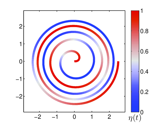
Figure 3: The distribution for $A=5$ and $\omega=3$.

We ran simulations with a twofold purpose: (a) to ascertain the convergence of various classifier risks to the Bayes optimal risk and to compare their rates of convergence and (b) to compare the actual runtimes of the various algorithms. To this end, we took $\mathcal{X}=\mathbb{R}^{2}$ endowed with the Euclidean metric $\rho(x,x^{\prime})=\|x-x^{\prime}\|_{2}$, and defined a joint distribution over $\mathcal{X}\times\{-1,1\}$ as follows. A point $(x_{1},x_{2})\in\mathbb{R}^{2}$ is sampled by drawing $T\in[0,2\pi]$ uniformly at random and putting

$$x_{1}(T) = A\sqrt{T}\cos(\omega T),$$

$$x_{2}(T) = A\sqrt{T}\sin(\omega T)$$

for some specified parameters $A$ and $\omega$. The label $Y\in\{-1,1\}$ is drawn according to the conditional distribution

$$\eta(T)=\mathbb{P}(Y=1\,|\,T)=\frac{1+\cos(\omega T)}{2},$$

as illustrated in Figure 3.

We compared four classifiers: $k^{*}$-NN (the $k$-NN classifier with $k$ optimized by cross-validation), SVM (support vector machine with the RBF kernel whose bandwidth and regularization penalty were optimized by cross-validation), CV-1-NN (margin-regularized 1-NN with $\gamma$ tuned by cross-validation), and SRM-1-NN (the 1-NN classifier described in Section 3 using a greedy vertex cover heuristic rather than the exact matching algorithm while searching for the optimal margin). Their runtime and generalization performance, averaged over $100$ independent runs, are summarized in Figures 4 and 5.

Our proposed algorithm, SRM-1-NN, emerges competitive by both criteria.

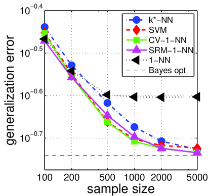
Figure 4: Generalization error vs. number of samples. CV-1-NN is uniformly dominant, but for large sample sizes SRM-1-NN catches up. Unregularized $1$-NN is included for reference; it is clearly not Bayes consistent.

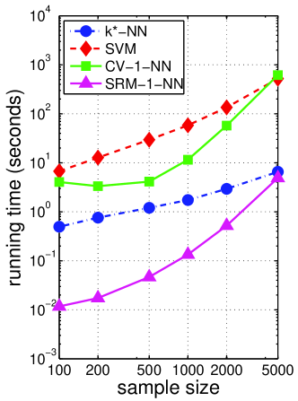
Figure 5: Running time vs. number of samples. SRM-1-NN enjoys a clear time advantage over the other methods involving cross-validation.

Appendix A Appendix

A.1 Proof of Lemma 3

We first need the following uniform convergence lemma.

Lemma 7.

For any $0<\varepsilon$, $0<\xi<1$ and $0<\gamma$,

$$\mathbb{P}\Big{(}\sup_{f\in\mathcal{F}_{2}}\left|\mathcal{L}_{\gamma,\xi}(f)-\widehat{\mathcal{L}}_{n,\gamma,\xi}(f)\right|$$ (24)

$$\hskip 40.0pt>2\mathcal{R}_{n}(\mathcal{L}_{\gamma,\xi}\circ\mathcal{F}_{2})+\varepsilon\Big{)}\leq\exp\left(-n\varepsilon^{2}/c_{1}\right),$$

where the Rademacher complexity $\mathcal{R}_{n}(\mathcal{L}_{\gamma,\xi}\circ\mathcal{F}_{2})$ satisfies

$$\mathcal{R}_{n}(\mathcal{L}_{\gamma,\xi}\circ\mathcal{F}_{2})\,\leq\,\frac{2}{\gamma\xi}\left(\frac{c_{d}}{n}\right)^{\frac{1}{d+1}}\;=:\;\mathcal{R}_{n,\gamma,\xi}.$$ (25)

Proof of Lemma 7.

Equation (24) is restatement of Mohri et al. (2012, Theorem 3.1). Note that $\Phi_{\gamma,\xi}:\mathbb{R}\to[0,1]$ is ${1/(\gamma\xi)}$-Lipschitz. Thus, by Talagrand’s contraction lemma (Ledoux and Talagrand, 1991),

$$\mathcal{R}_{n}(\mathcal{L}_{\gamma,\xi}\circ\mathcal{F}_{2})\leq\frac{2}{\gamma\xi}\mathcal{R}_{n}({\mathcal{F}_{1}}).$$

The upper estimate on $\mathcal{R}_{n}({\mathcal{F}_{1}})$ implicit in (25) is essentially contained in Equation (10) of Kontorovich and Weiss (2014). ∎

Proof of Lemma 3.

Following proof idea in Devroye et al. (1996, Theorem 18.2), a union bound yields

$$\mbox{(***)}\;:=\; \mathbb{P}\Big{(}\exists l\in\mathbb{N}:\sup_{f\in\mathcal{F}_{2}}\Big{|}{\mathcal{L}_{\gamma_{n,l},\xi_{n}}(f)-\widehat{\mathcal{L}}_{n,\gamma_{n,l},\xi_{n}}(f)}\Big{|}$$

$$\hskip 10.0pt>\varepsilon+\varepsilon_{n,l}\Big{)}$$

$$\;\leq\; \sum_{l=1}^{\infty}\mathbb{P}\Big{(}\sup_{f\in\mathcal{F}_{2}}\Big{|}{\mathcal{L}_{\gamma_{n,l},\xi_{n}}(f)-\widehat{\mathcal{L}}_{n,\gamma_{n,l},\xi_{n}}(f)}\Big{|}$$

$$\hskip 10.0pt>\varepsilon+\varepsilon_{n,l}\Big{)}.$$

Note that by construction

$$\varepsilon_{n,l} = 2\mathcal{R}_{n,\gamma_{n,l},\xi_{n}}+\sqrt{\!\frac{{2c_{1}}\log\left(\frac{1}{\xi_{n}}\log\frac{e}{\gamma_{n,l}}\right)}{n}}\!.$$

Thus, writing

$$r_{n,l}=\sqrt{\!\frac{{2c_{1}}\log\left(\frac{1}{\xi_{n}}\log\frac{e}{\gamma_{n,l}}\right)}{n}}\!$$

and bounding each term in the sum by Lemma 7, we have

(***) $$\leq \sum_{l=1}^{\infty}\exp\left(-\frac{n(\varepsilon+r_{n,l})^{2}}{c_{1}}\right)$$

$$\leq \exp\left(-\frac{n\varepsilon^{2}}{c_{1}}\right)\sum_{l=1}^{\infty}\exp\left(-\frac{nr_{n,l}^{2}}{c_{1}}\right).$$

Next note that by the definition of $\gamma_{n,l}$ we have

$$\gamma_{n,l}=(1-\xi_{n})^{l-1}\leq\exp\left(-\xi_{n}(l-1)\right).$$

Solving for $l$ yields

$$\frac{1}{\xi_{n}}\log\frac{e}{\gamma_{n,l}}\geq l.$$

Thus,

$$\exp\left(-\frac{nr_{n,l}^{2}}{c_{1}}\right) \leq \frac{1}{l^{2}}$$

and summing over $l$ yields the claim. ∎

A.2 Proof of Lemma 4

Let us first write $\varepsilon_{n,l}$ in terms of $\gamma_{n,l-1}$. Since $\gamma_{n,l}=\gamma_{n,l-1}(1-\xi_{n})$ by definition, we have

$$\varepsilon_{n,l} = \frac{2}{\gamma_{n,l-1}(1-\xi_{n})\xi_{n}n_{d}^{2}}$$

$$+\sqrt{\frac{{2c_{1}}{}\log\left(\frac{1}{\xi_{n}}\log\frac{e}{\gamma_{n,l-1}(1-\xi_{n})}\right)}{n}}.$$

Taking $n$ sufficiently large to ensure that $1-\xi_{n}\geq 1/2$ we have that for all $l\geq 2$,

$$\varepsilon_{n,l}\leq\frac{4}{\gamma_{n,l-1}\xi_{n}n_{d}^{2}}+\sqrt{\!\frac{{2c_{1}}{}\log\left(\frac{1}{\xi_{n}}\log\frac{2e}{\gamma_{n,l-1}}\right)}{n}}\!,$$

which is exactly $r^{\textrm{{\tiny{PEN}}}}(n,\gamma_{n,l-1})$.

A.3 Proof of Lemma 5

The function $\eta:\mathcal{X}\to[0,1]$ given by $\eta(x)=\mathbb{P}(Y=1|X=x)$ is measurable (Schervish, 1995, Corollary B.22) and hence, by virtue of being bounded, belongs to $L_{1}(\mu)$, where $\mu$ is the marginal distribution over $\mathcal{X}$.

Now

$$R^{*} = \mathbb{P}(Y(\eta(X)-{\textstyle\frac{1}{2}})\leq 0)$$

$$= \lim_{k\to\infty}\mathbb{P}\left(Y(\eta(X)-{\textstyle\frac{1}{2}})<1/k\right)$$

$$= \lim_{k\to\infty}\mathbb{P}\left(kY(\eta(X)-{\textstyle\frac{1}{2}})<1\right)$$

$$= \lim_{k\to\infty}\mathbb{P}(g_{k}(X,Y)<1),$$

where $g_{k}(x,y):=ky(\eta(x)-{\textstyle\frac{1}{2}})\in L_{1}(\mu)$ and we invoked Lebesgue’s dominated convergence theorem together with the fact that $\mathds{1}[\alpha<\frac{1}{k}]\mathop{\longrightarrow}\limits_{k\to\infty}\mathds{1}[\alpha\leq 0]$ for all $\alpha\in\mathbb{R}$.

We also observe that $R_{\gamma}(f)=\mathbb{P}(Yf(X)<\gamma)=r$ for some $f\in\mathcal{F}_{2}$ if and only if there is an $\tilde{f}\in\mathcal{F}_{2/\gamma}$ for which $r=\mathbb{P}(Y\tilde{f}(X)<1)$. Define the metric $\tilde{\rho}$ on $\mathcal{X}\times\mathcal{Y}$ by $\tilde{\rho}((x,y),(x^{\prime},y^{\prime}))=\rho(x,x^{\prime})+\mathds{1}[y\neq y^{\prime}]$ and denote the collection of all $L$-Lipschitz functions on $(\mathcal{X}\times\mathcal{Y},\tilde{\rho})$ by $\tilde{\mathcal{F}}_{L}$. The compactness of $(\mathcal{X}\times\mathcal{Y},\tilde{\rho})$ is inherited from $(\mathcal{X},\rho)$ and each $f\in\bigcup_{L\geq 0}\mathcal{F}_{L}$ has $\left\|f\right\|_{\infty}<\infty$. Since for $f\in\mathcal{F}_{L}$,

$$yf(x)-y^{\prime}f(x^{\prime}) = yf(x)-yf(x^{\prime})+yf(x^{\prime})-y^{\prime}f(x^{\prime})$$

$$\leq \left|f(x)-f(x^{\prime})\right|+2\left\|f\right\|_{\infty}\mathds{1}[y\neq y^{\prime}]$$

$$\leq \max\left\{L,2\left\|f\right\|_{\infty}\right\}\tilde{\rho}((x,y),(x^{\prime},y^{\prime})),$$

and conversely, for $yf(\cdot)\in\tilde{\mathcal{F}}_{L}$,

$$|f(x)-f(x^{\prime})|=|yf(x)-yf(x^{\prime})|\leq L,$$

it follows that $f\in\bigcup_{L\geq 0}\mathcal{F}_{L}$ if and only if $yf(\cdot)\in\bigcup_{L\geq 0}\tilde{\mathcal{F}}_{L}$.

We claim that the collection of all Lipschitz functions, $\bigcup_{L\geq 0}\tilde{\mathcal{F}}_{L}$ is dense in $L_{1}(\mu)$. Indeed, Theorem 8 below shows that the continuous functions are dense in $L_{1}(\mu)$, and these can be uniformly approximated by Lipschitz ones in our case Georganopoulos (1967); Miculescu (2000). In particular, given our assumptions on $\mathcal{X}$ and $\mu$, it follows that for all $g\in L_{1}(\mu)$ and all $\varepsilon>0$ there is an $\tilde{f}\in\bigcup_{L\geq 0}\tilde{\mathcal{F}}_{L}$ such that $\left\|\tilde{f}-g\right\|_{\infty}<\varepsilon$.

In particular, for each $g_{k}$ there is a sequence $(f_{k,\ell})_{\ell\in\mathbb{N}}\subset\bigcup_{L\geq 0}\tilde{\mathcal{F}}_{L}$ such that $f_{k,\ell}(x,y)\mathop{\longrightarrow}\limits_{\ell\to\infty}g_{k}(x,y)$ almost everywhere $[\mu]$. Also, $a_{n}\mathop{\longrightarrow}\limits_{n\to\infty}a$ implies

$$\mathds{1}[a_{n}<1]\mathop{\longrightarrow}\limits_{n\to\infty}\mathds{1}[a<1].$$

Applying Lebesgue’s dominated convergence theorem again,

$$\mathbb{P}(g_{k}(X,Y)<1) = \lim_{\ell\to\infty}\mathbb{P}(f_{k,\ell}(X,Y)<1).$$

It follows that

$$R^{*}=\lim_{k\to\infty}\lim_{\ell\to\infty}\mathbb{P}(f_{k,\ell}(X,Y)<1),$$

which proves the claim.

A.4 Proof of Lemma 6

Rescaling $f\in\mathcal{F}_{2}$ to $g=2f/\gamma$, Eq. (23) is equivalent to claiming the existence of an $n_{0}({\varepsilon})\in\mathbb{N}$ such that for all $n\geq n_{0}(\varepsilon)$,

$$\left|\mathcal{L}_{1,\xi_{n}}(g)-R_{1}(g)\right| \leq \varepsilon/4.$$

Since ${\xi_{n}=n_{d}^{-1}}$ decays to zero with increasing $n$, it follows that $\mathcal{L}_{1,n_{d}^{-1}}(g)\mathop{\longrightarrow}\limits_{n\to\infty}R_{1}(g)$ pointwise, and so by Lebesgue’s dominated convergence theorem, we have that

$$\lim_{n\to\infty}\mathcal{L}_{1,{n_{d}^{-1}}}(g)=R_{1}(g),$$

proving the claim.

Background on metric measure spaces

Here we provide some general relevant background on metric measure spaces. Our metric space $(\mathcal{X},\rho)$ is doubling, but in this section finite diameter is not assumed. We recall some standard definitions. A topological space is Hausdorff if every two distinct points have disjoint neighborhoods. It is a standard (and obvious) fact that all metric spaces are Hausdorff.

A metric space $\mathcal{X}$ is complete if every Cauchy sequence converges to a point in $\mathcal{X}$. Every metric space may be completed by (essentially) adjoining to it the limits of all of its Cauchy sequences (Rudin, 1976, Exercise 3.24); moreover, the completion is unique up to isometry (Munkres, 1975, Section 43, Exercise 10). We implicitly assume throughout the paper that $\mathcal{X}$ is complete. Closed subsets of complete metric spaces are also complete metric spaces under the inherited metric.

A topological space $\mathcal{X}$ is locally compact if every point $x\in\mathcal{X}$ has a compact neighborhood. It is a standard and easy fact that complete doubling spaces are locally compact. Indeed, consider any $x\in\mathcal{X}$ and the open $r$-ball about $x$, $B_{r}(x):=\left\{y\in\mathcal{X}:\rho(x,y)<r\right\}$. We must show that $\operatorname{cl}(B_{r}(x))$ — the closure of $B_{r}(x)$ — is compact. To this end, it suffices to show that $\operatorname{cl}(B_{r}(x))$ is totally bounded (that is, has a finite $\varepsilon$-covering number for each $\varepsilon>0$), since in complete metric spaces, a set is compact iff it is closed and totally bounded (Munkres, 1975, Theorem 45.1). Total boundedness follows immediately from the doubling property. The latter posits a constant $k$ and some $x_{1},\ldots,x_{k}\in\mathcal{X}$ such that $B_{r}(x)\subseteq\cup_{i=1}^{k}B_{r/2}(x_{i})$. Then certainly $\operatorname{cl}(B_{r}(x))\subseteq\cup_{i=1}^{k}B_{2r/3}(x_{i}).$ We now apply the doubling property recursively to each of the $B_{2r/3}(x_{i})$, until the radius of the covering balls becomes smaller than $\varepsilon$.

We now recall some standard facts from measure theory. Any topology on $\mathcal{X}$ (and in particular, the one induced by the metric $\rho$), induces the Borel $\sigma$-algebra $\mathscr{B}$. A Borel probability measure is a function $\mu:\mathscr{B}\to[0,1]$ that is countably additive and normalized by $\mu(\mathcal{X})=1$. The latter is complete if for all $A\subseteq B\in\mathscr{B}$ for which $\mu(B)=0$, we also have $\mu(A)=0$. Any Borel $\sigma$-algebra may be completed by defining the measure of any subset of a measure-zero set to be zero (Rudin, 1987, Theorem 1.36). We implicitly assume throughout the paper that $(\mathcal{X},\mathscr{A},\mu)$ is a complete measure space, where $\mathscr{A}$ contains all of the Borel sets.

The measure $\mu$ is said to be outer regular if it can be approximated from above by open sets: For every $E\in\mathscr{A}$, we have

$$\mu(E)=\inf\left\{\mu(V):E\subseteq V,V~{}\text{open}\right\}.$$

A corresponding inner regularity corresponds to approximability from below by compact sets: For every $E\in\mathscr{A}$,

$$\mu(E)=\sup\left\{\mu(K):K\subseteq E,K~{}\text{compact}\right\}.$$

The measure $\mu$ is regular if it is both inner and outer regular. Any probability measure defined on the Borel $\sigma$-algebra of a metric space is regular (Kallenberg, 2002, Lemma 1.19). (Dropping the “metric” or “probability” assumptions opens the door to various exotic pathologies (Bogachev, 2007, Chapter 7), (Rudin, 1987, Exercise 2.17).)

Finally, we have the following technical result, adapted from (Rudin, 1987, Theorem 3.14) to our setting:

Theorem 8.

Let $\mathcal{X}$ be a complete doubling metric space equipped with a complete probability measure $\mu$, such that all Borel sets are $\mu$-measurable. Then $C_{c}(\mathcal{X})$ (the collection of continuous functions with compact support) is dense in $L_{1}(\mu)$.

References

- Weinberger and Saul (2009) Kilian Q Weinberger and Lawrence K Saul. Distance metric learning for large margin nearest neighbor classification. Journal of Machine Learning Research, 10(Feb):207–244, 2009.
- Boiman et al. (2008) Oren Boiman, Eli Shechtman, and Michal Irani. In defense of nearest-neighbor based image classification. In 2008 IEEE Computer Society Conference on Computer Vision and Pattern Recognition (CVPR 2008), 24-26 June 2008, Anchorage, Alaska, USA, 2008. doi: 10.1109/CVPR.2008.4587598. URL https://doi.org/10.1109/CVPR.2008.4587598.
- Cover and Hart (1967) T. M. Cover and P. E. Hart. Nearest neighbor pattern classification. IEEE Transactions on Information Theory, 13:21–27, 1967.
- Stone (1977) Charles J Stone. Consistent nonparametric regression. The annals of statistics, pages 595–620, 1977.
- Devroye and Gyorfi (1985) L. Devroye and L. Gyorfi. Nonparametric Density Estimation: The L1 View. Wiley Interscience Series in Discrete Mathematics. Wiley, 1985. ISBN 9780471816461. URL https://books.google.co.il/books?id=ZVALbrjGpCoC.
- Zhao (1985) Lin Cheng Zhao. Exponential bounds of mean error for the nearest neighbor estimates of regression functions. Technical report, PITTSBURGH UNIV PA CENTER FOR MULTIVARIATE ANALYSIS, 1985.
- Hart (1968) Peter Hart. The condensed nearest neighbor rule (corresp.). IEEE transactions on information theory, 14(3):515–516, 1968.
- Gates (1972) Geoffrey Gates. The reduced nearest neighbor rule (corresp.). IEEE transactions on information theory, 18(3):431–433, 1972.
- Ritter et al. (1975) G Ritter, H Woodruff, S Lowry, and T Isenhour. An algorithm for a selective nearest neighbor decision rule (corresp.). IEEE Transactions on Information Theory, 21(6):665–669, 1975.
- Wilson and Martinez (2000) D Randall Wilson and Tony R Martinez. Reduction techniques for instance-based learning algorithms. Machine learning, 38(3):257–286, 2000.
- Gottlieb et al. (2018) Lee-Ad Gottlieb, Aryeh Kontorovich, and Pinhas Nisnevitch. Near-optimal sample compression for nearest neighbors. IEEE Transactions on Information Theory, 64(6):4120–4128, 2018.
- Krauthgamer and Lee (2004) R. Krauthgamer and J. R. Lee. Navigating nets: Simple algorithms for proximity search. In 15th Annual ACM-SIAM Symposium on Discrete Algorithms, pages 791–801, January 2004.
- Beygelzimer et al. (2006) Alina Beygelzimer, Sham Kakade, and John Langford. Cover trees for nearest neighbor. In Proceedings of the 23rd international conference on Machine learning, pages 97–104. ACM, 2006.
- Andoni and Indyk (2006) Alexandr Andoni and Piotr Indyk. Near-optimal hashing algorithms for approximate nearest neighbor in high dimensions. In Foundations of Computer Science, 2006. FOCS’06. 47th Annual IEEE Symposium on, pages 459–468. IEEE, 2006.
- Gottlieb et al. (2010) Lee-Ad Gottlieb, Leonid Kontorovich, and Robert Krauthgamer. Efficient classification for metric data. In COLT, pages 433–440, 2010.
- von Luxburg and Bousquet (2004) Ulrike von Luxburg and Olivier Bousquet. Distance-based classification with lipschitz functions. Journal of Machine Learning Research, 5:669–695, 2004.
- Devroye et al. (1996) Luc Devroye, László Györfi, and Gábor Lugosi. A probabilistic theory of pattern recognition, volume 31 of Applications of Mathematics (New York). Springer-Verlag, New York, 1996. ISBN 0-387-94618-7.
- Shalev-Shwartz and Ben-David (2014) Shai Shalev-Shwartz and Shai Ben-David. Understanding Machine Learning: From Theory to Algorithms. Cambridge University Press, New York, NY, USA, 2014. ISBN 1107057132, 9781107057135.
- Chaudhuri and Dasgupta (2014) Kamalika Chaudhuri and Sanjoy Dasgupta. Rates of convergence for nearest neighbor classification. In Advances in Neural Information Processing Systems, pages 3437–3445, 2014.
- Snapp et al. (1998) Robert R Snapp, Santosh S Venkatesh, et al. Asymptotic expansions of the nearest neighbor risk. The Annals of Statistics, 26(3):850–878, 1998.
- Psaltis et al. (1994) Demetri Psaltis, R Snapp, and Santosh S Venkatesh. On the finite sample performance of the nearest neighbor classifier. IEEE Transactions on Information Theory, 40(3):820–837, 1994.
- Littlestone and Warmuth (1986) Nick Littlestone and Manfred K. Warmuth. Relating data compression and learnability, unpublished. 1986.
- Graepel et al. (2005) Thore Graepel, Ralf Herbrich, and John Shawe-Taylor. Pac-bayesian compression bounds on the prediction error of learning algorithms for classification. Machine Learning, 59(1-2):55–76, 2005.
- Mohri et al. (2012) Mehryar Mohri, Afshin Rostamizadeh, and Ameet Talwalkar. Foundations of machine learning. MIT press, 2012.
- Mucha and Sankowski (2004) Marcin Mucha and Piotr Sankowski. Maximum matchings via gaussian elimination. In FOCS ’04: Proceedings of the 45th Annual IEEE Symposium on Foundations of Computer Science, pages 248–255, Washington, DC, USA, 2004. IEEE Computer Society. ISBN 0-7695-2228-9. doi: http://dx.doi.org/10.1109/FOCS.2004.40.
- Gottlieb et al. (2014) Lee-Ad Gottlieb, Aryeh Kontorovich, and Robert Krauthgamer. Efficient classification for metric data. IEEE Transactions on Information Theory, 60(9):5750–5759, 2014.
- Ledoux and Talagrand (1991) Michel Ledoux and Michel Talagrand. Probability in Banach Spaces. Springer-Verlag, 1991.
- Kontorovich and Weiss (2014) Aryeh Kontorovich and Roi Weiss. Maximum margin multiclass nearest neighbors. In International Conference on Machine Learning, pages 892–900, 2014.
- Schervish (1995) Mark J. Schervish. Theory of statistics. Springer Series in Statistics. Springer-Verlag, New York, 1995. ISBN 0-387-94546-6. doi: 10.1007/978-1-4612-4250-5. URL https://doi.org/10.1007/978-1-4612-4250-5.
- Georganopoulos (1967) Georgios Georganopoulos. Sur l’approximation des fonctions continues par des fonctions lipschitziennes. C. R. Acad. Sci. Paris Sér. A-B, 264:A319–A321, 1967.
- Miculescu (2000) Radu Miculescu. Approximation of continuous functions by lipschitz functions. Real Anal. Exchange, 26(1):449–452, 2000. URL https://projecteuclid.org:443/euclid.rae/1230939175.
- Rudin (1976) Walter Rudin. Principles of mathematical analysis. McGraw-Hill Book Co., New York, third edition, 1976. International Series in Pure and Applied Mathematics.
- Munkres (1975) James R. Munkres. Topology: a first course. Prentice-Hall, Inc., Englewood Cliffs, N.J., 1975.
- Rudin (1987) Walter Rudin. Real and Complex Analysis. McGraw-Hill, 1987.
- Kallenberg (2002) Olav Kallenberg. Foundations of modern probability. Second edition. Probability and its Applications. Springer-Verlag, 2002.
- Bogachev (2007) V. I. Bogachev. Measure theory. Vol. I, II. Springer-Verlag, Berlin, 2007. ISBN 978-3-540-34513-8; 3-540-34513-2. doi: 10.1007/978-3-540-34514-5. URL http://dx.doi.org/10.1007/978-3-540-34514-5.