Solving the inverse problem of noise-driven dynamic networks

Abstract

Nowadays massive amount of data are available for analysis in natural and social systems. Inferring system structures from the data, i.e., the inverse problem, has become one of the central issues in many disciplines and interdisciplinary studies. In this Letter, we study the inverse problem of stochastic dynamic complex networks. We derive analytically a simple and universal inference formula called double correlation matrix (DCM) method. Numerical simulations confirm that the DCM method can accurately depict both network structures and noise correlations by using available kinetic data only. This inference performance was never regarded possible by theoretical derivation, numerical computation and experimental design.

Introduction. In recent decades, large scale of data sets have been accumulated in various and wide fields, in particular in social and biological systems  Butte et al. (2000); Kim et al. (2001); Bar-Joseph et al. (2003, 2012). There are massive amount of data available for utilization, however, the system structures yielding these data are often not clear Feist et al. (2009); De Smet and Marchal (2010). Therefore, deducing the connectivity of systems from these data, i.e., the inverse problem, turns to be today one of the central issues in interdisciplinary fields Yeung et al. (2002); Stuart et al. (2003); Segal et al. (2003); Hu et al. (2007); Lezon et al. (2006); Barzel and Barabasi (2013); Feizi et al. (2013). A typical example of inference efforts is a recent project of the Dialogue on Reverse Engineering Assessment and Methods (DREAM) which has attracted extensive attention for reconstructing gene regulatory networks from high-throughput microarray data Marbach et al. (2010, 2012). Similar goals have been also pursued in other fields, such as neural networks Bullmore and Sporns (2009), ecosystems Sugihara et al. (2012), chemical reactions Arkin and Ross (1995); Arkin et al. (1997) and so on. Most of biological and social systems contain many units which evolve collectively with very complicated interaction structures represented by complex networks Watts and Strogatz (1998); Barabasi and Albert (1999); Barabasi and Oltvai (2004). Mathematically, the dynamics of these complex systems are extensively described by sets of coupled ordinary differential equations (ODEs) Glass and Mackey (1988); Goldbeter (1996); Alon (2007); Tsai et al. (2008). The inverse problems of these systems can thus be interpreted as to retrieve the interaction Jacobian matrices from the measurable data of dynamical variables of networks. So far, a wide range of network inference methods have been proposed to address this issue in diverse fields. Available methods can be classified into several broad categories Basso et al. (2005); Bansal et al. (2007); Marbach et al. (2012); Villaverde et al. (2013): Bayesian networks and probabilistic graphical models, which maximize a scoring function over alternative network models Jansen et al. (2003); Friedman (2004); regression techniques, which fit the data to a priori models  Haury et al. (2012); integrative bioinformatics approaches, which combine data from a number of independent experimental clues Gardner et al. (2003); Covert et al. (2004); statistical methods, which rely on a variety of measures of pairwise correlations or mutual information and other methods Eisen et al. (1998); Basso et al. (2005); Faith et al. (2007).

The complexity of networks can hinder the attempt to solve the inverse problems Gardner et al. (2003). Moreover, the network dynamics are inevitably perturbed by many uncontrollable impacts, called noise, and these random and unknown perturbations make the inverse problems even more difficult. Actually, noise can play two seemingly contradictory effects. On one hand noise can contaminate data, mask noise-free network dynamics and thus lead to inference errors. On the other hand, noise perturbations are helpful to provide rich distinctive data which involve useful information for effective inferences, as emphasized recently by Ren et al. (2010). However, the latter role of noise has been ignored by most of current inference methods. The results of the currently prevailing inference methods are thus unsatisfactory, in particular if noise is unknown and noise effect plays crucial role in data productions. To overcome these difficulties, new comprehensive physical ideas and intelligent mathematical methods become absolutely necessary.

In the present work, a novel double correlation matrix (DCM) method is proposed to generally solve the inverse problems of dynamic complex networks driven by noise, and we derive a compact and universal algorithm $\hat{\mathbf{A}}=\hat{\mathbf{B}}\hat{\mathbf{C}}^{-1}$ with $\hat{\mathbf{A}}$ being the target of the inverse problems, i.e., the interaction Jacobian matrix, $\hat{\mathbf{C}}$ the variable-variable correlation matrix and $\hat{\mathbf{B}}$ the velocity-variable correlation matrix. All elements in $\hat{\mathbf{B}}$ and $\hat{\mathbf{C}}$ can be explicitly computed from the measurable variable data only.

In contrast with all the previous methods, the DCM method has two remarkable advantages. First, it extracts more useful information from the available data by computing double correlation matrices $\hat{\mathbf{B}}$ and $\hat{\mathbf{C}}$ while only a single matrix has been considered in most of inference methods Levnaji and Pikovsky (2014). Second, it effectively filters out noise contamination without requiring detailed correlation statistics of noise by using the fast varying property of noise. This property is available for most of practical systems while, to our knowledge, has never been fully utilized so far in inverse computations. Due to these advantages, the DCM method can infer the structure of noise-driven dynamic networks incomparably more effectively and accurately than currently prevailing inference methods do.

Theory. A large class of dynamic networks can be most generally represented by the following coupled ODEs driven by noise

$$\dot{\mathbf{x}}(t)=\mathbf{f}(\mathbf{x}(t),\eta(t)),$$ (1)

with variables ${\mathbf{x}(t)=(x_{1}(t),x_{2}(t),\cdots,x_{N}(t))}$, noise ${\mathbf{\eta}(t)=(\eta_{1}(t),\eta_{2}(t),\cdots,\eta_{M}(t))}$ and dynamic fields ${\mathbf{f}(\mathbf{x}(t),\eta(t))=(f_{1}(\mathbf{x}(t),\eta(t)),\cdots,f_{N}(\mathbf{x}(t),\eta(t)))}$. In this Letter, we adopt white noise approximation for very short noise correlation time,

$$\langle{\eta_{i}(t)}\rangle=0,{\langle{\eta_{i}(t)\eta_{j}(t^{\prime})}\rangle}=D_{ij}\delta(t-t^{\prime}),{i,j=1,2,\cdots,M}.$$

In most of realistic systems, this approximation does be valid when noise serves as perturbations from microscopic world varying much faster than the macroscopic variables. Around any phase space point $\mathbf{x}$ and for small noise approximation, Eq. (1) can be linearized to

$$\dot{\mathbf{y}}(t)=\hat{\mathbf{A}}(\mathbf{x})\mathbf{y}(t)+\Gamma(t),$$ (2)

$${{\mathbf{y}}(t)=(y_{1}(t),\cdots,y_{N}(t))},{\Gamma(t)=(\Gamma_{1}(t),\cdots,\Gamma_{N}(t))},$$

$${\langle{\Gamma(t)}\rangle=0},{\langle{\Gamma_{i}(t)\Gamma_{j}(t^{\prime})}\rangle=Q_{ij}\delta(t-t^{\prime})}.$$ (3)

where ${\mathbf{y}(t)=\mathbf{x}(t)-\mathbf{x}},$ ${A_{ij}(\mathbf{x})=\frac{\partial{f_{i}}}{\partial{x_{j}}}\mid_{\mathbf{x}(t)=\mathbf{x},\eta(t)=0}},$ $\Gamma_{i}(t)={\sum_{\mu=1}^{M}}G_{i{\mu}}{\eta_{\mu}},$ ${G_{i\mu}=\frac{\partial{f_{i}}}{\partial{\eta_{\mu}}}\mid_{\mathbf{x}(t)=\mathbf{x},\eta(t)=0}}$ and ${Q_{ij}={\sum_{\mu=1}^{M}}{\sum_{\nu=1}^{M}}G_{i\mu}D_{\mu{\nu}}G_{\nu{j}}^{T}}.$

Without noise ($\eta(t)=0$) Eq. (1) evolves to one of their attractors over time which may be a stable steady state, a periodic or chaotic state. In any case, the dimension of the attractor $d_{a}$ should be considerably smaller than that of the original network $d_{a}\ll{N}$. Therefore, it is impossible to use the data set of an attractor of noise-free system to infer the network structure due to lack of sufficient information in the data. Existence of noise can scatter the variable data to fill $N$-dimensional phase space and provide possibility (sufficient information) to identify the full interactions of the network.

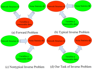
Figure 1: (Color online) Schematic figures on forward and inverse problems of complex networks of Eq. (2). (a) Forward problem of Eq. (2): From network structure $\hat{\mathbf{A}}$ and noise statistics $\hat{\mathbf{Q}}$ to calculate output variable data $\mathbf{y}(t)$. (b) Typical inverse problem: From available output variable data $\mathbf{y}(t)$ and noise statistics $\hat{\mathbf{Q}}$ to retrieve network Jacobian structure $\hat{\mathbf{A}}$, by using matrix equation $\hat{\mathbf{A}}\hat{\mathbf{C}}+\hat{\mathbf{C}}\hat{\mathbf{A}}^{T}=-\hat{\mathbf{Q}}$ Ren et al. (2010); Ching et al. (2013); Risken (1984) with $\hat{\mathbf{A}}$, $\hat{\mathbf{Q}}$ and $\hat{\mathbf{C}}$ given in Eqs. (2)(3)(7). (c) Another nontypical inverse problem: From available variable data $\mathbf{y}(t)$ and Jacobian structure $\hat{\mathbf{A}}$ to depict noise statistics $\hat{\mathbf{Q}}$. (d) A desirable inverse computational target not regarded possible so far: From available variable data $\mathbf{y}(t)$ only to reveal both network Jacobian structure $\hat{\mathbf{A}}$ and noise statistics $\hat{\mathbf{Q}}$. And this is the task of this Letter.

With both linearized matrix $\hat{\mathbf{A}}$ in (2) and noise statistics $\hat{\mathbf{Q}}$ in (3) given, we can calculate output variables $\mathbf{y}(t)$ as a well known forward problem of dynamic networks (Fig. 1(a)). A typical inverse problem is to retrieve the interaction Jacobian matrix $\hat{\mathbf{A}}$ with measurable output data $\mathbf{y}(t)$ and known noise statistics $\hat{\mathbf{Q}}$ (Fig. 1(b)) Ren et al. (2010); Risken (1984). This inverse problem can be solved for certain simple symmetric network structures, whereas it is not solvable in many complicated cases, such as when networks have asymmetric links or when the basic noise-free networks have nonsteady and nonsynchronous motions Ching et al. (2013); Wang et al. (2009); Ren et al. (2010). Another trivial and nontypical inverse problem is to reveal noise statistics $\hat{\mathbf{Q}}$ with known output data $\mathbf{y}(t)$ and network structures $\hat{\mathbf{A}}$ (Fig. 1(c)). However, the inference condition of Fig. 1(b) is not reasonable in practice. Since noise represents some random and uncontrollable factors, even less information can be obtained on noise than on network structures and it is unreasonable to have known knowledge of noise statistics $\hat{\mathbf{Q}}$ to infer unknown network structure $\hat{\mathbf{A}}$. A most effective as well as most desirable inverse target is presented in Fig. 1(d) where one can solve the inverse problem merely from the measurable data $\mathbf{y}(t)$ with both network structures $\hat{\mathbf{A}}$ and noise statistics $\hat{\mathbf{Q}}$ unknown. This inference performance has never been regarded possible so far by theoretical analysis and experimental design. And this is right the issue discussed in this Letter.

Now, we consider how to infer network structure $\hat{\mathbf{A}}$ merely from measurable data $\mathbf{y}(t)$. Suppose we have $L$ pairs of variable data ($\mathbf{x}(t_{q}),\mathbf{x}(t_{q}+\Delta{t_{q}}),{q=1,2,\cdots,L}$) in a small phase space region, with all $\Delta{t_{q}}$, $\|\mathbf{x}(t_{q^{\prime}})-\mathbf{x}(t_{q})\|$, $\|\mathbf{x}(t_{q^{\prime}}+\Delta{t_{q^{\prime}}})-\mathbf{x}(t_{q})\|$ $\ll{1}$ for all $q$, $q^{\prime}$. From the available data we can extract full information of $\mathbf{y}(t_{q})=\mathbf{x}(t_{q})-\mathbf{x}$ and $\mathbf{x}=\frac{1}{L}\sum_{q=1}^{L}{\mathbf{x}(t_{q})}$. The velocity term $\dot{\mathbf{y}}(t_{q})$ in Eq. (2) can be measured as

$$\dot{y}_{i}(t_{q})=\frac{y_{i}(t_{q}+\Delta{t_{q}})-y_{i}(t_{q})}{\Delta{t_{q}}}.$$ (4)

With all the quantities ${\mathbf{y}}(t_{q})$ and $\dot{\mathbf{y}}(t_{q})$ measured, we can derive some explicit and compact algorithms from Eq. (2) as

$$\hat{\mathbf{A}}=\hat{\mathbf{B}}\hat{\mathbf{C}}^{-1},$$ (5)

and

$$\hat{\mathbf{Q}}=-2\hat{\mathbf{B}}_{s}=-(\hat{\mathbf{B}}+\hat{\mathbf{B}}^{T}),$$ (6)

where $\hat{\mathbf{C}}=\langle{{\mathbf{y}}\mathbf{y}^{T}}\rangle$ and $\hat{\mathbf{B}}=\langle{\dot{\mathbf{y}}\mathbf{y}^{T}}\rangle$ are the variable-variable and velocity-variable correlation matrices, respectively,

$$C_{ij}={\frac{1}{L}}{\sum_{q=1}^{L}}y_{i}(t_{q})y_{j}(t_{q}),B_{ij}={\frac{1}{L}}{\sum_{q=1}^{L}}\dot{y}_{i}(t_{q})y_{j}(t_{q}).$$ (7)

And $\hat{\mathbf{B}}_{s}$ and $\hat{\mathbf{B}}^{T}$ are the symmetric part and the transposition of $\hat{\mathbf{B}}$, respectively. The detailed derivations of (5) and (6) are given in Supplemental Material SM I.

Now, a novel double correlation matrix (DCM) method is proposed to generally solve the inverse problem of Eq. (2) and also explicitly depict noise statistical correlation matrix $\hat{\mathbf{Q}}$, by using the simple and unified algorithms (5) and (6). All the targets of Fig. 1(d) are satisfactorily reached. Three points about formula (5) should be emphasized. First, the entire computation of (5) is merely based on the measurable output variable data $\mathbf{y}(t)$, and no additional information on network structure $\hat{\mathbf{A}}$ and noise correlations $\hat{\mathbf{Q}}$ are required. Second, correlation matrix $\hat{\mathbf{C}}$ has been extensively used by various inference methods, while correlation matrix $\hat{\mathbf{B}}$ has been rarely considered. In particular, no method has jointly used these double matrices in inference computations. Taking this advantage, Eq. (5) can extract more information (information of both variable and velocity of variable) from available data than all else inference methods do, and this is the reason why we can achieve seemly impossible goals. Third, algorithms (4) and (7) for computing matrix $\hat{\mathbf{B}}$ are crucial for the DCM method to effectively filter out noise and deduce both $\hat{\mathbf{A}}$ and $\hat{\mathbf{Q}}$ without knowing any knowledge on noise term $\hat{\mathbf{Q}}$ (see SM I).

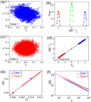
Figure 2: (Color online) Solving the inverse problem by double correlation matrix (DCM) method of algorithms (5) and (6). $N=100$. $500$ active links and $500$ repressive ones are randomly chosen, and $A_{ij}(0)=0$ for all other off-diagonal matrix elements. $L=5\times{10^{5}}$ samples are yielded for inferences. (a)(b) Case 1: Jacobian matrix $\hat{\mathbf{A}}$ is given as: active interactions $A(a)_{ij}=1$; repressive interactions $A(r)_{ij}=-1$; the diagonal terms are set to $A_{ii}=-3$; and noise correlation matrix is given as $\hat{\mathbf{Q}}_{ij}=\sigma_{i}\delta_{ij},\sigma_{i}=0.01$. (c)(d) Case 2: The same as (a)(b) with heterogeneous $\hat{\mathbf{A}}$ and $\hat{\mathbf{Q}}$, i.e., $A_{ij}(a)\in(1.0,2.0)$ and $A_{ij}(r)\in(-2.0,-1.0)$ with uniform distributions, $A_{ii}=-5$, and $\sigma_{i}\in(0.005,0.015)$ with uniform distribution. (a)(c) The trajectories in a $2D$ phase plane for the two sets of networks and parameters. (b) The distribution of off-diagonal elements of $\hat{\mathbf{A}}=\hat{\mathbf{B}}\hat{\mathbf{C}}^{-1}$ (blue triangles for $A_{ij}(a)$, red squares for $A_{ij}(r)$, and green circles for $A_{ij}(0)$) calculated by Eq. (5) from data of (a). The computational elements of matrix $\hat{\mathbf{B}}\hat{\mathbf{C}}^{-1}$ coincide very well with the actual $\hat{\mathbf{A}}$, and all active, repressive and null interactions can be accurately predicted. (d) Matrix elements computed by $\hat{\mathbf{B}}\hat{\mathbf{C}}^{-1}$ are plotted against true Jacobian matrix elements $A_{ij}$ for Case 2 (all colors have the same meaning as (b)). All dots locate closely near the diagonal line, indicating correct inferences of both interaction natures and coupling strengths. (e) Element values of $-2\hat{\mathbf{B}}_{s}$ plotted versus element values of actual $\hat{\mathbf{Q}}$ for both the noises of (a)(c). The agreements between $-2\hat{\mathbf{B}}_{s}$ and $\hat{\mathbf{Q}}$ convincingly show that the DCM method can depict not only Jacobian matrix $\hat{\mathbf{A}}$ but also noise correlation matrix $\hat{\mathbf{Q}}$ merely from the output variable data. The task addressed in Fig. 1(d) is fulfilled indeed. (f) Standard deviation ($SD$) of Eq. (8) plotted against the number of samples $L$. $SD$s decay as $\frac{1}{\sqrt{L}}$. From this law we can predict the necessary sample numbers for different inference precisions.

Computational results. Equation (2) can be generally derived for any phase space point where output data are available and $\hat{\mathbf{A}}$ is thus $\mathbf{x}$ dependent. Around a stable steady state of noise-free system, we can linearize Eq. (1) directly around the fixed point ${\mathbf{x}}_{0}$ and set ${\mathbf{x}}={\mathbf{x}}_{0}$ and $\mathbf{y}(t)=\mathbf{x}(t)-{\mathbf{x}}_{0}$ for computing (4)-(7). Now, our task is to reveal both Jacobian matrix $\hat{\mathbf{A}}$ in (2) and noise correlation $\hat{\mathbf{Q}}$ in (3) from measurable variable data $\mathbf{y}(t)$.

In Fig. 2 we consider two examples for numerical simulations. The network size in Figs. 2(a)(b) (Case 1) is $N=100$. Among $10^{4}$ links there are $500$ active links $A_{ij}(a)=1$ and $500$ repressive ones $A_{ij}(r)=-1$ arbitrarily chosen, $A_{ij}(0)=0$ for all else off-diagonal matrix elements, and the diagonal terms are set to $A_{ii}=-3$ for keeping the network evolution bounded. Moreover, we take $\hat{\mathbf{Q}}_{ij}=\sigma_{i}\delta_{ij},\sigma_{i}=0.01$. Running system (2) from $y_{i}(t=0)=0$ we produce $L=5\times 10^{5}$ sets of data. Assume we know nothing about network structure $\hat{\mathbf{A}}$ and noise statistics $\hat{\mathbf{Q}}$ but only the data sequences of $\mathbf{y}(t)$, among which a projective trajectory is plotted in a $2D$ ($y_{1}(t)$, $y_{2}(t)$) phase plane in Fig. 2(a), which seems fully disordered. All the elements of matrices $\hat{\mathbf{B}}$ and $\hat{\mathbf{C}}$ can be computed from the data $\mathbf{y}(t)$ with Eqs. (4)(7), and then matrix $\hat{\mathbf{A}}$ can be retrieved by Eq. (5). The results are presented in Fig. 2(b) where interactions depicted by $\hat{\mathbf{B}}\hat{\mathbf{C}}^{-1}$ agree well with the actual interactions $\hat{\mathbf{A}}$. In Figs. 2(c)(d) (Case 2), we do the same as Figs. 2(a)(b) with the noise statistics changed to $\hat{\mathbf{Q}}_{ij}=\sigma_{i}\delta_{ij}$ with $\sigma_{i}\in(0.005,0.015)$, and $A_{ij}$ set to $A_{ij}(a)\in(1.0,2.0)$, $A_{ij}(r)\in(-2.0,-1.0)$ (all randomly chosen with uniform distributions in their ranges) and the diagonal terms are set to $A_{ii}=-5$. Though the trajectory behaviors of Figs. 2(a) and 2(c) deviate from each other substantially due to different noise correlations $\hat{\mathbf{Q}}$ and Jacobian matrix $\hat{\mathbf{A}}$, and these different data sets can surely yield considerably different matrices $\hat{\mathbf{B}}$ and $\hat{\mathbf{C}}$, it is remarkable that in Figs. 2(b) and 2(d) the DCM method can correctly deduce both interaction matrices $\hat{\mathbf{A}}$ by applying the same algorithm $\hat{\mathbf{A}}=\hat{\mathbf{B}}\hat{\mathbf{C}}^{-1}$. On the contrary, most of inference methods use only correlations of $\hat{\mathbf{C}}$ (or other related quantities) and the results of these methods are thus seriously influenced by noise, and can never produce correct inferences with a universal formula for different noise correlations.

For confirming the conclusions of Eq. (6), we plot $-2\hat{\mathbf{B}}_{s}$ computed from the variable data against actual noise statistics $\hat{\mathbf{Q}}$ in Fig. 2(e) for the two data sets of Figs. 2(a) and 2(c). All these dots locate very closely around the diagonal line, convincingly justifying the prediction of Eq. (6). The results of Eqs. (5)(6) are exact in the limits of white noise and $L\rightarrow{\infty}$, $\Delta{t_{q}}\rightarrow 0$. In Fig. 2(f) we use the systems of Figs. 2(a) and 2(c) to numerically compute the standard deviation ($SD$) of inferred values of interactions defined as

$$SD(L)=\sqrt{\frac{\sum_{i=1}^{N}\sum_{j=1}^{N}{([BC^{-1}]_{ij}-A_{ij})^{2}}}{N^{2}}},$$ (8)

where summations of $i$ and $j$ run over all matrix elements and $L$ is the total number of computational samples. It is clear that $SD{\propto}{\frac{1}{\sqrt{L}}}$, agreeing with the conclusion of exact inference solutions for $L\rightarrow{\infty}$. The theoretical conclusion that algorithms (5) and (6) can reveal both interaction structure $\hat{\mathbf{A}}$ and noise statistics $\hat{\mathbf{Q}}$ are remarkably verified by numerical simulations based on which we can, for the first time, reconstruct the stochastic dynamic networks Eq. (2) from their variable outputs only. And this capacity of the DCM method is unique in all known inference methods.

In Fig. 2 we study the inverse problem of noise-driven randomly constructed networks around stable fixed points. The DCM method can be generally applicable to various dynamic networks described by coupled stochastic ODEs, i.e., to different noise-free states such as periodic oscillations (SM II) and even chaotic states (SM III); to different network topologies such as scale-free networks (SM III).

The currently prevailing inference methods are based on different information included in the output data to infer network structures. In SM IV, three commonly-used methods (Pearson correlation, Mutual information and Regression) are introduced for comparisons with the DCM method. For the noise-generated data, the results of the DCM method are considerably better than those of all the three commonly-used methods in both qualitative and quantitative predictions.

Conclusion. In conclusion, we proposed a double correlation matrix (DCM) method to infer noise-driven dynamic networks from their output data. For given output time sequences yielded by stochastic network dynamics, the DCM method can accurately depict network structures with a compact formula. The method can depict not only the qualitative features of network structures (e.g., active, repressive and null natures of interactions), but also the precise strengths of interactions; not only the interaction Jacobian matrix $\hat{\mathbf{A}}$, but also the noise correlations $\hat{\mathbf{Q}}$. These are far beyond the capacity of all known inference methods.

There are two major ingredients enable the advantages of the DCM method. First, this method can extract more information because it measures not only the available data but also the variation velocities of variables while in most of inference methods only the former data have been used. The joint application of these two types of data makes the DCM method capable to infer network interactions much more accurately than other existing methods (see SM IV). Moreover, the DCM method uses the fast varying property of white noise (which is valid in most of realistic systems) so that matrix $\hat{\mathbf{B}}$ in Eq. (5) can filter out noise effectively and then infer network structures without any knowledge of noise statistics (Fig. 1(d)). This has never been regarded possible so far.

Some conditions are required for the DCM method. The data should contain information of velocities of variables for computing matrix $\hat{\mathbf{B}}$. For doing so sufficiently fast data measurements are required. Since noise plays crucial role in yielding data, sufficiently large data sets are necessary for filtering out the noise contaminations. Many practically important systems can fulfill these conditions, among which brain networks and financial networks (e.g., stock market evolutions) are the most interesting candidates. In both cases, noises are often crucial in generating activity data and various quickly developed techniques guarantee high-frequency and non-invasive measurements and huge data collections. It is our further works to analyze these data sets to depict the possibly hidden network structures from dynamic variable data by applying the DCM method.

Acknowledgments. This work is supported by National Foundation of Natural Science of China Grants 11135001 and 11174034 (to G.H.), 11075016 (to Z.Z.), 11305112 (to Y.M.), and 91132702 and 31261160495 (to S.W.); the Open Research Fund of the State Key Laboratory of Cognitive Neuroscience and Learning (CNLYB1211); and Natural Science Foundation of Jiangsu Province BK20130282.

References

- Butte et al. (2000) A. J. Butte, P. Tamayo, D. Slonim, T. R. Golub, and I. S. Kohane, Proceedings of the National Academy of Sciences 97, 12182 (2000).
- Kim et al. (2001) S. K. Kim, J. Lund, M. Kiraly, K. Duke, M. Jiang, J. M. Stuart, A. Eizinger, B. N. Wylie, and G. S. Davidson, Science 293, 2087 (2001).
- Bar-Joseph et al. (2012) Z. Bar-Joseph, A. Gitter, and I. Simon, Nat Rev Genet 13, 552 (2012).
- Bar-Joseph et al. (2003) Z. Bar-Joseph, G. K. Gerber, T. I. Lee, N. J. Rinaldi, J. Y. Yoo, F. Robert, D. B. Gordon, E. Fraenkel, T. S. Jaakkola, R. A. Young, et al., Nat Biotech 21, 1337 (2003).
- De Smet and Marchal (2010) R. De Smet and K. Marchal, Nat Rev Micro 8, 717 (2010).
- Feist et al. (2009) A. M. Feist, M. J. Herrgard, I. Thiele, J. L. Reed, and B. O. Palsson, Nat Rev Micro 7, 129 (2009).
- Barzel and Barabasi (2013) B. Barzel and A.-L. Barabasi, Nat Biotech 31, 720 (2013).
- Feizi et al. (2013) S. Feizi, D. Marbach, M. Medard, and M. Kellis, Nat Biotech 31, 726 (2013).
- Stuart et al. (2003) J. M. Stuart, E. Segal, D. Koller, and S. K. Kim, Science 302, 249 (2003).
- Hu et al. (2007) Z. Hu, P. J. Killion, and V. R. Iyer, Nat Genet 39, 683 (2007).
- Yeung et al. (2002) M. K. S. Yeung, J. Tegnér, and J. J. Collins, Proceedings of the National Academy of Sciences 99, 6163 (2002).
- Lezon et al. (2006) T. R. Lezon, J. R. Banavar, M. Cieplak, A. Maritan, and N. V. Fedoroff, Proceedings of the National Academy of Sciences 103, 19033 (2006).
- Segal et al. (2003) E. Segal, M. Shapira, A. Regev, D. Pe’er, D. Botstein, D. Koller, and N. Friedman, Nat Genet 34, 166 (2003).
- Marbach et al. (2012) D. Marbach, J. C. Costello, R. Kuffner, N. M. Vega, R. J. Prill, D. M. Camacho, K. R. Allison, M. Kellis, J. J. Collins, and G. Stolovitzky, Nat Meth 9, 796 (2012).
- Marbach et al. (2010) D. Marbach, R. J. Prill, T. Schaffter, C. Mattiussi, D. Floreano, and G. Stolovitzky, Proceedings of the National Academy of Sciences 107, 6286 (2010).
- Bullmore and Sporns (2009) E. Bullmore and O. Sporns, Nat Rev Neurosci 10, 186 (2009).
- Sugihara et al. (2012) G. Sugihara, R. May, H. Ye, C.-h. Hsieh, E. Deyle, M. Fogarty, and S. Munch, Science 338, 496 (2012).
- Arkin et al. (1997) A. Arkin, P. Shen, and J. Ross, Science 277, 1275 (1997).
- Arkin and Ross (1995) A. Arkin and J. Ross, J. Phys. Chem. 99, 970 (1995).
- Barabasi and Oltvai (2004) A.-L. Barabasi and Z. N. Oltvai, Nat Rev Genet 5, 101 (2004).
- Barabasi and Albert (1999) A.-L. Barabasi and R. Albert, Science 286, 509 (1999).
- Watts and Strogatz (1998) D. J. Watts and S. H. Strogatz, Nature 393, 440 (1998).
- Glass and Mackey (1988) L. Glass and M. C. Mackey, From Clocks to Chaos: The Rhythms of Life (Princeton University Press, Princeton, NJ, 1988).
- Goldbeter (1996) A. Goldbeter, Biochemical Oscillations and Cellular Rhythms (Cambridge University Press, Cambridge, UK, 1996).
- Tsai et al. (2008) T. Y.-C. Tsai, Y. S. Choi, W. Ma, J. R. Pomerening, C. Tang, and J. E. Ferrell, Science 321, 126 (2008).
- Alon (2007) U. Alon, Introduction to Systems Biology: Design Principles of Biological Networks (CRC press, 2007).
- Basso et al. (2005) K. Basso, A. A. Margolin, G. Stolovitzky, U. Klein, R. Dalla-Favera, and A. Califano, Nat Genet 37, 382 (2005).
- Bansal et al. (2007) M. Bansal, V. Belcastro, A. Ambesi-Impiombato, and D. di Bernardo, Mol Syst Biol 3, (2007).
- Villaverde et al. (2013) A. F. Villaverde, J. Ross, and J. R. Banga, Cells 2, 306 (2013).
- Jansen et al. (2003) R. Jansen, H. Yu, D. Greenbaum, Y. Kluger, N. J. Krogan, S. Chung, A. Emili, M. Snyder, J. F. Greenblatt, and M. Gerstein, Science 302, 449 (2003).
- Friedman (2004) N. Friedman, Science 303, 799 (2004).
- Haury et al. (2012) A.-C. Haury, F. Mordelet, P. Vera-Licona, and J.-P. Vert, BMC Systems Biology 6, 145 (2012).
- Gardner et al. (2003) T. S. Gardner, D. di Bernardo, D. Lorenz, and J. J. Collins, Science 301, 102 (2003).
- Covert et al. (2004) M. W. Covert, E. M. Knight, J. L. Reed, M. J. Herrgard, and B. O. Palsson, Nature 429, 92 (2004).
- Eisen et al. (1998) M. B. Eisen, P. T. Spellman, P. O. Brown, and D. Botstein, Proceedings of the National Academy of Sciences 95, 14863 (1998).
- Faith et al. (2007) J. J. Faith, B. Hayete, J. T. Thaden, I. Mogno, J. Wierzbowski, G. Cottarel, S. Kasif, J. J. Collins, and T. S. Gardner, PLoS Biol 5, e8 (2007).
- Ren et al. (2010) J. Ren, W.-X. Wang, B. Li, and Y.-C. Lai, Phys. Rev. Lett. 104, 058701 (2010).
- Levnaji and Pikovsky (2014) Z. Levnaji and A. Pikovsky, Sci. Rep. 4, (2014).
- Ching et al. (2013) E. S. C. Ching, P.-Y. Lai, and C. Y. Leung, Phys. Rev. E 88, 042817 (2013).
- Risken (1984) H. Risken, The Fokker-Planck Equation (Springer-Verlag Berlin Heidelberg New York, 1984).
- Wang et al. (2009) W.-X. Wang, Q. Chen, L. Huang, Y.-C. Lai, and M. A. F. Harrison, Phys. Rev. E 80, 016116 (2009).