Imaging with Kantorovich-Rubinstein discrepancy

Abstract

We propose the use of the Kantorovich-Rubinstein norm from optimal transport in imaging problems. In particular, we discuss a variational regularisation model endowed with a Kantorovich-Rubinstein discrepancy term and total variation regularization in the context of image denoising and cartoon-texture decomposition. We point out connections of this approach to several other recently proposed methods such as total generalized variation and norms capturing oscillating patterns. We also show that the respective optimization problem can be turned into a convex-concave saddle point problem with simple constraints and hence, can be solved by standard tools. Numerical examples exhibit interesting features and favourable performance for denoising and cartoon-texture decomposition.

1 Introduction

Distance functions related to ideas from optimal transport have appeared in various places in imaging problems in the last ten years. The main applications in this context are image and shape classification [36, 37, 38, 40, 39, 45, 51, 58], segmentation [16, 44, 48, 55, 56], registration and warping [27, 63, 46], image smoothing [11], contrast and colour modification [50, 22], texture synthesis and texture mixing [52], and surface mapping [32, 33, 6, 10]. Being a distance function applicable to very general densities (continuous and discrete (Dirac deltas) densities) the Wasserstein distance had an increasing impact on robust distance measures in imaging [54, 12, 26, 31, 61, 52, 48, 11]. In most cases, the 2-Wasserstein distance [2] is used.

In this work we propose the use of the so-called Kantorovich-Rubinstein norm ($\operatorname{KR}$-norm) in imaging. We investigate the $\operatorname{KR}$-$\operatorname{TV}$ denoising problem, that is, for a given noisy image $u^{0}$ on a set $\Omega$ and two constants $\lambda_{1},\lambda_{2}\geq 0$ we consider

$$\min_{u}\|u-u^{0}\|_{\operatorname{KR},(\lambda_{1},\lambda_{2})}+\operatorname{TV}(u)$$

where the $\operatorname{KR}$-norm is defined for a Radon measure $\mu$ (and hence, also for $L^{1}$-functions) on a set $\Omega\subset\mathbb{R}^{n}$ by

$$\|\mu\|_{\operatorname{KR},(\lambda_{1},\lambda_{2})}=\sup\{\int_{\Omega}f\,\mathrm{d}\mu\ :\ |f|\leq\lambda_{1},\ \operatorname{Lip}(f)\leq\lambda_{2}\}.$$

The Kantorovich-Rubinstein norm [5, §8.3] is closely related to the 1-Wasserstein distance and hence, to optimal transport problems. It will turn out that this norm has interesting relations to other well known concepts in imaging: The KR-norm is a generalization of the $L^{1}$ norm, and hence, a $\operatorname{KR}$-$\operatorname{TV}$ denoising model inherits and generalizes some of the favorable properties of the $L^{1}$-TV denoising [15]. The generalization of $L^{1}$-norm discrepancies to $\operatorname{KR}$-norm discrepancies shares some similarities with the generalization from the TV penalty to the total generalized variation (TGV) penalty [7]. Finally, the KR-norm discrepancy shares properties with Meyer’s $G$-norm model [41, 59] for oscillating patterns and for cartoon-texture decomposition. Also from the computational point of view, the $\operatorname{KR}$-norm has favorable properties. It turns out that the $\operatorname{KR}$-$\operatorname{TV}$ denoising problem has a formulation as a saddle-point problem that can be solved by means of several primal-dual methods. The computational cost per iteration as well as the needed storage requirements are almost as low as for similar algorithms for $L^{1}$-$\operatorname{TV}$ denoising.

The paper is organized as follows: After fixing the notation we introduce and recall transport metrics in Section 2. In Section 3 we derive two reformulations of the $\operatorname{KR}$-norm that will be used to analyze and interpret the $\operatorname{KR}$-$\operatorname{TV}$ denoising problem, which is the content of Section 4. In Section 5 we illustrate how the $\operatorname{KR}$-$\operatorname{TV}$ denoising problem can be solved numerically by primal dual methods. Finally, in Section 6 we present examples for $\operatorname{KR}$-$\operatorname{TV}$ denoising and cartoon-texture decomposition and then finish the paper with a conclusion.

1.1 Notation

We work in a domain $\Omega\subset\mathbb{R}^{n}$ and use $|x|$ as the euclidean absolute value for $x\in\Omega$. We denote by $\mathfrak{M}(\Omega,\mathbb{R}^{n})$ the space of $\mathbb{R}^{n}$-valued Radon measures, i.e. the dual space of $(C_{0}(\Omega,\mathbb{R}^{n}),\||\cdot|\|_{\infty})$ of continuous functions that vanish “at infinity”. If we want to emphasize that a function or a measure is vector valued we write $\vec{\nu}$ but sometime we omit the emphasis. The dual pairing between $\mathfrak{M}(\Omega,\mathbb{R}^{n})$ and $C_{0}(\Omega,\mathbb{R}^{n})$ (and any two other spaces in duality) will be denoted by $\langle\vec{f},\vec{\mu}\rangle$. Consequently, the norm on $\mathfrak{M}(\Omega,\mathbb{R}^{n})$ is $\|\vec{\mu}\|_{\mathfrak{M}}=\sup_{|\vec{f}|\leq 1}\int\vec{f}\cdot\,\mathrm{d}\vec{\mu}$ and is called the Radon norm. We identify $u\in L^{1}(\Omega,\mathbb{R}^{n})$ with the corresponding measure $u\in\mathfrak{M}(\Omega,\mathbb{R}^{n})$, i.e. we treat $L^{1}(\Omega,\mathbb{R}^{n})$ embedded into $\mathfrak{M}(\Omega,\mathbb{R}^{n})$. The $n$-dimensional Lebesgue measure is denoted by $\mathfrak{L}^{n}$ while the $d$-dimensional Hausdorff measure is $\mathfrak{H}^{d}$.

For a measure $\mu$ on $\Omega$, another set $\Omega^{\prime}$ and $F:\Omega\to\Omega^{\prime}$ the push-forward of $\mu$ by $F$ is $\mu\#F(A)=\mu(F^{-1}(A))$. On $\Omega\times\Omega$ we denote by $\operatorname{proj}_{1/2}$ the projections onto the first and second component, respectively. Having a measure $\gamma$ on $\Omega\times\Omega$ we denote (with slight abuse of notation) by $\operatorname{proj}_{1/2}\gamma$ the push forward of $\gamma$ by $\operatorname{proj}_{1/2}$, i.e. the marginals of $\gamma$. The restriction of some measure $\mu$ onto some set $A$ is denoted by $\mu\llcorner A$. By $C_{b}(\Omega,\mathbb{R}^{n})$ we denote the space of bounded and continuous functions on $\Omega$. For $f:\Omega\to\mathbb{R}$ we denote by $\operatorname{Lip}(f)=\sup_{x\neq y}|f(x)-f(y)|/|x-y|$ the Lipschitz constant of $f$.

For two points $a,b\in\mathbb{R}^{n}$ we define the line interval $[a,b]=\{ta+(1-t)b\mid t\in[0,1]\}$ and the vector measure $\llbracket a,b\rrbracket$ to be

$$\llbracket a,b\rrbracket=\frac{b-a}{|b-a|}\mathfrak{H}^{1}\llcorner[a,b].$$

By $\operatorname{diam}(\Omega)=\sup\{|x-y|\ :\ x,y\in\Omega\}$ we denote the diameter on $\Omega$. For a set $C$ we denote by $I_{C}$ the indicator function, i.e. $I_{C}(u)=0$ for $u\in C$ and $=\infty$ otherwise.

2 Transport metrics

A variety of different metrics exist on measure spaces. As the study of metrics on measure spaces has its origins in probability theory, most metrics are defined on the space of probability measures, i.e., non-negative measures with total mass equal to one. A popular class of such metrics is given by the Wasserstein metrics: For $p\geq 1$ and two probability measures $\mu$ and $\nu$ define

$$W_{p}(\mu,\nu)=\Big{(}\inf\{\int_{\Omega\times\Omega}|x-y|^{p}\,\mathrm{d}\gamma(x,y)\ :\ \operatorname{proj}_{1}\gamma=\mu,\ \operatorname{proj}_{2}\gamma=\nu\}\Big{)}^{1/p}.$$ (1)

Note that this metric also makes sense if $\mu$ and $\nu$ are not probability measures but still non-negative and have equal mass, i.e., $\int_{\Omega}\,\mathrm{d}\mu=\int_{\Omega}\,\mathrm{d}\nu$. However, if the mass is not equal, no $\gamma$ with $\mu$ and $\nu$ as marginals would exist.

The celebrated Kantorovich duality [28, 60] states that, in the case of non-negative measures with equal mass, the Wasserstein metric can be equivalently expressed as

$$W_{p}(\mu,\nu)=\Big{(}\sup\{\int_{\Omega}\phi\,\mathrm{d}\mu+\int_{\Omega}\psi\,\mathrm{d}\nu\ :\ \phi,\psi\in C_{b}(\Omega),\ \phi(x)+\psi(y)\leq|x-y|^{p}\}\Big{)}^{1/p}.$$

A particular special case is $p=1$, and here, the Kantorovich-Rubinstein duality [29, 60] states that

$$W_{1}(\mu,\nu)=\sup\{\int_{\Omega}f\,\mathrm{d}(\mu-\nu)\ :\ \operatorname{Lip}(f)\leq 1\}.$$

A particularly interesting fact is that this metric only depends on the difference $\mu-\nu$. In fact, by setting

$$\|\mu\|_{\operatorname{Lip}^{*}}=\sup\{\int_{\Omega}f\,\mathrm{d}\mu\ :\ \operatorname{Lip}(f)\leq 1\}$$

one obtains the so-called dual Lipschitz norm on the space of measures with zero mean and finite first moments (cf. [5, §8.10(viii)] where it is called modified Kantorovich-Rubinstein norm). Note that the supremum is unbounded if one has a nonzero mean. To prevent the norm from blowing up in this case, and hence, to obtain a norm on the space of all signed measures with finite first moments, one can add the constraint that the test functions $f$ shall be bounded. This leads to the expression

$$\sup\{\int_{\Omega}f\,\mathrm{d}\mu\ :\ |f|\leq 1,\ \operatorname{Lip}(f)\leq 1\}.$$

(which is called Kantorovich-Rubinstein norm in [5, §8.3]). Since we would like the bound on the values of $f$ and the bound on its Lipschitz constant to vary independently in the following, we introduce for $\lambda=(\lambda_{1},\lambda_{2})$ the norm

$$\|\mu\|_{\operatorname{KR},\lambda}=\sup\{\int_{\Omega}f\,\mathrm{d}\mu\ :\ |f|\leq\lambda_{1},\ \operatorname{Lip}(f)\leq\lambda_{2}\}$$ (2)

Note that in the extreme cases $\lambda_{1}=\infty$ and $\lambda_{2}=\infty$ we recover the dual Lipschitz and the Radon norm

$$\begin{split}\|\mu\|_{\operatorname{KR},(\infty,1)}&=\|\mu\|_{\operatorname{Lip}^{*}}\\ \|\mu\|_{\operatorname{KR},(1,\infty)}&=\|\mu\|_{\mathfrak{M}}.\end{split}$$ (3)

Note that the norm $\|\mu\|_{\operatorname{KR},(\lambda_{1},\lambda_{2})}$ with $\lambda_{1},\lambda_{2}>0$ is equivalent to the bounded Lipschitz norm [60, §6] where one takes the supremum over all functions $f$ such that $|f|+\operatorname{Lip}(f)\leq 1$. In general we have the following simple estimates:

Lemma 2.1 (Estimates by the Radon norm).

For any $\lambda=(\lambda_{1},\lambda_{2})\geq 0$ it holds that

$$\|\mu\|_{\operatorname{KR},\lambda}\leq\lambda_{1}\|\mu\|_{\mathfrak{M}}.$$

If $\mu$ is non-negative it holds that

$$\|\mu\|_{\operatorname{KR},\lambda}=\lambda_{1}\|\mu\|_{\mathfrak{M}}.$$

If $\Omega$ has finite diameter $\operatorname{diam}(\Omega)$, then it holds for any $\mu$ with $\int_{\Omega}\,\mathrm{d}\mu=0$ that

$$\|\mu\|_{\operatorname{KR},\lambda}\leq\lambda_{2}\tfrac{\operatorname{diam}(\Omega)}{2}\|\mu\|_{\mathfrak{M}}.$$

Proof.

The first inequality follows directly from the definition of $\|\mu\|_{\operatorname{KR},\lambda}$ by dropping the constraint $|\nabla f|\leq\lambda_{2}$ and the second claim by observing that the supremum is attained at $f\equiv\lambda_{1}$.

For the last claim we estimate from above by dropping the constraint $\|f\|_{\infty}\leq\lambda_{1}$. However, since $\Omega$ has bounded diameter and $\mu$ has mean value zero, the constraint $\||\nabla f|\|_{\infty}\leq\lambda_{2}$ implies that one also has a bound $\|f\|_{\infty}\leq\lambda_{2}\operatorname{diam}(\Omega)/2$ (indeed, $\lambda_{2}\operatorname{diam}(\Omega)$ is a bound on the value $\max f-\min f$, however, since $\int_{\Omega}\,\mathrm{d}\mu=0$, we may add a constant to $f$ without altering the outer supremum). We obtain

$$\|\mu\|_{\operatorname{KR},\lambda_{1},\lambda_{2}}\leq\sup\limits_{\|f\|_{\infty}\leq\lambda_{2}\operatorname{diam}(\Omega)/2}\int f\,\,\mathrm{d}\mu\leq\lambda_{2}\operatorname{diam}(\Omega)\|\mu\|_{\mathfrak{M}}/2.$$

∎

Remark 2.2.

Note that the $\operatorname{KR}$-norm may not be bounded from below by the Radon norm in general: For $\mu=\delta_{x_{0}}+\delta_{x_{1}}$ it holds that $\|\mu\|_{\mathfrak{M}}=2$ while $\|\mu\|_{\operatorname{KR},\lambda}\to 0$ for $|x_{0}-x_{1}|\to 0$.

3 Primal formulations of the $\operatorname{KR}$-norm

We present two reformulations of the $\operatorname{KR}$-norm. The first, only shown formally, is similar to the Kantorovich-Rubinstein duality and shows the relation to optimal transport.

The idea is to replace the constraint $\operatorname{Lip}(f)\leq\lambda_{2}$ by a pointwise constraint of the form $|f(x)-f(y)|\leq\lambda_{2}|x-y|$, i.e., we have

$$\|\mu\|_{\operatorname{KR},\lambda}=\sup\{\int f\,\mathrm{d}\mu\ :\ |f(x)|\leq\lambda_{1},\ |f(x)-f(y)|\leq\lambda_{2}|x-y|\}.$$

We express the pointwise constraints by $f(x)-\lambda_{1}\leq 0$, $-f(x)-\lambda_{1}\leq 0$, $f(x)-f(y)-\lambda_{2}|x-y|\leq 0$ and $f(y)-f(x)-\lambda_{2}|x-y|\leq 0$, introduce Lagrange multipliers and clean up the resulting expression and finally arrive at

$$\|\mu\|_{\operatorname{KR},\lambda}=\inf_{\gamma\geq 0}\Bigg{[}\lambda_{1}\int_{\Omega}\,\mathrm{d}|\mu-\operatorname{proj}_{1}\gamma+\operatorname{proj}_{2}\gamma|+\lambda_{2}\int_{\Omega\times\Omega}|x-y|\,\mathrm{d}\gamma\Bigg{]}.$$ (4)

This expression may be compared to the following variant from [53]

$$\|\mu\|_{\operatorname{KR}^{\prime}}=\inf_{\gamma\geq 0}\{\int_{\Omega\times\Omega}|x-y|\,\mathrm{d}\gamma\ :\ \operatorname{proj}_{1}\gamma-\operatorname{proj}_{2}\gamma=\mu\},$$

which is a “strict constraint” version of (4). Because we have a metric cost function $(x,y)\mapsto|x-y|$, this is the same as requiring $\operatorname{proj}_{1}\gamma=\mu^{+},\operatorname{proj}_{2}\gamma=\mu^{-}$ and we recover the Wasserstein metric with $p=1$ from (1).

We get another reformulation by dualizing the problem slightly differently. The idea is to reformulate the constraint $\operatorname{Lip}(f)\leq\lambda_{2}$ with the help of the distributional derivative of $f$ as $\||\nabla f|\|_{\infty}\leq\lambda_{2}$. This is allowed since for bounded, convex and open domains $\Omega$, it is indeed the case that $\||\nabla f|\|_{\infty}=\operatorname{Lip}(f)$ (cf. [1, Prop. 2.13]). Through this reformulation, the KR-norm can be seen to be equivalent to the flat norm in the theory of currents [43, 21].

Lemma 3.1.

Let $\Omega\subset\mathbb{R}^{n}$ be open, convex, and bounded, and let $\lambda=(\lambda_{1},\lambda_{2})\geq 0$. Then it holds that

$$\|\mu\|_{\operatorname{KR},\lambda}=\min_{\vec{\nu}\in\mathfrak{M}(\overline{\Omega},\mathbb{R}^{n})}\lambda_{1}\|\mu-\operatorname{div}\vec{\nu}\|_{\mathfrak{M}}+\lambda_{2}\||\vec{\nu}|\|_{\mathfrak{M}}$$ (5)

where $\operatorname{div}\vec{\nu}$ is understood to be taken in $\overline{\Omega}$ or, equivalently, in any open set $U$ containing $\overline{\Omega}$.

Proof.

We have

$$\|\mu\|_{\operatorname{KR},\lambda}=\sup_{f}\int_{\Omega}f\,\mathrm{d}\mu-I_{\{\|\cdot\|_{\infty}\leq\lambda_{1}\}}(f)-I_{\{\||\cdot|\|_{\infty}\leq\lambda_{2}\}}(\nabla f).$$

Now let $U$ be an open set containing $\overline{\Omega}$, define the Banach spaces $X=C_{c}^{1}(U)$ and $Y=C_{0}(U,\mathbb{R}^{n})$, and the subsets

$$A =\{f\in X\ :\ \sup_{x\in\overline{\Omega}}|f(x)|\leq\lambda_{1}\}$$

$$B =\{\vec{g}\in Y\ :\ \sup_{x\in\overline{\Omega}}|\vec{g}(x)|\leq\lambda_{2}\}.$$

Further define functionals $F:X\to\mathbb{R}\cup\{\infty\}$ and $G:Y\to\mathbb{R}\cup\{\infty\}$ by

$$F(f)=-\int_{\Omega}f\,\mathrm{d}\nu+I_{A}(f),\qquad G(\vec{g})=I_{B}(\vec{g})$$

as well as the linear operator $K=\nabla:X\to Y$. With this notation we have

$$\|\mu\|_{\operatorname{KR},\lambda}=\sup_{f\in X}F(f)+G(Kf).$$

To use the Fenchel-Rockafellar duality [20] we use the constraint qualification from [3], i.e., that it holds that

$$\bigcup_{\alpha>0}\alpha[\operatorname{dom}(G)-K\operatorname{dom}(F)]\supset\bigcup_{\alpha>0}\alpha A=Y.$$

Hence, we have

$$\sup_{f\in X}-F(f)-G(Kf)=\inf_{\nu\in Y^{*}}F^{*}(-K^{*}\nu)+G^{*}(\nu).$$

We have $X^{*}=\mathfrak{M}(U)$ and $Y^{*}=\mathfrak{M}(U,\mathbb{R}^{n})$ and the conjugate functions of $F$ and $G$ are expressed with the help of the sets

$$C =\{\eta\in\mathfrak{M}(U)\ :\ |\eta|(U\setminus\overline{\Omega})=0\}$$

$$D =\{\vec{\nu}\in\mathfrak{M}(U,\mathbb{R}^{n})\ :\ |\vec{\nu}|(U\setminus\overline{\Omega})=0\}$$

as

$$F^{*}(\eta)=\lambda_{1}\|\mu+\eta\|_{\mathfrak{M}(\overline{\Omega})}+I_{C}(\eta),\qquad G^{*}(\vec{\nu})=\lambda_{2}\||\vec{\nu}|\|_{\mathfrak{M}(\overline{\Omega})}+I_{D}(\vec{\nu})$$

Since by the Kirszbraun theorem every $f$ that is Lipschitz continuous on $\Omega$ can be extended to $U$ (with preservation of the Lipschitz constant) it follows with $K^{*}=-\operatorname{div}:Y^{*}\to X^{*}$ that

$$\|\mu\|_{\operatorname{KR},\lambda} =\inf_{\vec{\nu}\in Y^{*}}F^{*}(-K^{*}\vec{\nu})+G^{*}(\vec{\nu})$$

$$=\inf_{\nu\in\mathfrak{M}(U,\mathbb{R}^{n})}\lambda_{1}\|\mu-\operatorname{div}\vec{\nu}\|_{\mathfrak{M}(U)}+\lambda_{2}\||\vec{\nu}|\|_{\mathfrak{M}(U)}+I_{C}(\operatorname{div}\vec{\nu})+I_{D}(\vec{\nu}).$$

Since bounded sets in $\mathfrak{M}(U,\mathbb{R}^{n})$ are relatively weakly* compact, we can replace the infimum by a minimum and since $\operatorname{supp}\vec{\nu}\subset\overline{\Omega}$ implies that $\operatorname{supp}\operatorname{div}\vec{\nu}\subset\overline{\Omega}$ we can replace $\mathfrak{M}(U,\mathbb{R}^{n})$ by $\mathfrak{M}(\overline{\Omega},\mathbb{R}^{n})$ and drop the constraints $C$ and $D$ and arrive at

$$\|\mu\|_{\operatorname{KR},\lambda}=\min_{\nu\in\mathfrak{M}(\overline{\Omega},\mathbb{R}^{n})}\lambda_{1}\|\mu-\operatorname{div}\vec{\nu}\|_{\mathfrak{M}(\overline{\Omega})}+\lambda_{2}\||\vec{\nu}|\|_{\mathfrak{M}(\overline{\Omega})}$$

as desired. ∎

In Theorem 3.4 below we will prove that actually we can take $\vec{\nu}$ as an $L^{1}$ vector field with $L^{1}$ divergence in (5). Namely $\vec{\nu}\in W^{1,1}(\Omega;\operatorname{div})$, where for $\Omega\subset\mathbb{R}^{n}$ an open domain, we define

$$W^{1,1}(\Omega;\operatorname{div}):=\{\vec{\nu}\in L^{1}(\Omega;\mathbb{R}^{n})\mid\operatorname{div}\vec{\nu}\in L^{1}(\Omega)\}.$$

As such, our result is closely related to the work in [17], where this $L^{1}$ property is proved for the transport density $|\vec{\nu}|$. Our proof is however different and shorter, based on the following simpler geometric estimate.

Lemma 3.2.

Let $\Omega\subset\mathbb{R}^{n}$ be convex, open and bounded, and $\mu=\sum_{i=1}^{N}\alpha_{i}\delta_{x_{i}}$. Then any optimal solution $\nu$ to (5) has the form $\nu=\sum_{j=1}^{M}\beta_{j}\llbracket a_{j},b_{j}\rrbracket$, where $a_{j},b_{j}=x_{i}$ for some $i$. Moreover, the transport rays $[a_{j},b_{j}]$ are approximately parallel in the following sense: there exist constants $c=c(n)$ and $\kappa=\kappa(n)$ such that if $[a_{j},b_{j}]\cap B(x,\rho)\neq\emptyset$ and $[a_{k},b_{k}]\cap B(x,\rho)\neq\emptyset$ with $a_{j},b_{j},a_{k},b_{k}\not\in B(x,c\rho)$, then $[a_{j},b_{j}]$ and $[a_{k},b_{k}]$ satisfy $a_{j},b_{j},a_{k},b_{k}\in B(x,2\kappa\rho)+\mathbb{R}z$ for some unit vector $z$.

Proof.

The claim that $\nu$ has the form $\nu=\sum_{j=1}^{M}\beta_{j}\llbracket a_{j},b_{j}\rrbracket$ is trivial, as the problem in (5) with discrete $\mu$ is a simple combinatorial problem.

Suppose $[a_{j},b_{j}]\cap B(x,\rho)\neq\emptyset$ and $[a_{k},b_{k}]\cap B(x,\rho)\neq\emptyset$, and that $a_{j},b_{j},a_{k},b_{k}\not\in B(x,c\rho)$, for $c$ yet to be determined. If $n=2$, let $\bar{a}_{j}:=a_{j}$, $\bar{b}_{j}:=b_{j}$, $\bar{a}_{k}:=a_{k}$, and $\bar{b}_{k}:=b_{k}$. Also set $d:=0$, and $v:=0$. Otherwise, if $n>2$, let $v\in\mathbb{R}^{n}$ be the vector giving the minimum distance between the lines

$$L_{j}:=a_{j}+\mathbb{R}(b_{j}-a_{j}),\quad\text{and}\quad L_{k}:=a_{k}+\mathbb{R}(b_{k}-a_{k}).$$

We may then find a plane $P\subset\mathbb{R}^{n}$ orthogonal to $v$ such that $L_{j}\subset P$ and $L_{k}\subset v+P$. After rotation and translation, if necessary, we may without loss of generality assume that $v=(0,d)\in\mathbb{R}^{n}$ for some $d\in\mathbb{R}^{n-2}$, and

$$a_{j}=(\bar{a}_{j},0),\ b_{j}=(\bar{b}_{j},0),\quad\text{and}\quad a_{k}=(\bar{a}_{k},d),\ b_{k}=(\bar{b}_{k},d).$$

We also denote $x=(\bar{x},x_{0})$. Since $L_{j}$ and $L_{k}$ lie on the planes $P$ and $v+P$ at a constant distance $\|d\|\leq 2\rho$ apart, we find that $\bar{a}_{j},\bar{b}_{j},\bar{a}_{k},\bar{b}_{k}\not\in B(\bar{x},\gamma_{n}c\rho)$, for some dimensional constant $\gamma_{n}\in(0,1)$. In fact, we may assume by shifting all of the points closer towards $x$ that

$$\bar{a}_{j},\bar{b}_{j},\bar{a}_{k},\bar{b}_{k}\in\partial B(\bar{x},\gamma_{n}c\rho),$$

This is possible with $c>1$ as the segments $[\bar{a}_{j},\bar{b}_{j}]$ and $[\bar{a}_{k},\bar{b}_{k}]$ pass through $B(\bar{x},\rho)$, and so we may split each segment into three parts – two outside $B(\bar{x},\gamma_{n}c\rho)$, and one inside.

Let $\kappa>2$. Observe now that in case $n=2$ and generally for $n>2$, when looking from the direction $v$, we have one of the two-dimensional situation depicted in Figure 11(a) or 1(b). The segments $[\bar{a}_{j},\bar{b}_{j}]$ and $[\bar{a}_{k},\bar{b}_{k}]$, starting and ending on $\partial B(\bar{x},\gamma_{n}c\rho)$, both pass through approximately ($c\gg 1$) in the middle of this sphere, through $\partial B(x,\rho)$. They are either within a cylinder of width $2\kappa\rho$, as in Figure 11(b), or are not, as in Figure 11(a).

If $\|a_{j}-a_{k}\|<\kappa\rho$ and $c$ is large enough that $B(x,\rho)$ reduces to almost to a point in comparison to $B(x,\gamma_{n}c\rho)$, then $\|\bar{b}_{j}-\bar{b}_{k}\|<2\kappa\rho$. This is because both segments $[\bar{a}_{j},\bar{b}_{j}]$ and $[\bar{a}_{k},\bar{b}_{k}]$ also pass through the ball $B(x,\rho)$ and so cannot diverge much on the opposite side of the ball. Trivially a unit vector $z$ exists, such that both segments lie in the cylinder $B(x,2\kappa\rho)+\mathbb{R}z$. Otherwise, for large enough $c$, both $|\bar{a}_{j}-\bar{a}_{k}|\geq\kappa\rho$ as well as $|\bar{b}_{j}-\bar{b}_{k}|>\kappa\rho$. Since $d\leq 2\rho<\kappa\rho$, i.e., some midpoints of the segments are closer than the end points, we observe that the two segments have to cross. That is $[\bar{a}_{j},\bar{b}_{j}]\cap[\bar{a}_{k},\bar{b}_{k}]=\bar{q}$ for some $\bar{q}$. If $c$ and $\kappa$ are large enough that $B(x,\rho)$ reduces to a point in comparison to everything else, we can make $\bar{q}\in B(\bar{x},\rho)$. By simple geometrical reasoning, on the triangle $\bar{a}_{j}-\bar{q}-\bar{b}_{k}$, compare Figure 11(c), it now follows that

$$|\bar{a}_{j}-\bar{b}_{k}|\leq\sqrt{|\bar{a}_{j}-\bar{q}|^{2}-(\kappa-2)^{2}\rho^{2}}+\sqrt{|\bar{b}_{k}-\bar{q}|^{2}-(\kappa-2)^{2}\rho^{2}}.$$

Likewise

$$|\bar{a}_{k}-\bar{b}_{j}|\leq\sqrt{|\bar{a}_{k}-\bar{q}|^{2}-(\kappa-2)^{2}\rho^{2}}+\sqrt{|\bar{b}_{j}-\bar{q}|^{2}-(\kappa-2)^{2}\rho^{2}}.$$

If $n=2$, or more generally $d=0$, it trivially follows that

$$\begin{split}|a_{j}-b_{k}|+|a_{k}-b_{j}|&<|a_{j}-q|+|b_{k}-q|+|a_{k}-q|+|b_{j}-q|\\ &=|a_{j}-b_{j}|+|a_{k}-b_{k}|.\end{split}$$

Otherwise, minding that $|d|\leq 2\rho$ and $\kappa>2$, we calculate

$$\begin{split}|a_{j}-b_{k}|+|a_{j}-b_{k}|&=\sqrt{|\bar{a}_{j}-\bar{b}_{k}|^{2}+|d|^{2}}+\sqrt{|\bar{a}_{k}-\bar{b}_{j}|^{2}+|d|^{2}}\\ &\leq\sqrt{(|\bar{a}_{j}-\bar{q}|+|\bar{b}_{k}-\bar{q}|)^{2}-2(\kappa-2)^{2}\rho^{2}+d^{2}}\\ &\phantom{\leq}+\sqrt{(|\bar{a}_{k}-\bar{q}|+|\bar{b}_{j}-\bar{q}|)^{2}-2(\kappa-2)^{2}\rho^{2}+d^{2}}\\ &<|a_{j}-q|+|b_{k}-q|+|a_{k}-q|+|b_{j}-q|\\ &=|a_{j}-b_{j}|+|a_{k}-b_{k}|.\end{split}$$

This provides a contradicion to the optimality of the transport rays $[a_{j},b_{j}]$ and $[a_{k},b_{k}]$, and shows the claim. ∎

Remark 3.3.

If $n=2$, we can take $\kappa=2$, and the argument is simplified considerably.

(a) Approximately parallel case

(b) Intersecting case

(c) Improvement of transport ray

Figure 1: Illustration of the two-dimensional projection in the proof of Lemma 3.2.

Theorem 3.4.

Suppose $\Omega\subset\mathbb{R}^{n}$ is convex, open, and bounded, and $\mu\in L^{1}(\Omega)$. Then

$$\|\mu\|_{\operatorname{KR},\lambda_{1},\lambda_{2}}=\min_{\nu\in W^{1,1}(\Omega;\operatorname{div})}\lambda_{1}\|\mu-\operatorname{div}\nu\|_{L^{1}(\Omega;\mathbb{R}^{n})}+\lambda_{2}\|\nu\|_{L^{1}(\Omega)}.$$ (6)

Moreover the minimum is reached by $\nu$ satisfying $\int_{\Omega}\operatorname{div}\nu\,\mathrm{d}\mathfrak{L}^{n}=0$.

Proof.

We assume first that $\mu\in L^{\infty}(\Omega)$. By Lemma 3.1, we have (5). To replace $\overline{\Omega}$ by $\Omega$, we just have to show that that $|\nu|(\partial\Omega)=0$ for any $\nu$ reaching the minimum in (5). This follows if $\nu\ll\mathfrak{L}^{n}$. Hence it suffices to show that actually $\nu$ and $\operatorname{div}\nu$ are also absolutely continuous with respect to $\mathfrak{L}^{n}$. This is where we need the convexity of $\Omega$ and the absolute continuity of $\mu$.

Clearly by (5) we have

$$\|\mu\|_{\operatorname{KR},\lambda_{1},\lambda_{2}}\leq\min_{\nu\in W^{1,1}(\Omega;\operatorname{div})}\lambda_{1}\|\mu-\operatorname{div}\nu\|_{L^{1}(\Omega;\mathbb{R}^{n})}+\lambda_{2}\|\nu\|_{L^{1}(\Omega)},$$

so it remains to show the opposite inequality. We approximate $\mu$ in terms of strict convergence of measures by $\{\mu^{i}\}_{i=1}^{\infty}$, where $\mu^{i}=\sum_{j=1}^{N_{i}}\alpha_{i,j}\delta_{x_{i,j}}$. We may clearly assume that $x_{i,j}\in\Omega$, because $|\mu|(\partial\Omega)=0$ by absolutely continuity. Moreover, given a sequence $\epsilon_{i}\searrow 0$, we may assume that there exist Voronoi cells $V_{i,j}\subset B(x_{i,j},\epsilon_{i})$, such that $\alpha_{i,j}=\int_{V_{i,j}}\mu(x)\,\mathrm{d}x$, as well as

$$V_{i,j}\cap V_{i,k}=\emptyset,(i\neq k),\quad\text{and}\quad\operatorname{supp}\mu\subset\bigcup_{j=1}^{N_{i}}V_{i,j},\quad(i=1,\ldots,N_{i}).$$ (7)

Then (5) is a finite-dimensional discrete/combinatorial problem, and we easily discover an optimal solution $\nu^{i}$. Because tranporting mass outside $\Omega$ incurs a cost on $\partial\Omega$, we see that

$$\nu^{i}=\sum_{j=1}^{M_{i}}\beta_{i,j}\llbracket a_{i,j},b_{i,j}\rrbracket,$$

for some $\beta_{i,j}>0$ and $a_{i,j},b_{i,j}\in\{x_{i,1},\ldots,x_{i,N_{i}}\}$. We calculate

$$\operatorname{div}\llbracket a,b\rrbracket=\delta_{b}-\delta_{a}.$$

Moreover

$$\operatorname{div}\nu^{i}(\overline{\Omega})=\operatorname{div}\nu^{i}(\Omega)=0,\quad\text{and}\quad\operatorname{div}\nu^{i}\ll|\mu^{i}|.$$ (8)

As minimisers, we have

$$\|\nu^{i}\|_{\mathfrak{M}(\overline{\Omega};\mathbb{R}^{n})}\leq\frac{\lambda_{1}}{\lambda_{2}}\|\mu^{i}\|_{\mathfrak{M}(\overline{\Omega})}\leq\frac{\lambda_{1}}{\lambda_{2}}\|\mu\|_{\mathfrak{M}(\overline{\Omega})}.$$

Therefore, after possibly moving to a subsequence, unrelabelled, we may assume that $\nu^{i}\mathrel{\hbox to0.0pt{\hbox to10.00002pt{\hss\raise 4.30554pt\hbox{$\scriptscriptstyle{*\,}$}\hss}\hss}\hbox{$\rightharpoonup$}}\nu$ for some $\nu\in\mathfrak{M}(\overline{\Omega};\mathbb{R}^{n})$. But by (8) we may also assume that $\operatorname{div}\nu^{i}\mathrel{\hbox to0.0pt{\hbox to10.00002pt{\hss\raise 4.30554pt\hbox{$\scriptscriptstyle{*\,}$}\hss}\hss}\hbox{$\rightharpoonup$}}\lambda\in\mathfrak{M}(\overline{\Omega})$, where $\lambda\ll|\mu|$. From this absolute continuity it follows that $\lambda(\overline{\Omega})=0$. (A priori it might be that $\lambda(\overline{\Omega})\neq 0$.) Necessarily $\lambda=\operatorname{div}\nu$, so that in particular $\operatorname{div}\nu\ll\mathfrak{L}^{n}$. Because $\partial\Omega$ is $\mathfrak{L}^{n}$-negligible, it follows that $\operatorname{div}\nu(\Omega)=0$.

We want to show that $\nu$ is an optimal solution to (5) for $\mu$. We do this as follows. With $i$ fixed, within each $V_{i,j}$, ($j=1,\ldots,N_{i}$), we may construct a map $\nu_{i,j}$ transporting the mass of $\mu$ within the cell $V_{i,j}$ to the cell centre $\delta_{x_{i,j}}$, or the other way around. That is

$$\operatorname{div}\nu_{i,j}=\mu\chi_{V_{i,j}}-\alpha_{i,j}\delta_{x_{i,j}}$$

with

$$\|\nu_{i,j}\|\leq\epsilon_{i}\int_{V_{i,j}}|\mu(x)|\,\mathrm{d}x.$$

It follows that

$$\sum_{j=1}^{N_{i}}\|\nu_{i,j}\|\leq\epsilon_{i}\|\mu\|.$$

If now $\nu^{*}$ is an optimal solution to (5) for $\mu$, defining

$$\nu^{i}_{0}:=\nu^{*}-\sum_{j=1}^{N_{i}}\nu_{i,j},$$

we see that

$$\|\nu^{i}_{0}\|_{\mathfrak{M}(\overline{\Omega})}\leq\|\nu^{*}\|_{\mathfrak{M}(\overline{\Omega})}+C\epsilon_{i}$$

and

$$\operatorname{div}\nu^{i}_{0}=\operatorname{div}\nu^{*}-\mu+\mu^{i}$$

Thus

$$\begin{split}\lambda_{1}\|\mu^{i}-\operatorname{div}\nu^{i}\|_{\mathfrak{M}(\overline{\Omega})}+&\lambda_{2}\|\nu^{i}\|_{\mathfrak{M}(\overline{\Omega};\mathbb{R}^{n})}\\ &\leq\lambda_{1}\|\mu^{i}-\operatorname{div}\nu^{i}_{0}\|_{\mathfrak{M}(\overline{\Omega})}+\lambda_{2}\|\nu^{i}_{0}\|_{\mathfrak{M}(\overline{\Omega};\mathbb{R}^{n})}\\ &\leq\lambda_{1}\|\mu-\operatorname{div}\nu^{*}\|_{\mathfrak{M}(\overline{\Omega})}+\lambda_{2}\|\nu^{*}\|_{\mathfrak{M}(\overline{\Omega};\mathbb{R}^{n})}+C\epsilon_{i}.\end{split}$$

By weak* lower semicontinuity

$$\begin{split}\lambda_{1}\|\mu-\operatorname{div}\nu\|_{L^{1}(\Omega)}+&\lambda_{2}\|\nu\|_{\mathfrak{M}(\overline{\Omega};\mathbb{R}^{n})}\\ &\leq\liminf_{i\to\infty}\bigl{(}\lambda_{1}\|\mu^{i}-\operatorname{div}\nu^{i}\|_{\mathfrak{M}(\overline{\Omega})}+\lambda_{2}\|\nu^{i}\|_{\mathfrak{M}(\overline{\Omega};\mathbb{R}^{n})}\bigr{)}\\ &\leq\liminf_{i\to\infty}\bigl{(}\lambda_{1}\|\mu-\operatorname{div}\nu^{*}\|_{\mathfrak{M}(\overline{\Omega})}+\lambda_{2}\|\nu^{*}\|_{\mathfrak{M}(\overline{\Omega};\mathbb{R}^{n})}+C\epsilon_{i}\bigr{)}\\ &=\lambda_{1}\|\mu-\operatorname{div}\nu^{*}\|_{\mathfrak{M}(\overline{\Omega})}+\lambda_{2}\|\nu^{*}\|_{\mathfrak{M}(\overline{\Omega};\mathbb{R}^{n})}.\end{split}$$

Thus $\nu$ is an optimal solution to (5) for $\mu$. Exploiting lower semicontinuity of both of the terms, we moreover see that $\lim_{i\to\infty}\|\nu^{i}\|_{\mathfrak{M}(\overline{\Omega};\mathbb{R}^{n})}=\|\nu\|_{\mathfrak{M}(\overline{\Omega};\mathbb{R}^{n})}$. Thus $\{\nu^{i}\}_{i=1}^{\infty}$ converge to $\nu$ strictly in $\mathfrak{M}(\overline{\Omega};\mathbb{R}^{n})$. Likewise $\{\mu^{i}-\operatorname{div}\nu^{i}\}_{i=1}^{\infty}$ converge to $\mu-\operatorname{div}\nu$ strictly in $\mathfrak{M}(\overline{\Omega})$. But $\{\mu^{i}\}_{i=1}^{\infty}$ were already constructed to converge strictly to $\mu$, and we have above seen that $(\operatorname{div}\nu^{i})^{\pm}\leq(\mu^{i})^{\pm}$. Therefore also $\{\operatorname{div}\nu^{i}\}_{i=1}^{\infty}$ converge to $\operatorname{div}\nu$ strictly in $\mathfrak{M}(\overline{\Omega})$.

It remains to show that $\nu\in W^{1,1}(\Omega;\operatorname{div})$. We have already shown $\operatorname{div}\nu\ll\mathfrak{L}^{n}\llcorner\Omega$, so that $\operatorname{div}\nu\in L^{1}(\Omega)$. We just have to show that $\nu\ll\mathfrak{L}^{n}\llcorner\Omega$ to show that $\nu\in L^{1}(\Omega;\mathbb{R}^{n})$. We do this by bounding the $n$-dimensional density of $\nu$ at each point. Let $M:=\|\mu\|_{L^{\infty}(\Omega)}$. We now refer to Lemma 3.2, and approximate the mass of the set of approximately parallel transport rays passing through $B(x,\rho)$ by

$$\begin{split}\max_{\|z\|=1}&\sum_{a_{i,j},b_{i,j}\in(B(x,\kappa\rho)+\mathbb{R}z)\cap\Omega}\beta_{i,j}\mathfrak{H}^{1}(B(x,\rho)\cap[a_{i,j},b_{i,j}])\\ &\leq\max_{\|z\|=1}\sum_{a_{i,j},b_{i,j}\in(B(x,\kappa\rho)+\mathbb{R}z)\cap\Omega}\beta_{i,j}2\rho\\ &\leq\max_{\|z\|=1}\sum_{x_{i,j}\in(B(x,\kappa\rho)+\mathbb{R}z)\cap\Omega}|\alpha_{i,j}|2\rho\\ &\leq 2\rho\max_{\|z\|=1}\sum_{x_{i,j}\in(B(x,\kappa\rho)+\mathbb{R}z)\cap\Omega}\int_{V_{i,j}}|\mu(y)|\,\mathrm{d}y\\ &\leq 2\rho\max_{\|z\|=1}\int_{B(x,\kappa\rho+\epsilon_{i})+z\mathbb{R}}|\mu(y)|\,\mathrm{d}y\\ &\leq 2\rho(\kappa\rho+\epsilon_{i})^{n-1}\operatorname{diam}(\Omega)M\end{split}$$

Also the mass of the set of transport rays with start or end point in $B(x,c\rho)$ may be approximated by

$$\begin{split}\sum_{a_{i,j}\in B(x,c\rho))}&\beta_{i,j}\mathfrak{H}^{1}(B(x,\rho)\cap[a_{i,j},b_{i,j}])+\sum_{b_{i,j}\in B(x,c\rho))}\beta_{i,j}\mathfrak{H}^{1}(B(x,\rho)\cap[a_{i,j},b_{i,j}])\\ &\leq\sum_{x_{i,j}\in B(x,c\rho))}4\alpha_{i,j}\rho\\ &=\sum_{x_{i,j}\in B(x,c\rho))}4\rho\int_{V_{i,j}}|\mu(y)|\,\mathrm{d}y\\ &\leq 4\rho\int_{B(x,c\rho+\epsilon_{i})}|\mu(y)|\,\mathrm{d}y.\end{split}$$

It now follows that

$$|\nu^{i}|(B(x,\rho))\leq 4\rho\int_{B(x,c\rho+\epsilon_{i})}|\mu(y)|\,\mathrm{d}y+2\rho(2\kappa\rho+\epsilon_{i})^{n-1}\operatorname{diam}(\Omega)M$$

Letting $i\to\infty$, we get by lower semicontinuity

$$|\nu|(B(x,\rho))\leq 4\rho\int_{B(x,c\rho)}|\mu(y)|\,\mathrm{d}y+2^{n}\kappa^{n-1}\rho^{n}\operatorname{diam}(\Omega)M$$

Thus

$$\lim_{\rho\searrow 0}\frac{|\nu|(B(x,\rho))}{\mathfrak{L}^{n}(B(x,\rho))}\leq 0+2^{n}\kappa^{n-1}\operatorname{diam}(\Omega)M$$

It follows (see [35, Theorem 2.12]) that $\nu\ll\mathfrak{L}^{n}\llcorner\Omega$ with

$$\|\nu\|_{L^{1}(\Omega;\mathbb{R}^{n})}\leq 2^{n}\kappa^{n-1}\operatorname{diam}(\Omega)M\mathfrak{L}^{n}(\Omega).$$

Finally, we consider the case of unbounded $\mu\in L^{1}(\Omega)$. We take

$$\mu_{M}(x):=\max\{-M,\min\{\mu(x),M\}\},\quad(M=1,2,3,\ldots).$$

Then $\mu_{M}^{\pm}\leq\mu^{\pm}$. Applying the point-mass approximation above to both $\mu^{k}$ and $\mu$, we can take $(\mu_{M}^{i})^{\pm}\leq(\mu^{i})^{\pm}$. Then by a simple argument we also have $|\nu_{M}^{i}|\leq|\nu^{i}|$ for each $i,k=1,2,3,\ldots$; compare [17, Proposition 4.3]. Indeed, let $\tilde{\mu}_{M}^{i}:=\operatorname{div}\nu_{M}^{i}$. Clearly

$$(\tilde{\mu}_{M}^{i})^{\pm}\leq(\mu_{M}^{i})^{\pm}\leq(\mu^{i})^{\pm}.$$

We can therefore find a measure $\tau_{M}^{i}\in\mathfrak{M}(\Omega;\mathbb{R}^{n})$ with $|\tau_{M}^{i}|\leq|\nu^{i}|$ such that $\operatorname{div}\tau_{M}^{i}=\tilde{\mu}_{M}^{i}$. If $\tau_{M}^{i}$ is not optimal, then we find a contradiction to $\nu^{i}$ being optimal by replacing it with $\nu^{i}+\nu_{M}^{i}-\tau_{M}^{i}$. We may therefore assume that $\nu_{M}^{i}=\tau_{M}^{i}$. Consequently $|\nu_{M}^{i}|\leq|\nu^{i}|$. Similarly we prove that $|\nu_{M}^{i}|\leq|\nu_{M+1}^{i}|$. By the strict convergence of $\nu^{i}$ to $\nu$, we now deduce that $|\nu_{M}|\leq|\nu|$ and $|\nu_{M}|\leq|\nu_{M+1}|$. By an analogous argument we prove that $(\operatorname{div}\nu_{M}^{i})^{\pm}\leq(\operatorname{div}\nu^{i})^{\pm}$, $(\operatorname{div}\nu_{M}^{i})^{\pm}\leq(\operatorname{div}\nu_{M+1}^{i})^{\pm}$, and consequently $(\operatorname{div}\nu_{M})^{\pm}\leq(\operatorname{div}\nu)^{\pm}$ and $(\operatorname{div}\nu_{M})^{\pm}\leq(\operatorname{div}\nu_{M+1})^{\pm}$. Also $|\operatorname{div}\nu_{M}|(\Omega)\to|\operatorname{div}\nu|(\Omega)$, because

$$\|\operatorname{div}\nu-\operatorname{div}\nu_{M}\|_{\mathfrak{M}(\Omega)}\leq\|\mu-\mu_{M}\|_{\mathfrak{M}(\Omega)}.$$

(This can be verified by the point-mass approximation.) It follows that $\operatorname{div}\nu_{M}\to\operatorname{div}\nu$ strongly. In particular $\operatorname{div}\nu_{M}-\mu_{M}\to\operatorname{div}\nu-\mu$ strongly. By lower semicontinuity of $\|\cdot\|_{\operatorname{KR},\lambda_{1},\lambda_{2}}$ we therefore deduce that $\liminf_{M\to\infty}|\nu_{M}|(\Omega)\geq|\nu|(\Omega)$. Since $|\nu_{M}|\leq|\nu|$, it follows that $\nu_{M}\to\nu$ strongly in $\mathfrak{M}(\Omega;\mathbb{R}^{n})$. But the above paragraphs say that $\nu_{M}\in L^{\infty}(\Omega)$. Thus necessarily $\nu_{M}\in L^{1}(\Omega)$. ∎

4 Kantorovich-Rubinstein-TV denoising

In this section we assume that $\Omega$ is a bounded, convex and open domain in $\mathbb{R}^{n}$ and study the minimization problem

$$\min_{u}\|u-u^{0}\|_{\operatorname{KR},\lambda}+\operatorname{TV}(u)$$ (9)

for some $u^{0}\in L^{1}(\Omega)$ and $\lambda=(\lambda_{1},\lambda_{2})\geq 0$. We call this Kantorovich-Rubinstein-$\operatorname{TV}$ denoising, or short $\operatorname{KR}$-$\operatorname{TV}$ denoising. Using the different forms of the $\operatorname{KR}$-norm we have two different form of the $\operatorname{KR}$-$\operatorname{TV}$ denoising problem. The first uses the definition (2) but we replace the constraint $\operatorname{Lip}(f)\leq\lambda_{2}$ with the help of the distributional gradient as $|\nabla f|\leq\lambda_{2}$. Then problem (9) has the form

$$\min_{u}\max_{\begin{array}[]{c}|f|\leq\lambda_{1}\\ |\nabla f|\leq\lambda_{2}\end{array}}\int_{\Omega}f(u-u^{0})+\operatorname{TV}(u).$$ (10)

We call this form, the primal formulation. Another formulation is obtained by using Theorem 3.4 to obtain

$$\min_{u,\vec{\nu}}\lambda_{1}\|u-u^{0}-\operatorname{div}\vec{\nu}\|_{L^{1}}+\lambda_{2}\||\vec{\nu}|\|_{L^{1}}+\operatorname{TV}(u).$$ (11)

We call this the cascading or dual formulation.

Note that the optimal transport formulation (4) will not be used any further in this paper. The reason is, that this formulation does not seem to be suited for numerical purposes as it involves a measure on the domain $\Omega\times\Omega$ which leads, if discretized straightforwardly, to too large storage demands.

We denote

$$H_{\lambda}(u,f)=\begin{cases}\int f(u-u^{0})+\operatorname{TV}(u),&\text{if }\ |f|\leq\lambda_{1},\ |\nabla f|\leq\lambda_{2}\\ -\infty,&\text{otherwise.}\end{cases}$$ (12)

Then, (10) reads as $\min_{u}\max_{f}H_{\lambda_{1},\lambda_{2}}(u,f)$.

4.1 Relation to $L^{1}$-$\operatorname{TV}$ denoising

Similar to (3) one has $\|\mu\|_{\operatorname{KR},(\lambda_{1},\infty)}=\lambda_{1}\|\mu\|_{\mathfrak{M}}$ and for $u\in L^{1}(\Omega)$ it holds that $\|u\|_{\mathfrak{M}}=\|u\|_{L^{1}}$. Hence, $\operatorname{KR}$-$\operatorname{TV}$ is a generalization of the successful $L^{1}$-$\operatorname{TV}$ denoising [15]:

$$\min_{u}\|u-u^{0}\|_{\operatorname{KR},(\lambda_{1},\infty)}+TV(u)=\min_{u}\|u-u^{0}\|_{L^{1}}+\tfrac{1}{\lambda_{1}}\operatorname{TV}(u).$$ (13)

We will study the influence of the additional parameter $\lambda_{2}$ in Section 6.1 and 6.2 numerically. Note, however, that it is possible that the minimizer of (13) may also be a minimizer of (9) for $\lambda_{2}$ large enough but finite: To see this, we express $L^{1}$-$\operatorname{TV}$ as a saddle point problem by dualizing the $L^{1}$ norm to obtain

$$\min_{u}\max_{|f|\leq\lambda_{1}}\int_{\Omega}f(u-u^{0})+\operatorname{TV}(u).$$

We denote by $(\bar{u},\bar{f})$ a saddle point for this functional. If the function $\bar{f}$ is already Lipschitz continuous with constant $L$, then $(\bar{u},\bar{f})$ is also a solution of the saddle point problem

$$\min_{u}\max_{\begin{array}[]{c}|f|\leq\lambda_{1}\\ \operatorname{Lip}(f)\leq\lambda_{2}\end{array}}\int_{\Omega}f(u-u^{0})+\operatorname{TV}(u)$$

for any $\lambda_{2}\geq L$ and consequently, $\bar{u}$ is a solution of the $\operatorname{KR}$-$\operatorname{TV}$ problem.

4.2 Relation to $\operatorname{TGV}$ denoising

The cascading formulation (11) reveals an interesting conceptional relation to the total generalized variation (TGV) model [7]. To define it, we introduce $S^{n\times n}$ as the set of symmetric $n\times n$ matrices and for a function $v$ with values in $S^{n\times n}$ we set

$$(\operatorname{div}v(x))_{i}=\sum_{j=1}^{n}\frac{\partial v_{ij}}{\partial x_{j}},\qquad\operatorname{div}^{2}v(x)=\sum_{i,j=1}^{n}\frac{\partial^{2}v_{ij}}{\partial x_{j}\partial x_{i}}.$$

The total generalized variation of order two for a parameter $\alpha=(\alpha_{1},\alpha_{2})$ is

$$\begin{split}\operatorname{TGV}_{\alpha}^{2}(u)=\sup\Big{\{}\int_{\Omega}u\operatorname{div}^{2}v\,\mathrm{d}x\ :\ v\in C_{c}^{2}(\Omega,S^{n\times n}),\\ \hskip 113.81102pt|v(x)|\leq\alpha_{1},\ |\operatorname{div}v(x)|\leq\alpha_{2}\Big{\}}\end{split}$$

The $\operatorname{TGV}$ term has an equivalent reformulation as follows: Denote by $\operatorname{BD}(\Omega)$ the space of vector fields of bounded deformation, i.e. vectorfields $\vec{w}\in L^{1}(\Omega,\mathbb{R}^{n})$ such that the symmetrized distributional gradient $\mathcal{E}\vec{w}=\tfrac{1}{2}(\nabla\vec{w}+\nabla\vec{w}^{T})$ is a $S^{n\times n}$-valued Radon measure. Then it holds that

$$\operatorname{TGV}_{\alpha}^{2}(u)=\inf_{\vec{w}\in\mathfrak{M}(\Omega,\mathbb{R}^{n})}\alpha_{1}\||\mathcal{E}\vec{w}|\|_{\mathfrak{M}}+\alpha_{2}\||\nabla u-\vec{w}|\|_{\mathfrak{M}}$$

(cf. [8, 9]). Note that this reformulation resembles the spirit of the reformulation of the Kantorovich-Rubinstein norm from Lemma 3.1:

$$\|\mu\|_{\operatorname{KR},\lambda}=\min_{\vec{\nu}\in\mathfrak{M}(\overline{\Omega},\mathbb{R}^{n})}\lambda_{1}\|\mu-\operatorname{div}\vec{\nu}\|_{\mathfrak{M}}+\lambda_{2}\||\vec{\nu}|\|_{\mathfrak{M}}$$

We obtain a new and higher-order (semi-)norm by “cascading” the higher order term in a new minimization problem. In the $\operatorname{TV}$ case we go from $\operatorname{TV}(u)=\||\nabla u|\|_{\mathfrak{M}}$ to $\operatorname{TGV}_{\alpha}^{2}$ by cascading with a vector field and penalizing the symmetrized gradient of this vector field. In the $\operatorname{KR}$ case, however, we go from $\|u\|_{L^{1}}=\|u\|_{\mathfrak{M}}$ to $\|\cdot\|_{\operatorname{KR},\lambda}$ by cascading with the divergence of a vector field and penalizing with the Radon norm of that vector field. One may say, that $\operatorname{TGV}_{\alpha}^{2}$ is a higher order generalization of the total variation while the $\operatorname{KR}$-norm is a lower order generalization of the $L^{1}$ norm (or the Radon norm).

4.3 Relation to $G$-norm cartoon-texture decomposition

In [41] Meyer introduced the $G$-norm as a discrepancy term in denoising problems to allow for oscillating patterns in the denoised images. The $G$-norm is defined as

$$\|u\|_{G}=\inf\{\||\vec{g}|\|_{\infty}\ :\ \operatorname{div}\vec{g}=u,\ g\in L^{\infty}\}.$$

Meyer proposed the following $G$-$\operatorname{TV}$ minimization problem

$$\min_{u}\lambda\|u-u_{0}\|_{G}+\operatorname{TV}(u)=\min_{u,\vec{g}}\lambda\||\vec{g}|\|_{\infty}+\operatorname{TV}(u)+\delta_{\{0\}}(\operatorname{div}\vec{g}-(u-u_{0})).$$

This differs from problem (11) in two aspects: First, $|\vec{g}|$ is penalized in the $\infty$-norm instead of the $1$-like Radon norm and second, the equality $\operatorname{div}\vec{g}=u-u_{0}$ is enforced exactly, while in (11) a mismatch is allowed. The Meyer model has also been treated in numerous other papers, e.g. [30, 4, 62, 19].

4.4 Properties of $\operatorname{KR}$-$\operatorname{TV}$ denoising

Similar to the case of $L^{1}$-$\operatorname{TV}$ denoising (cf. [15, Lemma 5.5]) there exist thresholds for $\lambda_{1}$ and $\lambda_{2}$ such that the minimizer of (9) is $u_{0}$ (if $u_{0}$ is regular enough in some sense) if $\lambda_{1}$ and $\lambda_{2}$ are above the thresholds:

Theorem 4.1.

Let $u_{0}\in BV(\Omega)$ and assume that there exists a continuously differentiable vector field $\vec{\phi}$ with compact support such that

1. $|\vec{\phi}|\leq 1$ and

2. $\int u_{0}\operatorname{div}\vec{\phi}=TV(u_{0})$.

Then there exists thresholds $\lambda_{1}^{*}$ and $\lambda_{2}^{*}$ such that for $\lambda_{1}>\lambda_{1}^{*}$ and $\lambda_{2}>\lambda_{2}^{*}$, the unique minimizer of (9) is $u_{0}$.

Proof.

For any $u\in BV$ we have

$$\|u-u_{0}\|_{\operatorname{KR},\lambda_{1},\lambda_{2}}+\operatorname{TV}(u) \geq\int u\operatorname{div}\vec{\phi}+\Big{[}\min_{\vec{\nu}}\lambda_{1}\|u-u_{0}-\operatorname{div}\vec{\nu}\|_{\mathfrak{M}}+\lambda_{2}\||\vec{\nu}|\|_{\mathfrak{M}}\Big{]}$$

$$=\int u_{0}\operatorname{div}\phi+\min_{\vec{\nu}}\Big{[}\lambda_{1}\|u-u_{0}-\operatorname{div}\vec{\nu}\|_{\mathfrak{M}}+\lambda_{2}\||\vec{\nu}|\|_{\mathfrak{M}}$$

$$\qquad+\int(u-u_{0}-\operatorname{div}\vec{\nu})\operatorname{div}\vec{\phi}+\int\operatorname{div}\vec{\nu}\operatorname{div}\vec{\phi}\Big{]}$$

$$\geq\operatorname{TV}(u_{0})+\min_{\vec{\nu}}\Big{[}(\lambda_{1}-\|\operatorname{div}\vec{\phi}\|_{\infty})\|u-u_{0}-\operatorname{div}\vec{\nu}\|_{\mathfrak{M}}+$$

$$\qquad(\lambda_{2}-\||\nabla\operatorname{div}\vec{\phi}|\|_{\infty})\||\vec{\nu}|\|_{\mathfrak{M}}\Big{]}$$

Hence, the values $\lambda_{1}^{*}=\|\operatorname{div}\vec{\phi}\|_{\infty}$ and $\lambda_{2}^{*}=\||\nabla\operatorname{div}\vec{\phi}|\|_{\infty}$ are valid thresholds as claimed. ∎

Likewise there are thresholds in the opposite direction, again similarly to the $L^{1}$-$\operatorname{TV}$ case.

Theorem 4.2.

Let $\Omega\subset\mathbb{R}^{n}$ be a convex open domain with Lipschitz boundary. Then there exists a constant $C=C(\Omega)$ such that any solution $\bar{u}$ to (9) is a constant whenever $1/C>\lambda_{1}$.

Proof.

Let $f$ maximize $H_{\lambda}(\bar{u},\cdot)$. Define

$$\tilde{u}(y):=\mathchoice{{\vbox{\hbox{$\textstyle-$ }}\kern-7.83337pt}}{{\vbox{\hbox{$\scriptstyle-$ }}\kern-5.90005pt}}{{\vbox{\hbox{$\scriptscriptstyle-$ }}\kern-4.75003pt}}{{\vbox{\hbox{$\scriptscriptstyle-$ }}\kern-4.25003pt}}\!\int_{\Omega}\bar{u}(x)\,\mathrm{d}x.$$

Let $\tilde{f}$ maximize $H_{\lambda}(\tilde{u},\cdot)$. Since $\bar{u}$ solves (9), we have

$$H_{\lambda}(\tilde{u},\tilde{f})\geq H_{\lambda}(\bar{u},f).$$

In other words, using $\operatorname{TV}(\tilde{u})=0$, writing out $H_{\lambda}$, and rearranging terms

$$\int_{\Omega}\tilde{f}(\bar{u}-u^{0})\,\mathrm{d}x+\int_{\Omega}\tilde{f}(\tilde{u}-\bar{u})\,\mathrm{d}x\geq\int_{\Omega}f(\bar{u}-u^{0})\,\mathrm{d}x+\operatorname{TV}(\bar{u}).$$

But, by the choice of $f$, we have

$$\int_{\Omega}\tilde{f}(\bar{u}-u^{0})\,\mathrm{d}x\leq\int_{\Omega}f(\bar{u}-u^{0})\,\mathrm{d}x.$$

Therefore

$$\operatorname{TV}(\bar{u})\leq\int_{\Omega}\tilde{f}(\tilde{u}-\bar{u})\,\mathrm{d}x.$$

An application of Poincaré’s inequality yields

$$\operatorname{TV}(\bar{u})\leq\lambda_{1}C\operatorname{TV}(\bar{u}).$$

This is a contradiction unless $1<\lambda_{1}C$ or $\operatorname{TV}(\bar{u})=0$, i.e., $\bar{u}$ is a constant. ∎

The second of the above two theorems shows that for small $\lambda_{1}$ one recovers a constant solution. In fact, this has to be $\mathchoice{{\vbox{\hbox{$\textstyle-$ }}\kern-7.83337pt}}{{\vbox{\hbox{$\scriptstyle-$ }}\kern-5.90005pt}}{{\vbox{\hbox{$\scriptscriptstyle-$ }}\kern-4.75003pt}}{{\vbox{\hbox{$\scriptscriptstyle-$ }}\kern-4.25003pt}}\!\int_{\Omega}u^{0}\,\mathrm{d}x$. The first of the above two theorems shows that for parameters $\lambda_{1}$ and $\lambda_{2}$ large enough, one recovers the input $u^{0}$ from the $\operatorname{KR}$-$\operatorname{TV}$ denoising problem. This behavior is similar to the $L^{1}$-$\operatorname{TV}$ denoising problem. If one leaves the regime of exact reconstruction one usually observes that for $L^{1}$-$\operatorname{TV}$ denoising mass disappears and also the phenomenon of “suddenly vanishing sets” (cf. [18]). In contrast, for the $\operatorname{KR}$-$\operatorname{TV}$ denoising model, we have mass conservation of the minimizer even in the range of parameters, where exact reconstruction does not happen anymore and noise is being removed. The precise statement is given in the next theorem:

Theorem 4.3 (Mass preservation).

If $\frac{\lambda_{2}}{\lambda_{1}}\leq\frac{2}{\operatorname{diam}(\Omega)}$, then

$$\min_{u}\|u-u^{0}\|_{\operatorname{KR},\lambda_{1},\lambda_{2}}+\operatorname{TV}(u)$$

has a minimizer $\bar{u}$ such that $\int_{\Omega}\bar{u}(x)\,\mathrm{d}x=\int_{\Omega}u^{0}(x)\,\mathrm{d}x$.

Proof.

The idea is, to prove that a minimizer of the $\operatorname{KR}$-$\operatorname{TV}$ denoising problem with $\lambda_{1}=\infty$ is also a minimizer of the problem with finite but large enough $\lambda_{1}$. Hence we start by denoting with $(\bar{u},\bar{f})$ a solution of the following saddle-point problem:

$$\min_{u}\max_{|\nabla f|\leq\lambda_{2}}\int f(u-u^{0})\,\mathrm{d}x+\operatorname{TV}(u)$$ (14)

With the notation (12), (14) reads as $\min_{u}\max_{f}H_{\infty,\lambda_{2}}(u,f)$.

It holds that $\int_{\Omega}\bar{u}\,\mathrm{d}x=\int_{\Omega}u^{0}\,\mathrm{d}x$, because otherwise, the $\max$ would be $\infty$. In other words: with $\lambda_{1}=\infty$ we have mass preservation.

Now let $\frac{\lambda_{2}}{\lambda_{1}}\leq\frac{2}{\operatorname{diam}(\Omega)}$. We aim to show that there is constant $c$ such that $(\bar{u},\bar{f}+c)$ is a solution of

$$\min_{u}\max_{\begin{array}[]{c}|f|\leq\lambda_{1},\\ |\nabla f|\leq\lambda_{2}\end{array}}\int f(u-u^{0})\,\mathrm{d}x+\operatorname{TV}(u).$$ (15)

Since $\bar{f}$ is Lipschitz with constant $\lambda_{2}$, we get that $\bar{f}(x)-\bar{f}(x)\leq\lambda_{2}|x-y|$, and hence, $\max\bar{f}-\min\bar{f}\leq\lambda_{2}\operatorname{diam}(\Omega)$. Consequently, there is a constant $c$ such that

$$|\bar{f}+c|\leq\lambda_{2}\frac{\operatorname{diam}(\Omega)}{2}\leq\lambda_{1}$$

in other words: $\bar{f}+c$ is feasible for (15). Since $\int\bar{u}=\int u^{0}$ we also have

$$H_{\lambda_{1},\lambda_{2}}(\bar{u},\bar{f}+c)=\int\bar{f}(\bar{u}-u^{0})\,\mathrm{d}x+c\underbrace{\int(\bar{u}-u^{0})\,\mathrm{d}x}_{=0}+TV(u)=H_{\infty,\lambda_{2}}(\bar{u},\bar{f}).$$

Since all $f$ that are feasible for (15) are also feasible for (14), we have for all these $f$ that

$$H_{\lambda_{1},\lambda_{2}}(\bar{u},f)\leq H_{\infty,\lambda_{2}}(\bar{u},f)\leq H_{\infty,\lambda_{2}}(\bar{u},\bar{f})=H_{\lambda_{1},\lambda_{2}}(\bar{u},\bar{f}+c).$$ (16)

Also we have by $(\bar{u},\bar{f})$ being a saddle-point for all $u$ that

$$H_{\lambda_{1},\lambda_{2}}(\bar{u},\bar{f}+c)=H_{\infty,\lambda_{2}}(\bar{u},\bar{f})\leq H_{\infty,\lambda_{2}}(u,\bar{f}).$$

But since $\operatorname{TV}(u)=\operatorname{TV}(u+d)$ for every constant $d$ we also have with $d=c\int(u-u^{0})\,\mathrm{d}x/\int\bar{f}\,\mathrm{d}x$ that

$$\begin{split}H_{\lambda_{1},\lambda_{2}}(\bar{u},\bar{f}+c)\leq H_{\infty,\lambda_{2}}(u+d,\bar{f})=\int\bar{f}(u-u^{0})\,\mathrm{d}x+d\int\bar{f}\,\mathrm{d}x+\operatorname{TV}(u)\\ =\int(\bar{f}+c)(u-u^{0})\,\mathrm{d}x+\operatorname{TV}(u)=H_{\lambda_{1},\lambda_{2}}(u,\bar{f}+c).\end{split}$$ (17)

Together, (16) and (17) show that for all $f$ and $u$ it holds that

$$H_{\lambda_{1},\lambda_{2}}(\bar{u},f)\leq H_{\lambda_{1},\lambda 2}(\bar{u},\bar{f}+c)\leq H_{\lambda_{1},\lambda_{2}}(u,\bar{f}+c)$$

and this shows that $(\bar{u},\bar{f}+c)$ is a solution of (15). ∎

Note that the above theorem remains valid if we replace the $\operatorname{TV}$ penalty by any other penalty that is invariant under addition of constants such as Sobolev semi-norms.

We state a lemma on the subdifferential of the total variation of the positive and negative part of a function which we use in the following theorem.

Lemma 4.4.

Let $u\in\textup{BV}(\Omega)$. Then $\partial\operatorname{TV}(u)\subset\partial\operatorname{TV}(u^{+})$ and $\partial\operatorname{TV}(u)\subset\partial\operatorname{TV}(u^{-})$.

Proof.

It suffices to prove the inclusion $\partial\operatorname{TV}(u)\subset\partial\operatorname{TV}(u^{+})$, the other inclusion being completely analogous. We begin by observing that if $L\in\partial\operatorname{TV}(u)$, as a linear functional $L^{*}\in[\textup{BV}(\Omega)]^{*}$, then

$$\operatorname{TV}(u)=L(u).$$

This follows from applying the definition of the subdifferential

$$\operatorname{TV}(v)-\operatorname{TV}(u)\geq L(v-u),\quad\text{for all }v\in\textup{BV}(\Omega),$$ (18)

to both $v=0$ and $v=2u$. If we now apply the definition to $v=u^{-}$, and also use the fact that $-L\in\partial\operatorname{TV}(-u)$, we deduce

$$\operatorname{TV}(u^{-})\geq|L(u^{-})|.$$ (19)

Using $\operatorname{TV}(u)=\operatorname{TV}(u^{+})+\operatorname{TV}(u^{-})$ to rearrange (18), we have

$$\operatorname{TV}(v)-\operatorname{TV}(u^{+})\geq L(v-u^{+})+\bigl{(}\operatorname{TV}(u^{-})+L(u^{-})\bigr{)},\quad\text{for all }v\in\textup{BV}(\Omega).$$

Referring to (19) we deduce $L\in\partial\operatorname{TV}(u^{+})$. ∎

Theorem 4.5 (Weak maximum principle).

Let $u^{0}\geq 0$. Then there exists a minimizer $\bar{u}$ of (9) that also fulfills $\bar{u}\geq 0$.

Proof.

Writing the necessary and sufficient optimality conditions for the saddle point formulation (10) of (9), we have [20, Theorem 4.1 & Proposition 3.2, Chapter III]

$$0 \in f+\partial\operatorname{TV}(\bar{u}),\quad\text{and}$$ (20)

$$\bar{u}-u_{0} \in N_{C_{1}}(f)+N_{C_{2}}(f),$$ (21)

where the constraint sets are

$$C_{1} :=\{f\in\operatorname{Lip}(\Omega)\mid-\lambda_{1}\leq f(x)\leq\lambda_{1}\text{ for all }x\in\Omega\},\quad\text{and}$$ (22)

$$C_{2} :=\{f\in\operatorname{Lip}(\Omega)\mid\|\nabla f(x)\|\leq\lambda_{2}\text{ for all }x\in\Omega\}.$$ (23)

Application of Lemma 4.4 shows that

$$0\in f+\partial\operatorname{TV}(\bar{u}^{+}),$$ (24)

so that the first condition (20) is satisfied by $\bar{u}^{+}$ as well. Let us show that also (21) is satisfied by $\bar{u}^{+}$. To begin with we observe that at $\mathfrak{L}^{n}$-a.e. point $x$ with $\bar{u}(x)<0$, either $C_{1}$ or $C_{2}$ is active. Indeed, since $\bar{u}(x)-u_{0}(x)<0$ at such point, in the problem

$$\max_{f\in C_{1}\cap C_{2}}\int_{\Omega}f(\bar{u}-u_{0})\,\mathrm{d}x,$$

the solution $f$ should be as negative as possible within the constraints. If it is as negative as possible, $C_{1}$ is active, and

$$[N_{C_{1}}(f)](x)=(-\infty,0].$$

Otherwise, $C_{2}$ has to be active, with $f$ going as fast as possible to the least possible value it can achieve. In this case,

$$[N_{C_{2}}(f)](x)=[0,\infty)\operatorname{sign}[-\operatorname{div}\nabla f(x)].$$

If $C_{1}$ is not active, this has to be

$$[N_{C_{2}}(f)](x)=(-\infty,0],$$

for $\bar{u}$ to satisfy (21). In either case, the right hand side of (21) is $(-\infty,0]$. Therefore, trivially

$$\bar{u}^{+}-u_{0}\in N_{C_{1}}(f)+N_{C_{2}}(f)=(-\infty,0].$$ (25)

Combined, (24) and (25) show that $\bar{u}^{+}$ is a solution to (10). ∎

Corollary 4.6 (Weak boundedness).

Let $u^{0}\in L^{\infty}(\Omega)$. Then there exists a solution $\bar{u}$ of (9) fulfilling $\|\bar{u}\|_{L^{\infty}(\Omega)}\leq\|u^{0}\|_{L^{\infty}(\Omega)}$.

Proof.

The problem (9) is affine-invariant, i.e., for data $au^{0}+c$ for any constants $a,c\in\mathbb{R}$ we have $a\bar{u}+c$ as a solution. Setting $M:=\|u^{0}\|_{L^{\infty}(\Omega)}$ and applying Theorem 4.5 to data $u^{0}+M$ and $-u^{0}+M$ proves the claim. ∎

Corollary 4.7 (No negative solution if mass is preserved).

If $u^{0}\geq 0$ and $\tfrac{\lambda_{2}}{\lambda_{1}}\leq\tfrac{2}{\operatorname{diam}(\Omega)}$ then any minimizer of (9) is non-negative.

Proof.

The proof of Theorem 4.5 reveals that if $\bar{u}$ is a solution, then also $\bar{u}^{+}$ is a solution. However, if $\bar{u}$ would have a negative part (i.e. $\int_{\Omega}\bar{u}^{-}\,\mathrm{d}x>0$) then $\bar{u}$ and $\bar{u}^{+}$ would have a different mean value which would contradict Theorem 4.3. ∎

5 Numerical solution

In this section we briefly sketch how one may solve the $\operatorname{KR}$-$\operatorname{TV}$ denoising problem (9) numerically. Basically, we rely on methods to solve convex-concave saddle point problems, see, e.g. [14, 34, 23].

For the primal formulation (9) with Lipschitz constraint we reformulate as follows:

$$\min_{u}\max_{f,\phi}\int_{\Omega}f(u-u^{0})\,\mathrm{d}x+\int_{\Omega}\nabla u\cdot\phi\,\mathrm{d}x-I_{\|\cdot\|_{\infty}\leq 1}(|\phi|)$$

$$\qquad\qquad-I_{\|\cdot\|_{\infty}\leq\lambda_{1}}(f)-I_{\|\cdot\|_{\infty}\leq\lambda_{2}}(\nabla f)$$ (26)

By dualizing the term $I_{\|\cdot\|_{\infty}\leq\lambda_{2}}(\nabla f)$ we obtain another primal variable $q$ and end up with

$$\begin{split}&\min_{u,q}\max_{f,\phi}\int_{\Omega}f(u-u^{0})\,\mathrm{d}x+\int_{\Omega}\nabla u\cdot\phi\,\mathrm{d}x\\ &\qquad\qquad-I_{\|\cdot\|_{\infty}\leq 1}(|\phi|)-I_{\|\cdot\|_{\infty}\leq\lambda_{1}}(f)+\lambda_{2}\|q\|_{\mathfrak{M}}-\int_{\Omega}q\cdot\nabla f.\end{split}$$ (27)

This is of the form

$$\min_{u,q}\max_{f,\phi}G(u,q)+\langle K(u,q),(f,\phi)\rangle-F(f,\phi)$$

with

$$G(u,q) =\|q\|_{\mathfrak{M}}$$

$$F(f,\phi) =I_{\|\cdot\|_{\infty}\leq 1}(|\phi|)+I_{\|\cdot\|_{\infty}\leq\lambda_{1}}(f)+\int_{\Omega}f\,u^{0}\,\mathrm{d}x$$

$$K\begin{bmatrix}u\\ q\end{bmatrix} =\begin{bmatrix}\operatorname{id}&\operatorname{div}\\ \nabla&0\end{bmatrix}\begin{bmatrix}u\\ q\end{bmatrix}=\begin{bmatrix}u+\operatorname{div}q\\ \nabla u\end{bmatrix}$$

Remark 5.1.

We may also start from the cascading formulation (11) which is already almost in saddle-point form:

$$\min_{u,\nu}\lambda_{1}\|u-u_{0}-\operatorname{div}\nu\|_{\mathfrak{M}}+\lambda_{2}\||\nu|\|_{\mathfrak{M}}+\operatorname{TV}(u)$$

$$= \min_{u,\nu}\max_{\phi}\lambda_{1}\|u-u_{0}-\operatorname{div}\nu\|_{\mathfrak{M}}+\lambda_{2}\||\nu|\|_{\mathfrak{M}}+\int_{\Omega}\nabla u\cdot\phi\,\mathrm{d}x-I_{\|\cdot\|_{\infty}\leq 1}(|\phi|)$$

$$= \min_{u,\nu}\max_{f,\phi}\int_{\Omega}(u-u_{0}-\operatorname{div}\nu)\,f\,\mathrm{d}x+\lambda_{2}\||\nu|\|_{\mathfrak{M}}+\int_{\Omega}\nabla u\cdot\phi\,\mathrm{d}x$$

$$\qquad\qquad-I_{\|\cdot\|_{\infty}\leq 1}(|\phi|)-I_{\|\cdot\|_{\infty}\leq\lambda_{1}}(f).$$

However, using $-\int_{\Omega}\operatorname{div}\nu\,f\,\mathrm{d}x=\int_{\Omega}\nu\cdot\nabla f\,\mathrm{d}x$ we arrive back at precisely the same formulation as (27) (with $\nu$ instead of $q$).

Note that both $F$ and $G$ admit simple proximity operators (both implementable in complexity proportional to the number of variables in $F$ or $G$, respectively). Moreover, the operators $K$ and its adjoint involve only one application of the gradient and the divergence (and some pointwise operations) and hence, can also be implemented in linear complexity. Hence, the application of general first order primal dual methods leads to methods with very low complexity of the iterations and usually fast initial progress of the iterations. Moreover, note that the norm of $K$ can be estimated with the help of the norm of the (discretized) gradient operator as $\|K\|\leq\sqrt{\|\nabla\|^{2}+2}$. In our experiments we used the inertial forward-backward primal-dual method from [34] with a constant inertial parameter $\alpha$.

For our one-dimensional examples in Section 6.1 the total number of variables is small enough so that general purpose solvers for convex optimization can be applied. Here we used CVX [24, 25] with the interior point solver from MOSEK.

6 Experiments

In this section we present examples of minimizers of the $\operatorname{KR}$-$\operatorname{TV}$ problem. In each subsection we do not have the aim to show that $\operatorname{KR}$-$\operatorname{TV}$ outperforms any existing method but to point out additional features of this new approach. Hence, we do in general not compare the $\operatorname{KR}$-$\operatorname{TV}$ functional against the most successful method for the respective task, but to the closest relative among the successful methods, i.e. to the $L^{1}$-$\operatorname{TV}$ method.

6.1 One-dimensional examples

Figure 2 shows the influence of the parameters $\lambda_{1}$ and $\lambda_{2}$ in three simple but instructive examples: a plateau, a ramp and a hat.

For the $L^{1}$-$\operatorname{TV}$ case the plateau either stays exact (for $\lambda_{1}$ large enough) or totally disappears (for $\lambda_{1}$ small enough). If the plateau would have been wide enough, the it would not disappear but the minimizer would be constant 1 since the minimizer always approaches the constant median value for $\lambda_{1}\to 0$. In the $\operatorname{KR}$-$\operatorname{TV}$ case, however, the plateau gets wider and flatter while the total mass is preserved. In the limit $\lambda_{2}\to 0$ the minimizer converges to a constant but still has the same mass than $u^{0}$ since for $\lambda_{2}\to 0$ one approaches the constant mean value.

For the ramp, $L^{1}$-$\operatorname{TV}$ shows the known behavior that the ramp is getting flatter and flatter for decreasing $\lambda_{1}$. In the limit $\lambda_{1}\to 0$ one obtains the constant median. For $\operatorname{KR}$-$\operatorname{TV}$, somewhat unexpectedly, the ramp not only gets flatter (it approaches the constant mean value, which equals the median here) but also forms new jumps. For some parameter value, the minimizer is even a pure jump.

The observation for the hat is somehow similar to the ramp: $L^{1}$-$\operatorname{TV}$ just cuts off the hat-tip while $\operatorname{KR}$-$\operatorname{TV}$ creates additional jumps.

Figure 2: One-dimensional illustrations for KR-TV denoising with varying parameters. Left: Original functions $u^{0}$. Middle: Corresponding $L^{1}$-$\operatorname{TV}$ minimizers with $\lambda_{1}$ decreasing (lighter gray corresponds to smaller $\lambda_{1}$); $\lambda_{2}$ is so large, that the respective constraint is inactive throughout. Right: Corresponding $\operatorname{KR}$-$\operatorname{TV}$ minimizers with decreasing $\lambda_{2}$ (lighter gray corresponds to smaller $\lambda_{2}$); $\lambda_{1}$ is so large, that the respective constraint is inactive throughout.

6.2 Two dimensional denoising with $\operatorname{KR}$-$\operatorname{TV}$

We illustrate the denoising capabilities of $\operatorname{KR}$-$\operatorname{TV}$ in comparison with $L^{1}$-$\operatorname{TV}$ in Figures 3 and 4. Figure 3 shows effects similar to those shown in Figure 2 in one dimension. While both $L^{1}$-$\operatorname{TV}$ and $\operatorname{KR}$-$\operatorname{TV}$ denoise the image well, $L^{1}$-$\operatorname{TV}$ tends to remove small structures completely while $\operatorname{KR}$-$\operatorname{TV}$ mashes small structures together before they are merged with the background.

	$L^{1}$-$\operatorname{TV}$	$\operatorname{KR}$-$\operatorname{TV}$
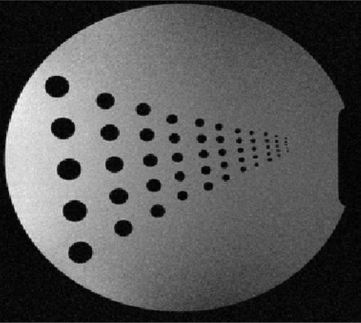
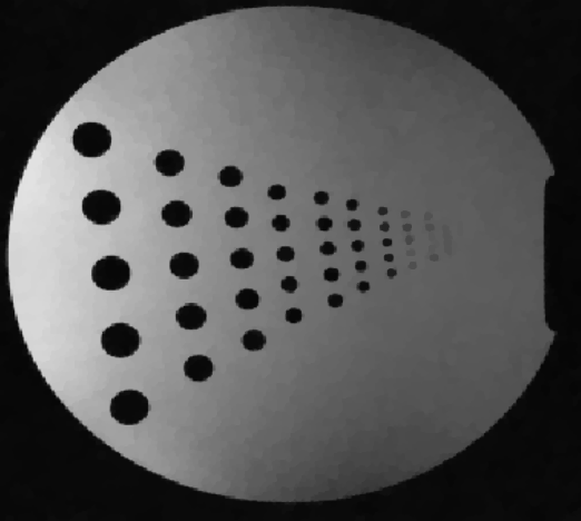
	$\lambda_{1}=0.6$	$\lambda_{2}=0.004$
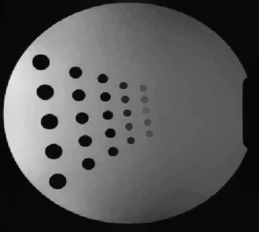
	$\lambda_{1}=0.3$	$\lambda_{2}=0.002$

Figure 3: Denoising with $\operatorname{KR}$-$\operatorname{TV}$ and $L^{1}$-$\operatorname{TV}$. In the right images $\lambda_{1}$ is so large that the respective constraint is inactive.

In Figure 4 we took a piecewise affine image, contaminated by noise and denoised it by $L^{1}$-$\operatorname{TV}$ and $\operatorname{KR}$-$\operatorname{TV}$. The parameters $\lambda_{1}$, respectively $\lambda_{2}$ have been tuned by hand to give a minimal $L^{1}$-error to the ground truth, i.e. to the noise-free $u^{\dagger}$. Even though this choice seem to be perfectly suited for $L^{1}$-$\operatorname{TV}$ it turns out that $\operatorname{KR}$-$\operatorname{TV}$ achieves a smaller error. Also note that staircasing is slightly reduced but also edges are a little more blurred for $\operatorname{KR}$-$\operatorname{TV}$ than for $L^{1}$-$\operatorname{TV}$.

	$u^{\dagger}$
noisy, $u^{0}$	$L^{1}$-TV	KR-TV
	$\|u-u^{\dagger}\|_{L^{1}}=295.7$	$\|u-u^{\dagger}\|_{L^{1}}=253.7$

Figure 4: Denoising with $\operatorname{KR}$-$\operatorname{TV}$ and $L^{1}$-$\operatorname{TV}$. Left: Noisy image, middle: KR-TV denoised by using the value $\lambda_{2}$ only ($\lambda_{1}$ so large, that the bound is inactive), right, $L^{1}$-TV denoising (i.e. only $\lambda_{1}$ is used). The respective values $\lambda_{1}$ and $\lambda_{2}$ have been optimized to result is the smallest $L^{1}$ error to the original noise-free image.

6.3 Cartoon-Texture decomposition

We compare the $\operatorname{KR}$-$\operatorname{TV}$ model for cartoon texture decomposition with $L^{1}$-$\operatorname{TV}$ and also with Meyer’s $G$-$\operatorname{TV}$ (cf. Section 4.3). In Figure 5 we show decompositions of Barbara into its cartoon and texture part. The parameters have been chosen as follows: We started with the value $\lambda_{1}$ for the $L^{1}$-$\operatorname{TV}$ decomposition (i.e. $\lambda_{2}=\infty$) and chose it such that most texture is in the texture component but also some structure is already visible. Then, for the $G$-$\operatorname{TV}$ the parameter was adjusted such that the cartoon part has the same total variation as the cartoon part from the $L^{1}$-$\operatorname{TV}$ decomposition. For the $\operatorname{KR}$-$\operatorname{TV}$ decomposition, the value $\lambda_{1}$ was set to $\infty$ while $\lambda_{2}$ was again chosen such that the total variation of the cartoon part equals the total variation of the other cartoon parts. The rationale behind this choice is, that the total variation is used as a prior for the cartoon part in all three models. We remark that the choosing the parameters such that the $L^{1}$-discrepancy of the texture part is equal for all three decompositions leads to slightly different, but visually comparable results.

Note that, for these parameters the $L^{1}$-$\operatorname{TV}$ decomposition already has some structure in the texture part (parts of the face and of the bookshelf) and the $G$-$\operatorname{TV}$ decomposition has structure and texture severely mixed, while for $\operatorname{KR}$-$\operatorname{TV}$ the texture component still mainly contains texture. Also note that $\operatorname{KR}$-$\operatorname{TV}$ manages to keep the smooth structure of the clothes in the cartoon part (see e.g. the scarf and the trousers) while $L^{1}$-$\operatorname{TV}$ gives a more “constant” cartoon image.

Original	$L^{1}$-$\operatorname{TV}$	$G$-$\operatorname{TV}$	$\operatorname{KR}$-$\operatorname{TV}$

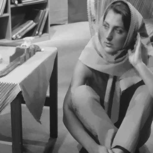
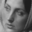
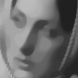
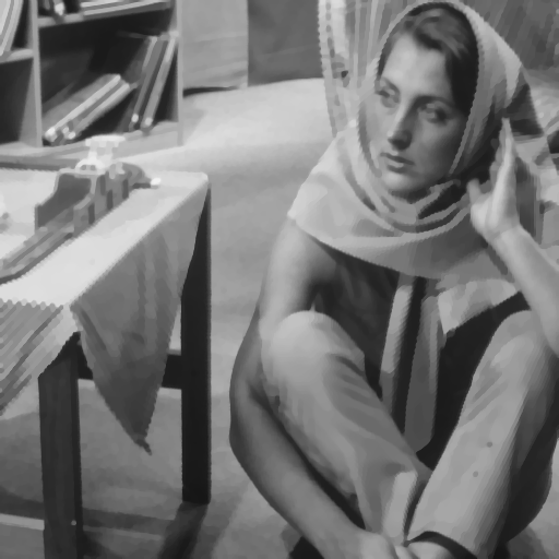
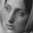
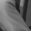
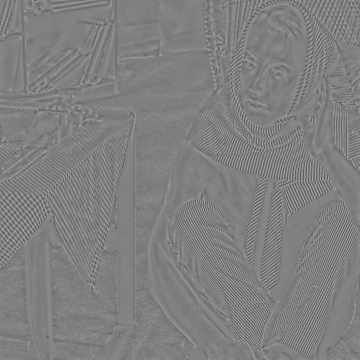
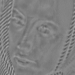
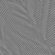
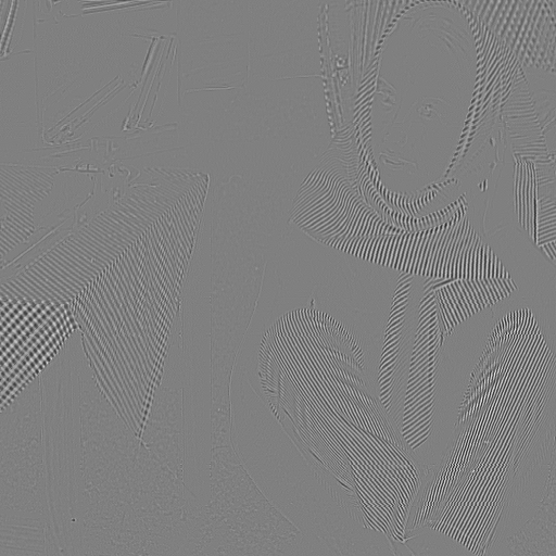
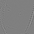
Figure 5: Cartoon-texture decomposition with $L^{1}$-$\operatorname{TV}$, $G$-$\operatorname{TV}$, and $\operatorname{KR}$-$\operatorname{TV}$. Top row: original and cartoon parts, bottom row: texture parts.

7 Conclusion

In this paper we propose a new discrepancy term in a total variation regularisation approach for images that is motivated by optimal transport. The proposed discrepancy term is the Kantorovich-Rubinstein transport norm. We show relations of this norm to other standard discrepancy terms in the imaging literature and derive qualitative properties of minimizers of a total variation regularization model with a KR discrepancy. Indeed, we find that the KR discrepancy can be seen as a generalization of the dual Lipschitz norm and the $L^{1}$ norm, both of which can be derived from the Kantorovich-Rubinstein norm by letting one of the parameters go to infinity, respectively. Moreover, we show that this specialization is in fact crucial for obtaining a model in which the solution conserves mass and that the model has a solution which preserves positivity.

The paper is furnished with a discussion of experiments where we use the $\operatorname{KR}$-$\operatorname{TV}$ regularisation approach in the context of image denoising and image decomposition. Our numerical discussion suggests that the use of the $\operatorname{KR}$ norm can reduce the $\operatorname{TV}$ staircasing effect and performs better when decomposing an image into a cartoon-like and oscillatory component. Due to the mass conversation property we also expect that this approach is interesting in medical imaging, where images are usually indeed density functions of physical quantities, as well as in the context of density estimation where total variation approaches have been used before in the context of earthquakes and fires, see [42] for instance. The applicability of the $\operatorname{KR}$ discrepancy in other imaging problems such as optical flow, image sequence interpolation or stereo vision has to be investigated in future research.

While some analytical properties of the $\operatorname{KR}$-$\operatorname{TV}$ method have been established (e.g. a weak maximum principle and a mass preservation property), a deeper understanding of the geometrical properties, as has been carried out for and $L^{1}$-$\operatorname{TV}$ and $L^{2}$-$\operatorname{TV}$, as well as for $\operatorname{TGV}$ on one-dimensional domains (see, e.g., [57, 13, 18, 8, 47, 49]), would indeed be interesting. However, due to the non-locality of the $\operatorname{KR}$ discrepancy, the analysis may be more complicated.

References

- [1] Luigi Ambrosio, Nicola Fusco, and Diego Pallara. Functions of bounded variation and free discontinuity problems, volume 254. Clarendon Press Oxford, 2000.
- [2] Luigi Ambrosio, Nicola Gigli, and Giuseppe Savaré. Gradient flows in metric spaces and in the space of probability measures. Lectures in Mathematics ETH Zürich. Birkhäuser Verlag, Basel, 2005.
- [3] Hedi Attouch and Haïm Brezis. Duality for the sum of convex functions in general Banach spaces. In Jorge Alberto Barroso, editor, Aspects of Mathematics and its Applications, volume 34 of North-Holland Mathematical Library, pages 125–133. Elsevier, 1986.
- [4] Jean-François Aujol, Guy Gilboa, Tony Chan, and Stanley Osher. Structure-texture image decomposition—modeling, algorithms, and parameter selection. International Journal of Computer Vision, 67(1):111–136, 2006.
- [5] V. I. Bogachev. Measure theory. Vol. I, II. Springer-Verlag, Berlin, 2007.
- [6] Doug M. Boyer, Yaron Lipman, Elizabeth St. Clair, Jesus Puente, Biren A. Patel, Thomas Funkhouser, Jukka Jernvall, and Ingrid Daubechies. Algorithms to automatically quantify the geometric similarity of anatomical surfaces. Proceedings of the National Academy of Sciences, 108(45):18221–18226, 2011.
- [7] Kristian Bredies, Karl Kunisch, and Thomas Pock. Total generalized variation. SIAM Journal on Imaging Sciences, 3(3):492–526, 2010.
- [8] Kristian Bredies, Karl Kunisch, and Tuomo Valkonen. Properties of -: The one-dimensional case. Journal of Mathematical Analysis and Applications, 398:438–454, 2013.
- [9] Kristian Bredies and Tuomo Valkonen. Inverse problems with second-order total generalized variation constraints. In Proceedings of the 9th International Conference on Sampling Theory and Applications (SampTA) 2011, Singapore, 2011.
- [10] Jonathan M. Bunn, Doug M. Boyer, Yaron Lipman, Elizabeth St. Clair, Jukka Jernvall, and Ingrid Daubechies. Comparing Dirichlet normal surface energy of tooth crowns, a new technique of molar shape quantification for dietary inference, with previous methods in isolation and in combination. American Journal of Physical Anthropology, 145(2):247–261, 2011.
- [11] Martin Burger, Marzena Franek, and Carola-Bibiane Schönlieb. Regularized regression and density estimation based on optimal transport. Applied Mathematics Research eXpress, 2012(2):209–253, 2012.
- [12] Giuseppe Buttazzo and Filippo Santambrogio. A model for the optimal planning of an urban area. SIAM J. Math. Anal., 37(2):514–530, 2005.
- [13] Vicent Caselles, Antonin Chambolle, and Matteo Novaga. The discontinuity set of solutions of the TV denoising problem and some extensions. Multiscale modeling & simulation, 6(3):879–894, 2007.
- [14] Antonin Chambolle and Thomas Pock. A first-order primal-dual algorithm for convex problems with applications to imaging. Journal of Mathematical Imaging and Vision, 40(1):120–145, 2011.
- [15] Tony F. Chan and Selim Esedoglu. Aspects of total variation regularized function approximation. SIAM Journal on Applied Mathematics, 65(5):1817–1837, 2005.
- [16] Tony F. Chan, Selim Esedoglu, and Kangyu Ni. Histogram based segmentation using Wasserstein distances. In Scale Space and Variational Methods in Computer Vision, pages 697–708. Springer, 2007.
- [17] Luigi De Pascale and Aldo Pratelli. Regularity properties for Monge transport density and for solutions of some shape optimization problem. Calculus of Variations and Partial Differential Equations, 14(3):249–274, 2002.
- [18] Vincent Duval, Jean-François Aujol, and Yann Gousseau. The TVL1 model: a geometric point of view. Multiscale Modeling & Simulation. A SIAM Interdisciplinary Journal, 8(1):154–189, 2009.
- [19] Vincent Duval, Jean-François Aujol, and LuminitaA. Vese. Mathematical modeling of textures: Application to color image decomposition with a projected gradient algorithm. Journal of Mathematical Imaging and Vision, 37(3):232–248, 2010.
- [20] Ivar Ekeland and Roger Temam. Convex analysis and variational problems. SIAM, 1999.
- [21] Herbert Federer. Geometric Measure Theory. Springer, 1969.
- [22] Sira Ferradans, Nicolas Papadakis, Julien Rabin, Gabriel Peyré, and Jean-François Aujol. Regularized discrete optimal transport. In Scale Space and Variational Methods in Computer Vision, pages 428–439. Springer, 2013.
- [23] Tom Goldstein, Ernie Esser, and Richard Baraniuk. Adaptive primal-dual hybrid gradient methods for saddle-point problems. arXiv preprint arXiv:1305.0546, 2013.
- [24] Michael Grant and Stephen Boyd. Graph implementations for nonsmooth convex programs. In V. Blondel, S. Boyd, and H. Kimura, editors, Recent Advances in Learning and Control, Lecture Notes in Control and Information Sciences, pages 95–110. Springer-Verlag Limited, 2008. http://stanford.edu/~boyd/graph_dcp.html.
- [25] Michael Grant and Stephen Boyd. CVX: Matlab software for disciplined convex programming, version 2.1. http://cvxr.com/cvx, March 2014.
- [26] Kristen Grauman and Trevor Darrell. Fast contour matching using approximate earth mover’s distance. In Computer Vision and Pattern Recognition, 2004. CVPR 2004. Proceedings of the 2004 IEEE Computer Society Conference on, volume 1, pages I–220. IEEE, 2004.
- [27] Steven Haker, Lei Zhu, Allen Tannenbaum, and Sigurd Angenent. Optimal mass transport for registration and warping. International Journal of Computer Vision, 60(3):225–240, 2004.
- [28] Leonid V. Kantorovič. On the translocation of masses. C. R. (Doklady) Acad. Sci. URSS (N.S.), 37:199–201, 1942.
- [29] Leonid V. Kantorovič and Gennadi Š. Rubinšteĭn. On a functional space and certain extremum problems. Doklady Akademii Nauk SSSR, 115:1058–1061, 1957.
- [30] Stefan Kindermann, Stanley Osher, and Jinjun Xu. Denoising by BV-duality. Journal of Scientific Computing, 28(2-3):411–444, 2006.
- [31] Haibin Ling and Kazunori Okada. An efficient earth mover’s distance algorithm for robust histogram comparison. Pattern Analysis and Machine Intelligence, IEEE Transactions on, 29(5):840–853, 2007.
- [32] Yaron Lipman and Ingrid Daubechies. Conformal Wasserstein distances: Comparing surfaces in polynomial time. Advances in Mathematics, 227(3):1047–1077, 2011.
- [33] Yaron Lipman, Jesus Puente, and Ingrid Daubechies. Conformal Wasserstein distance: II. Computational aspects and extensions. Math. Comput., 82(281):331–381, 2013.
- [34] Dirk A. Lorenz and Thomas Pock. An accelerated forward-backward algorithm for monotone inclusions. arXiv preprint arXiv:1403.3522, 2014.
- [35] Pertti Mattila. Geometry of sets and measures in Euclidean spaces: Fractals and rectifiability. Cambridge University Press, 1999.
- [36] Facundo Mémoli. On the use of Gromov-Hausdorff distances for shape comparison. In Eurographics symposium on point-based graphics, pages 81–90. The Eurographics Association, 2007.
- [37] Facundo Mémoli. Gromov-Hausdorff distances in euclidean spaces. In Computer Vision and Pattern Recognition Workshops, 2008. CVPRW’08. IEEE Computer Society Conference on, pages 1–8. IEEE, 2008.
- [38] Facundo Mémoli. Spectral Gromov-Wasserstein distances for shape matching. In Computer Vision Workshops (ICCV Workshops), 2009 IEEE 12th International Conference on, pages 256–263. IEEE, 2009.
- [39] Facundo Mémoli. Gromov-Wasserstein distances and the metric approach to object matching. Foundations of Computational Mathematics, 11(4):417–487, 2011.
- [40] Facundo Mémoli. A spectral notion of Gromov-Wasserstein distance and related methods. Applied and Computational Harmonic Analysis, 30(3):363–401, 2011.
- [41] Yves Meyer. Oscillating patterns in image processing and nonlinear evolution equations. American Mathematical Society, Providence, RI, 2001. The fifteenth Dean Jacqueline B. Lewis memorial lectures.
- [42] George O. Mohler, Andrea L. Bertozzi, Thomas A. Goldstein, and Stanley J. Osher. Fast TV regularization for 2D maximum penalized likelihood estimation. Journal of Computational and Graphical Statistics, 20(2):479–491, 2011.
- [43] Frank Morgan. Geometric Measure Theory: A Beginner’s Guide. Academic Press, 1987.
- [44] Kangyu Ni, Xavier Bresson, Tony F. Chan, and Selim Esedoglu. Local histogram based segmentation using the Wasserstein distance. International Journal of Computer Vision, 84(1):97–111, 2009.
- [45] Laurent Oudre, Jérémie Jakubowicz, Pascal Bianchi, and Chantal Simon. Classification of periodic activities using the Wasserstein distance. Biomedical Engineering, IEEE Transactions on, 59(6):1610–1619, 2012.
- [46] Nicolas Papadakis, Gabriel Peyré, and Edouard Oudet. Optimal transport with proximal splitting. SIAM Journal on Imaging Sciences, 7(1):212–238, 2014.
- [47] Konstantinos Papafitsoros and Kristian Bredies. A study of the one dimensional total generalised variation regularisation problem. arXiv preprint arXiv:1309.5900, 2013.
- [48] Gabriel Peyré, Jalal Fadili, and Julien Rabin. Wasserstein active contours. In Image Processing (ICIP), 2012 19th IEEE International Conference on, pages 2541–2544. IEEE, 2012.
- [49] Christiane Pöschl and Otmar Scherzer. Exact solutions of one-dimensional TGV. arXiv preprint arXiv:1309.7152, 2013.
- [50] Julien Rabin and Gabriel Peyré. Wasserstein regularization of imaging problems. In Image Processing (ICIP), 2011 18th IEEE International Conference on, pages 1541–1544. IEEE, 2011.
- [51] Julien Rabin, Gabriel Peyré, and Laurent D Cohen. Geodesic shape retrieval via optimal mass transport. In Computer Vision–ECCV 2010, pages 771–784. Springer, 2010.
- [52] Julien Rabin, Gabriel Peyré, Julie Delon, and Marc Bernot. Wasserstein barycenter and its application to texture mixing. In Scale Space and Variational Methods in Computer Vision, pages 435–446. Springer, 2012.
- [53] Svetlozar T. Rachev and Ludger Rüschendorf. Mass transportation problems. Vol. I. Probability and its Applications (New York). Springer-Verlag, New York, 1998. Theory.
- [54] Yossi Rubner, Carlo Tomasi, and Leonidas J Guibas. The earth mover’s distance as a metric for image retrieval. International Journal of Computer Vision, 40(2):99–121, 2000.
- [55] Bernhard Schmitzer and Christoph Schnörr. Modelling convex shape priors and matching based on the Gromov-Wasserstein distance. Journal of Mathematical Imaging and Vision, 46(1):143–159, 2013.
- [56] Bernhard Schmitzer and Christoph Schnörr. Object segmentation by shape matching with Wasserstein modes. In Energy Minimization Methods in Computer Vision and Pattern Recognition, pages 123–136. Springer, 2013.
- [57] David Strong and Tony Chan. Edge-preserving and scale-dependent properties of total variation regularization. Inverse Problems, 19(6):S165, 2003.
- [58] Paul Swoboda and Christoph Schnörr. Convex variational image restoration with histogram priors. SIAM Journal on Imaging Sciences, 6(3):1719–1735, 2013.
- [59] Luminita A Vese and Stanley J Osher. Modeling textures with total variation minimization and oscillating patterns in image processing. Journal of Scientific Computing, 19(1-3):553–572, 2003.
- [60] Cédric Villani. Optimal transport, volume 338 of Grundlehren der Mathematischen Wissenschaften [Fundamental Principles of Mathematical Sciences]. Springer-Verlag, Berlin, 2009. Old and new.
- [61] Wei Wang, John A. Ozolek, Dejan Slepcev, Ann B Lee, Cheng Chen, and Gustavo K. Rohde. An optimal transportation approach for nuclear structure-based pathology. Medical Imaging, IEEE Transactions on, 30(3):621–631, 2011.
- [62] Wotao Yin, Donald Goldfarb, and Stanley Osher. A comparison of three total variation based texture extraction models. Journal of Visual Communication and Image Representation, 18(3):240–252, 2007.
- [63] Lei Zhu, Yan Yang, Steven Haker, and Allen Tannenbaum. An image morphing technique based on optimal mass preserving mapping. IEEE Transactions on Image Processing, 16(6):1481–1495, 2007.