The lower bound on the precision of transcriptional regulation

Abstract

The diffusive arrival of transcription factors at the promoter sites on the DNA sets a lower bound on how accurately a cell can regulate its protein levels. Using results from the literature on diffusion-influenced reactions, we derive an analytical expression for the lower bound on the precision of transcriptional regulation. In our theory, transcription factors can perform multiple rounds of 1D diffusion along the DNA and 3D diffusion in the cytoplasm before binding to the promoter. Comparing our expression for the lower bound on the precision against results from Green’s Function Reaction Dynamics simulations shows that the theory is highly accurate under biologically relevant conditions. Our results demonstrate that, to an excellent approximation, the promoter switches between the transcription-factor bound and unbound state in a Markovian fashion. This remains true even in the presence of sliding, i.e. with 1D diffusion along the DNA. This has two important implications: (1) minimizing the noise in the promoter state is equivalent to minimizing the search time of transcription factors for their promoters; (2) the complicated dynamics of 3D diffusion in the cytoplasm and 1D diffusion along the DNA can be captured in a well-stirred model by renormalizing the promoter association and dissociation rates, making it possible to efficiently simulate the promoter dynamics using Gillespie simulations. Based on the recent experimental observation that sliding can speed up the promoter search by a factor of 4, our theory predicts that sliding can enhance the precision of transcriptional regulation by a factor of 2.

I INTRODUCTION

Biological cells regulate their protein levels by stimulating or repressing the expression of genes via the binding of transcription factors (TFs) to the regulatory sequences on the DNA called promoters. The fluctuations in the state of the promoter, switching between ‘on’ and ‘off’ due to the binding and unbinding of transcription factors, will propagate to the protein levels downstream. Because there are only very few transcription factors present in a cell and because they have to find their target site via a diffusive trajectory, these fluctuations are substantial. Furthermore, in contrast to what has been assumed before Hippel1989 , the binding of the TFs to their target is not diffusion limited Hammar2012a . This is likely to enhance the fluctuations in the promoter state even further.

The level of transcription is set by the fraction of time the promoter is in the ’on’ state. This fraction, in turn, is controlled by the TF concentration. But how well can the cell infer the TF concentration from the strongly fluctuating promoter occupancy? The diffusion and the limited affinity of the TF for the promoter puts a fundamental limit on how precise gene expression can be regulated. In turn, this puts a lower bound on the noise in gene expression.

Indeed, in a computational study by Van Zon et al. VanZon2006 , it was found that the diffusive arrival of TFs at the promoter is a major source of noise in gene expression. In their model, however, the promoter was represented as a sphere, and it was assumed that the transcription factors move by normal 3D diffusion on all length scales. However, it is now commonly believed that transcription factors find their promoter via a combination of 1D diffusion along the DNA and 3D diffusion in the cytoplasm Riggs1972 ; Richter1974 ; Hippel1989 ; Halford2004 ; Hu2006 ; Elf2007 ; Lomholt:2009vj ; Li2009 ; Hammar2012a .

Recently, it has been studied theoretically how deviations of the TFs transport from classical Brownian motion affects noise in gene expression Tkacik2009 ; Tamari2011 ; Kafri2012 . On length scales larger than the sliding distance, the transport process is essentially 3D diffusion, but on length scales smaller than the sliding distance, the dynamics is a complicated interplay of 3D diffusion in the cytoplasm and 1D diffusion on the DNA. This motivated Tkačik and Bialek to study a model in which TFs can move by 3D diffusion in the bulk, bind reversibly and non-specifically to DNA near the promoter, move by 1D diffusion along the DNA to the promoter, to which they can then bind specifically and reversibly Tkacik2009 . Tkačik and Bialek found that the effect of the larger target size on the noise in gene expression, provided by the 1D sliding along the DNA near the promoter, is largely canceled by the increased temporal correlations in 1D diffusion. As a result, sliding has, according to their analysis, only a small effect on the physical limits to the precision of transcriptional regulation.

Here we rederive the fundamental bound on the accuracy of transcriptional regulation. We study the same model as that of Tkačik and Bialek Tkacik2009 , but analyze it using the approach of Agmon, Szabo, and coworkers to study diffusion-influenced reactions Agmon1990 ; Kaizu2014 . Apart from one biologically motivated assumption and one mathematical approximation, this approach makes it possible to solve this model exactly. To test our theory, we have extended Green’s Function Reaction Dynamics VanZon2005A ; VanZon2005 ; VanZon2006 ; Takahashi2010 , which is an exact scheme for simulating reaction-diffusion systems at the particle level, to include 1D diffusion along cylinders. We find excellent agreement between the predictions of our theory and the simulation results.

Our expression for the sensing error differs qualitatively from that of Tkačik and Bialek Tkacik2009 . Our expression predicts that, as the average promoter occupancy approaches unity, the error diverges. This can be understood intuitively by noting that in this limit newly arriving TFs cannot bind the promoter, and hence no concentration measurements can be performed. We found the same result earlier for the binding of ligand to a spherical receptor Kaizu2014 .

The key ingredient that determines the lower bound on the accuracy of transcriptional regulation is the correlation time of the promoter state Berg1977 ; Bialek2005 ; Kaizu2014 . The correlation time is a complex function of the diffusion constants of the TFs in the cytoplasm and along the DNA, and the rates of non-specific DNA binding and specific promoter binding. However, we find that, to an excellent approximation, the promoter correlation time is that of a random telegraph process, in which the promoter switches between the TF bound and unbound state with effective rates that are constant in time. The reason is that in living cells, the TF concentration is typically low, i.e. in the nM range, while the sliding distance and sliding time are short, $\approx 50{\rm bp}$ and $<50{\rm ms}$, respectively Elf2007 ; Hammar2012a . As a result, even in the presence of sliding along the DNA, the time a TF spends near the promoter is short compared to the timescale on which TFs arrive at the promoter from the bulk, which is on the order of seconds to minutes Hammar2012a . Hence, a TF near the promoter either rapidly binds the promoter or rapidly escapes into the bulk. This makes it possible to integrate out the rapid promoter-TF rebindings and the unsuccessful TF bulk arrivals, and reduce the many-body, non-Markovian reaction-diffusion problem to a pair problem in which the TFs associate with and dissociate from the promoter with rates that are constant in time. These results underscore our earlier finding that the complex TF diffusion dynamics with its algebraic distributed waiting times can be described in a well-stirred model by renormalizing the association and dissociation rates. Importantly, this implies that this model can then be simulated using the Gillespie algorithmGillespie1977 ; VanZon2006 ; Kaizu2014 .

One of the most important implications of our observation that the promoter dynamics can be described by a random telegraph process, is that minimizing the promoter noise (correlation time) is equivalent to minimizing the time required for transcription factors to find and bind the promoter. As pointed out by Tkačik and Bialek, the combined system of 1D and 3D diffusion tends to have longer correlation times than the system with only 3D diffusion Tkacik2009 . However, the dominant effect is that the DNA binding increases the target size which speeds up the rate by which TFs find the promoter. Our results show that this decreases the promoter correlation time, which enhances the precision of transcriptional regulation, and lowers the noise in gene expression. This means that the large body of work on how proteins find their targets on the DNA Richter1974 ; Berg1981 ; Slutsky2004a ; Hu2006 ; Halford2004 ; Elf2007 ; Lomholt:2009vj ; Li2009 ; Hammar2012a could be used to study how cells can optimize the precision of transcriptional regulation. Our findings corroborate those of Hammar et al. Hammar2012a : the search time and hence the promoter noise (correlation time) can be minimized by optimizing the sliding time. The optimal sliding time depends on the probability that a TF which is in contact with the promoter will actually bind the promoter rather than sliding over it.

II THEORY

Following earlier work Berg1977 ; Bialek2005 ; Tkacik2009 ; Kaizu2014 , we imagine that the cell infers the average transcription factor concentration $\bar{c}$ from the promoter state $n(t)$ integrated over an integration time $T$, $n_{T}=(1/T)\int_{0}^{T}n(t)dt$. Here, $n(t)$ is one if at time $t$ a transcription factor is bound to the promoter, and zero otherwise. In the limit that the integration time $T$ is much longer than the correlation time $\tau_{n}$ of $n(t)$, the variance in our estimate $n_{T}$ of the true mean occupancy $\bar{n}$ is given by Berg1977 ; Kaizu2014

$$\left(\delta n\right)^{2}\equiv\sigma_{n,T}^{2}\simeq\frac{2\sigma_{n}^{2}\,\tau_{n}}{T}=\frac{P_{n}\left(\omega=0\right)}{T},\$$ (1)

where $\sigma_{n}^{2}=\langle{n^{2}}\rangle-\langle{n}\rangle^{2}$ is the variance of an instantaneous measurement, and $P_{n}(\omega)$ and $\hat{C}_{n}(s)$ are respectively the power spectrum and the Laplace transform of the auto-correlation function $C_{n}(t)$ of $n(t)$.

The uncertainty or expected error $\delta c$ in the corresponding estimate of the average concentration $\bar{c}$ is related to the error $\delta n$ in the estimate of $\bar{n}$ via the gain $d\bar{n}/d\bar{c}$,

$$\delta c=\left|\frac{d\bar{c}}{d\bar{n}}\right|\delta n.$$ (2)

Since the promoter is a binomial switch, the variance $\sigma_{n}^{2}=\bar{n}(1-\bar{n})$. Both the average occupancy $\langle{n}\rangle=\bar{n}$ and the gain $d\bar{n}/d\bar{c}$ are determined by the input-output relation $\bar{n}(\bar{c})$ and the average concentration $\bar{c}$, while the integration time $T$ is assumed given. Hence, to obtain the error in the concentration estimate, we need to know the promoter correlation time $\tau_{n}$.

We note that the above expressions are generic: they apply to all systems where the concentration is inferred from the binary binding state of a protein, be it a receptor on the membrane or a promoter. How the ligand molecules or the transcription factors diffuse to the receptor or the promoter only enters the problem via the magnitude of the receptor (promoter) correlation time.

II.1 Deriving the correlation function and correlation time

To derive the uncertainty $\delta n$ in our estimate of $\bar{n}$, we derive the correlation function for a binary switching process (see Eq. 1), following Kaizu et al. Kaizu2014 . We start with the general expression for the correlation function of a binary switch

$$C_{n}(\tau) \equiv \left\langle(n(\tau)-\bar{n})(n(0)-\bar{n})\right\rangle$$ (3)

$$= \bar{n}\left(p_{*|*}(\tau)-\bar{n}\right).$$ (4)

In the second line we introduced the probability that the promoter is bound at time $\tau$, given that is started in the bound state at $t=0$. This conditional probability is equal to

$$p_{*|*}(\tau)=1-\mathscr{S}_{\mathrm{rev}}(\tau|*)$$ (5)

where $\mathscr{S}_{\mathrm{rev}}(\tau|*)$ is the probability that the promoter is free at time $\tau$, given that it was bound initially. The promoter can undergo multiple rounds of binding and unbinding during the time $\tau$. We can describe this reversible process in terms of an irreversible one via the convolution Agmon1990

$$\mathscr{S}_{\mathrm{rev}}(t|*)=k_{-}\int_{0}^{t}[1-\mathscr{S}_{\mathrm{rev}}(t^{\prime}|*)]\mathscr{S}_{\mathrm{rad}}(t-t^{\prime}|z_{0})dt^{\prime}.$$ (6)

The first factor under the integral gives the probability that the promoter is occupied at time $t^{\prime}$. Then the transcription factor dissociates from the promoter with a rate $k_{-}$ and is placed in contact with the promoter on the DNA at position $z_{0}$. The second term under the integral, $\mathscr{S}_{\mathrm{rad}}(t-t^{\prime}|z_{0})$, gives the probability that the promoter remains unoccupied from the last dissociation up to time time $t$. Integrating over all intermediate times $t^{\prime}$, gives us the probability that the promoter is unoccupied at time $t$.

To solve Eq. 6, we need the irreversible survival probability of the promoter, $\mathscr{S}_{\mathrm{rad}}(t-t^{\prime}|z_{0})$. In general, this quantity cannot be analytically, since it depends on the history of binding events Agmon1990 ; Kaizu2014 . Following Agmon1990 ; Kaizu2014 , we will assume that after each promoter-TF dissociation event, the promoter with the TF at contact is surrounded by an equilibrium distribution of TFs. The survival probability is then given by

$$\mathscr{S}_{\mathrm{rad}}(t|z_{0})\simeq\mathscr{S}_{\mathrm{rad}}(t|{\mathrm{eq}})S_{\mathrm{rad}}(t|z_{0}),$$ (7)

where $\mathscr{S}_{\mathrm{rad}}(t|{\mathrm{eq}})$ is the survival probability of a promoter which is free initially and is surrounded by an equilibrium solution of TFs; $S_{\mathrm{rad}}(t|z_{0})$ is the probability that a free promoter with only a single TF at contact $z_{0}$ and no other TFs present, is still unbound at a later time $t$. Below, in sections II.3 and III.2, we discuss the validity of Eq. 7 in detail.

The quantity $\mathscr{S}_{\mathrm{rad}}(t|{\mathrm{eq}})$ can be found by solving the differential equation (App. A)

$$\frac{\partial\mathscr{S}_{\mathrm{rad}}(t|{\mathrm{eq}})}{\partial t}=-\bar{\xi}\,k_{\mathrm{rad}}(t)\,\mathscr{S}_{\mathrm{rad}}(t|{\mathrm{eq}}).$$ (8)

Here, $k_{\mathrm{rad}}(t)$ is the time-dependent rate coefficient, and, importantly, $\bar{\xi}$ is the average concentration of TFs on the DNA, and not the total concentration of TFs. The above equation relates the rate at which TFs that were in equilibrium at time $t=0$ bind the promoter at time $t$, $-\frac{\partial\mathscr{S}_{\mathrm{rad}}(t|{\mathrm{eq}})}{\partial t}$, to the rate at which TFs bind the promoter at time $t$ if it is not occupied, $\bar{\xi}\,k_{\mathrm{rad}}(t)$, times the probability that the promoter is indeed unoccupied, $\mathscr{S}_{\mathrm{rad}}(t|{\mathrm{eq}})$. Solving the equation yields

$$\mathscr{S}_{\mathrm{rad}}(t|{\mathrm{eq}})=e^{-\bar{\xi}\int_{0}^{t}k_{{\mathrm{rad}}}(t^{\prime})dt^{\prime}}.$$ (9)

Because the system obeys detailed balance, we can write $k_{{\mathrm{rad}}}(t)$ Agmon1990 as

$$k_{\mathrm{rad}}(t)=k_{+}\,S_{\mathrm{rad}}(t|z_{0}),$$ (10)

where $k_{+}$ is the intrinsic association rate of the TF when in contact with the promoter.

Before deriving the correlation function $C_{n}(\tau)$ in the Laplace domain, $\hat{C}_{n}(s)$, we give a relation which will prove useful. Namely, from Eqs. 8 and 10, it is clear that

$$\frac{\partial\mathscr{S}_{\mathrm{rad}}(t|{\mathrm{eq}})}{\partial t} = -\bar{\xi}k_{+}\,S_{\mathrm{rad}}(t|z_{0})\,\mathscr{S}_{\mathrm{rad}}(t|{\mathrm{eq}})$$ (11)

$$= -\bar{\xi}k_{+}\,\mathscr{S}_{\mathrm{rad}}(t|z_{0}).$$ (12)

To derive $\hat{C}_{n}(s)$, we first Laplace transform Eq. 6 and solve it for $\hat{\mathscr{S}}_{\mathrm{rev}}(s|*)$. By using the Laplace transformed Eqs. 4 and 12 and using that $k_{-}\bar{n}=k_{+}\bar{\xi}(1-\bar{n})$ and $\sigma^{2}_{n}=\bar{n}(1-\bar{n})$, we can express $\hat{C}_{n}(s)$ as a function of $\hat{\mathscr{S}}_{\mathrm{rad}}(s|{\mathrm{eq}})$ only (see also Kaizu2014 ):

$$\hat{C_{n}}(s)=\sigma_{n}^{2}\,\frac{\bar{n}\hat{\mathscr{S}}_{\mathrm{rad}}(s|{\mathrm{eq}})}{1-(1-\bar{n})s\hat{\mathscr{S}}_{\mathrm{rad}}(s|{\mathrm{eq}})}.$$ (13)

To obtain an analytically closed form for the correlation function, we require an expression for $\hat{\mathscr{S}}_{\mathrm{rad}}(s|{\mathrm{eq}})$. We use

$$\hat{\mathscr{S}}_{\mathrm{rad}}(s|{\mathrm{eq}})\simeq\frac{1}{s}\,\frac{1}{1+\bar{\xi}\hat{k}_{\mathrm{rad}}(s)},$$ (14)

which correctly captures the short- and long-time limit of $\mathscr{S}_{\mathrm{rad}}(t|{\mathrm{eq}})$ and becomes exact for all times in the low concentration limit Kaizu2014 . Substituting this approximation into Eq. 13, we obtain, after simplifying

$$\hat{C_{n}}(s)=\sigma_{n}^{2}\,\frac{\bar{n}}{\bar{n}s+k_{+}\bar{\xi}\,s\hat{S}_{\mathrm{rad}}(s|z_{0})}.$$ (15)

We can find the correlation time by taking the $s\to 0$ limit of the correlation function in Laplace space (see Eq. 1). Using that $\bar{n}=k_{+}\bar{\xi}/(k_{+}\bar{\xi}+k_{-})$, the expression for the correlation time of the promoter state becomes

$$\tau_{n}=\lim_{s\to 0}\frac{1}{\sigma_{n}^{2}}\hat{C}_{n}(s)=\frac{\tau_{c}}{S_{\mathrm{rad}}(\infty|z_{0})}.$$ (16)

Here $\tau_{c}=\left(k_{+}\bar{\xi}+k_{-}\right)^{-1}$ is the correlation time of the intrinsic switching dynamics, i.e. the correlation time of the promoter occupancy when the promoter-TF association is reaction-limited and the effect of diffusion can be neglected. Note that in geometries for which the particle always returns to the starting point, such as in 1D and 2D diffusion problems, $\lim_{t\to\infty}S_{\mathrm{rad}}(t|z_{0})\to 0$, such that the correlation time in Eq. 16 diverges. In these geometries, the particle always remains correlated with its starting point, and we are unable to define a correlation time. However, in the living cell, transcription factors do not only diffuse along the DNA, but also in the cytoplasm where memory is lost, yielding a finite correlation time.

In App. B we show that $S_{\mathrm{rad}}(\infty|z_{0})$ can be related to the intrinsic promoter-TF binding rate $k_{+}$ and the promoter-TF diffusion-limited association rate $k_{D}$. The latter is defined as the rate at which TFs, starting from an equilibrium distribution, arrive at (and instantly bind) the promoter. $k_{\rm D}$ is a complicated function of the diffusion speed of the TF in the cytoplasm and along the DNA, the rate of non-specific TF-DNA binding, the rate of TF-DNA dissociation and the TF-DNA binding cross-section. In terms of $k_{D}$ and $k_{+}$, the escape probability can be written as

$$S_{\mathrm{rad}}(\infty|z_{0})=\frac{k_{D}}{k_{+}+k_{D}}$$ (17)

which yields for the correlation time:

$$\tau_{n}=\frac{k_{+}+k_{D}}{(k_{+}\bar{\xi}+k_{-})k_{D}}.$$ (18)

In App. B we also show that the effective association rate $k_{\rm on}=k_{\rm rad}(t\to\infty)$ and the effective dissociation rate $k_{\rm off}$ are given by the diffusion-limited rate $k_{D}$ and the intrinsic binding and unbinding rates $k_{+}$ and $k_{-}$:

$$\frac{1}{k_{\mathrm{on}}} = \frac{1}{k_{+}}+\frac{1}{k_{\mathrm{D}}},$$ (19)

$$\frac{1}{k_{\mathrm{off}}} = \frac{1}{k_{-}}+\frac{K_{\mathrm{eq}}}{k_{\mathrm{D}}},$$ (20)

where $K_{\rm eq}\equiv k_{+}/k_{-}=k_{\rm on}/k_{\rm off}$ is the equilibrium constant. The correlation time can be expressed in terms of these rates as

$$\tau_{n}=\frac{1}{k_{\mathrm{on}}\bar{\xi}+k_{\mathrm{off}}}.$$ (21)

To summarize, once we have $k_{D}$, we can find from the expressions above the long-time limit of $S_{\mathrm{rad}}(t|z_{0})$, the effective association and dissociation rates $k_{\rm on}$ and $k_{\rm off}$, as well as the correlation time $\tau_{n}$. In section II.6 we show how we can obtain the diffusion-limited promoter association rate $k_{D}$ for a TF that can diffuse in the cytoplasm, slide along the DNA, and bind non-specifically to the DNA. The above analysis pertains, however, also to other problems in which signaling molecules have to bind a receptor molecule, possibly involving rounds of 3D, 2D or 1D diffusion; the different scenarios only yield different expressions for the diffusion-limited arrival rate of the signaling molecules at the receptor molecule, $k_{D}$.

II.2 The sensing error

Using the expression for the variance in our estimate of $\bar{n}$, Eq. 1, in combination with the result of Eq. 16, we find the general expression for the fractional error in our estimate of the promoter occupancy

$$\left(\frac{\delta n}{\bar{n}}\right)^{2}=2\,\frac{\sigma_{n}^{2}}{\bar{n}^{2}}\,\frac{\tau_{n}}{T}=2\,\frac{\sigma_{n}^{2}}{\bar{n}^{2}}\,\frac{\tau_{\mathrm{c}}}{S_{\mathrm{rad}}(\infty|z_{0})}\,\frac{1}{T}.$$ (22)

We combine equations Eq. 17 and Eq. 22 to find a general relation for the estimation error in terms of rate constants:

$$\left(\frac{\delta n}{\bar{n}}\right)^{2} = 2\bar{n}(1-\bar{n})\left[\frac{1}{\bar{n}k_{D}T\bar{\xi}}+\frac{1-\bar{n}}{k_{-}T\bar{n}^{2}}\right]$$ (23)

$$= \frac{2\sigma_{n}^{2}}{T\bar{\xi}\bar{n}}\,\frac{1}{k_{\mathrm{on}}},$$ (24)

where we have used that $\bar{n}k_{-}=(1-\bar{n})k_{+}\bar{\xi}$. A cell has to estimate the average TF concentration on the DNA, $\bar{\xi}$, from the average promoter occupancy $\bar{n}$. The fluctuations in the concentration estimate are related to the fluctuations in the promoter-occupancy estimate via

$$\delta\xi=\left|\frac{\partial\xi}{\partial n}\right|\delta n\quad\Rightarrow\quad\delta\xi=\frac{\bar{\xi}}{\bar{n}(1-\bar{n})}\delta n,$$ (25)

and therefore the error in the concentration inferred from the promoter state becomes

$$\left(\frac{\delta\xi}{\bar{\xi}}\right)^{2} = \frac{2}{\bar{n}(1-\bar{n})}\left(\frac{\bar{n}}{k_{D}T\bar{\xi}}+\frac{1-\bar{n}}{k_{-}T}\right)$$ (26)

$$= \frac{2}{T\bar{\xi}(1-\bar{n})}\,\frac{1}{k_{\mathrm{on}}}.$$ (27)

This expression has an intuitive interpretation: the fractional error in the concentration estimate decreases with the number of binding events during the integration time $T$, which is given by the number of binding events if the promoter were always free, $\bar{\xi}\,k_{\mathrm{on}}\,T$, times the fraction of time it is indeed free, $1-\bar{n}$.

To derive the error in the estimate of the concentration in the cytoplasm, we can exploit a detailed-balance relation for the TF concentration on the DNA, $\bar{\xi}$, and that in the cytoplasm, $\bar{c}$: $k_{d}\bar{\xi}=k_{a}\bar{c}$. Here, $k_{d}$ is the rate at which a TF dissociates from the DNA to which it was bound non-specifically, and $k_{a}$ is the rate at which it associates with the DNA (non-specifically). Using this relation, the expression for the fractional error in the cytoplasmic concentration estimate becomes

$$\left(\frac{\delta c}{\bar{c}}\right)^{2} = \frac{2}{\bar{n}(1-\bar{n})}\left(\frac{k_{d}}{k_{a}}\,\frac{\bar{n}}{k_{D}T\bar{c}}+\frac{1-\bar{n}}{k_{-}T}\right)$$ (28)

$$= \frac{2}{T\bar{c}(1-\bar{n})}\,\frac{k_{d}}{k_{a}}\,\frac{1}{k_{\mathrm{on}}}.$$ (29)

Lastly, we point out that the first term on the right-hand side of Eqs. 23,  26 and 28 gives the contribution to the sensing error from the finite speed of diffusion, while the second term gives the contribution from the intrinsic promoter switching dynamics.

II.3 The assumptions of our theory

Here we discuss the assumption, Eq. 7, and the approximation of our theory, Eq. 14, in more detail.

Eq. 7 states that after each TF dissociation event, the other TFs have the equilibrium distribution. By combining Eq. 1 and Eq. 13, it can be seen that this assumption implies that the correlation time of the promoter is given by

$$\tau_{n} = \bar{n}\hat{\mathscr{S}}_{\mathrm{rad}}(s=0|{\mathrm{eq}}),$$ (30)

$$= \bar{n}\tau_{\rm off}$$ (31)

where $\tau_{\rm off}=\int_{0}^{\infty}\mathscr{S}_{\mathrm{rad}}(t|{\mathrm{eq}})dt=\hat{\mathscr{S}}_{\mathrm{rad}}(s=0|{\mathrm{eq}})$ is the mean unbound time of a free promoter surrounded by TFs obeying the equilibrium distribution. The fact that the correlation time $\tau_{n}$ depends on the mean off time $\tau_{\rm off}$ and the mean occupancy $\bar{n}=\tau_{\rm on}/(\tau_{\rm on}+\tau_{\rm off})$ (and thus the mean on time $\tau_{\rm on}$), but not on the history of binding events, is a direct consequence of our assumption that after each TF dissociation event, the other TFs have the equilibrium distribution.

The mathematical approximation, Eq. 14, implies that $\tau_{\rm off}=\hat{\mathscr{S}}_{\mathrm{rad}}(s=0|{\mathrm{eq}})=1/(k_{\rm on}\bar{\xi})$. This is the mean waiting time for a Markov binding process with rate $k_{\rm on}\bar{\xi}$. While approximation Eq. 14 does not assume that binding is Markovian for all times, it does imply that in the relevant long-time limit binding occurs with a constant rate, yielding $\mathscr{S}_{\mathrm{rad}}(t|{\mathrm{eq}})=e^{-k_{\rm on}\bar{\xi}t}$.

Our theory predicts that the promoter correlation time $\tau_{n}$ is that of a two-state Markov state model, in which the switching events are independent, the waiting times are uncorrelated and exponentially distributed, and the promoter switches in a memoryless fashion with rates $k_{\rm on}\bar{\xi}$ and $k_{\rm off}$ that are constant in time. Therefore $\tau_{n}=(k_{\rm on}\bar{\xi}+k_{\rm off})^{-1}$. Below, we will see that that in the relevant long-time limit the promoter indeed switches in a Markovian fashion between the TF bound and unbound state.

II.4 Optimizing sensing precision by minimizing the search time

We now address the question whether the system can maximize the sensing precision by optimizing the strength of non-specific DNA binding, characterized by the equilibrium constant $K_{\rm eq}^{\rm ns}=k_{a}/k_{d}$. It is important to realize that the TF concentration in the cytoplasm, $\bar{c}$, and the TF concentration on the DNA, $\bar{\xi}$, are related via the detailed-balance relation $k_{a}\bar{c}=k_{d}\bar{\xi}$. This means that if were to fix $\bar{c}$, raising the DNA affinity $k_{a}/k_{d}$ would increase $\bar{\xi}$, and hence the total number of TFs in the system. This would trivially reduce the sensing error. The interesting question is whether there is an optimal DNA-binding strength that minimizes the sensing error for a fixed total number of TFs, $N$.

Since the TFs are either in the cytoplasm with a volume $L^{3}$, or nonspecifically bound to the DNA with a length $L_{\mathrm{D}}$, this yields the following constraint on the number of TFs:

$$N = \bar{c}L^{3}+\bar{\xi}L_{\mathrm{D}},$$ (32)

$$= \bar{c}(L^{3}+K_{\rm eq}^{\mathrm{ns}}L_{\mathrm{D}}),$$ (33)

where we have used that $\bar{\xi}=K_{\rm eq}^{\mathrm{ns}}\bar{c}$. Combining the above expression with Eq. 28 yields:

$$\frac{\delta c}{\bar{c}}=\sqrt{\frac{2}{T(1-\bar{n})}\,\frac{1}{k_{\mathrm{on}}}\,\frac{1}{N}\,\left(L_{\mathrm{D}}+\frac{L^{3}}{K_{\rm eq}^{\mathrm{n}s}}\right)}.$$ (34)

Because $N=\bar{c}(L^{3}+K_{\rm eq}^{\mathrm{ns}}L_{D})$, the expression on the right-hand side also gives the fractional error in the estimate of the total number of transcription factors, $\delta N/N$, and total TF concentration.

Interestingly, Eq. 34 shows that minimizing the sensor error at fixed promoter occupancy $\bar{n}$ is equivalent to minimizing the search time $\tau_{\mathrm{s}}$, which is the average time for a single TF to find the promoter starting from an equilibrium distribution:

$$\tau_{\mathrm{s}}=\frac{N}{\bar{\xi}\,k_{\mathrm{on}}}=\frac{1}{k_{\mathrm{on}}}\left(L_{\mathrm{D}}+\frac{L^{3}}{K_{\rm eq}^{\mathrm{ns}}}\right).$$ (35)

Indeed, the fractional error in the estimate of the number of transcription factors as a function of the search time is

$$\frac{\delta N}{N}=\sqrt{\frac{2\tau_{\rm s}}{N(1-\bar{n})T}}.$$ (36)

This is one of the central results of our paper. A system with a minimal search time, achieves a maximal rate of uncorrelated arrivals of TFs at the promoter. It is clear from our result in Eq. 34, that the sensing error and the gene expression noise coming from promoter-state fluctuations in such a system are minimal. The reason why minimizing the correlation time is equivalent to minimizing the search time is precisely that the promoter correlation time is that of a two-state Markov model, which is determined by the effective association rate $k_{\rm on}$ and effective dissociation rate $k_{\rm off}$, as discussed in the previous section.

II.5 Summary

Before we continue with our model of promoter-TF binding, we would like to remind the reader that we have made only one assumption up to this point, which is that after dissociation the dissociated TF is surrounded by an equilibrium solution of TFs (Eq. 7), and one approximation, namely that the Laplace transform of ${\mathscr{S}}_{\mathrm{rad}}(t|{\rm eq})$ is given by Eq. 14. We have made no assumptions on the geometry of the system yet, such that our expression for the correlation time and sensing precision hold for any geometry. The above theory applies to the binding of promoter-TF binding, involving 3D diffusion and 1D diffusion, but also to the binding of signaling molecules to proteins on the membrane, involving 3D and 2D diffusion. To obtain the correlation time and sensing precision in the different geometries, we need to find the long-time limit of the survival probability $S_{\mathrm{rad}}(\infty|z_{0})$ or the diffusion-limited on-rate for a single particle, $k_{D}$, in these different scenarios. Only one of these quantities suffices as both are related via Eq. 17. Deriving $S_{\mathrm{rad}}(\infty|z_{0})$ and $k_{D}$ for promoter-TF binding will be our main goal of the next section.

II.6 Model

We now derive the long-time limit of $S_{\mathrm{rad}}(t|z_{0})$, $S_{\mathrm{rad}}(\infty|z_{0})$, for the model shown in Fig. 1. The DNA near the promoter is described as a straight cylinder. In the cytoplasm TFs diffuse with diffusion constant $D_{3}$. A TF molecule can (non-specifically) bind DNA with an intrinsic association rate $k_{a}$ when it is in contact with it; the TF-DNA binding cross-section is $\sigma$. On the DNA, TFs can slide with diffusion constant $D_{1}$, dissociate into the cytoplasm with the intrinsic dissociation rate $k_{d}$, or, when they arrive at the promoter, bind the promoter with the intrinsic association rate $k_{+}$. A promoter-bound TF can dissociate from the promoter with rate $k_{-}$. We note that this model is identical to that Tkačik and Bialek Tkacik2009 . From $S_{\mathrm{rad}}(\infty|z_{0})$, we can obtain $k_{D}$, $k_{\rm on}$, $k_{\rm off}$, $\tau_{n}$, and the sensing error via Eqs. 17 - 21 and Eq. 28.

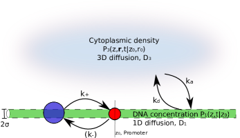
Figure 1: Model of TFs that can bind the promoter via 3D diffusion in the cytoplasm and 1D diffusion along the DNA. The DNA near the promoter is modeled as a straight cylinder. In the cytoplasm, the TFs diffuse with diffusion constant $D_{3}$. A single TF can associate with the DNA with the intrinsic association rate $k_{a}$ when it is in contact with it. On the DNA, a TF can slide with diffusion constant $D_{1}$, dissociate into the cytoplasm with the intrinsic dissociation rate $k_{d}$, or, when it arrives at the promoter, bind the promoter with rate $k_{+}$. A promoter-bound TF can dissociate from it with rate $k_{-}$. The diffusion along the DNA is described with the Green’s function $P_{1}(z,t|z_{0})$, and the diffusion inside the cytoplasm with $P_{3}(z,{\mathbf{r}},t|z_{0},r_{0})$. To derive $S_{\mathrm{rad}}(t|z_{0})$, we consider a single TF that starts at contact with the promoter, denoted by $z_{0}$. $S_{\mathrm{rad}}(t\to\infty|z_{0})$, the diffusion-limited binding rate $k_{D}$, the promoter correlation time $\tau_{n}$, and the sensing precision can be obtained via Eqs. 17 - 21 and Eq. 28.

To calculate $S_{\mathrm{rad}}(\infty|z_{0})$, we write down the full set of diffusion equations governing the behavior of a single TF starting on the promoter site:

$$\frac{\partial P_{1}(z,t|z_{0})}{\partial t} = D_{1}\frac{\partial^{2}P_{1}(z,t|z_{0})}{\partial^{2}z}-k_{d}P_{1}(z,t|z_{0})$$

$$-k_{+}P_{1}(z,t|z_{0})\delta(z-z_{0}) + k_{a}P_{3}(z,|{\mathbf{r}}|=\sigma,t|z_{0},r_{0})$$ (37)

$$\frac{\partial P_{3}(z,{\mathbf{r}},t|z_{0},r_{0})}{\partial t} = D_{3}\nabla^{2}P_{3}(z,{\mathbf{r}},t|z_{0},r_{0})$$

$$-\Big{[}k_{a}P_{3}(z,{\mathbf{r}},t|z_{0},r_{0}) - k_{d}P_{1}(z,t|z_{0})\Big{]}\frac{\delta(|{\mathbf{r}}|-\sigma)}{2\pi\sigma}.$$ (38)

Here $P_{1}(z,t|z_{0})$ is the Green’s function describing the 1D sliding of the TF along the DNA, starting at the promoter positioned at $z_{0}$. Excursions in the cytoplasm are described by $P_{3}(z,{\mathbf{r}},t|z_{0},r_{0})$, where $r_{0}=0$, stating that the particle starts on the DNA. We model the DNA as an infinitely long rod along the z-axis. Because the TF-DNA cross-section is $\sigma$, the probability exchange between the DNA and bulk happens at a distance $\sigma$ from the z-axis, imposed by the delta function in the second equation. In order to solve the equations, we first Laplace transform them with respect to time

$$s\,\hat{P}_{1}(z|z_{0})-\delta(z-z_{0}) = D_{1}\frac{\partial^{2}\hat{P}_{1}(z|z_{0})}{\partial^{2}z}-k_{+}\hat{P}_{1}(z|z_{0})\delta(z-z_{0})$$

$$- k_{d}\hat{P}_{1}(z|z_{0})+k_{a}\hat{P}_{3}(z,|{\mathbf{r}}|=\sigma|z_{0},r_{0})$$

$$s\,\hat{P}_{3}(z,{\mathbf{r}}|z_{0},r_{0}) = D_{3}\nabla^{2}\hat{P}_{3}(z,{\mathbf{r}}|z_{0},r_{0})$$

$$- \left[k_{a}\hat{P}_{3}(z,{\mathbf{r}}|z_{0},r_{0})-k_{d}\hat{P}_{1}(z|z_{0})\right]\frac{\delta(|{\mathbf{r}}|-\sigma)}{2\pi\sigma},$$

where we explicitly included the initial condition of one particle placed in contact with the promoter site on the DNA by the Dirac delta function. We continue by Fourier transforming with respect to space

$$s\,\tilde{P}_{1}(q|z_{0})-1 = -D_{1}q^{2}\tilde{P}_{1}(q|z_{0})-k_{+}\hat{P}_{1}(z_{0}|z_{0})$$

$$-k_{d}\tilde{P}_{1}(q|z_{0})+k_{a}\tilde{P}_{3}(q|z_{0},r_{0})$$

$$s\,\tilde{P}_{3}(q,{\mathbf{k}}|z_{0},r_{0}) = -D_{3}(q^{2}+k^{2})\tilde{P}_{3}(q,{\mathbf{k}}|z_{0},r_{0})$$

$$-\left[k_{a}\tilde{P}_{3}(q|z_{0},r_{0})-k_{d}\tilde{P}_{1}(q|z_{0})\right]J_{0}(k\sigma).$$

Here $q$ is the spatial Fourier variable conjugate to $z$, and ${\mathbf{k}}$ is conjugate to ${\mathbf{r}}$. $J_{0}(k\sigma)$ is the zeroth order Bessel function of the first kind. We take both the promoter and initial position to be at the origin: $z_{0}=0$. We want to solve these equations for $\tilde{P}_{1}(q|z_{0})$, from which we can extract the required survival probability $S_{\mathrm{rad}}(\infty|z_{0})$. Observe that the cytoplasmic density $\tilde{P}_{3}$ in Eq. II.6 is a function of $q$ only (and not of ${\mathbf{k}}$). In order to solve for $\tilde{P}_{1}$, we need an expression for $\tilde{P}_{3}(q|z_{0},r_{0})$ in terms of $\tilde{P}_{1}$. We start by solving the second equation for $\tilde{P}_{3}(q,{\mathbf{k}}|z_{0},r_{0})$,

$$\tilde{P}_{3}(q,{\mathbf{k}}|z_{0},r_{0})=\frac{k_{d}\tilde{P}_{1}(q|z_{0})-k_{a}\tilde{P}_{3}(q|z_{0},r_{0})}{s+D_{3}(q^{2}+k^{2})}J_{0}(k\sigma).$$ (41)

Fourier back-transforming both sides of the equation in ${\mathbf{k}}$, at $r=\sigma$, where we implicitly integrate over all ${\mathbf{r}}$,

$$\tilde{P}_{3}(q|z_{0},r_{0}) = \int d\nu\frac{\delta(r-\sigma)}{2\pi r}\tilde{P}_{3}(q,{\mathbf{k}}|z_{0},r_{0})$$

$$= \frac{k_{d}\tilde{P}_{1}(q|z_{0})-k_{a}\tilde{P}_{3}(q|z_{0},r_{0})}{2\pi D_{3}}\,I_{0}\left(\chi\right)K_{0}\left(\chi\right),$$

where $d\nu=\frac{d^{2}k}{(2\pi)^{2}}\mathrm{e}^{-i\,{\mathbf{k}}\cdot{\mathbf{r}}}$, $I_{0}$ and $K_{0}$ are the zeroth order modified Bessel functions of the first and second kind respectively, and $\chi=\sigma\sqrt{q^{2}+\frac{s}{D_{3}}}$. Solving the above for $\tilde{P}_{3}(q|z_{0},r_{0})$, and substituting the result into Eq. II.6, we obtain the solution for $\tilde{P}_{1}(q|z_{0})$. Again, back-transforming this equation in $q$ at the position of the promoter, $z_{0}=0$, we find

$$\hat{P}_{1}(z_{0},s|z_{0})=\int\frac{d\,q}{2\pi}\frac{1-k_{+}\hat{P}_{1}(z_{0},s|z_{0})}{s+D_{1}q^{2}+k_{d}F^{-1}(q,s)}$$ (43)

where

$$F(q,s)=1+\frac{k_{a}}{2\pi D_{3}}\,I_{0}\left(\chi\right)K_{0}\left(\chi\right).$$ (44)

Finally, we can solve Eq. 43 for $\hat{P}_{1}(z_{0},s|z_{0})$ to obtain the probability density at the promoter site in Laplace space. In the limit $s\to 0$, our expression becomes

$$\lim_{s\to 0}\hat{P}_{1}(z_{0},s|z_{0})=\frac{I(\alpha,\beta)}{\pi D_{1}/\sigma+k_{+}\,I(\alpha,\beta)}$$ (45)

where

$$I(\alpha,\beta) = \int_{0}^{\infty}\frac{dt}{t^{2}+\beta[1+\alpha\,I_{0}(t)K_{0}(t)]^{-1}}$$ (46)

$$\alpha = \frac{k_{a}}{2\pi D_{3}}$$ (47)

$$\beta = \frac{\sigma^{2}k_{d}}{D_{1}}.$$ (48)

To relate this result to the large time limit of the survival probability $S_{\mathrm{rad}}(\infty|z_{0})$, we exploit that the flux into the promoter at any given time is $k_{+}\,P_{1}(z_{0},t|z_{0})$, and that the total flux which leaks away through the promoter is equal to the integral over all times of the flux. Since the $s\to 0$ limit in the Laplace transformed function $\hat{P}_{1}(z_{0},s|z_{0})$ is exactly this integral, we find the survival probability via

$$\lim_{t\to\infty}S_{\mathrm{rad}}(t|z_{0}) = 1-k_{+}\,\int_{0}^{\infty}P_{1}(z_{0},t|z_{0})dt$$ (49)

$$= 1-k_{+}\lim_{s\to 0}\hat{P}_{1}(z_{0},s|z_{0})$$

$$= \frac{\frac{\pi D_{1}}{\sigma I(\alpha,\beta)}}{\frac{\pi D_{1}}{\sigma I(\alpha,\beta)}+k_{+}}.$$

Comparing with Eq. 17, the diffusion limited rate constant is

$$k_{D}=\frac{\pi D_{1}}{\sigma I(\alpha,\beta)}.$$ (50)

Plugging this result into Eqs. 23 and 28, the fractional error in the promoter-occupancy estimate is

$$\left(\frac{\delta n}{\bar{n}}\right)^{2}=2\bar{n}(1-\bar{n})\left[\left(\frac{\sigma I(\alpha,\beta)}{\bar{n}\pi D_{1}T\bar{\xi}}\right)+\frac{1-\bar{n}}{k_{-}T\bar{n}^{2}}\right],$$ (51)

and that in the cytoplasmic concentration $\bar{c}$ is

$$\left(\frac{\delta c}{\bar{c}}\right)^{2}=\frac{2}{\bar{n}(1-\bar{n})}\left(\frac{k_{d}}{k_{a}}\,\frac{\bar{n}\sigma I(\alpha,\beta)}{\pi D_{1}T\bar{c}}+\frac{1-\bar{n}}{k_{-}T}\right).$$ (52)

In the limit that DNA binding is reaction limited, $k_{a}\ll D_{3}$, it is very unlikely that the TF will rebind with the DNA after falling off, and the cytoplasm becomes effectively well mixed. In this limit, $\alpha\to 0$ in the integral of Eq. 46, and we can analytically solve it. The diffusion limited on-rate to the promoter becomes in this limit

$$k_{D}=\sqrt{4D_{1}k_{d}}=\sqrt{2}bk_{d},$$ (53)

where $b=\sqrt{2D_{1}/k_{d}}$ is the average length of a single excursion along the DNA. This equation has an intuitive interpretation. On average, a TF binding the DNA within a distance $\sim b$ from the promoter site, will find it. The rate at which molecules leave the DNA from this region is $~{}\sim bk_{d}\bar{\xi}$. Because our system obeys detailed balance, this rate of departure equals the rate of arrival, $k_{D}\bar{\xi}$, hence $k_{D}\sim bk_{d}$.

III RESULTS

III.1 Comparing theory with simulations

To test our theory, we have performed simulations using the enhanced Green’s Function Reaction Dynamics algorithm (GFRD) Takahashi2010 . Recently, we have expanded the functionality of GFRD  to simulate diffusion and reactions on a plane (2D) and along a cylinder (1D). Particles can exchange between the bulk and planes or cylinders via association and dissociation. Furthermore, specific binding sites can be added to a cylinder to which a particle diffusing along the cylinder can bind. Importantly, GFRD, is an exact scheme for simulating reaction-diffusion problems at the particle level, making it ideal to test theoretical predictions.

Parameter	Value	Motivation
$L$	1 $\upmu{\rm m}$	Bacterium size
$L_{\mathrm{D}}$	1 mm	E. Coli DNA length
$\mathrm{TF}_{0}$	10	Elf2007
$D_{1}$	5 $10^{-2}$ $\upmu{\rm m^{2}/s}$	Elf2007
$D_{3}$	3 $\upmu{\rm m^{2}/s}$	Elf2007
$k_{a}$	1 $\upmu{\rm m^{2}/s}$	Tabaka2014
$k_{d}$	1000/s	Elf2007 ; Tabaka2014
$k_{+}$	Varies	-
$k_{-}$	100/s in Fig. 2 and Fig. 3	-
	Varies in Fig. 4 and Fig. 5	Such that $\bar{n}=0.5$
$\sigma$	4 nm	-
$T$	100 s	-

Table 1: Typical values of the parameters used in our simulations and figures. When different values for the parameters are used, they are given in the text or figure captions.

Our simulation setup consist of a box with periodic boundary conditions. To model the DNA, the box contains a cylinder, which crosses the box. The promoter is modeled as a specific binding site at the middle of the cylinder. The box contains 10 transcription factors. Other details, such as parameter values, are given in Table. 1. We record the trajectory of the promoter, switching between the occupied and unoccupied state, for a period of 3000 seconds.

The key quantity of our theory is the zero-frequency limit of the power spectrum, $\lim_{\omega\to 0}P_{n}(\omega)=2\sigma^{2}_{n}\tau_{n}$, since the uncertainty in the promoter-occupancy and the concentration estimate can be directly obtained from this quantity and the gain (see Eq. 1 and Eq. 2). We therefore take the power spectrum of the promoter signal, following the procedure described in VanZon2006 .

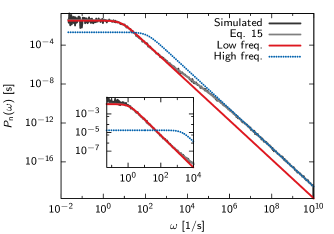
Figure 2: The power spectrum of the promoter state $P_{n}(\omega)$, for $\bar{n}=0.14$. The simulation results (black line) agree well with the theoretical prediction (Eq. 15). At high frequencies, the effect of diffusion is negligible and the promoter dynamics is that a Markovian switching process with intrinsic rates $k_{+}\bar{\xi}$ and $k_{-}$ (blue dotted line). At low frequencies, promoter switching can again be described by a random telegraph process, but now with effective rates $k_{\rm on}\bar{\xi}$ and $k_{\rm off}$ (red solid line). The association rate $k_{+}=0.16\mathrm{mm/s}$ and other parameters as given in Table Table. 1. The inset shows a power spectrum for a higher association rate $k_{+}=19\mathrm{mm/s}$ where $\bar{n}=0.67$.

Fig. 2 shows that the agreement between theory and simulations is very good over essentially the full frequency range, as observed previously for the binding of ligand to a spherical receptor Kaizu2014 . In the high-frequency regime, diffusion hardly plays any role and the receptor dynamics is dominated by the binding of TF molecules that are essentially in contact with the promoter; consequently, the power spectrum is well approximated by that of a binary switching process with uncorrelated exponentially distributed waiting times with the intrinsic correlation time $\tau_{c}=(k_{+}\bar{\xi}+k_{-})^{-1}$ (blue dotted line). The theory also accurately describes the intermediate frequency regime, in which a dissociated TF molecule manages to diffuse away from the promoter, but then rebinds it before another TF molecule does. The low frequency regime of the power spectrum corresponds to the regime in which after promoter dissociation the TF molecule diffuses into the bulk and, most likely, another TF molecule from the bulk binds the promoter. In this regime, the spectrum is well approximated by that of a memoryless switching process with the same effective correlation time as that of our theory, $\tau_{n}=(k_{\rm on}\bar{\xi}+k_{\rm off})^{-1}$ (solid red line).

Fig. 3 shows the zero-frequency limit of the power spectrum, $P_{n}(\omega\to 0)$, as a function of the the average occupancy $\bar{n}$, where we change $\bar{n}$ by varying the intrinsic association rate $k_{+}$. The theory matches simulation very well up to $\bar{n}\sim 0.8$. For higher value’s of $\bar{n}$, it is harder to measure the plateau value at the low frequency limit of the power spectrum, as shown in the inset of Fig. 2.

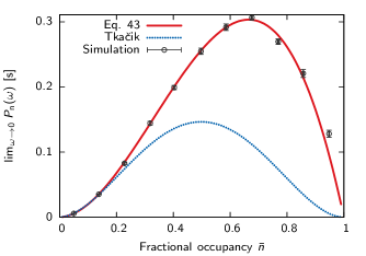
Figure 3: The low frequency limit of the power spectrum given by Eq. 1 as a function of the average occupancy $\bar{n}$ (red line), is in excellent agreement with simulation results. The dashed (blue) line shows the low frequency limit as derived in Tkacik2009 , which is symmetric in $\bar{n}$. $\bar{n}$ is varied by varying $k_{+}$. Other parameters are given in Table. 1.

III.2 Why the theory is accurate: timescale separation

The key assumption of our theory is Eq. 7, which states after each TF-promoter dissociation event, the other TFs have the equilibrium distribution. This assumption breaks down when two conditions are met: a) the rebinding of a TF to the promoter is pre-empted by the binding of a second TF from the bulk; and b) when the second TF dissociates from the promoter before the first has diffused in the bulk Kaizu2014 . We now consider both conditions.

In E. coli, the time required for a lac repressor molecule to bind the promoter from the bulk is on the other of seconds to minutes Hammar2012a . The time a dissociated repressor molecule spends near the promoter is on the order of the sliding time, which is $1-100{\rm ms}$ Elf2007 ; Marklund2013 . This timescale separation means that the likelihood that a TF from the bulk pre-empts the rebinding of a dissociated TF to the promoter is negligible; the probability of rebinding interference is very low and a dissociated TF rebinds the promoter before escaping into the bulk as often as when it would be the only TF in the system. This means that condition a) is not satisfied, and hence the assumption of Eq. 7 holds.

Even if there is occasionally rebinding interference, then Eq. 7 still probably holds because condition b) is not met. To determine whether a TF dissociates from the promoter before the previously dissociated TF has escaped into the bulk, we compare $k_{-}^{-1}$, the time a TF is specifically bound to the promoter, to the time a TF resides on the DNA (bound non-specifically) before escaping into the bulk. We can estimate the intrinsic dissociation time $k_{-}$ from the specific dissociation constant $K_{D}^{s}=k_{d}k_{-}/(k_{+}k_{a})$ and from $k_{d}$, $k_{+}$ and $k_{a}$. The microscopic non-specific binding rate for the lac repressor has been estimated to be $k_{i}\approx 3\times 10^{5}{\rm M^{-1}s^{-1}}$ Tabaka2014 . This yields $k_{a}=k_{i}/d\approx 1\mu{\rm m^{2}/s}$, where $d=0.3{\rm nm}$ is the distance between DNA base pairs. The specific promoter association rate $k_{+}$ can be estimated from $k_{+}=\gamma D_{1}/d$, which with $\gamma=0.1$ Hammar2012a and the 1D diffusion constant $D_{1}=0.05\mu{\rm m}^{2}/{\rm s}$ Elf2007 , yields $k_{+}\approx 10\mu{\rm m/s}$. The DNA dissociation rate for the lac repressor is $k_{d}\approx 10-1000/{\rm s}$ Elf2007 ; Marklund2013 . The dissociation constant for repressor binding to the operator $O_{1}$ is in the nM regime Riggs1970 . Taken together, these numbers imply that the time the repressor is bound for a time $k_{-}^{-1}$ that is at least seconds. This is consistent with the experimental observation of Hammar et al. that individual operator-bound LacI molecules appear as diffraction-limited spots on a $4{\rm s}$ timescale Hammar2012a . This is longer than our estimate for how long a TF which has dissociated from the promoter, resides near the promoter before escaping into the bulk, which is $1-100{\rm ms}$ Elf2007 ; Marklund2013 . We thus conclude that also condition b) is not satisfied; even if rebindings occur and condition a) is met, the central assumption of our theory, Eq. 7, will thus hold.

The principal reason why the key assumption Eq. 7 holds, is thus that the time TFs spend near the promoter is very short, both on the timescale at which TFs arrive at the promoter from the bulk and on the timescale a TF is bound to the promoter.

That TFs spend little time near the promoter as compared to the time required to bind the promoter from the bulk, is also the reason why the mathematical approximation, Eq. 14, is very accurate. In this approximation, $\mathscr{S}_{\mathrm{rad}}(t|{\mathrm{eq}})=e^{-\bar{\xi}k_{\rm on}t}$ at long times. The range over which $\mathscr{S}_{\mathrm{rad}}(t|{\mathrm{eq}})=e^{-\bar{\xi}\int_{0}^{t}dt^{\prime}k_{\rm rad}(t^{\prime})}$ deviates from this long-time limit is determined by how rapidly $S_{\rm rad}(t|z_{0})$ decays (because that determines how fast $k_{\rm rad}(t)$ reaches its long-time limit $k_{\rm on}$, see Eq. 10). This decay is dominated by $k_{d}$, which is at least an order of magnitude faster than the long-time decay governed by $k_{\rm on}\bar{\xi}$. Hence, after a promoter dissociation event, the dissociated TF essentially instantly rebinds the promoter or instantly escapes into the bulk, and then (most likely) another TF binds the promoter in a memoryless fashion, with a constant rate $k_{\rm on}\bar{\xi}$.

III.3 Comparison with Tka$\check{\mathbf{c}}$ik and Bialek

The sensing precision was derived earlier by Tka$\check{\mathrm{c}}$ik and Bialek, but via a different method Tkacik2009 . They start with the differential equations governing the fluctuations in the promoter state $\delta n$, and relate these to changes in the free energy due to the binding and unbinding of TFs. The fluctuations in the occupancy are then related to the power spectrum via the fluctuation-dissipation theorem.

Their final result for the noise in the promoter state is (Eq. 68 in Tkacik2009 )

$$\left(\frac{\delta n}{\bar{n}}\right)^{2}=2\bar{n}(1-\bar{n})\left[(1-\bar{n})\,\frac{\sigma I(\alpha,\beta)}{\bar{n}\pi^{2}D_{1}T\bar{\xi}}+\frac{1-\bar{n}}{k_{-}T\bar{n}^{2}}\right]$$ (54)

where $I(\alpha,\beta)$ is given by

$$I(\alpha,\beta)=\int_{0}^{\infty}\frac{dt}{t^{2}+\beta[1+\alpha\,{\mathrm{log}}(1+t^{-2})]^{-1}},$$ (55)

and $\alpha=k_{a}/(4\pi D_{3})$ and $\beta=k_{d}\sigma^{2}/(\pi D_{1})$.

The most important difference is the extra factor $(1-\bar{n})$ in the diffusion term, which makes $P_{n}(\omega\to 0)$ symmetric around $\bar{n}=0.5$, as is shown in Fig. 3 (blue dotted line). Our simulations results in Fig. 3 show however, that the maximum is reached when the promoter is occupied for more than half of the time.

Furthermore, in contrast to our result in Eq. 52, the precision of the TF concentration estimate (Eq. 71 in Tkacik2009 ) is independent of the promoter occupancy $\bar{n}$. However, since incoming TFs can not bind with the promoter when it is already occupied, it becomes harder to perceive the TF concentration as the promoter occupancy increases. In other words, the number of independent ‘measurements’ the promoter can make of the TF concentration during its integration time $T$, decreases with increasing occupancy. As a result, one would expect the noise to diverge as $\bar{n}\to 1$. Kaizu et al. Kaizu2014 obtained precisely the same discrepancy for a spherical receptor. The extra $(1-\bar{n})$ factor in Eq. 54 is most likely the result of a linearizion Tkacik2009 ; Kaizu2014 .

III.4 A coarse-grained model

In previous work, we have shown that the effect of TF diffusion in a spatially resolved model of promoter-TF binding can be captured in a well-stirred model by renormalizing the association and dissociation rates VanZon2006 ; Kaizu2014 . The principal observation is that a TF molecule near the promoter either rapidly binds the promoter or rapidly escapes into the bulk, as discussed in section III.2. As a consequence, the probability that the binding of this molecule to the promoter is pre-empted by the binding of another ligand molecule, is negligible: a TF molecule near the promoter binds the promoter or escapes into the bulk with splitting probabilities that are the same as when it would be the only TF molecule in the system. There is no (re)binding interference. This makes it possible to integrate out the rapid rebindings and the unsuccessful bulk arrivals, and reduce the complicated many-body reaction-diffusion problem to a pair problem in which ligand molecules interact with the receptor in a memory-less fashion, with renormalized association and dissociation rates. However, in these previous studies, the receptor (the promoter) was modeled as a sphere. While in VanZon2006 we predicted that rebindings could also be integrated out in a more detailed model of gene expression in which TFs do not only diffuse in the cytoplasm but also slide along the DNA, this question has so far not been answered. Here, we show that the answer is positive.

When the probability of rebinding interference is negligible, the effective dissociation rate $k_{\mathrm{off}}$ is given by VanZon2006 ; Kaizu2014 :

$$k_{\mathrm{off}}=\frac{k_{-}}{1+N_{\mathrm{reb}}}.$$ (56)

Here $N_{\mathrm{reb}}$ is the average number of rebindings, which is defined as the average number of rounds of rebinding and dissociation before a dissociated TF escapes into the bulk. It is given by

$$N_{\mathrm{reb}}=\sum_{n=1}^{\infty}n\left(p_{\mathrm{reb}}\right)^{n}p_{\mathrm{esc}}=\frac{1-p_{\mathrm{esc}}}{p_{\mathrm{esc}}},$$ (57)

where $p_{\mathrm{reb}}$ and $p_{\mathrm{esc}}=1-p_{\mathrm{reb}}$ are the splitting probabilities of a TF at contact for either rebinding the promoter or escaping into the bulk. The probability of a TF escaping is given by the $t\to\infty$ limit of the survival probability of a particle starting at contact

$$p_{\mathrm{esc}}=\lim_{t\to\infty}S_{\mathrm{rad}}(t|z_{0})=S_{\mathrm{rad}}(\infty|z_{0}).$$ (58)

Combining the above expressions, we find that $k_{\rm off}$ is precisely the effective dissociation rate of our theory, Eq. 20.

When the probability of rebinding interference is negligible, the effective association rate $k_{\rm on}$ is the rate at which a TF arrives from the bulk at the promoter, $k_{D}$, times the probability $1-S_{\mathrm{rad}}(\infty|z_{0})=k_{+}/(k_{+}+k_{D})=p_{\rm reb}$ (see Eq. 17) that it subsequently binds Kaizu2014 :

$$k_{\rm on}=\frac{k_{+}k_{D}}{k_{+}+k_{D}}.$$ (59)

This indeed is the effective association rate of our theory, Eq. 19. Again we see that the complicated dynamics of 3D diffusion, 1D sliding, and exchange between cytoplasm and DNA, is contained in the arrival rate $k_{D}$ and the escape probability $S_{\mathrm{rad}}(\infty|z_{0})$, which are related via Eq. 17.

This picture yields the simple two-state model:

$$\frac{dn(t)}{dt}=k_{\rm on}\bar{\xi}(1-n(t))-k_{\rm off}n(t).$$ (60)

In this model, the promoter switches with exponentially distributed waiting times between the on and the off state, with a correlation time which is precisely that of our theory, Eq. 21. As Fig. 3 shows, even in the presence of 1D diffusion along the DNA, this two-state model accurately describes the zero-frequency limit of the power spectrum, which determines the promoter correlation time and hence the sensing precision. The main reason why sliding does not change our earlier result obtained for a spherical promoter VanZon2006 is that the non-specific residence time on the DNA, $<50{\rm ms}$, Elf2007 ; Marklund2013 , is small compared to the timescale of seconds to minutes on which TFs bind the promoter from the bulk Hammar2012a , see section III.2.

III.5 Optimizing the sensing precision

We now minimize the sensing error keeping the average promoter occupancy constant at $\bar{n}=0.5$. The volume of the box is approximately that of a bacterium such that, $L=1\mathrm{\mu m}$, and for the length of the DNA we take the typical value $L_{\mathrm{D}}=1\mathrm{mm}$.

In Fig. 4 we plot the sensing error as a function of the DNA dissociation rate $k_{d}$. Different lines correspond to different values of the intrinsic promoter association rate $k_{+}$. In these calculations, we fix $D_{3}$, $D_{1}$, and $k_{a}$, and adjust $k_{-}$ such that $\bar{n}=0.5$. It is seen that there is an optimal dissociation rate $k_{d}$ and hence an optimal affinity $K_{\rm eq}^{\rm ns}=k_{a}/k_{d}$ that minimizes the sensing error. Tkačik and Bialek did not find an optimum, because they did not constrain the total number of TFs to be constant Tkacik2009 .

Finding the promoter involves rounds of 1D diffusion along the DNA and 3D diffusion in the cytoplasm Hippel1989 . The optimal search time is due to a trade-off between how long each round takes and the number of rounds $M$ needed to find the promoter Hippel1989 ; Slutsky2004a ; Hu2006 . The total search time is $\tau_{s}=M(\tau_{1D}+\tau_{3D}$), where $\tau_{3D}$ is the time a TF spends in the cytoplasm during one round and $\tau_{1D}$ is the time it spends on the DNA Slutsky2004a ; Hu2006 . The latter is given by $\tau_{1D}=1/k_{d}$. Ignoring correlations between the point of DNA dissociation and subsequent DNA association, $M\sim L_{D}/b$, where $b=\sqrt{2D_{1}/k_{d}}$ is the average length of a single excursion along the DNA. Hence, as $k_{d}$ is increased, $\tau_{1D}$ decreases as $1/k_{d}$, while $M$ increases as $\sqrt{k_{d}}$. This interplay leads to a minimum in the search time and hence the sensing error.

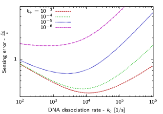
Figure 4: The sensing error (Eq. 34) as a function of the DNA dissociation rate $k_{d}$. The lines show the sensing error for different values of the intrinsic association rate of the promoter $k_{+}$, which are given in the legend and have units of m/s. The noise has an optimum when the search time of a TF for its target is the lowest. As we lower $k_{+}$, the sensing error increases because the TF has to arrive multiple times at the promoter before binding to it, which decreases the effective on-rate. We set the integration time $T$, which is usually the regulated protein lifetime, to $T=100$ s. When $k_{d}$ is varied, $k_{-}$ is tuned such that $\bar{n}=0.5$. Other parameters are fixed at typical biological values, given in Table. 1.

Slutsky and Mirny Slutsky2004a predicted that for an optimal search time, the TFs spend 50% of their time nonspecifically bound to the DNA and 50% in the cytoplasm. In their model, they assumed the cytoplasm to be well mixed ($D_{3}\to\infty$ in our model) and that the search process is diffusion limited, $k_{\mathrm{on}}\to k_{D}$. Recent experiments Hammar2012a , however, have shown that for some TFs the search process is not diffusion limited and that therefore the intrinsic association rate to the promoter $k_{+}$ will be similar or smaller than $k_{D}$. Furthermore, they show that a TF spends around 90% of its time nonspecifically bound to the DNA, much larger than predicted. Fig. 5 supports the proposition of Hammar2012a that these observations are related.

Fig. 5 shows the fraction of time a TF spends on the DNA, as a function of the association rate to the promoter $k_{+}$. It is reasonable to assume that transcriptional regulation operates in a parameter regime where the sensing error is low. Therefore, for each point in the figure, we chose $k_{d}$ such that the search time is minimal (minimum in Fig. 4). At high values of $k_{+}$, promoter binding becomes diffusion limited and thus independent of $k_{+}$. For lower values of $k_{+}$, however, the rate of promoter binding becomes increasingly limited by $k_{+}$. In this regime, the optimal fraction of time a TF spends on the DNA increases with decreasing $k_{+}$, rising to values above $50\%$. The reason is that, when $k_{+}$ is low, the TF needs to slide multiple times over the promoter before it binds, and this requires a more exhaustive search on the DNA for a minimal search time. This redundancy is enhanced by lowering $k_{d}$, which increases the DNA occupancy. Our results thus suggest that TFs spend more than 50% of their time on the DNA, because that minimizes the search time when promoter association is reaction limited.

Note that only in the case of a well mixed cytoplasm ($D_{3}\to\infty$, solid black line in Fig. 5, Eq. 53), the time a TF spends on the DNA converges to 50% as predicted by Slutsky and Mirny. For a finite cytoplasmic diffusion constant $D_{3}$, the fraction of time a TF is nonspecifically bound to the DNA is always lower than that in the well mixed case. As $D_{3}$ decreases, the probability that after DNA dissociation a TF will rapidly rebind the DNA instead of diffusing into the bulk, increases. This increases the average number of times $M^{\prime}$ a TF rapidly rebinds the DNA before it escapes into the bulk. Because a TF tends to rebind the DNA close to where it dissociated from it, rebindings increase the effective length $b_{\rm eff}$ of a DNA scan: $b_{\rm eff}=\sqrt{M^{\prime}}b$. To counter the effect of rebinding (increasing $M^{\prime}$) and to keep the effective scan length $b_{\rm eff}$ close to its optimal value, the rate of DNA dissociation $k_{d}$ has to be increased, so that $b$ is decreased. This lowers the fraction of time a TF spends on the DNA, as seen in Fig. 5.

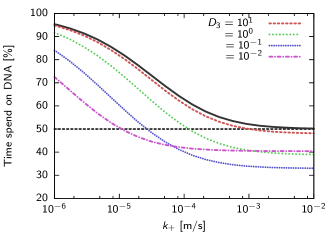
Figure 5: The fraction of time a TF spends on the DNA as a function of the intrinsic association rate to the promoter $k_{+}$. The DNA dissociation rate $k_{d}$ is chosen such that it minimizes the search time (minimum in Fig. 4). In a well mixed cytoplasm (solid black line), TFs spends the longest time on the DNA to minimize the search time, with a minimum of 50% as the search becomes diffusion limited at high rates of $k_{+}$. For finite cytoplasmic diffusion constants (colored dashed lines, values for $D_{3}$ are given in the legenda with units $\upmu{\rm m^{2}/s}$), the DNA occupancy is always lower because the spatial correlations of the TF with the DNA after dissociating from it, require a higher DNA dissociation rate $k_{d}$ for an optimal search speed. Also note that in the diffusion limited regime (high $k_{+}$), the curves converge to a DNA occupancy lower than 50%. Parameters: the promoter dissociation rate $k_{-}$ is always tuned such that $\bar{n}=0.5$. Other parameters are fixed at values given in Table. 1.

III.6 CONNECTION WITH PROMOTER NOISE IN GENE EXPRESSION

The fundamental bound on the precision of sensing TF concentrations puts a lower bound on the contribution to the noise in gene expression that comes from promoter-state fluctuations. Our observation that even in the presence of 3D diffusion and 1D sliding, the promoter switches to an excellent approximation in a Markovian fashion, makes it possible to quantify this “extrinsic” contribution.

Consider a gene which is expressed with a rate $\beta$ when a transcription factor is bound to its promoter. The expressed protein decays with a rate $\mu$. Our observation above shows that fluctuations in the promoter state $n(t)$ decay, to an excellent approximation, exponentially with a rate $\lambda$, corresponding to a promoter correlation time $\tau_{n}=\lambda^{-1}$. The noise in the protein copy number $X$ is then given by Paulsson2005 ; TanaseNicola2006

$$\sigma^{2}_{X} = \langle{X}\rangle+\left(\frac{\beta}{\mu}\right)^{2}\frac{\mu}{\mu+\lambda}\sigma_{n}^{2},$$ (61)

$$\equiv \sigma^{2}_{\rm in}+\sigma^{2}_{\rm ex}.$$ (62)

Here, $\sigma^{2}_{\rm in}=\langle{X}\rangle=(\beta/\mu)\langle{n}\rangle$ is the intrinsic noise in $X$; it would be the noise in $X$ if the state of the promoter were constant. The second term $\sigma^{2}_{\rm ex}$ describes the contribution to $\sigma_{X}^{2}$ from the fluctuations in the promoter state $n$. These fluctuations are amplified by the gain $g=\partial\langle{X}\rangle/\partial\langle{n}\rangle=\beta/\mu$, but integrated with an integration time given by the lifetime of the protein, $T=\mu^{-1}$ Paulsson2005 . When $T\gg\tau_{n}$, we can rewrite the above expression as

$$\sigma^{2}_{X}=\langle{X}\rangle+\left(\frac{\beta}{\mu}\right)^{2}\frac{\tau_{n}\sigma_{n}^{2}}{T}.$$ (63)

This expression highlights the idea that uncertainty in the estimate of $\bar{n}$, $\delta n=\sigma_{n_{T}}$, generates fluctuations in the expression level $X$, which are amplified by the gain $g$: $\sigma^{2}_{\rm ex}=g^{2}\sigma^{2}_{n_{T}}/2$. In fact, gene expression can be interpreted as a sampling protocol, in which the history of the promoter state $n(t)$ is stored in $X(t)$ Govern2013 . In this view, the copies of X constitute samples of $n(t)$. This perspective reveals that the factor 2 arises from the fact that the samples are degraded stochastically, which effectively increases the spacing between them Govern2013 .

IV DISCUSSION

We have rederived the fundamental bound on the precision of transcriptional regulation. To this end, we have developed a theory which is based on the model of promoter-TF binding put forward by Tkačik and Bialek Tkacik2009 . In this model, the DNA near the promoter is described as a straight cylinder. This seems reasonable since the sliding distance as measured experimentally, $\approx 50{\rm bp}$ Hammar2012a , is less than the persistence length of the DNA, which is on the order of $150{\rm bp}$. A TF that dissociates from the DNA, goes into the bulk where it moves by normal diffusion at all length scales. Here, we thus ignore the interplay between 3D diffusion, 1D sliding, hopping, and intersegmental transfer Berg1981 . However, at length scales larger than the sliding distance and the mesh length of the DNA polymer, the motion is essentially 3D diffusion. At these scales, TFs move with an effective diffusion constant, which is the result of diffusion in the cytoplasm, hopping, intersegmental transfer and sliding along the DNA Richter1974 ; Berg1981 ; Slutsky2004a ; Hu2006 ; Halford2004 ; Elf2007 ; Lomholt:2009vj ; Li2009 ; Hammar2012a . The diffusion constant $D_{3}$ in our model is indeed this diffusion constant.

It should be realized that even in our relatively simple model, promoter-TF binding is, in general, a complicated many-body non-Markovian problem, because rounds of promoter-TF association and dissociation can build up spatial-temporal correlations between the positions of the TF molecules Agmon1990 ; Kaizu2014 . Consequently, a free promoter is, in general, not surrounded by the equilibrium distribution of TF molecules, and the probability that a free promoter binds a TF will depend on the history of binding events. This impedes an exact solution of the problem.

However, following our earlier work Kaizu2014 , we can solve the problem almost analytically by making one assumption and one mathematical approximation. The assumption, Eq. 7, is that after each TF dissociation event, the other TFs have the equilibrium distribution. As a result, the probability that a free promoter binds a TF at a later time $t$, becomes independent of the history of binding events. The approximation is that the Laplace transform of $\mathscr{S}_{\mathrm{rad}}(t|{\mathrm{eq}})$ is given by Eq. 14. The assumption and approximation together mean that in our theory, the correlation time of the promoter is that of a random telegraph process, where the promoter switches between the TF bound and unbound states with rates that are constant in time.

We have tested our theory by performing particle-based simulations of the same model that underlies our theory. Because the GFRD algorithm is exact and the model is the same, all deviations between theory and simulations must be due to the assumption and/or approximation in the theory. To test the theory, we have computed the zero-frequency limit of the power spectrum, $P_{n}(\omega\to 0)=2\sigma^{2}_{n}\tau_{n}$, which is essentially a test of the correlation time $\tau_{n}$, because the variance $\sigma^{2}_{n}$ of a binary switch is given by the mean $\bar{n}$, $\sigma^{2}_{n}=\bar{n}(1-\bar{n})$. We find that $P_{n}(\omega\to 0)$ and hence the promoter correlation time is accurately predicted by our theory.

The success of our theory is rooted in the fact that the TF concentrations are typically low, the promoter-TF dissociation constant is (correspondingly) low, and the sliding time is short. As a result, the time a TF spends near the promoter is short on the timescale a TF is specifically bound to the promoter and on the timescale new TFs arrive from the bulk (see section III.2). A dissociated TF either rapidly rebinds the promoter, or rapidly escapes into the bulk. This means that the rebinding of a dissociated TF is typically not pre-empted by the binding of another TF from the bulk—there is no rebinding interference—which means that the central assumption of our theory, Eq. 7, holds. Because TFs spend little time near the promoter and because their concentration is low, also the mathematical approximation, Eq. 14, is very accurate.

Because TFs spend only little time near the promoter, promoter rebindings and unsuccessful bulk arrivals can be integrated out, and the complicated many-body non-Markovian problem can be reduced to a Markovian pair problem, in which TFs associate with and dissociate from the promoter with effective rates that are constant in time. The complicated dynamics of 3D diffusion and 1D sliding can thus be captured in a well-stirred model by renormalizing the association and dissociation rates. The off rate $k_{\rm off}$ is simply the intrinsic dissociation rate $k_{-}$ divided by the average number of bindings before escape (Eq. 56) and the on rate $k_{\rm on}$ is the bulk arrival rate $k_{D}$ times the binding probability. This probability is the inverse of the number of bindings (Eq. 59). This model can then be simulated using the Gillespie algorithm Gillespie1977 ; VanZon2006 ; Kaizu2014 . While our model does not take into account crowding, we expect that the same approach could be used in this case: the key observation is that inside the crowded environment of the cell, the time a TF spends near the promoter on the DNA is short compared to the time it is bound to the promoter and the time it takes to arrive at the promoter from the bulk Hammar2012a . This makes it possible to to study the effect of crowding on the dynamics of gene networks using a well-stirred model Morelli:2011ie .

An important consequence of the fact that the promoter dynamics can, to an excellent approximation, be described by a two-state Markov model is that the promoter correlation time is determined by the effective association and dissociation rates. This means that minimizing the sensing error, or the extrinsic noise in gene expression, at fixed promoter occupancy corresponds to minimizing the search time, see Eq. 36.

As others have found before Berg1981 ; Slutsky2004a , we find that there exists an optimal sliding time that minimizes the search time and hence the sensing error. Moreover, as found by Hammar et al. Hammar2012a , the optimal sliding distance depends on the probability that a TF which is contact with the promoter, binds the promoter instead of sliding over it or dissociating from the DNA into the cytoplasm. In addition, the lower the cytoplasmic diffusion constant, the more likely the TF will rebind the DNA after a dissociation event, which increases the effective sliding distance. To counteract this, the intrinsic DNA dissociation rate $k_{d}$ should be increased to minimize the search time.

Finally, our model is relatively simple. For example, in our model, the intrinsic DNA association and dissociation rates $k_{a}$ and $k_{d}$ can be changed without changing the bulk diffusion constant $D_{3}$, but in reality the effective diffusion constant $D_{3}$ depends on $k_{a}$ and $k_{d}$ Berg1981 ; Li2009 ; Hammar2012a . Our results indicate, however, that also in more realistic models of the TF dynamics Berg1981 ; Li2009 ; Hammar2012a , the promoter switches between the bound and unbound states with effective rates that are constant in time. Also in these more complex models, minimizing the sensing error will correspond to minimizing the search time. This means that the huge body of literature of how TFs find their target site on the DNA Richter1974 ; Berg1981 ; Slutsky2004a ; Hu2006 ; Halford2004 ; Elf2007 ; Lomholt:2009vj ; Li2009 ; Hammar2012a can be transposed to determine the fundamental bound to the accuracy of transcriptional regulation. Specifically, recent experiments indicate that sliding speeds up the search process of the lac repressor by a factor 4, compared to a hypothetical scenario where the repressor could bind directly to the operator Hammar2012a . Eq. 36 predicts that this decreases the fractional error in the concentration estimate by a factor of 2.

Appendix A DERIVING THE SURVIVAL PROBABILITY OF THE PROMOTER IN EQUILIBRIUM

Here we derive the expression (Eq. 8) for the survival probability of a single promoter site in an equilibrated system of transcription factors on the DNA and in the cytoplasm. Our system is described by two coupled Green’s functions; $P_{1}(z,t|{\rm eq})$ giving the probability density on the DNA and $P_{3}(z,r,t|{\rm eq})$ the probability density in the bulk. These functions define a single particle problem, where the particle is initially uniformly distributed in space. The system is finite, and cylindrically shaped with a radius $R$ and height $L$. Inside is a rod (the DNA), lying along the whole length of the central axis of the cylinder. By definition, $P_{1}(z,t|{\rm eq})$ and $P_{3}(z,r,t|{\rm eq})$ are dimensionless quantities with the following normalization

$$\frac{1}{L}\left.\int_{-L/2}^{L/2}dzP_{1}(z,t|{\rm eq})\right|_{t=0} = 1$$ (64)

$$\left.\frac{2\pi}{V}\int_{-L/2}^{L/2}dz\int_{\sigma}^{R}rdrP_{3}(z,r,t|{\rm eq})\right|_{t=0} = 1.$$

This normalization, however, does not take into account the time the particle spends on the DNA and in the cytoplasm. To set the proper distribution, we introduce the dimensionless factors $\bar{P}_{1}$ and $\bar{P}_{3}$ which give the probability of finding the particle either on the DNA or in the cytoplasm, respectively. These probabilities have to satisfy a detailed balance relation

$$\frac{1}{L}\,\bar{P}_{1}\,k_{d}=\frac{1}{V}\,\bar{P}_{3}\,k_{a},$$ (65)

and have to normalize our system at $t=0$

$$\frac{\bar{P}_{1}}{L}\int_{-L/2}^{L/2}dzP_{1}(z,0|{\rm eq})+\frac{\bar{P}_{3}}{V}\int d\nu P_{3}(z,r,0|{\rm eq})=1.$$ (66)

Here $\int d\nu=2\pi\int_{-L/2}^{L/2}dz\int_{\sigma}^{R}rdr$.

We can relate this single particle problem to the survival probability of the promoter, surrounded by an equilibrated solution of $N$ particles, via [31]

$$\mathscr{S}_{N}(t|{\rm eq})=\left(\frac{1}{V^{\prime}}\int_{V^{\prime}}d{\bf r}P({\bf r},t|{\rm eq})\right)^{N},$$

$$=\left(\frac{\bar{P}_{1}}{L}\int_{-L/2}^{L/2}dzP_{1}(z,t|{\rm eq})+\frac{\bar{P}_{3}}{V}\int d\nu P_{3}(z,r,t|{\rm eq})\right)^{N},$$ (67)

where $V^{\prime}$ is the total volume of the system where particles diffuse, including the DNA (1D) and the cytoplasm (3D). Thus, the promoter survives, as long as none of the transcription factors in the system have reacted. Differentiating with respect to time gives

$$\frac{1}{N\mathscr{S}_{N-1}(t|{\rm eq})}\frac{d\mathscr{S}_{N}(t|{\rm eq})}{dt}=$$ (68)

$$\frac{\bar{P}_{1}}{L}\int_{-L/2}^{L/2}dz\frac{dP_{1}(z,t|{\rm eq})}{dt}+\frac{\bar{P}_{3}}{V}\int d\nu\frac{dP_{3}(z,r,t|{\rm eq})}{dt}.$$

Since particles only leave the system via the promoter site positioned at $z_{0}$, we can rewrite the time derivative of the single particle problem as the radiative influx at the promoter site

$$\frac{1}{N}\frac{d\mathscr{S}_{{\rm rad},N}(t|{\rm eq})}{dt}=-\frac{\bar{P}_{1}}{L}\,k_{+}P_{1}(z_{0},t|{\rm eq})\mathscr{S}_{N-1}(t|{\rm eq}).$$ (69)

Taking the limit $L,N,R\to\infty$, and using that $\bar{P}_{1}\frac{N}{L}=\bar{\xi}$, we arrive at the desired result

$$\frac{d\mathscr{S}_{{\rm rad}}(t|{\rm eq})}{dt}=-\bar{\xi}k_{\rm rad}(t)\mathscr{S}(t|{\rm eq}),$$ (70)

where $\bar{\xi}$ is the concentration on the DNA when the system is in equilibrium.

Appendix B RELATING THE SINGLE PARTICLE SURVIVAL PROBABILITY TO REACTION RATES

We can relate the Laplace transformed survival probability of a promoter with only a single TF at contact, $\hat{S}_{\mathrm{rad}}(s|z_{0})$, to the intrinsic association rate of the promoter $k_{+}$, which is the rate at which a TF binds the promoter given it is in contact with it, and the (Laplace transformed) diffusion limited on-rate $\hat{k}_{\mathrm{abs}}(s)$. The rate $k_{\mathrm{abs}}(t)$ is defined as the rate at which TFs arrive at the promoter, starting from an equilibrium distribution. This rate depends on the diffusion constant in the cytoplasm, $D_{3}$, the diffusion constant for sliding along the DNA, $D_{1}$, the rate of binding to the DNA, $k_{a}$, and the rate of unbinding from the DNA into the cytoplasm, $k_{d}$, and the DNA cross-section $\sigma$. The quantities $k_{+}$ and $k_{\rm abs}(t)$ do not only determine $S_{\mathrm{rad}}(t|z_{0})$, but also the effective rate $k_{\mathrm{rad}}(t)$ at which TFs arrive at the promoter and bind it.

To derive the relationship between $k_{\mathrm{rad}}(t)$, $S_{\mathrm{rad}}(t|z_{0})$, $k_{+}$ and $k_{\mathrm{abs}}(t)$, we exploit the following relationships (see [14] and [15]). First, we note that the time-dependent rate constant $k_{\rm rad}(t)$ can be related to the time-dependent rate constant $k_{\rm abs}(t)$ via

$$k_{\rm rad}(t)=\int_{0}^{t}dt^{\prime}R_{\rm rad}(t-t^{\prime}|z_{0})k_{\rm abs}(t^{\prime}),$$ (71)

where $R_{\rm rad}(t|z_{0})$ is the rate at which a TF binds the promoter at time $t$ given it started at contact with it. This expression can be understood by noting that $k_{\rm abs}(t^{\prime})/V$ is the probability per unit amount of time that promoter and TF come in contact for the first time at time $t^{\prime}$, while $R_{\rm rad}(t-t^{\prime})|z_{0})$ is the probability that promoter and TF which start at contact at time $t^{\prime}$ associate a time $t-t^{\prime}$ later. In Laplace space, the above expression reads

$$\hat{k}_{\rm rad}(s)=\hat{R}_{\rm rad}(s|z_{0})\hat{k}_{\rm abs}(s).$$ (72)

Since $R_{\mathrm{rad}}(t|z_{0})=-\partial S_{\mathrm{rad}}(t|z_{0})/\partial t$, $\hat{R}_{\mathrm{rad}}(s|z_{0})$ is also given by

$$\hat{R}_{\mathrm{rad}}(s|z_{0})=1-s\hat{S}_{\mathrm{rad}}(s|z_{0}).$$ (73)

We also know that $k_{\mathrm{rad}}(t)=k_{+}S_{\mathrm{rad}}(t|z_{0})$ [14], which in Laplace space becomes:

$$\hat{k}_{\rm rad}(s)=k_{+}\hat{S}_{\rm rad}(s|z_{0}).$$ (74)

Combining this with Eq. 72 and Eq. 73 yields

$$\hat{k}_{\rm rad}(s)=\frac{k_{+}\hat{k}_{\rm abs}(s)}{k_{+}+s\hat{k}_{\rm abs}(s)}$$ (75)

and

$$\hat{S}_{\mathrm{rad}}(s|z_{0})=\frac{\hat{k}_{\rm abs}(s)}{k_{+}+s\hat{k}_{\rm abs}(s)}.$$ (76)

The long-time limit of $k_{\mathrm{abs}}(t)$ is $k_{\rm D}\equiv k_{\mathrm{abs}}(t\to\infty)=\lim_{s\to 0}s\hat{k}_{\mathrm{abs}}(s)$. This is the rate at which TFs, which start from an equilibrium distribution, arrive at the promoter. As mentioned above, this rate depends on the diffusion constants in the cytoplasm and along the DNA, $D_{3}$ and $D_{1}$ respectively, and the rates $k_{a}$ and $k_{d}$ of (non-specific) binding to the DNA.

The long-time limit of $k_{\mathrm{rad}}(t)$ is $k_{\rm on}\equiv k_{\mathrm{rad}}(t\to\infty)=\lim_{s\to 0}s\hat{k}_{\mathrm{rad}}(s)$. Using Eq. 75, this yields

$$k_{\mathrm{on}}=\frac{k_{+}k_{D}}{k_{+}+k_{D}}.$$ (77)

This is the rate at which TFs, which start from the equilibrium distribution, bind the promoter in the long-time limit. It takes into account that not at all arrivals at the promoter lead to promoter binding.

The long-time limit of ${S}_{\mathrm{rad}}(t|z_{0})$ is ${S}_{\mathrm{rad}}(t\to\infty|z_{0})=\lim_{s\to 0}s\hat{S}_{\mathrm{rad}}(t|z_{0})$, which, using Eq. 76, is

$${S}_{\mathrm{rad}}(\infty|z_{0})=\frac{{k}_{D}}{k_{+}+{k}_{D}}.$$ (78)

The equilibrium constant is $K_{\rm eq}\equiv k_{+}/k_{-}=k_{\rm on}/k_{\rm off}$. With Eq. 77 this yields the following expressions for the effective association and dissociation rates:

$$\frac{1}{k_{\mathrm{on}}} = \frac{1}{k_{+}}+\frac{1}{k_{{D}}},$$ (79)

$$\frac{1}{k_{\mathrm{off}}} = \frac{1}{k_{-}}+\frac{K_{\mathrm{eq}}}{k_{{D}}}.$$ (80)

Finally, the correlation time is given by $\tau_{n}=\tau_{c}/{S}_{\mathrm{rad}}(\infty|z_{0})$ (Eq. 20 of the main text); here, $\tau_{c}=(k_{+}\bar{\xi}+k_{-})^{-1}$, with $\bar{\xi}$ the concentration of TFs on the DNA, is the intrinsic correlation time if diffusion were infinitely fast. This yields

$$\tau_{n} = \frac{k_{+}+k_{{D}}}{(k_{+}\bar{\xi}+k_{-})k_{{D}}},$$ (81)

$$= \frac{1}{k_{\mathrm{on}}\bar{\xi}+k_{\mathrm{off}}}.$$ (82)