Information and statistics: a new paradigm in theoretical nuclear physics

Abstract

Theoretical predictions of physical observables often involve extrapolations to regions that are poorly constrained by laboratory experiments and astrophysical observations. Without properly quantified theoretical errors, such model predictions are of very limited utility. In this contribution we use maximum-likelihood estimation to compute theoretical errors and assess correlations between physical observables. We illustrate the power and elegance of these methods using examples of both pedagogical and realistic interest. In particular, we implement a gaussian approximation to the likelihood function to develop a new relativistic effective interaction constrained by ground-state properties of finite nuclei, their monopole response, and masses of neutron stars.

I Introduction

Quantum Chromodynamics (QCD) is the fundamental theory of the strong interactions. As such, all strong-interaction phenomena should in principle be described in terms of QCD. In practice, however, such a task remains a daunting one even after more than 40 years since its discovery. However, the properties and underlying symmetries of QCD (e.g., chiral symmetry) may serve to dictate the form of an effective theory to describe nuclear phenomena. To date, the best—and perhaps only—alternative to account for the richness of nuclear phenomena—ranging from the properties of finite nuclei to the structure of neutron stars—is the density functional theory (DFT). The enormous advantage of DFT is that it shifts the focus from the complicated many-body wave-function to the much simpler and physically intuitive one-body density Kohn (1999). Moreover, Kohn and Sham have shown how the one-body density may be obtained from a variational problem that reduces to the solution of a set of mean-field-like equations Kohn and Sham (1965). Although the form of the Kohn-Sham potential is highly reminiscent of the Hartree (or Hartree-Fock) potential used as a starting point in many-body calculations, the constants that parametrize the potential are directly fitted to many-body observables rather than to two-body data. In this manner some of the complicated many-body dynamics originating from exchange and correlation effects gets implicitly encoded in the empirical constants of the model. Given that the nuclear energy density functional (EDF) must be constrained from experimental data, the determination of the model parameters must rely on the optimization of a suitably defined objective function (e.g., $\chi^{2}$).

The conventional approach to the calibration of the EDF consists of first minimizing the objective function and then validating the model against observables not included in the fit. Often the predictions involve observables that remain within the region of validity of the model. However, occasionally these predictions involve extrapolations well outside such region—as in the case of neutron stars. How should one assess those predictions? Frankly, without reliable theoretical uncertainties, such predictions become of limited value. Quoting the quintessential American author Mark Twain: “I’ve come loaded with statistics, for I’ve noticed that a man can’t prove anything without statistics”. Unfortunately, such wit and wisdom has yet to be fully appreciated by the theoretical community. Indeed—and as so aptly put by the Editors of the Physical Review A—“it is all too often the case that the numerical results are presented without uncertainty estimates” Editors (2011).

Fortunately, the need to apply the same high standards to theoretical predictions that one has applied for many years to laboratory measurements and astrophysical observations is gaining significant momentum. For example, the successful UNEDF collaboration advocates the ‘search for a microscopic theory that both predicts and provides well-quantified theoretical uncertainties’ UNE ; Kortelainen et al. (2010). Further, within the last few years a significant number of publication have addressed—not only the critical role of theoretical errors—but also the wealth of information that is contained in the study of statistical correlations among observables Reinhard and Nazarewicz (2010); Fattoyev and Piekarewicz (2011, 2012); Piekarewicz et al. (2012); Reinhard and Nazarewicz (2013); Erler et al. (2013); Reinhard et al. (2013); Fattoyev et al. (2014). The present focus issue is a true testament to our commitment to continue the growth in this area.

Among the critical issues that information and statistics can address is how fast does the “optimal model”—namely, the one that minimizes the objective function—deteriorate as one moves away from the minimum. That is, are there certain directions in parameter space that are too “soft” such that moving along such directions does not result in a significant deterioration of the fit? If so, is this evidence that some sectors of the EDF are poorly constrained by the choice of physical observables? And if this is the case, which additional observables should be added to better constrain the model? Finally, if such observables are hard to determine, are there other ones that are both strongly correlated to and more readily accessible than the original ones? Although we will provide answers to all these questions in what follows, a well-known topical example may serve as an illustration. The example involves a quantity of critical importance in constraining the equation of state of neutron-rich matter, namely, the slope of the symmetry energy $L$. At present however, well-measured nuclear observables—such as binding energies and charge radii—are insufficient to constrain the isovector sector of the EDF. This implies that predictions of $L$ using accurately-calibrated EDFs are accompanied by large theoretical errors. That is, $L$ is sensitive to a linear combination of parameters that defines a very soft direction in parameter space Fattoyev and Piekarewicz (2011, 2012). Moreover, the task is further complicated by the fact that $L$, being a bulk property of infinite nuclear matter, can not be measured in the laboratory. One must then find an alternative to $L$ that is both experimentally accessible and strongly correlated to it. An observable that has been shown to satisfy both of these requirements is the neutron-skin thickness of ²⁰⁸Pb Brown (2000); Furnstahl (2002); Roca-Maza et al. (2011). In essence, we want to infer by how much our knowledge of $L$ will improve from an accurate measurement of the neutron-skin thickness of ²⁰⁸Pb. The power of inference may be demonstrated with an example that dates all the way back to the 18th century. It appears that Laplace used Bayes’ theorem to decide which astronomical problems to work on. In particular, from the data available at the end of the 18th century, Laplace estimated the mass of Saturn to be 3,512 times smaller than the mass of the Sun—and gave a better than 99% probability that the actual mass lies within 1% of that value. As of the latest compilation, the mass of Saturn [(1/3,499)$M_{\odot}$] deviates from Laplace’s prediction by a mere 0.3%.

The manuscript has been organized as follows. In Sec. II we develop the formalism required to address the role of information and statistics in theoretical nuclear physics. In particular, we frame the discussion in terms of the likelihood function and obtain analytic results in the gaussian limit, that corresponds to quadratic oscillations around the $\chi^{2}$ minimum. In Sec. III we illustrate the main concepts developed in the formalism by using both pedagogical and realistic examples. In particular, we discuss the calibration of a new relativistic EDF for the description of finite nuclei and neutron stars. Finally, our conclusions and outlook are presented in Sec. IV.

II Formalism

Models of nuclear structure are characterized by a number of parameters. The aim of any calibration procedure is to determine the set of model parameters that best describes a given set of experimental data. Such an optimal parameter set is obtained by demanding that a suitably defined objective function be minimized. In the traditional least-squares-fit method Brandt (1999); Bevington and Robinson (2003), the objective function to be minimized is the sum of the squares of the deviations between the experimental data and the predictions of the model. Assuming that the model contains a total of $F$ free parameters ${\bf p}\!=\!(p_{1},\ldots,p_{F})$ and that a number $N\!\gg\!F$ of experimental observables $\mathcal{O}_{n}^{\rm(exp)}$ ($n\!=\!1,\ldots,N$) is used for the calibration, the objective function is defined as Reinhard and Nazarewicz (2010); Fattoyev and Piekarewicz (2011, 2012); Dobaczewski et al. (2014):

$$\chi^{2}({\bf p})\equiv\sum_{n=1}^{N}\frac{\Big{(}\mathcal{O}_{n}^{\rm(th)}({\bf p})-\mathcal{O}_{n}^{\rm(exp)}\Big{)}^{2}}{\Delta\mathcal{O}_{n}^{2}}\,,$$ (1)

where $\mathcal{O}_{n}^{\rm(th)}({\bf p})$ is the theoretical prediction and ${\Delta\mathcal{O}_{n}}$ represents the adopted errors, which in general contain both experimental and theoretical contributions. Whereas the definition of $\chi^{2}$ is standard and several powerful techniques for finding its minimum value already exist, our aim is to highlight the critical role of theoretical uncertainties. Indeed, as articulated in an editorial published in the Physical Review A Editors (2011), theoretical predictions are now expected to be accompanied by meaningful uncertainty estimates. In particular, the need for “theoretical error bars” becomes critical whenever models calibrated in certain domain are used to extrapolate into uncharted regions.

There are two sources of errors that will be addressed here: statistical and systematic. The estimation of statistical errors associated with a given model, although fairly novel in nuclear theory, is relatively straightforward to implement. In particular, the statistical errors and the underlying correlations between observables are revealed by the structure of the parameter space around the region of the optimal model Fattoyev and Piekarewicz (2011). In contrast, and as already addressed by Dobaczewski, Nazarewicz, and Reinhard in this focus issue Dobaczewski et al. (2014), there are various contributions to the systematic error that are difficult to quantify. For example, how does one quantify whether the underlying model is robust? That is, whether the model is capable of reproducing the rich dynamics displayed by nuclear systems so that the correlations suggested by the model be trustworthy. Further, is the experimental data used to define the objective function adequate, or are there large sections of parameter space that remain unconstrained? Finally, and perhaps hardest, what should one assume for the adopted errors ${\Delta\mathcal{O}_{n}}$. The experimental contribution to the error is relatively simple to assess as it consists of the quoted error in the measurement of ${O}_{n}^{\rm(exp)}$. However, one must also include a theoretical component to the error that is highly uncertain. That a theoretical component to the error must exist is clear, otherwise the objective function becomes dominated by the observable with the smallest experimental error. For instance, in the particular case of ²⁰⁸Pb, its binding energy has been determined to an astonishing precision of about 1 part per million, its charge radius to about 2 parts in 10,000, and the centroid energy of its monopole resonance to about 2%. However, what is not clear is the precise value that one must adopt for the theoretical contribution to the error. Unfortunately, there is no foolproof answer to this question—although Ref. Dobaczewski et al. (2014) provides a useful guiding principle. Ultimately, the optimum choice of theoretical errors necessary involves some “trial and error”.

II.1 The Likelihood Function

A concept that will be used extensively throughout this manuscript and one that plays a critical role in statistics is the likelihood function. The likelihood function is closely related to the objective function defined in Eq. (1) and represents, as its name indicates, the likelihood that a set of model parameters ${\bf p}$ reproduces the given experimental data ${O}_{n}^{\rm(exp)}$. The likelihood function is defined as follows:

$${\mathcal{L}}\Big{(}{\bf p}|\mathcal{O}_{n}^{\rm(exp)}\Big{)}\equiv{\mathcal{L}}({\bf p})=\exp\left(-\frac{1}{2}\chi^{2}({\bf p})\right)=\exp\left[-\frac{1}{2}\sum_{n=1}^{N}\frac{\Big{(}\mathcal{O}_{n}^{\rm(th)}({\bf p})-\mathcal{O}_{n}^{\rm(exp)}\Big{)}^{2}}{\Delta\mathcal{O}_{n}^{2}}\right]\;.$$ (2)

Although often regarded as a probability distribution, the absolute normalization of the likelihood function is not required. Rather, the merit of the likelihood function lies in its relative value. This is sufficient to decide which of two parameter sets (say ${\bf p}_{\raisebox{-2.0pt}{$\scriptstyle 1$}}$ and ${\bf p}_{\raisebox{-2.0pt}{$\scriptstyle 2$}}$) is more likely to reproduce the experimental data—or ultimately to obtain the most likely parameter set ${\bf p}_{\raisebox{-2.0pt}{$\scriptstyle 0$}}$. Note that the most likely, or optimal, parameter set ${\bf p}_{\raisebox{-2.0pt}{$\scriptstyle 0$}}$ is the one that minimizes the negative of the “log-likelihood” function which is, up to a constant, the objective $\chi^{2}$-function:

$$-\ln{\mathcal{L}}({\bf p})=\frac{1}{2}\chi^{2}({\bf p})=\frac{1}{2}\sum_{n=1}^{N}\frac{\Big{(}\mathcal{O}_{n}^{\rm(th)}({\bf p})-\mathcal{O}_{n}^{\rm(exp)}\Big{)}^{2}}{\Delta\mathcal{O}_{n}^{2}}\;.$$ (3)

That is, the optimal parameter set satisfies

$$\frac{\partial\chi^{2}({\bf p})}{\partial p_{i}}\Big{|}_{{\bf p}={\bf p}_{0}}\equiv\partial_{i}\chi^{2}({\bf p}_{\raisebox{-2.0pt}{$\scriptstyle 0$}})\!=\!0\quad({\rm for\;}i=1,\ldots,F)\;.$$ (4)

The existence of a minimum—as opposed to a maximum or saddle point—also implies that a particular set of $F$ second derivatives must all be positive. As we will argue shortly, the $F\!\times\!F$ matrix of second derivatives evaluated at the minimum ${\bf p}_{\raisebox{-2.0pt}{$\scriptstyle 0$}}$ contains a wealth of information that is often lost from traditional approaches that are limited to the extraction of the optimal parameter set. To uncover such a wealth of information it is both illuminating and highly intuitive to exploit the probabilistic nature of the likelihood function. In particular, one can efficiently sample the parameter space via a standard Metropolis Monte-Carlo algorithm. Indeed, at the end of such process, one would have generated a “Markov chain” of models $\{{\bf p}_{1},{\bf p}_{2},\ldots\,{\bf p}_{M}\}$ that approaches the desired likelihood function in the limit of $M\!\gg\!1$. Moreover, as one generates the distribution of models—and hence calculates all $N$ observables appearing in the objective function for each member of the Markov chain—one can easily generate the full probability distribution—not only the average—for each observable. Denoting by $\mathcal{A}$ such an observable—or indeed any generic observable—one defines the probability $P(\mathcal{A})$ as follows:

$$P(\mathcal{A})=\frac{\int d{\bf p}\,\delta\!\left(\mathcal{A}\!-\!\mathcal{A}^{\rm(th)}({\bf p})\right)\exp\left(-\frac{1}{2}\chi^{2}({\bf p})\right)}{\int d{\bf p}\exp\left(-\frac{1}{2}\chi^{2}({\bf p})\right)}\,,$$ (5)

where $\mathcal{A}^{\rm(th)}({\bf p})$ denotes the theoretical prediction by model ${\bf p}$ of observable $\mathcal{A}$. In particular, Monte-Carlo evaluation of the integral provides a rather simple and convenient description of the probability distribution in histogram form. That is, we define the normalized probability that the observable $\mathcal{A}$ may be found in an interval centered at $\mathcal{A}_{n}$ of width $\Delta$ as

$$P_{\!\Delta}(\mathcal{A}_{n})\equiv\int_{\mathcal{A}_{n}\!-\!\Delta/2}^{\mathcal{A}_{n}\!+\!\Delta/2}P(\mathcal{A})d\mathcal{A}=\frac{\int d{\bf p}\,\delta_{\!\Delta}\!\left(\mathcal{A}_{n}\!-\!\mathcal{A}^{\rm(th)}({\bf p})\right)\exp\left(-\frac{1}{2}\chi^{2}({\bf p})\right)}{\int d{\bf p}\exp\left(-\frac{1}{2}\chi^{2}({\bf p})\right)}=\frac{1}{M}\!\sum_{m=1}^{M}\delta_{\!\Delta}\!\Big{(}\mathcal{A}_{n}\!-\!\mathcal{A}^{\rm(th)}_{m}\Big{)}\;,$$ (6)

where $\mathcal{A}^{\rm(th)}_{m}\!\equiv\!\mathcal{A}^{\rm(th)}({\bf p}_{m})$ and $\delta_{\!\Delta}(x\!-\!y)$ is a smeared Dirac delta function of width $\Delta$ defined as follows:

$$\delta_{\!\Delta}(x\!-\!y)=\int_{y-\Delta/2}^{y+\Delta/2}\delta(x\!-\!y^{\prime})\,dy^{\prime}=\left\{\begin{array}[]{ll}1&\mbox{if $|x-y|\!\leq\!\Delta/2$\,;}\\ 0&\mbox{otherwise\,.}\end{array}\right.$$ (7)

Note that the operational evaluation of the last term in Eq. (6) is straightforward. Indeed, for each value $\mathcal{A}^{\rm(th)}_{m}$ of the total of $M$ values generated in the Monte-Carlo simulation, one simply increases by one unit the bin that houses such value. That is, one increases the bin number $n$ that satisfies $\mathcal{A}_{n}\!-\!\Delta/2\!\leq\!\mathcal{A}^{\rm(th)}_{m}\!<\!\mathcal{A}_{n}\!+\!\Delta/2$. The histogram generated in this manner provides a faithful representation of the continuous probability distribution $P(\mathcal{A})$, at least in the limit of $\Delta\!\ll\!1$ and $M\!\gg\!1$. In particular, the average value of $\mathcal{A}$ is simply given by

$$\langle\mathcal{A}\rangle=\int_{-\infty}^{\infty}\mathcal{A}P(\mathcal{A})d\mathcal{A}=\frac{1}{M}\!\sum_{m=1}^{M}\mathcal{A}^{\rm(th)}_{m}\,.$$ (8)

Moreover, given that the full probability distribution $P(\mathcal{A})$ has been generated, one is now in a position to evaluate any of its moments. In particular, a moment—or rather a combination of moments—of great significance is the variance of the distribution. That is,

$${\sigma}_{\raisebox{-2.0pt}{$\scriptscriptstyle\!\!\mathcal{A}$}}^{2}=\langle\mathcal{A}^{2}\rangle\!-\!\langle\mathcal{A}\rangle^{2}\quad{\rm with}\quad\langle\mathcal{A}^{2}\rangle=\frac{1}{M}\!\sum_{m=1}^{M}\left(\mathcal{A}^{\rm(th)}_{m}\right)^{2}\,.$$ (9)

The variance is enormously insightful as it represents a proper statistical measure of the theoretical uncertainty in the determination of the average value of the observable. Indeed, knowledge of the average value—by itself—is of limited utility as it provides no information on whether the associated probability distribution is narrow or broad. If broad, it suggests that the observables adopted in the calibration protocol are weakly correlated to $\mathcal{A}$. A notable example of such a situation is $L$, the slope of the symmetry energy at saturation density. Indeed, nuclear binding energies and charge radii that have been traditionally used in the calibration of the EDF are largely insensitive to the density dependence of the symmetry energy. This information is highly valuable as it suggests a clear path for improving the EDF. In this context, introducing the concept of covariance between two observables $\mathcal{A}$ and $\mathcal{B}$ is appropriate. That is,

$${\rm cov}(\mathcal{A},\mathcal{B})\equiv\langle\mathcal{A}\mathcal{B}\rangle\!-\!\langle\mathcal{A}\rangle\langle\mathcal{B}\rangle\,,$$ (10)

where

$$\langle\mathcal{A}\mathcal{B}\rangle=\int_{-\infty}^{\infty}d\mathcal{A}\int_{-\infty}^{\infty}d\mathcal{B}\,\mathcal{A}\mathcal{B}P(\mathcal{A},\mathcal{B})=\frac{1}{M}\!\sum_{m=1}^{M}\left(\mathcal{A}^{\rm(th)}_{m}\mathcal{B}^{\rm(th)}_{m}\right)\,.$$ (11)

Finally, the Pearson product moment correlation coefficient, or simply the correlation coefficient, $\large{\rho_{\raisebox{-0.75pt}{\tiny{$\!\!\mathcal{AB}$}}}}$ is defined as follows:

$${\large{\rho_{\raisebox{-0.75pt}{\tiny{$\!\!\mathcal{AB}$}}}}}\equiv\frac{{\rm cov}(\mathcal{A},\mathcal{B})}{{\sigma}_{\raisebox{-2.0pt}{$\scriptscriptstyle\!\!\mathcal{A}$}}{\sigma}_{\raisebox{-2.0pt}{$\scriptscriptstyle\!\!\;\mathcal{B}$}}}\,.$$ (12)

The correlation coefficient ${\large{\rho_{\raisebox{-0.75pt}{\tiny{$\!\!\mathcal{AB}$}}}}}$ has an intuitive geometric interpretation. By defining the following two unit vectors in $M$-dimensions as

$${a}_{m}\equiv\frac{1}{\sqrt{M}}\left(\frac{\mathcal{A}_{m}-\langle\mathcal{A}\rangle}{{\sigma}_{\raisebox{-2.0pt}{$\scriptscriptstyle\!\!\mathcal{A}$}}}\right)\quad{\rm and}\quad{b}_{m}\equiv\frac{1}{\sqrt{M}}\left(\frac{\mathcal{B}_{m}-\langle\mathcal{B}\rangle}{{\sigma}_{\raisebox{-2.0pt}{$\scriptscriptstyle\!\!\;\mathcal{B}$}}}\right)\,,$$ (13)

the correlation coefficient can be written as the cosine of the angle between these two unit vectors. That is,

$${\rho_{\raisebox{-0.75pt}{\tiny{$\!\!\mathcal{AB}$}}}}=\hat{a}\cdot\hat{b}\equiv\cos(\hat{a},\hat{b})\;.$$ (14)

A value of ${\large{\rho_{\raisebox{-0.75pt}{\tiny{$\!\!\mathcal{AB}$}}}}}\!=\!\pm 1$ means that the two observables are fully correlated/anti-correlated, whereas a value of ${\large{\rho_{\raisebox{-0.75pt}{\tiny{$\!\!\mathcal{AB}$}}}}}\!=\!0$ means that the observables are totally uncorrelated.

II.2 Gaussian Approximation to the Likelihood Function

Whereas the statistical treatment based on the likelihood function is free of approximations, a highly insightful analytic approach relies on a gaussian approximation to the likelihood function. In this approach one limits the exploration of the landscape to the immediate vicinity of the $\chi^{2}$ minimum (or maximum likelihood). Denoting by ${\bf p}_{\raisebox{-2.0pt}{$\scriptstyle 0$}}$ the optimal parameter set, the gaussian approximation consists of studying the small (quadratic) oscillations around the $\chi^{2}$ minimum. That is,

$$\chi^{2}({\bf p})\approx\chi^{2}({\bf p}_{\raisebox{-2.0pt}{$\scriptstyle 0$}})+\frac{1}{2}\sum_{i,j=1}^{F}({\bf p}-{\bf p}_{\raisebox{-2.0pt}{$\scriptstyle 0$}})_{i}({\bf p}-{\bf p}_{\raisebox{-2.0pt}{$\scriptstyle 0$}})_{j}\partial_{i}\partial_{j}\chi^{2}({\bf p}_{\raisebox{-2.0pt}{$\scriptstyle 0$}})\,.$$ (15)

Having found the absolute minimum ${\bf p}_{\raisebox{-2.0pt}{$\scriptstyle 0$}}$—undoubtedly one of the hardest numerical task—it is now convenient to quantify the deviations from the minimum in terms of the following scaled variables:

$$x_{i}\equiv\frac{({\bf p}-{\bf p}_{\raisebox{-2.0pt}{$\scriptstyle 0$}})_{i}}{({\bf p}_{\raisebox{-2.0pt}{$\scriptstyle 0$}})_{i}}\;.$$ (16)

In terms of these scaled variables, Eq.(15) takes the following compact form:

$$\chi^{2}({\bf p})=\chi^{2}_{0}+{\bf x}^{T}{\hat{\mathcal{M}}}\,{\bf x}\;,$$ (17)

where ${\bf x}$ is a column vector of dimension $F$, ${\bf x}^{T}$ is the corresponding transpose (row) vector, and ${\hat{\mathcal{M}}}$ is the symmetric $F\!\times\!F$ matrix of second derivatives. That is,

$${\mathcal{M}}_{ij}=\frac{1}{2}\left(\frac{\partial^{2}\chi^{2}}{\partial x_{i}\partial x_{j}}\right)_{{\bf x}=0}=\frac{1}{2}\partial_{i}\partial_{j}\chi^{2}_{0}\,.$$ (18)

In the gaussian approximation the probability distribution of any generic observable $\mathcal{A}$ may now be evaluated in closed form. Starting from Eq. (5) one obtains in the gaussian approximation

$$P(\mathcal{A})=\frac{\int d{\bf x}\,\delta\!\left(\mathcal{A}\!-\!\mathcal{A}_{0}-x_{i}\mathcal{A}_{i}\right)\exp\left(-\frac{1}{2}{\bf x}^{T}{\hat{\mathcal{M}}}\,{\bf x}\right)}{\int d{\bf x}\exp\left(-\frac{1}{2}{\bf x}^{T}{\hat{\mathcal{M}}}\,{\bf x}\right)}=\int_{-\infty}^{\infty}\,\frac{dp}{2\pi}\left[\frac{Z({\bf J})}{Z(0)}\right]\exp\!\Big{(}ip(\mathcal{A}\!-\!\mathcal{A}_{0})\Big{)}\,,$$ (19)

where $\mathcal{A}_{0}\!\equiv\!\mathcal{A}^{\rm(th)}_{0}$, $\mathcal{A}_{i}\!\equiv\!\partial_{i}\mathcal{A}^{\rm(th)}_{0}$, and $J_{i}\!\equiv\!-ip\mathcal{A}_{i}$. Note that we have introduced the “partition” function as

$$Z({\bf J})=\int d{\bf x}\,\exp\left(-\frac{1}{2}{\bf x}^{T}{\hat{\mathcal{M}}}\,{\bf x}+{\bf J}\cdot{\bf x}\right)=Z(0)\exp\left(\frac{1}{2}{\bf J}^{T}{\hat{\mathcal{M}}^{-1}}\,{\bf J}\right)\,,$$ (20)

where the gaussian integral was evaluated by completing the square. The remaining integral in $p$—also gaussian—can be performed by elementary means and this yields the following results for $P(\mathcal{A})$ in the gaussian approximation:

$$P(\mathcal{A})=\frac{1}{\sqrt{2\pi{{\sigma}_{\raisebox{-2.0pt}{$\scriptscriptstyle\!\!\!\mathcal{A}$}}^{2}}}}\exp\!\left(-\frac{(\mathcal{A}\!-\!\mathcal{A}_{0})^{2}}{2{{\sigma}_{\raisebox{-2.0pt}{$\scriptscriptstyle\!\!\!\mathcal{A}$}}^{2}}}\right)\,,$$ (21)

where the variance of $\mathcal{A}$ is given by

$${{\sigma}_{\raisebox{-2.0pt}{$\scriptscriptstyle\!\!\!\mathcal{A}$}}^{2}}={\bf A}^{\!T}\hat{{\mathcal{M}}}^{-1}{\bf A}\equiv\sum_{i,j=1}^{F}\left(\frac{\partial\mathcal{A}}{\partial x_{i}}\right)_{\!0}{\mathcal{M}}^{-1}_{ij}\left(\frac{\partial\mathcal{A}}{\partial x_{j}}\right)_{\!0}\,.$$ (22)

Another useful and widely used statistical concept is that of a confidence interval, which represents the probability that the “true” value of an observable falls within a given interval. In the case of an observable $\mathcal{A}$ with a gaussian distribution as in Eq. (21) it is given by

$$P(n)\equiv\int_{\mathcal{A}_{0}-n{\sigma}_{\raisebox{-2.0pt}{$\scriptscriptstyle\!\!\mathcal{A}$}}}^{\mathcal{A}_{0}+n{\sigma}_{\raisebox{-2.0pt}{$\scriptscriptstyle\!\!\mathcal{A}$}}}P(\mathcal{A})d\mathcal{A}=\int_{\mathcal{A}_{0}-n{\sigma}_{\raisebox{-2.0pt}{$\scriptscriptstyle\!\!\mathcal{A}$}}}^{\mathcal{A}_{0}+n{\sigma}_{\raisebox{-2.0pt}{$\scriptscriptstyle\!\!\mathcal{A}$}}}\frac{d\mathcal{A}}{\sqrt{2\pi{\sigma}_{\raisebox{-2.0pt}{$\scriptscriptstyle\!\!\!\mathcal{A}$}}^{2}}}\exp\left(-\frac{(\mathcal{A}-\mathcal{A}_{0})^{2}}{2{\sigma}_{\raisebox{-2.0pt}{$\scriptscriptstyle\!\!\!\mathcal{A}$}}^{2}}\right)={\rm erf}\left(\frac{n}{\sqrt{2}}\right)=\begin{cases}0.683&\text{if }n=1\\ 0.955&\text{if }n=2\\ 0.997&\text{if }n=3\end{cases}\,,$$ (23)

where ${\rm erf}(x)$ is the “error” function. This result implies that there is a better than 99% probability that the actual value of the observable $\mathcal{A}$ is contained in an interval within $\pm 3$ standard deviations from its average value. Equivalently, it is expected that 99.7% of the points generated, for example via a Monte-Carlo simulation, will fall within such interval—at least in the limit in which the exact probability distribution is closely approximated by a gaussian.

Although it is well known that the variance reflects the spread of an observable around its average value, analyzing the sources driving such a spread in Eq. (22) is illuminating. To do so, we first bring the symmetric matrix of second derivatives into a diagonal form by means of an orthogonal transformation. That is, $\hat{{\mathcal{M}}}\!=\!\hat{O}{\hat{\mathcal{D}}}{\hat{O}^{T}}$, where $\hat{O}$ is the matrix of eigenvectors and $\hat{\mathcal{D}}$ is the diagonal matrix of eigenvalues ${\hat{\mathcal{D}}}\!=\!{\rm diag}(\lambda_{1},\ldots,\lambda_{F})$. Note that all the eigenvalues are positive by virtue that the objective function attains its minimum value at ${\bf x}\!=\!0$. In terms of the positive eigenvalues of the matrix of second derivatives one can then write

$${{\sigma}_{\raisebox{-2.0pt}{$\scriptscriptstyle\!\!\mathcal{A}$}}^{2}}={\bf A}^{\!T}\Big{(}\hat{O}{\hat{\mathcal{D}}^{-1}}{\hat{O}^{T}}\Big{)}{\bf A}=(\hat{O}^{T}{\bf A})^{T}\hat{\mathcal{D}}^{-1}(\hat{O}^{T}{\bf A})=\sum_{i=1}^{F}\lambda_{i}^{-1}\left(\frac{\partial\mathcal{A}}{\partial\xi_{i}}\right)^{\!2}_{\!0}\,,$$ (24)

where the $F$-dimensional vector ${\bm{\xi}}\!=\!\hat{O}^{T}{\bf x}$ represents a point in parameter space expressed, not in terms of the original model parameters but rather, in terms of a linear combination of them (i.e., in terms of the new “rotated” basis). In particular, each eigenvalue $\lambda_{i}$ controls the deterioration in the quality of the fit as one moves along a direction defined by its corresponding eigenvector. A “soft” or “flat” direction—characterized by a small or zero eigenvalue $\lambda_{i}$ and thus little deterioration in the quality measure—involves a particular linear combination of model parameters that is poorly constrained by the choice of observables included in the definition of the objective function Bertsch et al. (2005). Moreover, if the observable of interest $\mathcal{A}$ is sensitive to such a direction, in the sense that the magnitude of its derivative $\partial\mathcal{A}/\partial\xi_{i}$ is large, then the overall variance ${{\sigma}_{\raisebox{-2.0pt}{$\scriptscriptstyle\!\!\mathcal{A}$}}^{2}}$ will also be large. However, by properly identifying such a soft direction (or directions) one can readily propose improvements to the model. Again, a relevant example of great theoretical and experimental interest involves the slope of the symmetry energy $L$. Although not itself an experimental observable, $L$ is of critical importance to the equation of state of neutron-star matter and ultimately to such astrophysical observables as the neutron-star radius. Yet predictions for $L$ are usually accompanied by large theoretical errors, suggesting that the observables incorporated in the objective function (such as masses and charge radii) are largely insensitive to the combination of isovector parameters that constrain the behavior of $L$. However, one has been able to identify experimental observables—notably the neutron-skin thickness and electric dipole polarizability of heavy nuclei—that are strongly correlated to $L$. Ongoing experimental programs at various facilities around the world are actively engaged in measuring these isovector observables that will provide vital constraints on the density dependence of the symmetry energy.

Given the critical role of correlations between observables, we conclude this section by computing the joint probability distribution of two generic observables $\mathcal{A}$ and $\mathcal{B}$ in the gaussian approximation. That is,

$$P(\mathcal{A},\mathcal{B}) =\frac{\int d{\bf x}\,\delta\!\left(\mathcal{A}\!-\!\mathcal{A}_{0}-x_{i}\partial_{i}\mathcal{A}\right)\delta\!\left(\mathcal{B}\!-\!\mathcal{B}_{0}-x_{i}\partial_{i}\mathcal{B}\right)\exp\left(-\frac{1}{2}{\bf x}^{T}{\hat{\mathcal{M}}}\,{\bf x}\right)}{\int d{\bf x}\exp\left(-\frac{1}{2}{\bf x}^{T}{\hat{\mathcal{M}}}\,{\bf x}\right)}$$

$$=\int_{-\infty}^{\infty}\,\frac{dp_{a}}{2\pi}\int_{-\infty}^{\infty}\,\frac{dp_{b}}{2\pi}\left[\frac{Z({\bf J})}{Z(0)}\right]\exp\!\Big{(}ip_{a}(\mathcal{A}\!-\!\mathcal{A}_{0})+ip_{b}(\mathcal{B}\!-\!\mathcal{B}_{0})\Big{)}\,,$$ (25)

where $Z({\bf J})$ is identical to expression given in Eq. (20) but with ${\bf J}$ now being defined as $J_{i}\!\equiv\!-i(p_{a}\partial_{i}\mathcal{A}+p_{b}\partial_{i}\mathcal{B})$. The remaining two-dimensional integral over $p_{a}$ and $p_{b}$ is also a gaussian integral that may be computed by completing the square. One obtains,

$$P(\mathcal{A},\mathcal{B})=\frac{\exp\!\left(-\frac{1}{2}j^{T}\hat{\Sigma}^{-1}j\right)}{2\pi\sqrt{\det{\hat{\Sigma}}}}\,$$ (26)

where $j^{T}\!\equiv\!(\mathcal{A}\!-\!\mathcal{A}_{0},\mathcal{B}\!-\!\mathcal{B}_{0})$ and $\hat{\Sigma}$ is the symmetric $2\!\times\!2$ covariance matrix defined as follows:

$$\hat{\Sigma}=\begin{pmatrix}{\rm cov}(\mathcal{A},\mathcal{A})&{\rm cov}(\mathcal{A},\mathcal{B})\\ {\rm cov}(\mathcal{B},\mathcal{A})&{\rm cov}(\mathcal{B},\mathcal{B})\end{pmatrix}=\begin{pmatrix}{\sigma}_{\raisebox{-2.0pt}{$\scriptscriptstyle\!\!\mathcal{A}$}}^{2}&{\sigma}_{\raisebox{-2.0pt}{$\scriptscriptstyle\!\!\mathcal{A}$}}{\sigma}_{\raisebox{-2.0pt}{$\scriptscriptstyle\!\!\,\mathcal{B}$}}\rho_{\raisebox{-0.75pt}{\tiny{$\!\!\mathcal{AB}$}}}\\ {\sigma}_{\raisebox{-2.0pt}{$\scriptscriptstyle\!\!\mathcal{A}$}}{\sigma}_{\raisebox{-2.0pt}{$\scriptscriptstyle\!\!\,\mathcal{B}$}}\rho_{\raisebox{-0.75pt}{\tiny{$\!\!\mathcal{AB}$}}}&{\sigma}_{\raisebox{-2.0pt}{$\scriptscriptstyle\!\!\,\mathcal{B}$}}^{2}\end{pmatrix}\;.$$ (27)

Note that the covariance matrix contains information about the spread of the individual observables plus the correlation among them. Moreover, in the gaussian approximation the covariance of $\mathcal{A}$ and $\mathcal{B}$ is given as the natural extension of Eq. (22). That is,

$${\rm cov}(\mathcal{A},\mathcal{B})={\bf A}^{\!T}\hat{{\mathcal{M}}}^{-1}{\bf B}=\sum_{i,j=1}^{F}\left(\frac{\partial\mathcal{A}}{\partial x_{i}}\right)_{\!0}{\mathcal{M}}^{-1}_{ij}\left(\frac{\partial\mathcal{B}}{\partial x_{j}}\right)_{\!0}\,.$$ (28)

We conclude this section with a discussion of the two-dimensional generalization of the confidence interval, namely, the confidence ellipse. As in the case of the confidence interval, we want to quantify the likelihood that a pair of observables fall within a given two-dimensional region. The notion of a confidence ellipse is motivated by the exponent given in Eq. (26). Defining $a\!\equiv\mathcal{A}\!-\!\mathcal{A}_{0}$ and $b\!\equiv\!\mathcal{B}\!-\!\mathcal{B}_{0}$, such an exponent may be written as follows:

$$j^{T}\hat{\Sigma}^{-1}j=\psi^{T}\hat{\Sigma}_{D}^{-1}\psi=\frac{{x}^{2}}{\sigma_{\!x}^{2}}+\frac{{y}^{2}}{\sigma_{\!y}^{2}}\equiv R^{2}\;,$$ (29)

where we have used the fact that the symmetric $2\!\times\!2$ covariance matrix $\hat{\Sigma}$ can be brought into diagonal form by means of an orthogonal transformation. Here $\sigma_{\!x}^{2}$ and $\sigma_{\!y}^{2}$ are the two positive eigenvalues of $\hat{\Sigma}$ and $\psi^{T}\!\equiv\!(x,y)$ represents the coordinates of the two-dimensional point in the rotated coordinate system. In this rotated (and shifted) coordinate system, Eq. (29) represents the equation of an ellipse centered at the origin with semi-major axis $R\sigma_{x}$ and semi-minor axis $R\sigma_{y}$ (assuming $\sigma_{\!x}\!\geq\!\sigma_{\!y}$). The confidence ellipse of “magnitude” $R$ represents the probability that the “true” values of both observables lie within such an ellipse. Such a probability is given by

$$P(R)\equiv\int_{\Omega(R)}P(\mathcal{A},\mathcal{B})\,d{\mathcal{A}}\,d{\mathcal{B}}=\int_{\Omega(R)}\frac{\exp\!\left(-\frac{1}{2}j^{T}\hat{\Sigma}^{-1}j\right)}{2\pi\sqrt{\det{\hat{\Sigma}}}}\,d{\mathcal{A}}\,d{\mathcal{B}}=\Big{(}1\!-\!e^{-R^{2}/2}\Big{)}=\begin{cases}0.3935&\text{if }R=1\\ 0.9500&\text{if }R=2.4478\\ 0.9900&\text{if }R=3.0349\end{cases}\,,$$ (30)

where $\Omega(R)$ represents the elliptical region defined by Eq. (29). In particular, this implies that 95% of the points generated, for example via a Monte-Carlo simulation, will lie within the $R\!=\!2.4478$ confidence ellipse—provided the actual probability distribution is well approximated by Eq. (26).

III Results

We devote this section to illustrate some of the formal ideas developed earlier. Our aim is to do so by using a few simple examples that demonstrate the power and elegance of the approach. The first example allows for an exact implementation of the maximum likelihood method by focusing on a simple exercise with very modest computational demands: the liquid drop model. In the second example we discuss the calibration of a relativistic EDF where the computational demands are severe enough to limit the approach to the gaussian approximation. Finally, we briefly address the role of systematic errors by focusing on the correlation between the neutron-skin thickness of ²⁰⁸Pb and the slope of the symmetry energy $L$.

III.1 Liquid Drop Model: Calibration and Correlations

The semi-empirical mass formula of Bethe and Weizsäcker—conceived shortly after the discovery of the neutron by Chadwick—treats the nucleus as an incompressible liquid drop consisting of two quantum fluids: one neutral and one charged. For a liquid drop consisting of $Z$ protons, $N$ neutrons, and a total baryon number $A\!=\!Z\!+\!N$, the mass formula may be written in general in terms of the individual nucleon masses ($m_{p}$ and $m_{n}$) and the nuclear binding energy $B(Z,N)$ that contains all the complicated nuclear dynamics: $M(Z,N)\!=\!Zm_{p}\!+\!Nm_{n}\!-\!B(Z,N)$. In the particular context of the liquid drop model (LDM), the binding energy is written in terms of a handful of empirical parameters that encapsulate the underlying physics of a charged quantum drop. That is,

$$B(N,Z)\!=\!a_{\rm v}A-a_{\rm s}A^{2/3}-a_{\rm c}\!\frac{Z^{2}}{A^{1/3}}-a_{\rm a}\!\frac{(N\!-\!Z)^{2}}{A}+\ldots$$ (31)

Note that as defined in Eq. (31), all four empirical parameters are positive definite. Also note that in general the LDM involves additional parameters, such as terms associated with pairing correlations and with a surface symmetry energy, but for our purposes these four are sufficient. The volume term ($a_{\rm v}$) represents the binding energy of a macroscopic and symmetric ($Z\!=\!N\!=\!A/2\!\gg\!1$) drop in the absence of Coulomb forces. In turn, the next three terms represent repulsive terms associated with the development of a nuclear surface ($a_{\rm s}$), the Coulomb repulsion among protons ($a_{\rm c}$), and the Pauli exclusion principle that favors symmetric systems ($a_{\rm a}$).

The aim of the present exercise is to obtain the optimal set of empirical LDM parameters that best describes the binding energies of all 576 even-even nuclei with $N\!\geq\!8$ and $Z\!\geq\!8$, as tabulated in the AME-2003 atomic mass evaluation of Audi, Wapstra, and Thibault Audi et al. (2002). To this end we define the following objective function:

$$\chi^{2}(a_{\rm v},a_{\rm s},a_{\rm c},a_{\rm a})=\ \sum_{n=1}^{576}\frac{\Big{[}B^{\rm(th)}(N_{n},Z_{n})-B^{\rm(exp)}(N_{n},Z_{n})\Big{]}^{2}}{\Delta B(N_{n},Z_{n})^{2}}\;,$$ (32)

where the sum is over all 576 even-even nuclei, $B^{\rm(th)}(N,Z)$ is the LDM prediction, and $B^{\rm(exp)}(N,Z)$ is the quoted AME-2003 value for the binding energy Audi et al. (2002). Given that most experimental masses have been measured with enormous precision, we adopt the same theoretical error as in Ref. Dobaczewski et al. (2014) of this focus issue. That is,

$$\Delta B(N_{n},Z_{n})\!=\!\Delta B^{\rm{(th)}}\!=\!3.8\,{\rm MeV}.$$ (33)

This choice of theoretical error will allow for a meaningful comparison against the results obtained in Ref. Dobaczewski et al. (2014) by different means. In our case—given that the computational demands involved in the evaluation of the LDM objective function are so modest—we have opted to generate the full probability distribution associated with the likelihood function without relying on the gaussian approximation. That is, we have sampled the four-dimensional LDM parameter space by employing the following likelihood function:

$${\mathcal{L}}\Big{(}a_{\rm v},a_{\rm s},a_{\rm c},a_{\rm a}\Big{|}B_{n}^{\rm(exp)}\Big{)}=\exp\left[-\frac{1}{2}\chi^{2}(a_{\rm v},a_{\rm s},a_{\rm c},a_{\rm a})\right]\,.$$ (34)

The sampling of the parameter space was done via a standard Metropolis-Monte-Carlo algorithm Metropolis et al. (1953). Initially, a Markov chain consisting of 2 million configurations was generated in an effort to thermalize the system. After the system has been properly thermalized, another set of 2 million configurations was generated—with 1 of every 10 configurations kept to perform the statistical analysis. In this manner, a total of $M\!=\!200,000$ “quartets” of LDM parameters $\{(a_{\rm v}^{m},a_{\rm s}^{m},a_{\rm c}^{m},a_{\rm a}^{m}),m=1,M\}$ was generated according to the likelihood function. Using such a data set, a standard statistical analysis was performed.

In Fig.1 we display (in histogram form) the probability distribution for each of the four empirical LDM parameters. Each panel also lists the average and standard deviation of the “raw” Monte-Carlo data. Using these parameters, gaussian approximations to the normalized histograms were generated and are displayed in the figure with the continuous (black) line. In all four cases the gaussian approximation provides a faithful representation of the Monte-Carlo data. Although obtained by different means, the extracted averages and errors are all fully consistent with those reported in Table 1 of Ref. Dobaczewski et al. (2014). Note that without properly reported errors, it is difficult to assess whether the experimental input used to define the objective function is rich enough to constrain all model parameters. With errors of the order of 1%, we can conclude that the 576 experimental masses are sufficient to properly constrain all four LDM parameters.

Figure 1: (color online) Probability distribution for the four empirical parameters of the liquid-drop formula as obtained via a Metropolis-Monte-Carlo method. The black solid line and the associated labels represent the results obtained in the gaussian approximation as given in Eq. (21).

Whereas extracting averages and errors is highly informative, the greatest power of the statistical analysis lies in assessing correlations between observables. As stated earlier, quantities that may be difficult—or impossible—to measure, may be significantly constrained by finding an experimental observable that is strongly correlated to it. We have used the Monte-Carlo data to compute correlation coefficients between the various LDM parameters and have listed their values in Table 1.

$\rho_{\raisebox{-0.75pt}{\tiny{AB}}}$	$a_{\rm v}$	$a_{\rm s}$	$a_{\rm c}$	$a_{\rm a}$
$a_{\rm v}$	1.000	0.994	0.986	0.920
$a_{\rm s}$	0.994	1.000	0.965	0.907
$a_{\rm c}$	0.986	0.965	1.000	0.888
$a_{\rm a}$	0.920	0.907	0.888	1.000

Table 1: Correlation coefficients between the four LDM parameters.

In all cases the correlation coefficients are fairly large, indicating that increasing the value of the nuclear attraction $a_{\rm v}$ must be properly compensated by a corresponding increase in the remaining three repulsive parameters. Pictorially, such correlations may be displayed by plotting the Monte-Carlo data for any given pair of quantities. In particular, in Fig. 2a we display the correlation between the volume ($a_{\rm v}$) and surface ($a_{\rm s}$) terms in the liquid-drop formula. Averages and errors for these two quantities are indicated by the central cross. Moreover, we display confidence ellipses computed as described earlier in the formalism section. The smaller of the two (displayed in red) represents the 39% confidence ellipse whereas the larger one (displayed in black) depicts the 95% confidence region. That is, in the limit in which the exact probability distribution may be accurately approximated by a gaussian distribution, only 5% (or 10,000) of a total of 200,000 Monte-Carlo points fall outside the 95% confidence ellipse. Note the very large eccentricity of the confidence ellipses. This is because in the limit in which the correlation coefficient approaches $\pm 1$, the confidence ellipse “degenerates” into a straight line, as the ratio of the semi-minor to semi-major axes goes to zero.

Despite the wealth of information contained in the correlation plots, one should exercise caution in interpreting the results. For example, Table 1 reveals a large and positive correlation coefficient (of about $+0.9$) between the Coulomb and asymmetry terms. At first sight this result may seem counter-intuitive; shouldn’t these two quantities be anti-correlated? That is, shouldn’t the asymmetry term decrease if the Coulomb repulsion increases in order to maintain the LDM predictions close to the experimental values? The answer to this apparent contradiction lies in the fact that in generating the correct distribution of LDM parameters, all four parameters become inextricably linked. And the most “efficient” response to an increase in the value of the dominant volume term is for the three remaining parameters to all increase accordingly. Hence, to reveal the expected anti-correlation between $a_{\rm c}$ and $a_{\rm a}$ one should provide selection cuts—or “gates”—to filter data in which the other parameters, in this case $a_{\rm v}$ and $a_{\rm s}$, are nearly fixed. To do so—and still have enough data to perform the correlation analysis—we have only selected those Monte-Carlo points in which both $a_{\rm v}$ and $a_{\rm s}$ are within 0.04 $\sigma$ of their average values. The resulting 1,784 points (out of 200,000) are plotted in Fig. 2b alongside the 39% and 95% confidence ellipses. It is now evident that $a_{\rm c}$ and $a_{\rm a}$ are indeed anti-correlated. That is, if both $a_{\rm v}$ and $a_{\rm s}$ are (nearly) fixed at their average values, then an increase in the Coulomb repulsion must be accompanied by a corresponding decrease in the asymmetry term in order to provide the best description of the experimental data.

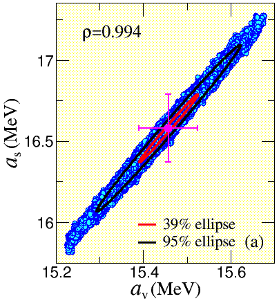
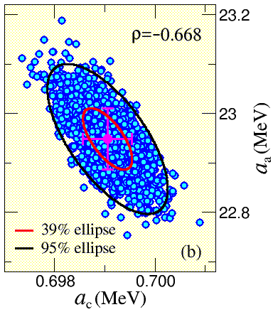
Figure 2: (color online) (a) Correlation plot between the volume and surface terms of the liquid-drop model. The 200,000 points represent the raw data obtained from the Monte-Carlo simulation. Also shown are the 39% (in red) and 95% (in black) confidence ellipses. (b) Same as in (a) but now for the Coulomb and asymmetry terms of the LDM. Here the 1,784 Monte-Carlo points were obtained by performing suitable selection cuts as described in the text.

III.2 Relativistic Energy Density Functional: Calibration and Correlations

In this section we implement the statistical formulation developed earlier to the calibration of a relativistic EDF. In contrast to the liquid-drop model, the high computational demands of the present case preclude us from generating the exact probability distribution. Thus, all our results presented in this section have been obtained in the gaussian approximation.

All the physical observables that will be used in the calibration procedure will be computed using the interaction Lagrangian density of Ref. Mueller and Serot (1996)—properly supplemented by a mixed isoscalar-isovector term Horowitz and Piekarewicz (2001a); Todd-Rutel and Piekarewicz (2005). That is,

$${\mathscr{L}}_{\rm int} = \bar{\psi}\left[g_{\rm s}\phi\!-\!\left(g_{\rm v}V_{\mu}\!+\!\frac{g_{\rho}}{2}{\mbox{\boldmath$\tau$}}\cdot{\bf b}_{\mu}\!+\!\frac{e}{2}(1\!+\!\tau_{3})A_{\mu}\right)\gamma^{\mu}\right]\psi$$ (35)

$$- \frac{\kappa}{3!}(g_{\rm s}\phi)^{3}\!-\!\frac{\lambda}{4!}(g_{\rm s}\phi)^{4}\!+\!\frac{\zeta}{4!}g_{\rm v}^{4}(V_{\mu}V^{\mu})^{2}+\Lambda_{\rm v}\Big{(}g_{\rho}^{2}\,{\bf b}_{\mu}\cdot{\bf b}^{\mu}\Big{)}\Big{(}g_{\rm v}^{2}V_{\nu}V^{\nu}\Big{)}\;.$$

The Lagrangian density includes an isodoublet nucleon field ($\psi$) interacting via the exchange of two isoscalar mesons, a scalar ($\phi$) and a vector ($V^{\mu}$), one isovector meson (${\bf b}^{\mu}$), and the photon ($A^{\mu}$) Serot and Walecka (1986, 1997). The need for large scalar ($g_{\rm s}$) and vector coupling constants ($g_{\rm v}$) is the hallmark of the very successful relativistic mean-field theories Walecka (1974), that account for the saturation of symmetric nuclear matter and the large spin-orbit splitting displayed by finite nuclei. However, to improve the standing of the model the Lagrangian density must be supplemented by scalar and vector self-interactions. In particular, cubic and quartic scalar self-interactions (with coupling constants $\kappa$ and $\lambda$) were first introduced by Boguta and Bodmer in 1977 Boguta and Bodmer (1977) to soften the equation of state (EOS) of symmetric nuclear matter around saturation density. Such a softening is demanded by the measured distribution of isoscalar monopole strength in medium to heavy nuclei, as these are particularly sensitive to the incompressibility coefficient of nuclear matter. Further, the quartic isoscalar-vector self-interaction (with coupling constant $\zeta$) is also responsible for a softening of the EOS of symmetric nuclear matter—but at much higher densities. Indeed, Müller and Serot were able to show that by tuning $\zeta$ one can generate maximum neutron-star masses that may differ by one solar mass, without modifying the behavior of the EOS around saturation density Mueller and Serot (1996). As such, $\zeta$ is fairly insensitive to laboratory observables and must be constrained from astrophysical observations of massive neutron stars Demorest et al. (2010); Antoniadis et al. (2013). Finally, the mixed quartic vector interaction (as described by the parameter $\Lambda_{\rm v}$) was introduced to modify the density dependence of symmetry energy Horowitz and Piekarewicz (2001b), which is traditionally stiff in relativistic models. In particular, tuning this parameter serves to soften the symmetry energy and has a significant impact on the behavior of poorly constrained isovector observables, such as the neutron-skin thickness of heavy nuclei.

The above discussion serves to indicate that the connection between model parameters and physical observables is a complicated one. Indeed, all bulk parameters of nuclear matter—such as the saturation density, binding energy, incompressibility coefficient, symmetry-energy coefficient, and slope of the symmetry energy—are known to involve complicated combinations of the model parameters. Moreover, as argued in the discussion following Eq. (24), the eigenvectors of the matrix of second derivatives also depend on a complicated linear combination of model parameters. In particular, small eigenvalues of the matrix of second derivatives involve linear combinations of coupling constants that are poorly constrained by the objective function. In fact, it was shown in Ref. Fattoyev and Piekarewicz (2011) that one (of the two) linear combination of the isovector parameters $g_{\rho}$ and $\Lambda_{\rm v}$ is very soft and that such linear combination is strongly sensitive to the slope of the symmetry energy. Thus, it seems much more natural to define the objective function $\chi^{2}({\bf p})$ directly in terms of the various bulk parameters of nuclear matter rather than in terms of the coupling constants. This mapping has been shown to be possible in the case of the Skyrme interaction Agrawal et al. (2005); Chen et al. (2010); Kortelainen et al. (2010). As we argue later in Sec. III, the same ideas are used here for the first time in the relativistic case. However, in order to avoid interrupting the flow of the narrative, we only provide here a brief summary of the central points. A detailed account of the transformation between Lagrangian parameters and bulk parameters will be presented in a forthcoming publication Chen and Piekarewicz .

In essence, of the five isoscalar parameters given in Eq. (35), namely, $g_{\rm s}$, $g_{\rm v}$ $\kappa$, $\lambda$, and $\zeta$, the first four can be uniquely determined by specifying four bulk properties of symmetric nuclear matter: (i) the saturation density $\rho_{{}_{\!0}}$, (ii) the binding energy per nucleon $\varepsilon_{{}_{\!0}}$, (iii) the incompressibility coefficient $K$, and (iv) the effective nucleon mass $M^{\ast}$ (all at saturation density). The determination is unique because there is a linear transformation relating the two sets of quantities Glendenning (2000). Left undetermined in the isoscalar sector are then $\zeta$ and the mass of the scalar meson $m_{\rm s}$, which can not be separated from $g_{\rm s}$ in nuclear matter. Note that the mass of the isoscalar-vector (“$\omega$”) meson will be fixed at its experimental value of $m_{\rm v}\!=\!782.5\,$MeV. In the case of the two isovector parameters $g_{\rho}$ and $\Lambda_{\rm v}$, we show in Ref. Chen and Piekarewicz that both of them can be determined from knowledge of the symmetry energy $J$ and its slope $L$ at saturation density. The mass of the isovector (“$\rho$”) meson has been fixed at its experimental value of $m_{\rho}\!=\!763\,$MeV. In this way the objective function $\chi^{2}({\bf p})$ depends on a vector ${\bf p}\!\equiv\!(m_{\rm s},\rho_{{}_{\!0}},\varepsilon_{{}_{\!0}},M^{\ast},K,\zeta,J,L)$ in an 8-dimensional parameter space. Given a point ${\bf p}$ in such a parameter space, the aforementioned transformation is then used to generate the corresponding point ${\bf q}\!=\!(m_{\rm s},g_{\rm s},g_{\rm v},g_{\rho},\kappa,\lambda,\zeta,\Lambda_{\rm v})$ in the space of Lagrangian parameters. Once ${\bf q}$ is determined—and thus all parameters of the Lagrangian—one can calculate all physical observables required to evaluate the objective function. The enormous virtue of this approach is that the objective function is defined in terms of (mostly) physically intuitive parameters rather than in terms of the empirical parameters of the Lagrangian density. Finding out that a large theoretical error is associated to one such physical parameter, say the slope of the symmetry energy $L$, is more informative than discovering a large error in a coupling constant, say $\Lambda_{\rm v}$. Moreover, this choice also significantly improves the efficiency of the calibration procedure as the range of the physical parameters is fairly well constrained.

Once the theoretical model has been defined, one must select the set of observables that will be used in the calibration of the objective function. To this end we have used binding energies and charge radii of the following ten doubly-magic (or semi-magic) nuclei: ¹⁶O, ⁴⁰Ca, ⁴⁸Ca, ⁶⁸Ni, ⁹⁰Zr, ¹⁰⁰Sn, ¹¹⁶Sn, ¹³²Sn, ¹⁴⁴Sm, and ²⁰⁸Pb. Experimental binding energies were obtained from the latest 2012 atomic mass evaluation Wang et al. (2012) and charge radii (except in the cases of ⁶⁸Ni and ¹⁰⁰Sn where they are unavailable) from Ref. Angeli and Marinova (2013). Besides ground-state properties, also included in the calibration are the centroid energies of the isoscalar monopole resonance in ⁹⁰Zr, ¹¹⁶Sn, ¹⁴⁴Sm, and ²⁰⁸Pb. Experimental centroid energies were extracted from Refs. Youngblood et al. (1999); Li et al. (2007); Patel et al. (2013) which include experiments performed at both Texas A&M University (TAMU) and the Research Center for Nuclear Physics (RCNP) in Osaka, Japan. We note that the centroid energy of ²⁰⁸Pb extracted from RCNP ($13.5\pm 0.1$ MeV) is considerably lower than the one extracted from TAMU ($14.18\pm 0.11$ MeV). Implications of this discrepancy on the “softness of Tin” will be addressed in a forthcoming publication. Finally, from the recent observation of 2 solar-mass neutron stars Demorest et al. (2010); Antoniadis et al. (2013), we incorporate in the calibration of the objective function a maximum neutron star mass of $2.1\,M_{\odot}$. The minimization of the objective function and the extraction of the matrix of second derivatives was implemented by employing the Levenberg-Marquardt method—that was found to be both stable and efficient. In analogy to the successful FSUGold parametrization Todd-Rutel and Piekarewicz (2005), the newly calibrated interaction has been named FSUGold 2. A manuscript describing in far greater detail the calibration of FSUGold 2 is forthcoming Chen and Piekarewicz .

Before displaying a few of our results, we summarize some of the central points of the calibration of FSUGold 2. First, we have implemented for the first time in the relativistic approach the transformation from empirical coupling constants to physical parameters. That is, the objective function is defined in terms of bulk parameters of nuclear matter rather than coupling constants. Not only is the implementation more efficient, but the minimization is guided by physical intuition. Second, the calibration of the objective function relies exclusively on measurable quantities—that include ground-state properties of finite nuclei, giant monopole energies, and a maximum neutron-star mass. Finally, other than the recent work of Ref. Erler et al. (2013), we are unaware of any other calibration of an EDF for finite nuclei and neutron stars.

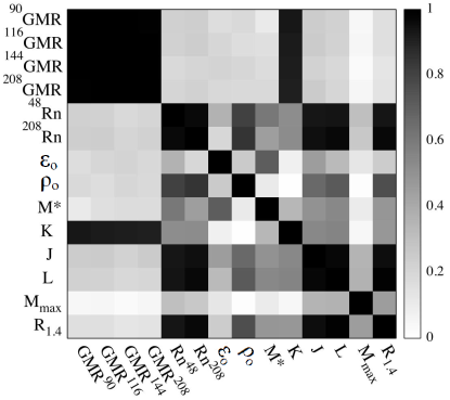
Figure 3: Graphical representation of the correlation coefficients between 14 observables as predicted by the FSUGold 2 effective interaction. The set includes GMR centroid energies for ⁹⁰Zr, ¹¹⁶Sn, ¹⁴⁴Sm, and ²⁰⁸Pb; neutron radii for ⁴⁸Ca and ²⁰⁸Pb; bulk properties of infinite nuclear matter at saturation density ($\rho_{{}_{0}}$, $\varepsilon_{{}_{0}}$, $M^{*}$, $K$, $J$, and $L$); and the maximum neutron-star mass $M_{\rm max}$ and stellar radius $R_{1.4}$ of a 1.4 ${\rm M}_{\odot}$ neutron star.

In Fig. 3 we display in graphical form the correlation coefficients using a set consisting of 14 observables. This set includes GMR energies for ⁹⁰Zr, ¹¹⁶Sn, ¹⁴⁴Sm, and ²⁰⁸Pb; neutron radii for ⁴⁸Ca and ²⁰⁸Pb; bulk properties of infinite nuclear matter at saturation density; and two neutron-star properties: the maximum neutron-star mass $M_{\rm max}$ and the radius of a 1.4 ${\rm M}_{\odot}$ neutron star $R_{1.4}$. With the exception of the centroid energies and $M_{\rm max}$ that were included in the calibration procedure, all the other observables are predictions of the model. Although a thorough analysis of these results will be presented in Ref. Chen and Piekarewicz , we discuss here a few salient features. First and as expected, all GMR energies are strongly correlated to the incompressibility coefficient of symmetric nuclear matter $K$. Second, we have found—as many have before us—a strong correlation between the neutron radius of ²⁰⁸Pb and the slope of the symmetry energy $L$. Our results suggest that such a strong correlation persists between $R_{n}^{208}$ and $R_{1.4}$, even though these quantities differ by 18 orders of magnitude. Finally, the maximum neutron-star mass is weakly correlated to every observable displayed in the figure. This suggests that, whereas laboratory experiments can place significant constraints on fundamental parameters of the nuclear EOS around saturation density, the only meaningful constraint on the high-density component of the EOS of cold neutron-rich matter must come from massive neutron stars.

We finish this section by displaying a correlation plot between the slope of the symmetry energy and the neutron radius of ²⁰⁸Pb. The newly developed relativistic EDF FSUGold 2 predicts: $L\!=\!(112.8\pm 16.1)$ MeV, $R_{n}^{208}\!=\!(5.727\pm 0.019)$ fm, and a robust correlation coefficient of $\rho\!=\!0.966$. This information has been used to produce the 39% and 95% confidence ellipses displayed in Fig. 4. In particular, our results indicate that a 0.3% measurement of $R_{n}^{208}$ would constrain $L$ to about 15%. At present, this 0.3% requirement is beyond the capabilities of the second phase of the Lead Radius Experiment (PREX-II) at the Jefferson Laboratory that aims for a 1% measurement of $R_{n}^{208}$ Paschke et al. (2012). According to our results—by itself—a 1% measurement of $R_{n}^{208}$ will only be able to constrain $L$ to about 50 MeV. However, in combinations with other observables sensitive to the density dependence of the symmetry energy, such as the electric dipole polarizability, one could obtain a significantly more stringent constraint on $L$. Note that with the above value of $R_{n}^{208}$, FSUGold 2 predicts the rather large neutron-skin thickness of $R_{\rm skin}^{208}\!=\!(0.287\pm 0.020)$ fm; for comparison, FSUGold predicts 0.207 fm. This result indicates that as long as the objective function does not incorporate stringent experimental constraints on the isovector sector, relativistic models will continue to predict large neutron skins Lalazissis et al. (1997, 1999). Note that although large, our result is consistent with the pioneering PREX experiment that recently provided, albeit with large error bars, the first model-independent evidence on the existence of a neutron-rich skin in ²⁰⁸Pb Abrahamyan et al. (2012); Horowitz et al. (2012):

$$R_{\rm skin}^{208}\!=\!{0.33}^{+0.16}_{-0.18}\,{\rm fm}.$$ (36)

Moreover, our finding is also consistent with Ref. Fattoyev and Piekarewicz (2013) that recently suggested that well measured physical observables as the ones included in this work, are unable to rule out a thick neutron skin in ²⁰⁸Pb.

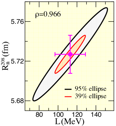
Figure 4: (color online) Correlation plot between the slope of the symmetry energy $L$ and the neutron radius of ²⁰⁸Pb as predicted by the newly developed effective interaction FSUGold 2.

III.3 A Word on Systematic Errors

We close this section with a brief comment on the critical task of estimating systematic errors. Although the FSUGold 2 functional has been accurately calibrated and statistical uncertainties were properly computed, it is not possible to estimate the systematic errors associated with its predictions. Given that FSUGold 2 incorporates its own constraints, limitations, and intrinsic biases, such systematic uncertainties can only be assessed by comparing against the predictions of different models.

To illustrate the role of systematic errors and to continue with our current theme, we display in Fig. 5 predictions for both the slope of the symmetry energy and the neutron-skin thickness of ²⁰⁸Pb for a large number (47) of relativistic and non-relativistic models (this figure has been adapted from Ref. Roca-Maza et al. (2011) with the data kindly provided by X. Roca-Maza). The predictions from FSUGold 2 with its associated theoretical errors are also displayed in the figure. Here $L_{0}\!\equiv\!75.676$ MeV and $R_{0}\!\equiv\!0.212$ fm represent the average values of all 47 predictions. Note that the dispersion in the corresponding average values are $\Delta L\!=\!36.730$ MeV and $\Delta R\!=\!0.055$ fm, respectively. These values are depicted by the (magenta) cross in the middle of the figure. By performing a standard least-squares fit to the predictions of the 47 models, we obtain the following optimal straight line:

$$\left(\frac{R_{\rm skin}^{208}}{R_{0}}\right)=b+m\left(\frac{L}{L_{0}}\right)\;,$$ (37)

with a large correlation coefficient of $\rho\!=\!0.979$, and (dimensionless) slope and intercept given by $m\!=\!(0.524\pm 0.016)$ and $b\!=\!(0.475\pm 0.018)$, respectively. This optimal straight line is displayed by the blue solid line in Fig. 5. Note that the probability distribution of “straight lines” $P(m,b)$ was obtained using maximum-likelihood estimates exactly as before. Indeed, $P(m,b)$ satisfies the same gaussian expression given in Eqs. (26) and (27) for the case of any two generic variables Bevington and Robinson (2003). In the present case, however, the gaussian approximation is exact. Knowledge of the probability distribution $P(b,m)$ not only provides an estimate of the systematics uncertainties in the slope and intercept of the optimal straight line but, in addition, permits to assess the systematic errors in $R_{\rm skin}^{208}$ for any given value of $L$. Doing so results in the $1\sigma$ (in red) and $3\sigma$ (in black) error bands displayed in Fig. 5. That is, the 47 models given in the figure suggest that a “new” model with a value of, for example, $L\!=\!1.5L_{0}$ (as FSUGold 2) will predict a neutron-skin thickness for ²⁰⁸Pb that will have a 68.3% probability of falling within the interval $R_{\rm skin}^{208}\!=\!(1.26\pm 0.01)R_{0}$. Besides being useful in providing an estimate of the systematic errors, plots as the one given in Fig. 5 are useful in quantifying how accurately a measurement (of for example $R_{\rm skin}^{208}$) should be done in order to rule out some theoretical models. Of course, deciding whether a model can be ruled out or ruled in depends critically on the statistical uncertainties predicted by such model, which emphasizes again the importance of providing theoretical uncertainties.

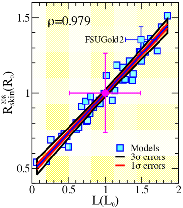
Figure 5: (color online) Predictions for the slope of the symmetry energy and the neutron-skin thickness of ²⁰⁸Pb by a large number (47) of both relativistic and non-relativistic models in units of the corresponding average values $L_{0}\!\equiv\!75.676$ MeV and $R_{0}\!\equiv\!0.212$ fm. The meaning of the optimal straight line and the corresponding error bands are explained in the text. The figure was adapted from Ref. Roca-Maza et al. (2011).

IV Conclusions and Outlook

As aptly captured by the Editors of the Physical Review A Editors (2011), the central goal of this contribution to the focus issue on information and statistics is ‘to discuss the importance of including uncertainty estimates in papers involving theoretical calculations of physical quantities’. Given the impossibility of first-principle calculations of nuclear phenomena using QCD, theoretical nuclear physics must rely on the modeling of such phenomena. In this regard, the most sophisticated theoretical framework is density functional theory. Whereas in principle the empirical constants defining the EDF should be computed from QCD, in practice they are fitted directly to many-body observables. As such, the calibration of the EDF relies on the minimization (or calibration) of a properly defined objective function. Until recently, once the minimum was found the model was validated against observables not included in the fit. More recently, however, the standards have been raised considerably. As properly articulated in Ref. Editors (2011), one now demands predictions to be accompanied by meaningful and reliable theoretical errors.

In this contribution we have framed the formalism in terms of maximum-likelihood estimation. Such an approach is intuitive, transparent, and—at least in principle—straightforward to implement. Once a model has been selected and a set of accurately-measured observables identified, the objective function (e.g., $\chi^{2}$) is defined in terms of the square-differences between these observables and the predictions of the model. The likelihood function—simply obtained from “exponentiation” of the objective function—now acts as an un-normalized probability distribution. In this manner, one could generate, for example via Monte-Carlo methods, the distribution of models in the vast space of parameters. The maximum-likelihood estimate provides the optimal set of parameters, namely, the minimum of the objective function. However, maximum-likelihood estimation goes well beyond providing the optimal model. Indeed, by generating model parameters according to the likelihood function, one can now estimate theoretical errors and correlations among any pair of observables using conventional statistical averaging.

Given its very modest computational demands, we have used the revered liquid-drop model to illustrate the power and elegance of maximum-likelihood estimation (see also Ref. Dobaczewski et al. (2014)). By doing so—not only can we obtain theoretical averages and errors, but in addition—we were able to generate the full probability distribution of the liquid-drop parameters. Moreover, we could assess the degree of correlation among the parameters through highly insightful confidence ellipses. Finally, we relied on this pedagogical model to test the robustness of the gaussian approximation, namely, the approximation in which the deviations from the $\chi^{2}$ minimum are assumed to be quadratic.

For the more realistic case of the optimization of a relativistic EDF, we were limited—because of severe computational demands—to the gaussian approximation. Once the relativistic Lagrangian was defined and physical observables selected (which involve ground-state properties of finite nuclei, giant-monopole energies, and the limiting mass of a neutron star) the minimum of the objective function and its associated matrix of second derivatives were obtained using the Levenberg-Marquardt method. With such information at hand, we were able to compute averages, theoretical errors, and correlation coefficients for various observables. In particular, we concluded that the maximum mass of a neutron star is poorly correlated to a host of laboratory observables—suggesting that the search for massive neutron stars may provide the only meaningful constraint on the EOS of neutron-star matter. A more detailed discussion of these results will be presented in a forthcoming publication Chen and Piekarewicz . We note that the minimization procedure was implemented by using, for the first time in the relativistic approach, a parameter set consisting of physical quantities rather than empirical parameters of the Lagrangian. The transformation from empirical constants to physical quantities provides several important advantages Chen and Piekarewicz .

In summary, we have used central idea from information and statistics—particularly maximum-likelihood estimation—to demonstrate the power of the approach and its critical role in the development of a new paradigm in nuclear theory. The need to quantify theoretical uncertainties is particularly urgent as models that are fitted to experimental data are then used to extrapolate to the extremes of density and isospin asymmetry, such as those encountered in neutron stars. The present focus issue in general—and this contribution in particular—provide detailed derivations and simple examples on how to apply these ideas to the quantification of uncertainties and the analysis of correlations. Besides the obvious benefits, a proper statistical analysis may also improve the control of the systematic errors. Although there are many sources of systematic errors, one that may be readily addressed involves comparison among various accurately-calibrated models. Given that models include intrinsic constraints and limitations, their prediction may vary significantly—even when calibrated to the same set of experimental data. Such systematic uncertainties can only be assessed by comparing different models. However, the predictions from the various models are rarely (if ever) accompanied by their corresponding statistical uncertainties. Hence, it is common practice to simply “throw” all predictions into a plot and then attempt to infer some degree of correlation among the observables of interest. This situation is unsuitable and one should advocate for higher quality control involving, at the very least, theoretical predictions with properly quantified uncertainties. It appears that the contributors to the Physical Review A have adapted well to such higher demands. It is high time for the nuclear-theory community to follow suit.