Influence of primary particle density in the morphology of agglomerates

Abstract

Agglomeration processes occur in many different realms of science such as colloid and aerosol formation or formation of bacterial colonies. We study the influence of primary particle density in agglomerate structure using diffusion-controlled Monte Carlo simulations with realistic space scales through different regimes (DLA and DLCA). The equivalence of Monte Carlo time steps to real time scales is given by Hirsch’s hydrodynamical theory of Brownian motion. Agglomerate behavior at different time stages of the simulations suggests that three indices (fractal exponent, coordination number and eccentricity index) characterize agglomerate geometry. Using these indices, we have found that the initial density of primary particles greatly influences the final structure of the agglomerate as observed in recent experimental works.

PACS numbers

82.70.Rr, 61.43.Hv, 02.70.Uu, 05.10.Ln

Keywords

Brownian motion, Monte Carlo methods, fractal-like aggregates.

I INTRODUCTION

Agglomeration of single particles to generate larger aggregates is an ubiquitous physical phenomenon in nature. Not only the physics and chemistry of colloids and aerosols is governed by agglomeration but also more complex mechanisms occurring in proteins or viruses depend on it Marchetti et al. (2013). Self-propelling active particles such as bacteria, insects, birds or fish may agglomerate to form colonies swarms, flocks or schools Marchetti et al. (2013). Agglomeration of active or passive particles involving Brownian motion is quite common. Inert particles arising from combustion processes may aggregate forming aerosols and soot agglomerates. Soot agglomeration is very important for industry and everyday life. Particulate matter generated during combustion may have undesired effects including corrosion of boiler surfaces caused by particle deposition and chemical activity (fouling), deposition, chemical activity and particle fusion (slagging) Benson et al. (1993), and serious health problems such as pneumoconiosis and lung cancer Hidy (1984).
    Aliphatic and aromatic compounds of hydrocarbons (present in tars) volatilize very quickly (with a characteristic time of about $10^{-4}$ sec. Malte (1979)) and undergo subsequent chemical reactions, leading to the formation of soot particles (which have lost most of their original hydrogen) and polyaromatic hydrocarbons. Primary soot particles are mainly aggregates of thousands of graphitic crystallites whose size is about tens of nanometers Williams et al. (2000). These aggregates tend to stick together immediately after their formation forming “fractal-like” structures. This is the agglomeration process. Additional processes like sintering will affect the shape and properties of the agglomerates at much longer times. Here we want to describe the whole agglomeration process since its early stages and studying the evolution of agglomerate structure. This is important e.g. for understanding vapor condensation on agglomerates in boundary layer flows near the walls of a combustion chamber.
    The literature contains numerous models of agglomeration processes. Many of these works use Langevin equations Mountain et al. (1986); Isella and Drossinos (2010) or kinetic (Smoluchowski) equations written in terms of a collision frequency factor. Many others resort to numerical simulations based on some random-like collision algorithm, e.g. Monte Carlo simulations, based on the solution of the Langevin equation in integral form. A detailed historical review is Meakin (1999). Most importantly, the agglomerates obtained through all these models are fractal-like structures, a consequence that has been validated by many experimental works Samson et al. (1987); Oh and Sorensen (1997); Sorensen (2000); Mulholland et al. (2013). Many works simulate agglomeration starting from a number of particles in a given volume Mountain et al. (1986); Isella and Drossinos (2010); Meakin et al. (1985); Park et al. (2001); Cho et al. (2011). In these works, the calculated fractal exponents of agglomerates range from 1.62 to 1.9, the particle number density is between $10^{14}$ and $10^{15}$ cm^-3 whereas the expected amount of soot in a combustion chamber is in the range of much lower values, $10^{10}\sim 10^{12}$ cm^-3 Samson et al. (1987). In these works, numerical simulations yield fractal exponents of agglomerates between 1.7 and 1.8 which correspond to three-dimensional diffusion-limited colloid aggregation (DLCA). Recently Chakrabarty et al. Chakrabarty (2009) have observed soot fractal aggregates with fractal exponents in the range $1.2\sim 1.5$ from ethene-oxygen premixed flames with $2.3\sim 3.5$ fuel-to-air equivalence ratio. These exponents are noticeably lower than DLCA values (about 1.8 Maricq (2007)).
Although Langevin equations seemingly provide very appropriate ways to tackle agglomeration, their use has been marred by different shortcomings. For instance, Isella and Drossinos Isella and Drossinos (2010) write a Langevin equation for each monomer which is computationally quite costly. Moreover, the equivalent physical time of their simulations is very short because the agglomerates dissolve quickly after being formed. They also use an extremely high particle density, evidently to accelerate the agglomeration process. Mountain et al. Mountain et al. (1986) save computation time by the crude simplification of considering a generic Langevin equation for noninteracting particles.
Here we reproduce the agglomeration process through a Monte Carlo simulation considering that both single particles and the resulting agglomerates undergo Brownian motion. Brownian motion decreases as the particles collide and bond, i.e. agglomerates move more slowly than particles. This speed reduction is due to the increasing frictional resistance of the carrier gas. Different ways of incorporating the frictional resistance of the carrier gas into the simulations include using empirical expressions of diffusive mobility in fractal aggregates coming from laboratory measurements Wang and Sorensen (1999) and assimilating the agglomerate to a porous medium Tandom and Rosner (1995, 1996). A common feature of these methods is that in some step of the process the agglomerate is characterized by a single parameter, which misses somewhat the agglomerate geometry. Instead, we have used the Riseman-Kirkwood theory that incorporates the geometrical configuration of the whole agglomerate in the calculation of the diffusivity (which is obtained at each time step of the simulation)Riseman and Kirkwood (1956). Starting from a uniform spatial distribution, particles and agglomerates move randomly move and interact in a 3D cubic lattice. They evolve from an initial stage of diffusion limited aggregation (DLA), in which clusters grow by aggregating one single particle at a time Halsey (2000), to a later DLCA stage, in which clusters stick to clusters. In order to obtain the equivalency of Monte Carlo times and physical times, the time elapsed during a simulated Brownian jump is calculated using Hinch’s theory of Brownian motion Hinch (1975) which, being local, is consistent with the Riseman-Kirkwood theory (See appendix).
In order to compare our work to previous experimental results Chakrabarty (2009), our simulations have been run up to 6 seconds of equivalent physical time. We have found that the fractal exponents of the agglomerates increase with particle density and we have also studied the effect of the latter on the evolution of the fractal exponents. Another important point in our work is the geometrical characterization of the agglomerates. There are abundant references in the literature to the influence of the prefactor and the fractal exponent in the morphology of the agglomerate. Much more sparse are the references to the coordination number and its influence Isella and Drossinos (2010). In addition to fractal exponent and coordination number, we introduce here the eccentricity index (which has some precedent in the triangle distribution function Hutter (2000)). The geometric mean of the two last indices shows an unexpected regularity for different times, densities and morphologies.
The rest of the paper is organized as follows. In section 2, we describe the simulation algorithm. We describe and discuss our results, validate the model and include a geometrical description of agglomerates in section 3. Section 4 contains our conclusions and the Appendix is devoted to technical matters.

II Simulation details

Initially, $N_{p}=8000$ particles of diameter $d_{p}=50$ nm occupy the nodes of a cubic lattice of side $S_{p}$ Park and Appleton (1973) (see Figure 1). Then the particle number densities are in the range $10^{10}\,\sim\,10^{14}$ cm^-3. Notice that expected soot particle densities inside combustion chambers are in the order of $10^{10}\,\sim\,10^{12}$ cm^-3 Morgan et al. (2007). As we explain in the next section, the selected number of particles allows the particle distribution function to become self-similar, with quasi-steady moments, thereby avoiding boundary effects. Self-similar size distributions have been widely observed in aerosols Friedlander (2000).

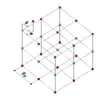
Figure 1: The cubic lattice used in the simulations. Spacing between particles, $S_{p}$ is equal to $\displaystyle{\frac{1}{d_{p}}\left(\frac{1}{n_{p}}\right)^{1/3}}$, where $n_{p}$ is the primary particle number density. Polar and azimuth angles are taken respecting to a coordinate system that moves with the particle or the centroid of the agglomerate.

In the simulations, particles undergo Brownian motion with a fixed length step (which is $h_{p}=2d_{p}$ for single particles) but they move in random directions given by the angles shown in Figure 1. The relation between the simulation time step and real time is such that the root mean square displacement of the particle during a time step is $2d_{p}$. Then Berne and Pecora (1976) (Appendix 5A), Weitz et al. (1989)

$$\sqrt{\langle\Delta x(t)^{2}\rangle}=2d_{p},\,\langle\Delta x(t)^{2}\rangle=2\int_{0}^{t}(s-t)\langle v_{x}(0)v_{x}(s)\rangle ds.$$ (1)

In the simplest case, the velocity autocorrelation is that of an Ornstein-Uhlenbeck process Chandrasekhar (1943); Capasso and Backstein (2012), whereas a more realistic expression is provided by Hinch’s theory of Brownian motion Hinch (1975). Both mean squared displacements are listed in the Appendix. Inserting these expressions in (1) and solving that equation for the time step, we obtain Ornstein-Uhlenbeck and Hinch times. The largest of the two is usually the Hinch time which we select as our time-step. The random polar ($\Phi=\pi\,\delta_{1}$) and azimuthal ($\Theta=2\,\pi\,\delta_{2}$) angles are referred to a coordinate system that moves with each particle. $\delta_{1}$ and $\delta_{2}$ are random numbers uniformly distributed between 0 and 1. This choice avoids unequal chance fluctuations in long sequences of random angles Feller (1968) and it does not require to randomly generate angles out of a uniform spherical distribution as in Wozniak et al. (2012). We have used periodic boundary conditions to preserve the particle density during the simulation, i.e. particles that move out of the domain are re-injected from the opposite boundary.
As agglomeration criterion, we consider that two particles (single or pertaining to an agglomerate) whose centers get closer than $2\,d_{p}$ will agglomerate. We prevent overlapping by calculating if the jump length leading to collision along a random direction is smaller than $2\,d_{p}$. As the agglomerates increase their size, drag forces due to friction with the carrier gas increase too and we expect a reduction in the agglomerate velocity. To take into account this effect, we calculate the translational diffusion coefficient of each agglomerate, anytime a new bond is formed, by means of the Riseman-Kirkwood theory Riseman and Kirkwood (1956):

$$D_{a} = \displaystyle{\frac{D_{p}}{N_{a}}\left(1+\frac{d_{p}}{2\,N_{a}}\sum\limits_{i}\sum\limits_{j}\frac{1}{R_{ij}}\right)}$$

where $D_{p}$ is the particle diffusion coefficient (see Appendix), $D_{a}$ is the agglomerate diffusion coefficient, $N_{a}$ is the number of particles in the agglomerate and $R_{ij}$ is the distance from $i^{th}$ to $j^{th}$ particles in the agglomerate. Notice that as the size of the agglomerate increases, $N_{a}$ increases and then, the diffusion coefficient tends to decrease. The Brownian jump of each agglomerate, $h_{a}$, is given by the following simple rule:

$$h_{a}=h_{p}\frac{D_{a}}{D_{p}}$$

A jump length of $2\,d_{p}$ only occurs for primary particles: the agglomerates jump over smaller distances as they grow. Our algorithm is summarized in the following lines:

1. Set the number of particles and distribute them homogeneously in a cubic lattice.

2. Choose a particle number density which leads to a particle spacing ($S_{p}$) for initial distribution.

3. Fix the size of the primary particle jump ($h_{p}=2d_{p}$) and calculate the physical time ($t_{step}$) corresponding to one simulation time step.

4. Pick a maximum real time for the simulation ($T$)

5. While t $<T$

   1. Generate random angles for each particle/agglomerate in the simulation.

   2. Produce jumps and update positions.

   3. Check distances between external particles and agglomerates and join to the latter all the external particles within a distance $<2d_{p}$ (to prevent overlapping).

   4. Update diffusion coefficients and jump lengths ($h_{a}$).

   5. t = t + $t_{step}$.

6. End

Most Monte Carlo simulations of agglomeration processes use different algorithms for the DLA and DLCA stages Meakin (1999); Meakin et al. (1985); Cho et al. (2011). The particles or clusters that join together and the way they join are determined by a random ad hoc procedure that does not have a correspondence to the actual physical system. Instead, we use a single algorithm that does not distinguish between DLA and DLCA stages. In our algorithm, contacts between particles and clusters and clusters with clusters occur as a result of the Brownian motion of particles and clusters themselves in a real-scale space. We have ignored cluster rotation by simplicity.

III Numerical results and discussion

In our simulations, we have used parameter values corresponding to soot formation inside a combustion chamber as indicated in Table 1. In the Table, $\rho_{\mathrm{p}}$, $d_{p}$, $n_{p}$, $T$, $P_{a}$, $\mu_{a}$, $\rho_{\mathrm{a}}$ and $k_{B}$ are the soot density, the primary particle diameter, the primary particle number density, the air temperature, the air pressure, the air viscosity (calculated using Sutherland relation), the air density (considered as an ideal gas) and the Boltzmann constant, respectively.

$\rho_{p}$	$d_{p}$	$n_{p}$	$T$	$P_{a}$	$\mu_{a}$	$\rho_{a}$	$k_{B}$
(g cm-3)	(nm)	(cm-3)	(K)	(Pa)	(N s m-2)	(kg m-3)	(kg m2 s-2)
$2$	$50$	$10^{10}\,\sim\,10^{14}$	$1900$	$1.01325\times 10^{5}$	$6.20\times 10^{-5}$	0.173	$1.38\times 10^{-23}$

Table 1: Constants and parameters used in the simulation

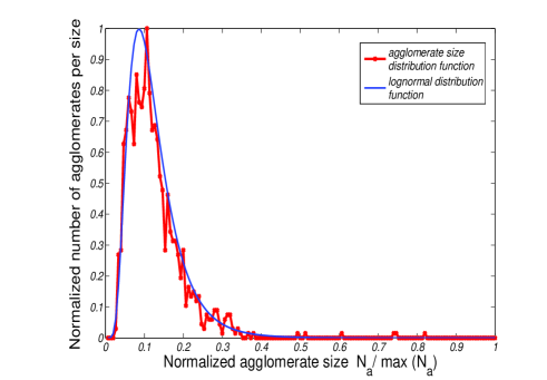
Figure 2: Size distribution function in terms of the scaled size $\xi=i/N(t)$, where $N(t)$ is the number of aggregates at time $t$. The simulation lasts 6 seconds and the initial particle density is $4\times 10^{10}$ cm^-3.

We have computed 100 sets of simulations for a primary particle number density of $4\times 10^{10}$ cm^-3 and 10 sets for other 9 different densities between $10^{10}$ and $10^{14}$ cm^-3 in order to observe the effect of the primary particles density in the resulting structures. 61 samples per simulation were taken to study in detail the time evolution of the system. Simulations for the different densities were run up to 6 seconds of physical equivalent time. We compare the size distribution obtained through our simulations with a lognormal distribution because the latter describes very well atmospheric aerosols, mainly those coming from a single source Hinds (1999). This is shown in Figure 2 for a primary particle number density of $4\times 10^{10}$ cm^-3. For $N_{p}=8000$ particles, the size distribution function becomes self-similar after sufficient time. This implies that there are no boundary effects. To further check this, we have calculated the time evolution of the geometrical as well as the logarithmic moments (from the $2^{nd}$ to the $6^{th}$ moment),

$$\displaystyle{\langle\eta^{k}\rangle} = \displaystyle{\frac{1}{N}\sum_{i}\eta_{i}^{k}n_{i}=\frac{\mu_{k}}{\mu_{1}^{k}}\,N^{k-1}},$$

$$\displaystyle{\langle\left(\ln\eta\right)^{k}\rangle} = \displaystyle{\frac{1}{N}\sum\limits_{i}[\ln\eta_{i}]^{k}\,n_{i}},$$

$$\displaystyle{\mu_{k}} = \sum\limits_{i}i^{k}n_{i},$$

where $\displaystyle{\langle\eta^{k}\rangle}$ is the $k^{th}$ geometric moment of $f(\eta,t)$, $\displaystyle{\langle\left(\ln\eta\right)^{k}\rangle}$ is the $k^{th}$ logarithmic moment of $f(\eta,t)$, $n_{i}(t)$ is the number of agglomerates with $i$ particles at time $t$, $\eta_{i}(t)=\displaystyle{\frac{iN(t)}{\mu_{1}(t)}}$ and $N=N(t)=\mu_{0}(t)$ is the number of agglomerates at time $t$. Assuming that the size distribution function is self-similar, $n_{i}(t)=f(i/N(t))$, and we get

$$\mu_{k}=\int i^{k}f\!\left(\frac{i}{N(t)}\right)\!di=[N(t)]^{k+1}\int\xi^{k}f(\xi)d\xi\Longrightarrow\langle\eta^{k}\rangle=\frac{\int\xi^{k}f(\xi)d\xi}{[\int\xi f(\xi)d\xi]^{k}},$$

so that the $k^{th}$ moment is independent of time. Similarly, the logarithmic moments should be independent of time once the self-similar size distribution is established.

Figure 3 shows the averaged geometric (left) and logarithmic (right) moments for a total number of $8000$ particles. For a physical time of 6 seconds, the lower order geometric and logarithmic moments reach a steady state which indicates that a self-similar size distribution function has been reached. This indicates that we obtain reliable results from simulations with 8000 particles.

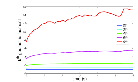
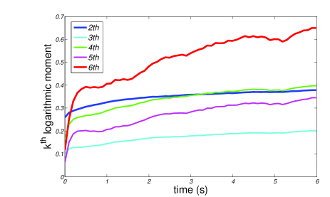
Figure 3: Time evolution of the averaged geometric (left) and logarithmic (right) $\mathit{k^{th}}$ moments, obtained from the simulations.

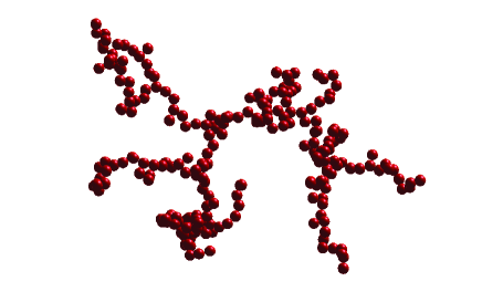
(a)

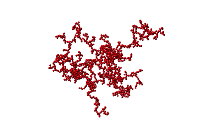
(b)

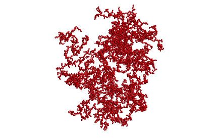
(c)

Figure 4: Different sized agglomerates: (a) with 245 particles, (b) with 1484 particles and (c) with 8000 particles, corresponding to densities $4\times 10^{10}$, $10^{12}$ and $10^{14}$ cm^-3, respectively.

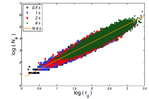
Figure 5: Number of particles per agglomerate versus radius of gyration for a primary particle density of $4\times 10^{10}$ cm^-3 and equivalent physical times of 0.5, 1, 2 and 6 s. Different points correspond to different simulations and we have fit a straight line through the points corresponding to 6 s. Note that there is no indication of transient behavior.

III.1 Fractal exponents of the agglomerates

Figure 4 shows three agglomerates with 245, 1484 and 8000 particles for primary particle number densities of $4\times 10^{10}$, $10^{12}$ and $10^{14}$ cm^-3, respectively. It can be appreciated that very open fractal-like structures appears for low density values, evolving to more compact shapes as the density increases. In an agglomerate, the number of particles $N_{a}$ is related to the radius of gyration $r_{g}$ (mean squared radius) by $N_{a}=k_{a}r_{g}^{E_{f}}$, where $E_{f}$ is the mean fractal exponent $E_{f}$ and $k_{a}$ is a prefactor Friedlander (2000). From the linear fit,

$$\log(N_{a})=\log(k_{a})+E_{f}\,\log(r_{g}),$$

$$r_{g}^{2}=\frac{1}{N_{a}}\sum_{j=1}^{N_{a}}(\mathbf{r}_{j}-\mathbf{\bar{r}})^{2}=\frac{1}{2N_{a}^{2}}\sum_{i,j=1}^{N_{a}}(\mathbf{r}_{i}-\mathbf{r}_{j})^{2}$$

(where $\mathbf{r}_{j}$ is the position of particle $j$ in the agglomerate of size $N_{a}$ and $\mathbf{\bar{r}}$ is the mean position), we can extract the fractal exponent $E_{f}$ that characterizes agglomerates; see Figure 5. Figure 6 shows $E_{f}$ varies with time for different values of the primary particle number density (from $10^{10}$ cm^-3 to $10^{14}$ cm^-3). After a 1 second equivalent physical time, the maximum $E_{f}$ varies between 1.4 and 2.8 for the considered densities, as depicted in Figure 7. The fractal exponent tends to a constant and larger value for larger times (with one exception). Thus the fractal exponent obtained after one second is a lower bound of the asymptotic value of the fractal exponent. In the case of the outlier, with primary particle number density of $10^{14}$ cm^-3, one second is sufficient for bringing to completion the agglomeration process. To attain the asymptotic value of the fractal exponent in that case, we should have used a much larger value of the total number of particles which would have increased considerably the computational cost. The average agglomerates fractal exponents reach values between 1.4 and 2.8 for the range of initial particle densities we use.

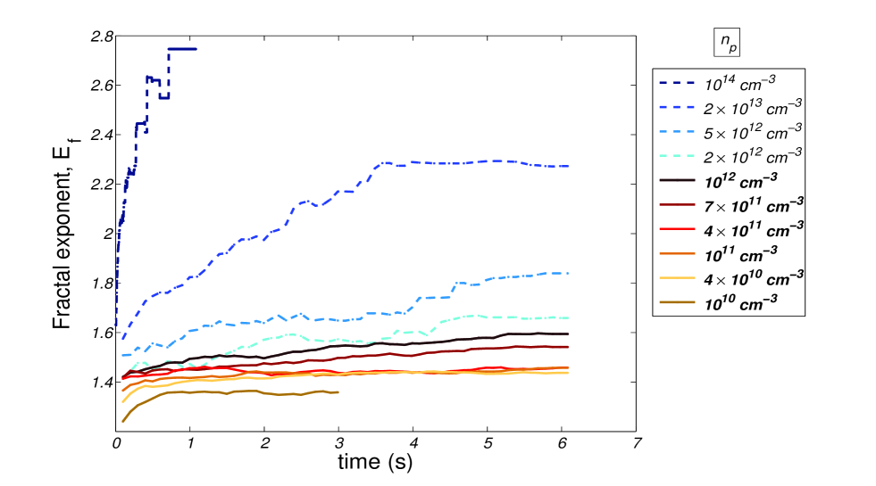
Figure 6: Time evolution of the fractal exponent $E_{f}$ for different primary particle (soot) number densities $n_{p}$. The exponents corresponding to densities seen in combustion processes are depicted as solid lines. The uppermost curve is interrupted because an agglomerate comprising all the particles is formed before 6 seconds.

In the literature, the calculated fractal exponents of agglomerates range from 1.62 to 1.9, for particle number densities between $10^{14}$ and $10^{15}$ cm^-3 Mountain et al. (1986); Isella and Drossinos (2010); Meakin et al. (1985); Park et al. (2001); Cho et al. (2011). These fractal exponents are in the range of 3D DLCA, about 1.8 Maricq (2007). Recently Chakrabarty et al. have observed soot fractal aggregates with much lower fractal exponents in the range $1.2\sim 1.5$ from ethene-oxygen premixed flames with $2.3\sim 3.5$ fuel-to-air equivalence ratio. While these fractal exponents are lower than those found in the literature Mountain et al. (1986); Isella and Drossinos (2010); Meakin et al. (1985); Park et al. (2001); Cho et al. (2011), the initial number density in the experiments is in the range $10^{10}\sim 10^{12}$ cm^-3, which is also lower than the $n_{p}$ values used in the numerical works. The fractal exponents observed in experiments are like those found in our simulations for the same number density range. Note that the fractal exponent rises more abruptly for $n_{p}$ above $10^{12}$ cm^-3 to within the DLCA range found in Mountain et al. (1986); Isella and Drossinos (2010); Meakin et al. (1985); Park et al. (2001); Cho et al. (2011).

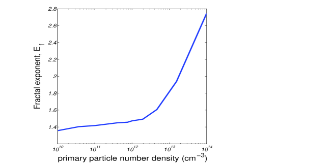
Figure 7: Fractal exponent $E_{f}$ versus primary particle number density $n_{p}$ after 1 second. The steeper part, at the right, is indicating that bigger clusters are formed more rapidly due to the higher densities of primary particles ($>2\times 10^{12}$ cm^-3).

III.2 Geometrical characterization of the agglomerates

In addition to the fractal exponent, we may characterize agglomerates by other indices of geometrical nature. In an agglomerate, the relative number of particles $n_{g}^{j}$ surrounding a given one $j$ (at a distance not larger than $2d_{p}$) gives an idea of the compactness of the latter, and we call it coordination index,

$$i_{c}^{j}=\displaystyle{\frac{n_{g}^{j}}{12}}\in[0,1],\qquad\text{coordination index of $j^{th}$ particle.}$$

$i_{c}^{j}=0$ corresponds to an isolated particle and $i_{c}^{j}=1$ gives close packing of the particle. The coordination number defined as in Isella and Drossinos (2010) is twelve times our coordination index.

We have also defined the eccentricity index as follows:

$$i_{e}^{j} = \displaystyle{\frac{|\mathbf{r}_{CM}-\mathbf{r}_{j}|}{r_{e}}},\qquad\text{eccentricity index of $j^{th}$ particle}$$

where $\mathbf{r}_{CM}$ is the position of the center of mass of the system formed by the $j^{th}$ particle at $\mathbf{r}_{j}$ and its surrounding neighbors (at distances no larger than $2d_{p}$), and $r_{e}$ is the enveloping radius that corresponds to the maximum distance between the center of mass of the system and the center of the neighbors surrounding the $j^{th}$ particle. This eccentricity index measures the way the particles connect in an agglomerate. A particle with $i_{e}=0$ is surrounded in a spherically symmetric way, whereas a particle with $i_{e}=1$ has the most asymmetric distribution of its surrounding particles.

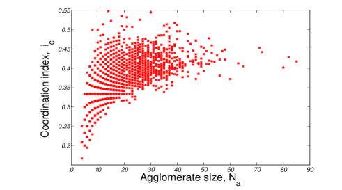
Figure 8: Coordination index of aggregates in terms of its size for different simulations and a primary particle number density $n_{p}=4\times 10^{10}$ cm^-3.

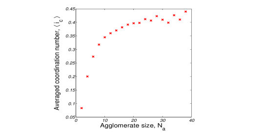
(a)

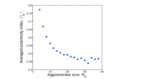
(b)

Figure 9: (a) Variation of the average coordination index $\langle i_{c}\rangle$ with agglomerate size, $N_{a}$. (b)Variation of the mean eccentricity index $\langle i_{e}\rangle$ with agglomerates size $N_{a}$. Primary particle (soot) number density in both plots is $10^{10}$ cm^-3 for an equivalent physical of 1 sec.

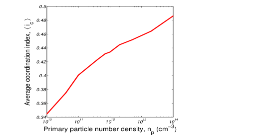
Figure 10: Average coordination index $i_{c}$ of all aggregate sizes versus primary particle number density $n_{p}$ after 1 second equivalent physical time.

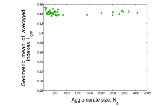
(a)

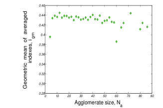
(b)

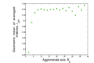
(c)

Figure 11: Geometric mean of the average coordination and eccentricity indices vs agglomerate size after 1 second for three different values of $n_{p}$: (a) $4\times 10^{10}$ cm^-3, (b) $10^{12}$ cm^-3 and (c) $10^{14}$ cm^-3.

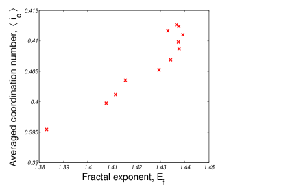
Figure 12: Evolution of the fractal exponent and the coordination index, for a primary particle density of $4\times 10^{10}$ cm^-3, considering sizes $>15$. Each point represents values at a given time and, as time increases, these points tend to accumulate in the upper part of the figure.

The coordination index of an agglomerate is calculated as the mean value of the coordination indices of all the particles comprising it. The same applies for the eccentricity index. These coordination and eccentricity indices depend on the agglomerate size $i$, the realisation of the Brownian motion $\omega$ and the particle number density $n_{p}$, $i_{c,e}(i,n_{p},\omega)$. For a given value of primary particle number density, the coordination indices versus size for different realisations of noise (corresponding to different simulations) are depicted in Figure 8. The expected values of the indices (over all simulations) are the average indices $\langle i_{c}\rangle(i,n_{p})$ and $\langle i_{e}\rangle(i,n_{p})$. Figures 9 (a) and (b) show the average coordination and eccentricity indices for $n_{p}=10^{10}$ cm^-3. Note that $\langle i_{c}\rangle$ increases with agglomerate size, whereas $\langle i_{e}\rangle$ decreases. As the agglomerate size increases, the agglomerates change from being stringy structures with low $\langle i_{c}\rangle$ and large $\langle i_{e}\rangle$ to becoming more compact, with both indices about 0.45; see Figure 4. Figure 10 shows the variation of the average coordination index of all the agglomerate sizes (calculated after a 1 second equivalent physical time) with the primary particle number density. Similarly to the fractal exponent behavior in Fig. 7, this index increases with the density $n_{p}$.

The coordination and eccentricity indices and their geometric mean have the following properties:

• The plot of $i_{c}(i,n_{p},\omega)$ as a function of $i$ in Figure 8, for $n_{p}=4\times 10^{10}$ cm^-3 and different realisations, has a very organized pattern for low $n_{p}$ but does not present a recognisable structure for high $n_{p}$ (e.g., for $10^{14}$ cm^-3).

• $i_{c}$ and $i_{e}$ exhibits an asymptotic behavior for large $N_{a}$ as Figure 9 shows (see also Weber and Friedlander (1997); Isella and Drossinos (2010)). The evolution to constant values of these geometric parameters and of the fractal exponent for large times is a sign that the internal structure of the agglomerate tends to become self-similar. The aggregates grow with time and, as they become larger, they become closer to self-similar and some connectivity pattern is repeated.

• The average indices $\langle i_{c}\rangle$ and $\langle i_{e}\rangle$ probe the local structure of aggregates and they seem to be related for large aggregate size. Their geometric mean, $i_{gm}=\sqrt{\langle i_{c}\rangle\,\langle i_{e}\rangle}$, becomes almost constant for large $N_{a}$, as shown in Figure 11 for three different densities. As the aggregates size $N_{a}$ grows, the increasing coordination index and the decreasing eccentricity index seem to compensate. Assuming an ad hoc very dense particle packing representing an upper limit for $i_{c}$, we have created a sequence of configurations and obtained the geometric mean $i_{gm}$ which is bounded between 0.4 and 0.5.

• The cluster distribution evolves to become self-similar and, at the same time, the fractal exponent and the coordination index evolve to constant values as shown in the highest part of Figure 12, where points accumulate. Both the fractal exponent (Fig. 7) and the average coordination index (Fig. 10) of all the agglomerate sizes increase with the primary number density $n_{p}$. This seems reasonable as they both probe the self-similar structure of the clusters and are therefore related.

IV Concluding remarks

We have simulated the agglomeration of single particles for different initial number densities by a Monte Carlo method. The range of initial number densities covers the values expected for soot particles in combustion processes and also higher values used by other authors in their simulations Mountain et al. (1986); Isella and Drossinos (2010). Initially, 8000 particles occupy a cubic domain with periodic boundary conditions (to preserve particle density). This size produces a self-similar log-normal size distribution function after a short time with quasi-steady moments. After an equivalent physical time of one second, a self-similar size distribution is reached. The fractal exponent increases with primary particle number density, first slightly and, beyond $n_{p}=10^{12}$ cm^-3, more abruptly. Below that density, the fractal exponent is no larger than 1.5 and it remains so no matter the duration of the process. For such low densities, particle spacing is much larger than particle size. Then the agglomerates are elongated and tree-like even at the beginning of the aggregation process. This is particularly true for small agglomerates as confirmed by the small value of the coordination index and the larger eccentricity index. These indices give a more complete description of the agglomeration process than the fractal exponent and its prefactor Heinson et al. (2010) alone. In fact, these indices provide information about the local connectivity and mass distribution inside the agglomerate. Their behavior in terms of agglomerate size is opposite, the average coordination (eccentricity) index increases (decreases) with agglomerate size so that the geometric mean of both indices is roughly constant with agglomerate size.

The main achievements of our work can be recapitulated as follows:

• The fractal exponent is not a fixed value determined by the kind of aggregation process (DLA or DLCA) that has taken place. Instead the fractal exponent is closely related to the density of primary particles that will agglomerate. We base this assertion on Monte Carlo simulation results carried out in real physical space.

• The aggregates are characterized by the fractal exponent and by two other geometric parameters, the coordination and eccentricity indices. The behaviors of these indices reinforce the conclusion that aggregates become self-similar for large times if their size is sufficient. The geometric mean of the coordination and eccentricity indices is almost the same for different primary densities (and therefore for different fractal exponents) which suggest that these indices are related once self-similarity has set in.

Although our simulations refer to particle agglomeration during combustion, the simulation algorithm is applicable to many other agglomeration processes. In particular, we may also generalise the algorithm to include thermophoretic forces over the agglomerates during agglomeration. We are currently working in this direction.

Appendix: Physical time equivalence

To establish the simulation time step according to (1), we need the time-dependent mean squared displacement of a particle, $\langle\Delta x^{2}\rangle$. For the Ornstein-Uhlenbeck velocity autocorrelation, (1) is

$$\langle\Delta x^{2}\rangle = 2D_{p}\displaystyle{\left\{t+\varTheta\left[\exp\left(-\frac{t}{\varTheta}\right)-1\right]\right\}}$$

$$\varTheta = \displaystyle{\frac{m}{\zeta}}\,,\quad\quad\quad\text{particle relaxation time}$$

$$D_{p} = \displaystyle{\frac{k_{B}T}{\zeta}}\,,\quad\quad\text{particle diffusion coefficient}$$

$$\zeta = \displaystyle{\frac{3\,\pi\,\mu_{a}\,d_{p}}{C}}\,,\quad\quad\text{particle friction coefficient}$$

$$C = 1+\displaystyle{\frac{2\,l_{a}}{d_{p}}\left[1.257+0.4\exp\left(-\frac{0.55\,d_{p}}{l_{a}}\right)\right]}\,,$$

$$l_{a} = \displaystyle{\frac{1}{\sqrt{2}\,\pi\,d_{a}^{2}\,n_{a}}}\,,\quad\text{mean free path of air molecules,}$$

where $C$ is the slip correction factor, $m$ is the particle mass, $T$ is the fluid (air) temperature, $d_{a}$ is the fluid (air) mean molecular diameter, $n_{a}$ is the fluid (air) number density and $\mu_{a}$ is the fluid (air) viscosity.

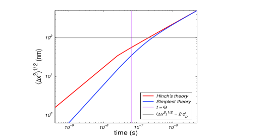
Figure 13: Mean-square displacement as a function of time according to Hinch’s and the simplest theory of Brownian motion. Time step corresponding to the adopted jump length of $2\,d_{p}$ ($10^{2}$) is greater than the particle relaxation time ($\Theta$), as indicated.

Hinch’s theory of Brownian motion takes the hydrodynamic interactions between particles and fluid into account, and it produces the following mean squared displacement Weitz et al. (1989):

$$\langle\Delta x^{2}\rangle = 2D_{p}\displaystyle{\left\{t-2\sqrt{\frac{\tau\,t}{\pi}}+\frac{2\tau}{9}\left(1-\frac{\rho_{p}}{\rho_{a}}\right)+\frac{3}{\sqrt{\tau(5-8\rho_{p}/\rho_{a})}}\left[\frac{1}{a_{+}^{3}}\mathrm{e}^{a_{+}^{2}t}\mathrm{erfc}(a_{+}\sqrt{t})-\frac{1}{a_{-}^{3}}\mathrm{e}^{a_{-}^{2}t}\mathrm{erfc}(a_{-}\sqrt{t})\right]\right\}}$$

$$a_{\pm} = \displaystyle{\frac{3}{2}\left[\frac{3\pm\sqrt{5-8\rho_{p}/\rho_{a}}}{\sqrt{\tau}(1+2\rho_{p}/\rho_{a})}\right]}$$

$$\tau = \displaystyle{\frac{d_{p}^{2}\,\rho_{a}}{4\,\mu_{a}}},\qquad\text{time for diffusion of vorticity across a particle radius}$$

where $\rho_{p}$ is the particle mass density, and $\rho_{a}$ is the fluid (air) mass density. The slip correction factor makes these expressions to be valid for both the continuum and the free molecular regimes. The time corresponding to a jump length of $2\,d_{p}$, according with the Hinch’s theory is $2\times 10^{-7}$ sec. approximately, which is larger than the particle relaxation time as it can be seen in Figure 13.

References

- Marchetti et al. (2013) M. C. Marchetti, J. F. Joanny, T. B. Liverpool, J. Prost, M. Rao, and R. A. Simha, R. Modern Phys. 85, 1143 (2013).
- Benson et al. (1993) S. A. Benson, L. J. Michael, and J. N. Harb, Fundamentals of Coal Combustion (Elsevier (Edited by L. D. Smoot), 1993).
- Hidy (1984) G. M. Hidy, Aerosols: an industrial and environmental science (Academic Press, 1984).
- Malte (1979) P. C. Malte, Pulverized-Coal Combustion and Gasification (Plenum Press (Edited by L. D. Smoot and D. T. Pratt), 1979).
- Williams et al. (2000) A. Williams, M. Pourkashanian, and J. M. Jones, Combustion and Gasification of Coal (Taylor & Francis, 2000).
- Mountain et al. (1986) R. D. Mountain, G. W. Mulholland, and H. Baum, J. Colloid Interface Sci. 114, 67 (1986).
- Isella and Drossinos (2010) L. Isella and Y. Drossinos, Phys. Rev. E 82, 011404 (2010).
- Meakin (1999) P. Meakin, J. Sol-Gel Sci.& Tech. 15, 97 (1999).
- Samson et al. (1987) R. J. Samson, G. W. Mulholland, and J. W. Gentry, Langmuir 3, 272 (1987).
- Oh and Sorensen (1997) C. Oh and C. M. Sorensen, J. Aerosol Sci. 28, 937 (1997).
- Sorensen (2000) C. M. Sorensen, J. Aerosol Sci. 31, S952 (2000).
- Mulholland et al. (2013) N. Mulholland, M. Kraft, M. Balthasar, D. Wong, M. Frenklach, and P. Mitchell, Aerosol Sci. & Tech. 47, 520 (2013).
- Meakin et al. (1985) P. Meakin, Z. Y. Chen, and J. M. Deutsch, J. Chem. Phys. 82, 3786 (1985).
- Park et al. (2001) H. Park, S. Kim, and H. Chang, J. Aerosol Sci. 32, 1369 (2001).
- Cho et al. (2011) K. Cho, K. S. Chung, and P. Biswas, Aerosol Sci. & Techn. 45, 740 (2011).
- Chakrabarty (2009) C. M. Chakrabarty, Phys. Rev. Lett. 102, 235504 (2009).
- Maricq (2007) M. M. Maricq, J. Aerosol Sci. 38, 141 (2007).
- Wang and Sorensen (1999) G. M. Wang and C. M. Sorensen, Phys. Rev. E 60, 3036 (1999).
- Tandom and Rosner (1995) P. Tandom and D. E. Rosner, Ind. Eng. Chem. Res. 34, 3265 (1995).
- Tandom and Rosner (1996) P. Tandom and D. E. Rosner, Chem. Eng. Communic. 151, 147 (1996).
- Riseman and Kirkwood (1956) J. Riseman and J. G. Kirkwood, Rheology (Academic Press (Edited by F. R. Eirich), 1956).
- Halsey (2000) T. C. Halsey, Phys. Today 53, 36 (2000).
- Hinch (1975) E. J. Hinch, J. Fluid Mech. 72, 499 (1975).
- Hutter (2000) M. Hutter, J. Colloid Interface Sci. 231, 337 (2000).
- Park and Appleton (1973) C. Park and J. P. Appleton, Comb. & Flame 20, 369 (1973).
- Morgan et al. (2007) G. W. Morgan, L. Zhou, M. R. Zachariah, W. R. Heinson, A. Chakrabarti, and C. Sorensen, Proc. Comb. Inst. 31, 693 (2007).
- Friedlander (2000) S. K. Friedlander, Smoke, dust and haze. Fundamentals of Aerosol Dynamics, 2nd edition (Oxford, 2000).
- Berne and Pecora (1976) B. J. Berne and R. Pecora, Dynamic light scattering (Wiley, N.Y., 1976).
- Weitz et al. (1989) D. A. Weitz, D. J. Pine, P. N. Pusey, and R. J. A. Tough, Phys. Rev. Lett. 63, 1747 (1989).
- Chandrasekhar (1943) M. Chandrasekhar, Review Modern Phys. 15, 1 (1943).
- Capasso and Backstein (2012) V. Capasso and D. Backstein, An Introduction to Continuous-time Stochastic Processes, 2nd ed. (Birkhaüser, 2012).
- Feller (1968) W. Feller, An Introduction to Probability Theory and its Applications, volume I, 3rd ed. (John Wiley & Sons, 1968).
- Wozniak et al. (2012) M. Wozniak, F. R. A. Onofri, S. Barbosa, J. Yon, and J. Mroczka, J. Aerosol Sci. 47, 12 (2012).
- Hinds (1999) W. C. Hinds, Aerosol Technology: Properties, Behavior and Measurements of Airborne Particles, 2nd ed. (John Wiley & Sons, 1999).
- Weber and Friedlander (1997) A. P. Weber and S. K. Friedlander, J. Aerosol Sci. 28, Suppl. 1, S765 (1997).
- Heinson et al. (2010) W. R. Heinson, C. M. Sorensen, and A. Chakrabarti, Aerosol Sci. & Tech. 44, i (2010).