A Centralized Mechanism to Make Predictions
Based on Data From Multiple WSNs

Abstract

In this work, we present a method that exploits a scenario with inter-Wireless Sensor Networks (WSNs) information exchange by making predictions and adapting the workload of a WSN according to their outcomes. We show the feasibility of an approach that intelligently utilizes information produced by other WSNs that may or not belong to the same administrative domain. To illustrate how the predictions using data from external WSNs can be utilized, a specific use-case is considered, where the operation of a WSN measuring relative humidity is optimized using the data obtained from a WSN measuring temperature. Based on a dedicated performance score, the simulation results show that this new approach can find the optimal operating point associated to the trade-off between energy consumption and quality of measurements. Moreover, we outline the additional challenges that need to be overcome, and draw conclusions to guide the future work in this field.

1 Introduction

Nowadays, forests, cities and houses, among others, are monitored by multiple Wireless Sensor Networks (WSNs) that may belong to different organizations, both public and private, as well as to individual citizens. In addition, there is a high heterogeneity regarding the technologies, protocols and standards used in WSNs. In this situation, each WSN usually operates completely independent of other WSNs, even if they are covering the same physical area, and is thus not able to take any advantage of the presence of those other WSNs to enrich its collected data nor to optimize its operation.

However, WSN performance can be improved by combining data generated from different sensors, belonging to the same node, other nodes from the same network or from other WSNs. This data sharing allows each WSN to build a deeper knowledge about its surroundings, may reduce the probability of getting wrong values and taking wrong decisions, and encompasses wider areas and different perspectives of the same environment.

In an era of high availability of data from the cloud, we are interested in using data from other WSNs to reduce the energy consumption and improve the quality of the measurements done by a target WSN. The external information will be used to make predictions and change the operation of the nodes and save energy when the environmental conditions do not indicate that big changes will happen in the near future. For example, relative humidity and temperature values usually have a high correlation, and the former may have a higher variation if the latter is changing.

This paper lists some of the existing alternatives for collaboration and prediction in WSNs and develops further the inter-WSNs information exchange concept introduced in [1] and in [2]. The main idea behind the inter-WSN information exchange is that the data gathered by other WSNs can be exchanged via their sinks and used to improve the operation of the target one, and vice versa. Our main contribution is a mechanism that uses the data from collaborating WSNs to make predictions. In order to validate our idea, we show how the WSNs evolve using this kind of collaboration, define a way to scale the quality of the measurements and the WSNs’ performance, and finally present some simulation results from a chosen scenario consisting of two WSNs, one for monitoring the relative humidity and another for the temperature. Based on the presented results, we show how energy-efficient and accurate it can be.

The paper is organized in the following sections: In Section 2, we describe related works about collaboration between WSNs, the use of data from external sensors and predictions in WSN environments; the details of our proposed mechanism are explained in Section 3; the use case considered for the tests is detailed in Section 4; the simulation results and the evaluation of the approach are explained in Section 5 and; at the end, our conclusions and ideas for future work are shown in Section 6.

2 Related Work

A system that combines the action of individual components may produce better results than the individual components acting separately. Supported by this premisse, several collaboration mechanisms in WSNs have been developed. Most of the approaches explore the collaboration between sensor nodes of the same WSN. In contrast to them, we extend the concept of collaboration to an upper layer and build the information exchange between different WSNs, without losing any other possible collaboration from the other levels.

An inter-domain routing protocol is described in [3], where it is shown that the gateways may share information about their nodes and take advantage of being physically close to each other. This information can be used to transmit packets through nodes of the other WSNs and can be done either to share the information or for routing purposes. Even though the idea of our work is to create a link between nodes from different WSNs, it is neither meant to share resources nor information between wireless sensor nodes, but the knowledge that the network is able to produce based on collected data.

In [4], the authors describe a scenario where a system is responsible for building a richer knowledge about the environment by making use of the information produced by other WSNs. In their example, wireless sensor nodes combine sensory information with their localization and help other systems to localize and track objects from a distance. The goal of the described approach is to enable a robot to use the data retrieved by a WSN that detects the presence of objects inside the monitored area. After receiving the information from the WSN, the robot interprets the position of the object and moves itself to its location in order to get more details about the real situation. Their approach is different from ours mainly because it uses a non-generic solution that is highly coupled to the presented scenario without a WSN as the beneficiary of the collected information, besides not making any prediction with the information received from the others.

Besides the works that encourage the collaboration among WSNs, some authors applied predictions in order to reduce the energy consumption in the WSNs and extend their lifetime. In [5], the authors developed an algorithm for WSN applications that require a continuous delivery of sensor measurements, such as temperature and traffic monitoring. In order to build sets of nodes that provide trustful measurements, it considers that a sensor measurement is predictable if the predicted value (on average) differs on less than a (user) defined threshold when using other nodes’ measurements. After defining which sensors can be predicted by which other, the base station must find a set of subsets of active nodes such that a different prediction subset is used at each time, and such that all sensors are queried at least once during a cycle. After building this set, the base station must activate a subset of nodes at a time. In other words, only the sensor nodes from the active subset are activated during a time interval and all the others have their radios and sensors turned off in order to save energy and extend the WSN lifetime. Simulations using real data show that such approach can successfully achieve its goals depending on the user requirements and on the quality of the data. Similarly, our mechanism also assumes the task of selecting which sensors are going to be active in the next time interval. However, our mechanism is able to react to environmental changes, while their work is less dynamic. That is, once the sets of sensors are defined, they will be interleaved independently of changes that may happen around the WSN. We highlight that it may be possible to improve our mechanism by adopting their techniques to build the groups of sensors in a way that there is no reduction in the quality of the measurements and the energy savings are maximized.

The solution presented in [6] (called BBQ) is a centralized mechanism used to query data based on sensor models. It assumes that the costs of retrieving data from many nodes can be extremely high and that sensors in close proximity are likely to have correlated readings, which may mean that most of the data provides little benefit in the quality of the answers given to the user. In order to save energy, the BBQ incorporates statistical models of real-world processes into the query processing architecture and acquires data from the sensors only when the model itself is not sufficiently rich to answer the query with acceptable confidence. To achieve such a goal, the BBQ approximates the probability density function of the measurements to multivariate Gaussian distributions and, given the correlation between the known measurement(s) and the unknown one(s), it calculates their expected value associated to a confidence interval. If the confidence level is greater or equal than a chosen threshold, it assumes that such value satisfies the system requirements. Otherwise, it calculates the energy consumed to retrieve new measurements considering the costs to activate the corresponding sensor and, finally, builds a query that will require the lowest energy consumption for the WSN and will give at least the minimum level of confidence set by the user. Similarly to our mechanism, it exploits the correlation between different types of data that the sensor nodes may be able to measure, for example, their own voltage and the local temperature. The difference from our work is that they do not provide a method to measure the quality of the measurements and the performance of the system.

3 Proposed Mechanism

Our system architecture is ready to use information from external WSNs, as described in [1] and [7]. To achieve the goal of optimizing the performance of the WSNs, they must be interconnected through their respective Enhanced Gateways (EGs). We explain the details of the mechanism in the following.

3.1 Centralized Decisions

Periodically, the data retrieved by the nodes are transmitted to the sink. After receiving all the measurements, the sink computes the received values before reporting them to the EG${}_{\text{}}$, which may forward them to external WSNs. In parallel, the EG${}_{\text{}}$ may also receive information from external WSNs and, up to this point, all the data are collected and stored for further analysis. In intervals, the EG${}_{\text{}}$ uses the collected data to predict if there will be changes in the near future. Figure 1 describes the possible states of a WSN.

The predictions done by the EG${}_{\text{}}$ can have two different outcomes: positive, when changes in the environment are expected; and negative, otherwise. If an EG${}_{\text{}}$ receives information from internal and external sources, each prediction may be based on a different data type and independent for each metric. In such cases, they can be combined in order to produce only one outcome. The outcomes can be compared with the real observations in order to verify the performance of the predictions. The feedback can be incorporated by the EG${}_{\text{s}}$ in order to improve their future decisions.

(a) State 1: Nodes report measured values to the sink.

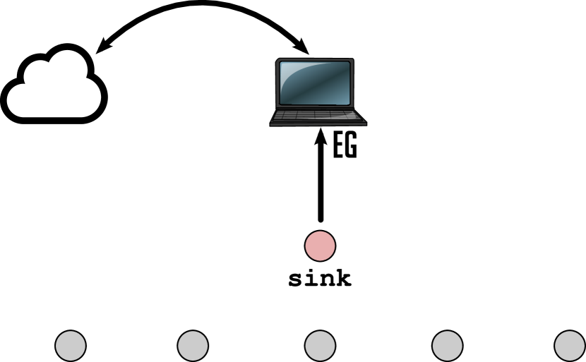
(b) State 2: The sink transmits to the EG the sampled data, which can be forwarded to other EGs at the same time as they transmit to this WSN.

(c) State 3: EG computes a new plan for the nodes and transmits the new configuration to its sink.

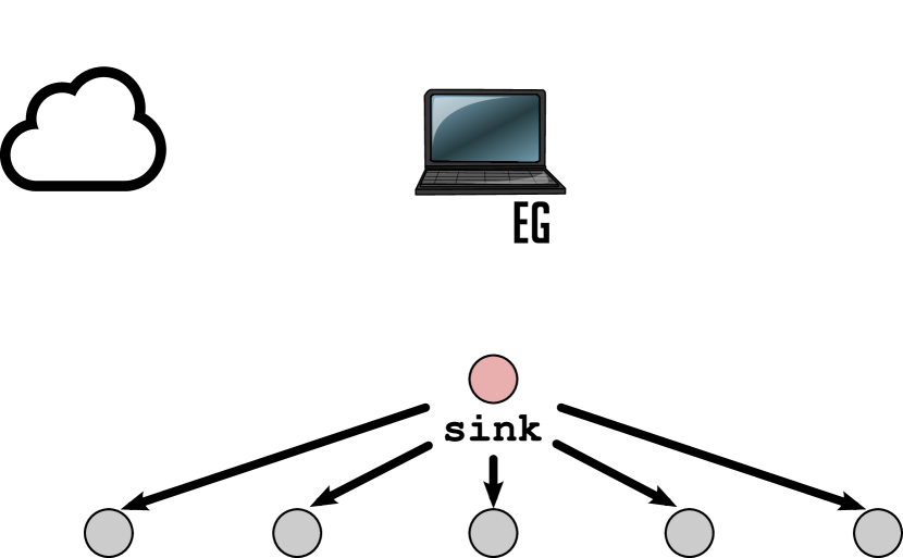
(d) State 4: The sink updates the nodes’ configuration.

Figure 1: Different states of a WSNs using inter-WSN information exchange

3.2 Applications

Based on the outcome of its prediction, a EG${}_{\text{}}$ selects the new strategy that the WSN must follow and will be applied by the sink. At the end, the sink transmits to its nodes a new configuration that they must follow in the next time interval, which may be an instruction to (de)activate themselves or to change the sensing intervals:

3.2.1 Adaptive sensor nodes selection

This application reduces the energy consumption of the network by deactivating some nodes during a certain period of time. In other words, when a node is deactivated, it does not make any measurement, but it may forward messages exchanged by their neighbors. We recall that the sets of active nodes can follow the guidelines described in [5], so the energy savings can be maximized without compromising the quality of the measurements.

3.2.2 Adaptive sampling

Differently from the other application, this solution does not change the number of active nodes. However, when the EG${}_{\text{}}$ has a positive outcome and changes are expected in the environment, the nodes should reduce the time between two consecutive measurement transmissions, consuming more energy and producing more information about the environment. Otherwise, the energy can be saved, because it is not expected big changes in the environment.

3.3 Quality of Measurements (QoM)

As explained before, one of the goals of this mechanism is to reduce the energy consumed in a WSN without reducing the QoM (i.e., a parameter that evaluates if the gathered information from the environment during a certain period is enough to accurately represent it). However, the level of the QoM depends on the type of information reported by the nodes.

We consider monitoring WSNs that make continuous transmissions to the sink and tolerate a small number of packet losses as well as delays between consecutive transmissions, but do not allow the reduction of the covered area because it might miss changes occurring in certain subareas. Therefore, we scaled the QoM as shown in Table 1. There, each interval with a positive outcome should be covered by more reports, increasing the level of knowledge about the environment. Although a high number of measurements always represents a good QoM, the intervals with a negative observation can be covered by less reports without compromising the quality, thereby saving energy. Periods with a negative observation that are wrongly predicted mean that the system expected to have a positive observation in them, produced more measurements and, thus, wasted energy. Differently from the states that a positive is observed and the WSN produced a low number of measurements, those periods still have a good QoM, but the energy consumption might have been reduced and the WSN lifetime increased.

		Prediction outcome
		positive	negative
Actual observation	positive	GOOD	BAD
	negative	GOOD	GOOD

Table 1: Definition of QoM.

Based on this, the accuracy was defined as the percentage of intervals in a day in which the system was operating in a highlighted state. Moreover, the accuracy of positives is the percentage of intervals with positives covered by a high number of measurements.

Regarding the system operation, during intervals in which variations are predicted and the predictions have positive outcomes, the EG${}_{\text{}}$ updates the operation of its WSN in order to collect more information. Each update on its operation affects either the number of active nodes or the time interval between two measurements done by the sensors. As a consequence of this, the number of measurements, the number of transmissions and the energy consumption have higher values during these periods of time, while the opposite effect occurs when no variation is predicted.

3.4 Performance score

In order to evaluate how efficient the use of external information can be, we developed a way to compare the approaches. For a given scenario, we calculate the lowest energy consumption that the WSN may have ($E_{\text{min}}$), which can be done by always setting the plan that produces less measurements during a day. On the other hand, we measure how much energy is consumed by the WSN when it produces the maximum number of measurements during the same time interval ($E_{\text{max}}$). Thus, the percentage of energy saved by an approach ($E_{\text{ps}}$) is derived from the energy consumed ($E_{\text{consumed}}$) by the relation:

$$E_{\text{ps}}=\frac{E_{\text{max}}-E_{\text{consumed}}}{E_{\text{max}}-E_{\text{min}}}$$ (1)

A correct prediction about a negative observation means that the system is producing less measurements and saving energy. Therefore, this accuracy factor is implicitly inserted in the value of $E_{\text{ps}}$ and should not be considered again in the final equation. Considering this, the trade-off between the QoM and the energy consumption can be calculated if we use only the percentage of predictions of positive outcomes ($P_{\text{$\text{\emph{high}}${$\Delta\textsuperscript{\text{}}\textsubscript{\text{}}$}}}$) that the system could successfully do:

$$P_{\text{$\text{\emph{high}}${$\Delta\textsuperscript{\text{}}\textsubscript{\text{}}$}}}=\frac{\text{\# of positives correctly predicted}}{\text{\# of observed positives}}$$ (2)

Finally, the Performance score ($p$) is defined as the product between the percentage of saved energy and the percentage of positives correctly predicted, which quantifies how much the system actually consumes to have such level of accuracy. If interpreted as a dot product between two vectors, the highest value represents the system having the highest possible energy savings and the highest possible accuracy high$\Delta\textsuperscript{\text{}}\textsubscript{\text{}}$s:

$$p_{(\alpha)}={{E_{\text{ps}}}^{\alpha}}\cdot{{P_{\text{$\text{\emph{high}}${$\Delta\textsuperscript{\text{}}\textsubscript{\text{}}$}}}}^{(1-\alpha)}}$$ (3)

where $0\leq\alpha\leq 1$ is the exponent that represents the system’s priority on the energy saved over its accuracy. For example, if $\alpha<0.5$, the energy savings will have a bigger impact at the performance score. Obviously, if $\alpha=0.5$, the system will not prioritize any of them.

4 Use Case

To create a realistic use case, we used the temperature and relative humidity of $16$ days measured by three different nodes in the experiments done in [5]. The simulated use case is based on a real scenario from where the data was fetched: an office with two WSNs deployed close to each other. There, nodes are positioned in a grid topology with two different WSNs: Network A monitoring temperature and Network B monitoring relative humidity.

Network A has one node that retrieves data from the environment, and a sink node that receives the temperature values and transmits them to the respective EG (EG${}_{\text{A}}$), which forwards everything to EG${}_{\text{B}}$. On the other side, Network B was composed by $26$ nodes that monitor the relative humidity plus a sink connected to EG${}_{\text{B}}$, which is responsible for averaging the values received after each measurement. Based on the data received from EG${}_{\text{A}}$ and on the stored averages, EG${}_{\text{B}}$ is able to set different WSN operation plans, and to communicate the required changes to its sink node in order to forward them to the wireless sensor nodes.

4.0.1 Adaptive sensor nodes selection

We manually created three different sets of active nodes for the Network B: One with half of the nodes plus the sink; another with the other half plus the sink; and the last one with all nodes together. The first two plans are used for saving energy and are switched on every update to extend the WSN’s lifetime, while the goal of the all-nodes plan is to provide more information about the environment. The downside is that this plan consumes more energy. Therefore, the latter is only used when the prediction produce positive outcomes and the environment is expected to change.

4.0.2 Adaptive sampling

When the prediction outcome is a positive and changes are expected in Network B, nodes take measurements and transmit them every $30$ seconds, consuming more energy and producing more information about the environment. Otherwise, this is done every $180$ seconds.

4.1 Constant Predictions

At runtime, Network B defines how its nodes will react to environmental changes based on the predictions done: reporting more information when the environment is supposed to undergo variations and saving energy otherwise. In order to predict these variations, we calculated the average of the temperature and relative humidity values, without mixing data types, in discrete and sequential $5$-minute window intervals. The absolute difference between the averages of two consecutive intervals is denoted $\Delta\textsuperscript{\text{}}\textsubscript{\text{}}$. In order to identify the data types, we used subscripts: $\Delta\textsuperscript{\text{}}\textsubscript{\text{T}}$ for temperature values and $\Delta\textsuperscript{\text{}}\textsubscript{\text{RH}}$ for relative humidity values. We have assumed that a large difference between the averages represent significant changes in the environment. Therefore, the system goal is to predict whether the next $\Delta\textsuperscript{\text{}}\textsubscript{\text{}}$ will be over a determined threshold, $\tau\textsubscript{}$, or not. To achieve that, we used a constant naïve model to make the predictions, i.e., in case of $\Delta\textsuperscript{\text{}}\textsubscript{\text{}}>\tau\textsubscript{}{}$, we label it as high$\Delta\textsuperscript{\text{}}\textsubscript{\text{}}$, representing a positive outcome; otherwise, we call it a low$\Delta\textsuperscript{\text{}}\textsubscript{\text{}}$.

In some cases, it may be useful to know if a high$\Delta\textsuperscript{\text{}}\textsubscript{\text{}}$ means that the average is increasing or decreasing. In order to identify it, we added an additional notation to $\Delta\textsuperscript{\text{}}\textsubscript{\text{}}$. If the most recent average computed differs more than $\tau\textsubscript{}$ and is greater than the penultimate one, we mark it as high$\Delta\textsuperscript{\text{+}}\textsubscript{\text{}}$; if it differs more than $\tau\textsubscript{}$ but is lower, we use high$\Delta\textsuperscript{\text{-}}\textsubscript{\text{}}$, as shown in Figure 2. In case of having a low$\Delta\textsuperscript{\text{}}\textsubscript{\text{}}$, there is no need for highlighting if the value is greater or less than the penultimate one.

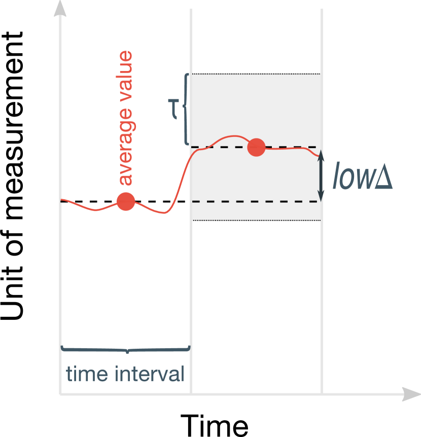
(a) The concept of low$\Delta\textsuperscript{\text{}}\textsubscript{\text{}}$

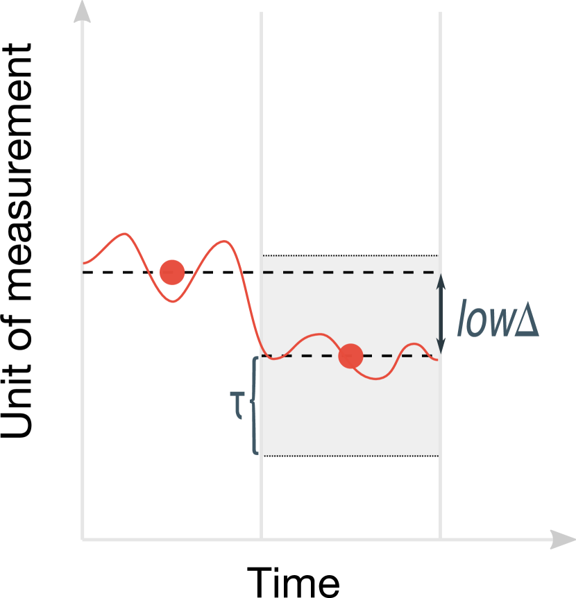
(b) Another case of low$\Delta\textsuperscript{\text{}}\textsubscript{\text{}}$

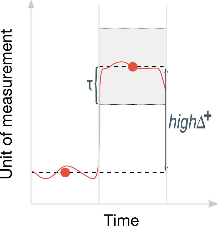
(c) The concept of high$\Delta\textsuperscript{\text{+}}\textsubscript{\text{}}$

(d) The concept of high$\Delta\textsuperscript{\text{-}}\textsubscript{\text{}}$

Figure 2: How the system labels the $\Delta\textsuperscript{\text{}}\textsubscript{\text{}}$s.

Predictions are independent for each metric. Furthermore, any prediction is composed by three factors: the last two symptoms and the last prediction. The general idea is to try to learn the trend and avoid wrong predictions provoked by noise and outliers. Thus, every time that two factors agree in one direction, the prediction is that, in the next interval, the environment will follow it. Otherwise, if the three factors are different, the prediction is that the environment will not undergo variations in the near future. Table 2 shows how we did the predictions using $\Delta\textsuperscript{\text{}}\textsubscript{\text{}}$s.

Last Symptoms		Last Prediction	Prediction
low$\Delta\textsuperscript{\text{}}\textsubscript{\text{}}$	low$\Delta\textsuperscript{\text{}}\textsubscript{\text{}}$	any	low$\Delta\textsuperscript{\text{}}\textsubscript{\text{}}$
high$\Delta\textsuperscript{\text{+}}\textsubscript{\text{}}$	high$\Delta\textsuperscript{\text{+}}\textsubscript{\text{}}$	any	high$\Delta\textsuperscript{\text{+}}\textsubscript{\text{}}$
high$\Delta\textsuperscript{\text{-}}\textsubscript{\text{}}$	high$\Delta\textsuperscript{\text{-}}\textsubscript{\text{}}$	any	high$\Delta\textsuperscript{\text{-}}\textsubscript{\text{}}$
high$\Delta\textsuperscript{\text{+}}\textsubscript{\text{}}$	any	high$\Delta\textsuperscript{\text{+}}\textsubscript{\text{}}$	high$\Delta\textsuperscript{\text{+}}\textsubscript{\text{}}$
high$\Delta\textsuperscript{\text{-}}\textsubscript{\text{}}$	any	high$\Delta\textsuperscript{\text{-}}\textsubscript{\text{}}$	high$\Delta\textsuperscript{\text{-}}\textsubscript{\text{}}$
low$\Delta\textsuperscript{\text{}}\textsubscript{\text{}}$	any	low$\Delta\textsuperscript{\text{}}\textsubscript{\text{}}$	low$\Delta\textsuperscript{\text{}}\textsubscript{\text{}}$
high$\Delta\textsuperscript{\text{+}}\textsubscript{\text{}}$	high$\Delta\textsuperscript{\text{-}}\textsubscript{\text{}}$	low$\Delta\textsuperscript{\text{}}\textsubscript{\text{}}$	low$\Delta\textsuperscript{\text{}}\textsubscript{\text{}}$
high$\Delta\textsuperscript{\text{+}}\textsubscript{\text{}}$	low$\Delta\textsuperscript{\text{}}\textsubscript{\text{}}$	high$\Delta\textsuperscript{\text{-}}\textsubscript{\text{}}$	low$\Delta\textsuperscript{\text{}}\textsubscript{\text{}}$
high$\Delta\textsuperscript{\text{-}}\textsubscript{\text{}}$	low$\Delta\textsuperscript{\text{}}\textsubscript{\text{}}$	high$\Delta\textsuperscript{\text{+}}\textsubscript{\text{}}$	low$\Delta\textsuperscript{\text{}}\textsubscript{\text{}}$

Table 2: How the system reacts to the symptoms.

Finally, if a EG receives information from internal and external sources, each prediction may be based on a different data type. In this case, it combines them in the simplest way: if one of the predictions is labeled as high$\Delta\textsuperscript{\text{}}\textsubscript{\text{}}$, the final prediction is a high$\Delta\textsuperscript{\text{}}\textsubscript{\text{}}$; otherwise, it is a low$\Delta\textsuperscript{\text{}}\textsubscript{\text{}}$.

4.1.1 Adaptive threshold

The value of $\tau\textsubscript{}$ is set based on the proportion of $\Delta\textsuperscript{\text{}}\textsubscript{\text{}}$s seen in the historical data. For example, if the goal is to predict the highest quarter of $\Delta\textsuperscript{\text{}}\textsubscript{\text{}}$s in a day, the threshold will be set at the $75$th percentile of $\Delta\textsuperscript{\text{}}\textsubscript{\text{}}$s. In this case, we identify it with the number $75$ subscripted: $\tau\textsubscript{75}$.

4.1.2 Symptoms

To make those predictions, we must observe the measurements and find symptoms. A symptom, $\sigma\textsubscript{}$, is defined as a value where a $\Delta\textsuperscript{\text{}}\textsubscript{\text{}}>\sigma\textsubscript{}{}$ represents a high probability of having $\Delta\textsuperscript{\text{}}\textsubscript{\text{}}>\tau\textsubscript{}{}$ in the next interval. Therefore, if we notice that the most recent $\Delta\textsuperscript{\text{}}\textsubscript{\text{}}$ is greater than $\sigma\textsubscript{}$, we have a symptom of high$\Delta\textsuperscript{\text{}}\textsubscript{\text{}}$; otherwise, it is a symptom of low$\Delta\textsuperscript{\text{}}\textsubscript{\text{}}$. Even though the concepts of $\sigma\textsubscript{}$ and $\tau\textsubscript{}$ are similar, the numerical values may be different. For example, after observing the historical data, we might notice that every $\Delta\textsuperscript{\text{}}\textsubscript{\text{}}>\tau\textsubscript{40}$ calculated at time $t$ was followed by a $\Delta\textsuperscript{\text{}}\textsubscript{\text{}}>\tau\textsubscript{75}$ at time $t+1$. So, we would set the value of $\sigma\textsubscript{}$ at the $40$th percentile of $\Delta\textsuperscript{\text{}}\textsubscript{\text{}}$s.

5 Evaluation

We considered each measurement done by the real nodes as the average of the network measurements in our simulations. Moreover, each set of measurements done by a node in a day was considered one day’s worth of data. Therefore, we had enough data to simulate $48$ different days. To check the feasibility of using this solution in the presented scenario, we evaluated the energy consumption in OMNeT++ [8] and the calculations about the performance score in Matlab. First, using OMNeT++ and MiXiM [9], we simulated the energy consumption based on TelosB nodes [10] using BMAC [11] as MAC protocol and a flooding routing protocol. In these simulations, the sensor nodes received new plans from the EG${}_{\text{}}$ every $5$ minutes, as explained in Section 3.2. We calculated the average energy consumption on each plan, considering also the energy spent to disseminate the plan changes through the network.

In Matlab, the data from the sensors were split into a training and a validation datasets to avoid overfitting. Each of these datasets was defined by a set of $24$ days that were randomly selected on each run (repeated random sub-sampling validation). The model was fit to the training data, and predictive accuracy was assessed using the validation data. The tests were done over $10$ different combinations of days and the final results were averaged over the splits. In the end, we checked how the system behaved when the plan of Network B was selected using only internal information (relative humidity values), only external information (temperature values) and combining both, and used the energy consumption levels to plot the results.

5.1 Training dataset

After selecting $24$ days for the training dataset, the measured values were used to set three different parameters:

• The value of $\tau\textsubscript{}$ – The threshold that the EG${}_{\text{}}$s must set. It was calculated as explained in 4.1, based on the measurements done during the training days.

• The values of $\sigma\textsubscript{}$s – The system built a table with the values of $p$ based on percentiles, as shown in Figure 3(d). The numerical value of $\sigma\textsubscript{T}$ and $\sigma\textsubscript{RH}$ was the same as the percentiles of $\Delta\textsuperscript{\text{}}\textsubscript{\text{T}}$ and $\Delta\textsuperscript{\text{}}\textsubscript{\text{RH}}$ with the highest value of $p$.

We assumed that the saved energy and the accuracy of the system have similar importance and set the value of $\alpha=0.5$ in Equation 3. Figure 3(a) shows how much energy can be saved based on the thresholds that are used as symptoms of future changes. For example, at the point $(40,20)$, any $\Delta\textsuperscript{\text{}}\textsubscript{\text{RH}}$ over the $40^{\text{th}}$ percentile (i.e., greater than $40\%$ of the values) is considered as a symptom of change, as well as any $\Delta\textsuperscript{\text{}}\textsubscript{\text{T}}$ over the $20^{\text{th}}$ percentile. When a symptom is detected, the EG may launch a plan to produce more measurements in the next time-interval and, consequently, consume more energy. Figure 3(b) shows the total accuracy of the predictions and Figure 3(c) shows how the accuracy of high$\Delta\textsuperscript{\text{}}\textsubscript{\text{}}$s changes depending on the threshold chosen to represent a symptom of changes in the future.

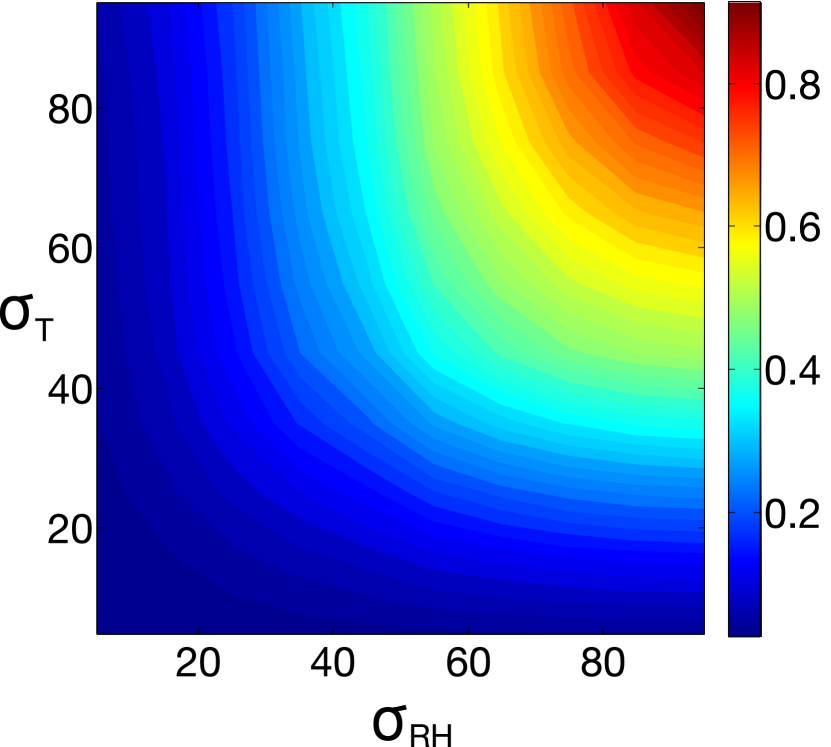
(a) Energy saved ($E_{\text{ps}}$)

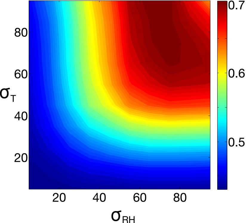
(b) Accuracy of the predictions

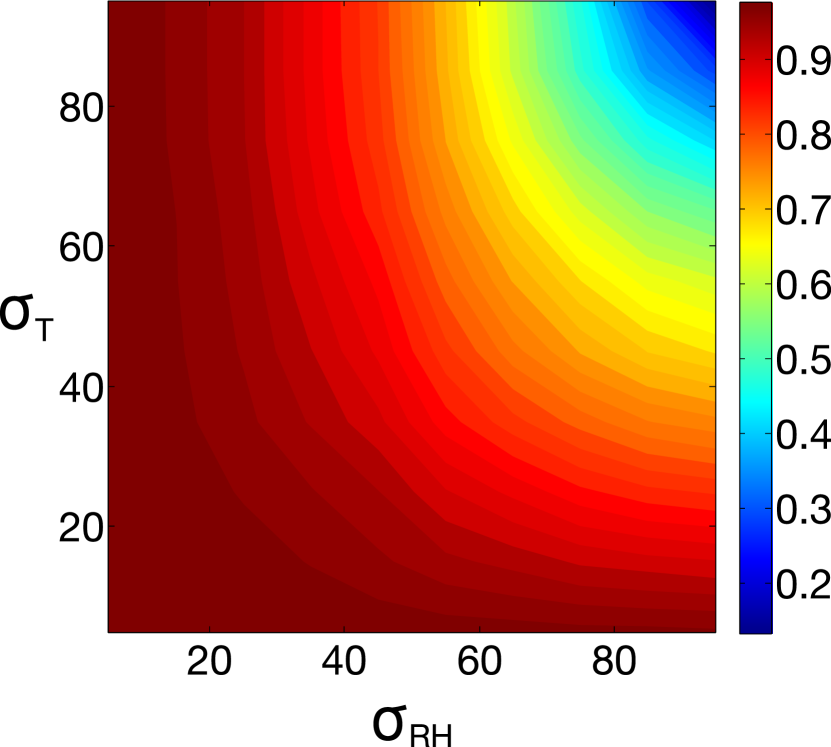
(c) Accuracy of high$\Delta\textsuperscript{\text{}}\textsubscript{\text{}}$s ($P_{\text{$\text{\emph{high}}${$\Delta\textsuperscript{\text{}}\textsubscript{\text{}}$}}}$)

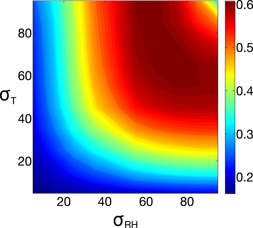
(d) $p_{(0.5)}$

Figure 3: Parameters obtained using the training data.

5.2 Validating dataset

The other $24$ days were considered part of the validating dataset and their data were used to validate whether the system had chosen well and whether our hypothesis was valid. For this, the system used all the parameters calculated in the last step to calculate $p$.

5.3 Results

The plots in Figure 4 show the obtained results, where it is possible to see how much our solution was able to exploit the trade-off between the energy consumption and the quality of the measurements. To show better its benefits, we included two baseline scenarios that did not use collaboration: the first one saved the maximum energy possible by transmitting less measurements; the second did not save energy and always used the plan that transmits more measurements. An important remark is that both scenarios have $p_{(\alpha)}=0$ for any $\alpha$, because either they did not save any energy (the highest consumption plan case) or their accuracy of detecting high$\Delta\textsuperscript{\text{}}\textsubscript{\text{}}$s was zero (the lowest consumption plan case).

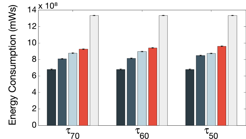
(a) Adaptive sampling.

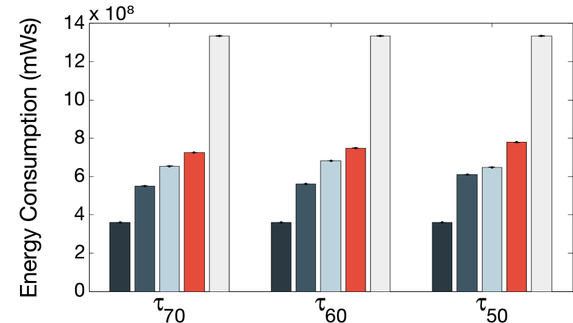
(b) Adaptive sensor nodes selection.

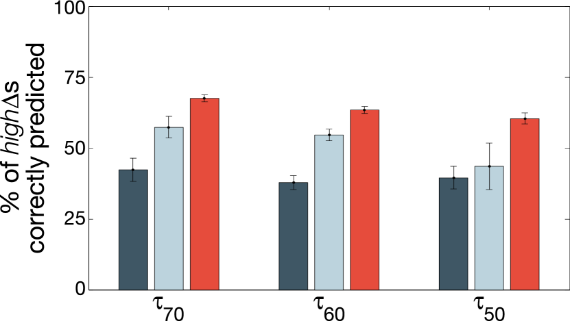
(c) Accuracy of the predictions of high$\Delta\textsuperscript{\text{}}\textsubscript{\text{}}$s.

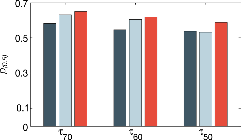
(d) Performance score of each approach.

Figure 4: Simulation results.

The results are split into three groups, according to the $\tau\textsubscript{}$ set for each case ($\tau\textsubscript{70}$, $\tau\textsubscript{60}$ and $\tau\textsubscript{50}$). Each bar represents an average for the $24$ days of the validation dataset. Observing the data, we can see that the correlation between temperature and relative humidity values is closer to $-1$ when we consider only the highest $\Delta\textsuperscript{\text{}}\textsubscript{\text{}}$s, i.e., $\tau\textsubscript{70}$. Therefore, we assume that there are other factors that may influence the small variations in the relative humidity, such as the presence of persons close to the sensors. This explains why the percentage of high$\Delta\textsuperscript{\text{}}\textsubscript{\text{}}$s correctly predicted is lower when the system tries to track a higher number of changes ($\tau\textsubscript{50}$).

In Figures 4(a) and 4(b), we can observe that, when we used only the plan that changed the number of active nodes, the system spent around $54\%$ of the energy compared to the scenario in which the network was always producing more measurements. Also, Figure 4(c) shows that predictions can successfully improve the WSNs’ operation. It is possible to see that, using only the relative humidity values as a reference (absence of external collaboration), $42.3\%$ of the $5$-minute intervals with high$\Delta\textsuperscript{\text{}}\textsubscript{\text{RH}}$s were correctly predicted with $\tau\textsubscript{60}$. Compared to that, we can observe that the energy consumption increased much less than the accuracy levels. For example, with $\tau\textsubscript{60}$, using the combination of internal and external information, the system was able to correctly predict $67.9\%$ more high$\Delta\textsuperscript{\text{}}\textsubscript{\text{}}$s consuming only $33.5\%$ more energy. This means that the energy was used more intelligently in the second case.

Figure 4(d) shows that our approach for inter-WSN information exchange outperforms the other types of collaboration that use less information and spend their energy less efficiently. In summary, the trade-off between energy consumption and QoM was achieved and found to produce more effective results than the other approaches.

6 Conclusion and Future Work

Based on the presented results, it is possible to determine that our mechanism is able to use internal and external information to optimize the WSNs’ performance, which is illustrated by the difference in the values of $p$. During the tests, we have also noticed that these improvements could be achieved only with data that is not only highly correlated, but there must also be a relation of causation between them. In this case, we noticed that changes in temperature led to changes in relative humidity, but the opposite was not necessarily true. Therefore, it would be more complex to make good predictions if we tried to predict temperature changes based on relative humidity values.

Although we made use of real data from existing experiments, we did generic calculations and assumptions that can be extended to numerous scenarios, in order to prove the general idea of this concept. We expect that specific knowledge about different scenarios may lead to better results. For example, as shown in [12], when the relative humidity is over $50\%$, it is possible to calculate its value based on information about the temperature only. Thus, in a scenario similar to ours, the system could save even more energy by letting the EG calculate the local data based on external information.

The next steps include adapt this solution to an autonomic system, as described in [2]. That is, a more generic mechanism which is able to work with other WSN types and is able to work with other prediction methods that may have better performance in different scenarios. Additionally, the idea of an autonomic solution involves a pro-active and self-managing system, which improves the information fusion and the decision optimization, besides creating specific plans for the WSNs according to the predictions about the near future.

References

- [1] Sougata Pal, Simon Oechsner, Boris Bellalta, and Miquel Oliver. Performance optimization of multiple interconnected heterogeneous sensor networks via collaborative information sharing. Journal of Ambient Intelligence and Smart Environments, 5(4):403–413, March 2013.
- [2] Gabriel Martins Dias. Performance optimization of wsns using external information. In World of Wireless, Mobile and Multimedia Networks (WoWMoM), 2013 IEEE 14th International Symposium and Workshops on a, pages 1–2, 2013.
- [3] Falko Dressler, Abdalkarim Awad, and Mario Gerla. Inter-Domain Routing and Data Replication in Virtual Coordinate Based Networks. In 2010 IEEE International Conference on Communications, pages 1–5. IEEE, May 2010.
- [4] Lynne E. Parker. Detecting and monitoring time-related abnormal events using a wireless sensor network and mobile robot. In 2008 IEEE/RSJ International Conference on Intelligent Robots and Systems, pages 3292–3298. IEEE, September 2008.
- [5] Le Borgne Yann-Ael and Gianluca Bontempi. Round Robin Cycle for Predictions in Wireless Sensor Networks. In 2005 International Conference on Intelligent Sensors, Sensor Networks and Information Processing, pages 253–258. IEEE, 2005.
- [6] Amol Deshpande, Carlos Guestrin, Samuel R. Madden, Joseph M. Hellerstein, and Wei Hong. Model-driven data acquisition in sensor networks. In …on Very large data …, pages 588–599, 2004.
- [7] Simon Oechsner, Boris Bellalta, Desislava Dimitrova, and Tobias Hossfeld. Visions and Challenges for Sensor Network Collaboration in the Cloud. In The Seventh International Conference on Innovative Mobile and Internet Services in Ubiquitous Computing, 2014.
- [8] András Varga. The OMNeT++ discrete event simulation system. Proceedings of the European Simulation Multiconference (ESM’2001), 9, 2001.
- [9] A Köpke, M Swigulski, K Wessel, D Willkomm, T E V Parker, P T Kleinhaneveld, T E V Parker, O W Visser, H S Lichte, and S Valentin. Simulating Wireless and Mobile Networks in OMNeT ++ The MiXiM Vision.
- [10] Inc . Crossbow Technology. TelosB Mote Platform. Rev B.
- [11] Khalil Fakih, Jean-Francois Diouris, and Guillaume Andrieux. BMAC: Beamformed MAC protocol with channel tracker in MANET using smart antennas. In 2006 European Conference on Wireless Technologies, volume 2, pages 185–188. IEEE, September 2006.
- [12] Mark G. Lawrence. The Relationship between Relative Humidity and the Dewpoint Temperature in Moist Air: A Simple Conversion and Applications. Bulletin of the American Meteorological Society, 86(2):225–233, February 2005.