Magnetically controlled stellar differential rotation near the transition from solar to anti-solar profiles

Abstract

Context. Late-type stars rotate differentially owing to anisotropic turbulence in their outer convection zones. The rotation is called solar-like (SL) when the equator rotates fastest and anti-solar (AS) otherwise. Hydrodynamic simulations show a transition from SL to AS rotation as the influence of rotation on convection is reduced, but the opposite transition occurs at a different point in the parameter space. The system is bistable, i.e., SL and AS rotation profiles can both be stable.

Aims. We study the effect of a dynamo-generated magnetic field on the large-scale flows, particularly on the possibility of bistable behavior of differential rotation.

Methods. We solve the hydromagnetic equations numerically in a rotating spherical shell that typically covers $\pm 75^{\circ}$ latitude (wedge geometry) for a set of different radiative conductivities controlling the relative importance of convection. We analyze the resulting differential rotation, meridional circulation, and magnetic field and compare the corresponding modifications of the Reynolds and Maxwell stresses.

Results. In agreement with earlier findings, our models display SL rotation profiles when the rotational influence on convection is strong and a transition to AS when the rotational influence decreases. We find that dynamo-generated magnetic fields help to produce SL differential rotation compared to the hydrodynamic simulations. We do not observe any bistable states of differential rotation. In the AS cases we get coherent single-cell meridional circulation, whereas in SL cases we get multi-cellular patterns. In both cases, we obtain poleward circulation near the surface with a magnitude close to that observed in the Sun. In the slowly rotating cases we find activity cycles, but no clear polarity reversals, whereas in the more rapidly rotating cases irregular variations are obtained. Moreover, both differential rotation and meridional circulation have significant temporal variations that are similar in strength to those of the Sun.

Conclusions. Purely hydrodynamic simulations of differential rotation and meridional circulation are shown to be of limited relevance as magnetic fields, self-consistently generated by dynamo action, significantly affect the flows.

1 Introduction

Differential rotation is an important ingredient for the generation of stellar magnetic fields. The internal rotation rate of the Sun has been mapped by helioseismology, revealing that the angular velocity within the convection zone mildly increases (decreases) as a function of radius at low (high) latitudes and that the radial shear is concentrated in shallow layers at the base of the convection zone and near the surface (e.g., Brown et al., 1989; Schou et al., 1998; Thompson et al., 2003). Thus the solar equator rotates faster than its poles. This kind of rotation profile is called solar-like (SL) differential rotation. The opposite case where the equator rotates slower than the poles, is referred to as anti-solar (AS) differential rotation. Due to the difficulties in observing slowly rotating stars that might possess AS differential rotation, it is not clear how common it is in main-sequence stars. However, it has been observed in some K giants (e.g., Strassmeier et al., 2003; Weber et al., 2005; Kovari et al., 2014).

Historically, the differential rotation and magnetic fields of the Sun and other stars have been modeled by two approaches – mean-field models and global convection simulations. In the mean-field approach, small-scale turbulence is parameterized by expressing the Reynolds stress in the momentum equation in terms of the mean velocity, the turbulent electromotive force in the induction equation in terms of the mean magnetic field, and the turbulent heat flux in the entropy equation in terms of the mean entropy. These parameterizations involve turbulent transport coefficients that need to be calculated for highly turbulent flows of stellar interiors. Analytical approaches, such as first-order smoothing, involve approximations that are ill-suited for stellar conditions and may yield inaccurate results. A numerical method for determining the turbulent transport coefficients relevant for the electromotive force is the test-field method (Schrinner et al., 2005, 2007), but for angular momentum or heat transport no similar methods have been developed yet. This means that the turbulent transport coefficients used in mean-field models are often based on educated guesses or they are even used as free parameters. Despite these shortcomings, hydrodynamical mean-field models are capable of producing SL differential rotation (Brandenburg et al., 1992; Kitchatinov & Rüdiger, 1995; Rempel, 2005; Kitchatinov & Olemskoy, 2011) as well as basic properties of the rotation in some other stars (Küker & Rüdiger, 2011; Kitchatinov & Olemskoy, 2011; Hotta & Yokoyama, 2011). However, obtaining AS differential rotation is less straightforward for mean-field models (e.g., Kitchatinov & Rüdiger, 2004). At the same time, mean-field dynamo models also reproduce some features of solar and stellar magnetic cycles either by including turbulent inductive effects (e.g., Käpylä et al., 2006; Pipin & Kosovichev, 2011), or by applying the Babcock-Leighton process in the so-called flux transport dynamo models (e.g., Choudhuri et al., 1995; Dikpati & Charbonneau, 1999; Karak, 2010; Karak et al., 2014; Miesch & Dikpati, 2014).

On the other hand, there have been some successes in modelling the differential rotation and magnetic fields using global convection simulations, mainly in recent years (Miesch et al., 2006; Ghizaru et al., 2010; Racine et al., 2011; Käpylä et al., 2012, 2013; Augustson et al., 2013; Warnecke et al., 2013). However, due to the extreme parameter regimes of the Sun, realistic simulations are not possible at present. Nevertheless, the simulations are able to reproduce solar values of the Coriolis number ${\rm Co}$, which measures the relative importance of rotation and turbulent convection. For certain values of ${\rm Co}$, but with different values for other parameters such as the fluid and magnetic Reynolds and Prandtl numbers, simulations occasionally produce AS differential rotation (e.g., Matt et al., 2011; Käpylä et al., 2014), poleward migration of the large-scale magnetic fields (Gilman, 1983; Käpylä et al., 2010b; Nelson et al., 2013), no clear magnetic cycles (Brown et al., 2010), or sometimes even no appreciable large-scale contribution to the magnetic field (Brun et al., 2004).

According to mean-field hydrodynamics, differential rotation is generated from the anisotropy of the Reynolds stress which is parameterized in terms of the so-called $\Lambda$-effect (Rüdiger, 1980, 1989). A radially increasing (SL) angular velocity results if horizontal turbulent velocities dominate over vertical ones, while AS rotation follows if radial motions (even laminar ones) are dominant. The importance of the $\Lambda$-effect depends on the rotational influence on the turbulence, i.e., the value of ${\rm Co}$, which is the ratio of the convective turnover time to the rotation period. At large ${\rm Co}$, the SL rotation is more favorable and the transition from SL to AS rotation depends on the Coriolis number (Brun & Palacios, 2009; Chan, 2010; Käpylä et al., 2011a, b; Guerrero et al., 2013; Gastine et al., 2013, 2014). Using Boussinesq convection, Gastine et al. (2014) discovered that near the transition from AS to SL rotation, both states are possible, depending on the initial conditions of the simulations. This has been independently verified by Käpylä et al. (2014) in fully compressible convection simulations. If this discovery were to apply to the Sun, this might have important consequences, because young rapidly rotating stars, which preferably possess SL rotation, slowly spin down due to loss of the angular momentum and can persist in the SL rotation state even when their rotation is slow. Some doubts have already been expressed by Fan & Fang (2014), who found that the bistability disappears when magnetic fields are present.

In the magnetohydrodynamic case the situation is more complicated than in the case of pure hydrodynamics. A dynamically significant magnetic field, which possibly varies cyclically, introduces extra time dependent effects into the system, capable of influencing the fluid flow both through large-scale effect (Malkus-Proctor effect; see Malkus & Proctor, 1975; Brandenburg et al., 1992) and small-scale effects (Reynolds and Maxwell stresses and therefore the $\Lambda$-effect; see Kitchatinov et al., 1994). Therefore, the magnetic field tries to destabilize the equilibrium states of the rotation. To explore to what extent the presence of a dynamically significant large-scale magnetic field affects the bistable nature of the differential rotation we perform several simulations with the same setup as in Käpylä et al. (2014), but including magnetic fields. Similar to their work, we perform two types of simulations. In one of them we run the simulations from scratch, i.e., with an initially rigid rotation profile. Then we take either a SL state or an AS state and vary the rotational influence by varying the radiative heat conductivity to identify the transition. We analyse the activity cycles using diagnostic tools of stellar activity in Sect. 3.7. Next we measure the temporal variations of the Lorentz forces (both from large-scale and small-scale contributions) to understand the temporal variations of the large-scale flows observed in the simulations (Sect. 3.8). Finally, we compute the contributions of Reynolds stress, Maxwell stress, and the stresses from the azimuthally averaged mean flow and mean magnetic field to the angular momentum balance (Sect. 4). Then we study the influence of the magnetic field on the angular momentum transport by comparing the results with the hydrodynamic simulations.

2 The Model

2.1 Basic equations

Our model is similar to many earlier studies (Käpylä et al., 2012, 2013; Cole et al., 2014). The hydrodynamic part of this model has been used in Käpylä et al. (2014). We model a spherical wedge with radial, latitudinal, and longitudinal extents $r_{0}\leq r\leq r_{1}$, $\theta_{0}\leq\theta\leq\pi-\theta_{0}$, and $0\leq\phi\leq\phi_{0}$, respectively. Here, $r_{0}=0.72\,R_{\odot}$ and $r_{1}=0.97\,R_{\odot}$ are the positions of the bottom and top of the computational domain, $R_{\odot}$ is the radius of the Sun, $\theta_{0}=\pi/12$ is the colatitude of the polar cap, and $\phi_{0}=\pi/2$ is the longitudinal extent. The following hydromagnetic equations are solved.

$$\frac{\partial\bm{A}}{\partial t}={\bm{u}}\times{\bm{B}}-\mu_{0}\eta{\bm{J}},$$ (1)

$$\frac{D\ln\rho}{Dt}=-\bm{\nabla}\cdot\bm{u},$$ (2)

$$\frac{D\bm{u}}{Dt}=\bm{g}-2\bm{\Omega}_{0}\times\bm{u}+\frac{1}{\rho}\left(\bm{J}\times\bm{B}+\bm{\nabla}\cdot 2\nu\rho\bm{\mathsf{S}}-\bm{\nabla}p\right),$$ (3)

$$T\frac{Ds}{Dt}=-\frac{1}{\rho}\bm{\nabla}\cdot\left({\bm{F}^{\rm rad}}+{\bm{F}^{\rm SGS}}\right)+2\nu\bm{\mathsf{S}}^{2}+\frac{\eta\mu_{0}}{\rho}\bm{J}^{2},$$ (4)

where ${\bm{A}}$ is the magnetic vector potential, ${\bm{B}}=\bm{\nabla}\times{\bm{A}}$ is the magnetic field, ${\bm{J}}=\bm{\nabla}\times{\bm{B}}/\mu_{0}$ is the current density with $\mu_{0}$ being the vacuum permeability, $\bm{u}$ is the velocity, $D/Dt=\partial/\partial t+\bm{u}\cdot\bm{\nabla}$ is the advective derivative, $\rho$ is the density, $s$ is the specific entropy, $T$ is the temperature, $p$ is the pressure, $\nu$ is the constant kinematic viscosity, $\bm{g}=-GM_{\odot}\bm{r}/r^{3}$ is the gravitational acceleration with $M_{\odot}$ being the mass of the Sun, $\bm{\Omega}_{0}=(\cos\theta,-\sin\theta,0)\Omega_{0}$ is the angular velocity vector, $\mathsf{S}_{ij}={\textstyle{1\over 2}}(u_{i;j}+u_{j;i})-{\textstyle{1\over 3}}\delta_{ij}\bm{\nabla}\cdot\bm{u}$ is the rate of strain tensor, where the semicolons denote covariant differentiation. The radiative and subgrid scale (SGS) heat fluxes are given by

$${\bm{F}^{\rm rad}}=-K\bm{\nabla}T\quad\mbox{and}\quad{\bm{F}^{\rm SGS}}=-\chi_{\rm SGS}\rho T\bm{\nabla}s,$$ (5)

respectively. Here $K$ is the radiative heat conductivity and $\chi_{\rm SGS}$ is the turbulent heat diffusivity. The latter represents the unresolved convective transport of heat (Käpylä et al., 2013). The fluid obeys the ideal gas law $p=(\gamma-1)\rho e$, where $\gamma=c_{\rm P}/c_{\rm V}=5/3$ is the ratio of specific heats at constant pressure and volume, and $e=c_{\rm V}T$ is the specific internal energy.

2.2 Initial and boundary conditions

The initial hydrostatic state is isentropic, so the temperature is given by

$$\frac{\partial T}{\partial r}=-\frac{GM_{\odot}/r^{2}}{c_{\rm V}(\gamma-1)(n_{\rm ad}+1)},$$ (6)

where $n_{\rm ad}=1.5$ is the polytropic index and the value of $\partial T/\partial r$ at $r=r_{0}$ is fixed. The density stratification follows from hydrostatic equilibrium. The initial state chosen is not in thermodynamic equilibrium but closer to the final convecting state to reduce the needed computational time to reach a thermally relaxed state. The heat conductivity profile is chosen such that radiative diffusion is responsible for supplying the energy flux into the system. Radiative diffusion becomes progressively less efficient toward the surface (Käpylä et al., 2011a). As in Käpylä et al. (2013, 2014), this is achieved by taking a depth-dependent polytropic index $n(r)=\delta n(r/r_{0})^{-15}+n_{\rm ad}-\delta n$ for the radiative conductivity $K(r)=K_{0}[n(r)+1]$, where the reference conductivity is $K_{0}=(\mathcal{L}/4\pi)c_{\rm V}(\gamma-1)(n_{\rm ad}+1)\rho_{0}\sqrt{GM_{\odot}R_{\odot}}$, with $\mathcal{L}$ being the non-dimensional luminosity. Note that $n=n_{\rm ad}$ at the bottom and $n\to$ $n_{\rm ad}-\delta n$ towards the surface. Hence, $K$ decreases toward the surface like $r^{-15}$ such that the value of $\delta n$ regulates the flux that is carried by convection (Brandenburg et al., 2005; Käpylä et al., 2014).

Along with the imposed energy flux at the bottom boundary $F_{\rm b}=-(K\partial T/\partial r)_{r=r_{0}}$, the values of $\Omega_{0}$, $\nu$, $\eta$, and $\overline{\chi}_{\rm SGS}=\chi_{\rm SGS}$ at the middle of the convection zone $r=r_{\rm m}=0.845\,R_{\odot}$ are defined. The turbulent heat conductivity $\chi_{\rm SGS}$ is piecewise constant above $r>0.75R_{\odot}$ with $\chi_{\rm SGS}=\overline{\chi}_{\rm SGS}$ in $0.75R_{\odot}<r<0.95R_{\odot}$, and $\chi_{\rm SGS}=1.35\overline{\chi}_{\rm SGS}$ at $r\geq 0.95R_{\odot}$. At $r<0.75R_{\odot}$, $\chi_{\rm SGS}$ tends smoothly to zero (see Fig. 1 of Käpylä et al., 2011a). We fix $\chi_{\rm SGS}$ in such a way that at $r=r_{1}$ it corresponds to $5\times 10^{8}\,{\rm m}^{2}\,{\rm s}^{-1}$ in physical units. We also assume the density and temperature at $r=r_{0}$ to have solar values, $\rho_{0}=200$ kg m^-3 and $T_{0}=2.23\times 10^{6}$ K.

Radial and latitudinal boundaries are assumed to be impenetrable and stress free for the flow, whereas for the magnetic field we assume a radial field condition on the outer radial boundary and perfect conductor conditions on the lower radial and latitudinal boundaries; see Käpylä et al. (2013) for details. Density and entropy have vanishing first derivatives on the latitudinal boundaries. A black body condition with $\sigma T^{4}=-K\nabla_{r}T-\chi_{\rm SGS}\rho T\nabla_{r}s,$ where $\sigma$ is related to the Stefan–Boltzmann constant, is applied on the upper radial boundary. However the value of $\sigma$ is modified to attain the desired values of surface temperature and energy flux. Moreover, we choose $\sigma$ in such a way that in the initial non-convecting state the flux at the surface carries the total luminosity through the boundary. We use small-scale low amplitude Gaussian noise as initial condition for the velocity and magnetic fields.

As discussed by Käpylä et al. (2013, 2014), in our fully compressible simulation the time step is severely limited if we were to use the solar luminosity. This would imply both huge Rayleigh and small Mach numbers. This problem is avoided by taking an about $10^{6}$ times higher luminosity in the simulation than in the Sun. However, the convective velocity $u$ becomes then in our simulation 100 times larger than in the Sun because the convective energy flux $F_{\rm conv}$ scales as $\rho u^{3}$. Therefore to achieve the same rotational influence on the flow as in the Sun, we need to increase $\Omega$ by the same factor. Consequently, we have the relations: $\Omega_{\rm sim}=(L_{0}/L_{\odot})^{1/3}\Omega_{\odot}\quad{\rm and}\quad{\bm{u}}_{\rm sim}=(L_{0}/L_{\odot})^{1/3}{\bm{u}}_{\odot},$ where $L_{0}$ is the luminosity in simulation, $L_{\odot}\approx 3.84\times 10^{26}$ W is the solar luminosity, and $\Omega_{\odot}$ is the average solar rotation rate $\approx 2.7\times 10^{-6}$ s^-1. This allows us to quote values for angular velocity, meridional circulation, and magnetic field in physical units that can be compared with solar values and with results of other groups. However, we often quote ratios between different quantities that are obviously non-dimensional and therefore not affected. All computations are performed with the Pencil Code.

2.3 Dimensionless parameters and diagnostics

First, we define the non-dimensional input parameters. The luminosity parameter $\mathcal{L}$ and the normalized pressure scale height at the surface $\xi$ are given by

$$\mathcal{L}=\frac{L_{0}}{\rho_{0}(GM_{\odot})^{3/2}R_{\odot}^{1/2}},\quad\xi=\frac{(\gamma-1)c_{\rm V}T_{1}}{GM_{\odot}/R_{\odot}},$$ (7)

where $T_{1}$ is the temperature at the surface. The influence of rotation is measured by the Taylor number,

$${{\rm Ta}=(2\Omega_{0}\Delta r^{2}/\nu)^{2},}$$ (8)

where $\Delta r=r_{1}-r_{0}$ is the thickness of the convecting shell. The fluid, magnetic, and SGS Prandtl numbers are defined as

$${\rm Pr}=\frac{\nu}{\chi_{\rm m}},\quad{\rm Pm}=\frac{\nu}{\eta},\quad{\rm Pr}_{\rm SGS}=\frac{\nu}{\overline{\chi}_{\rm SGS}},$$ (9)

respectively, where $\chi_{\rm m}=K(r_{\rm m})/c_{\rm P}\rho_{\rm m}$ is the thermal diffusivity and $\rho_{\rm m}$ is the density, both evaluated $r=r_{\rm m}$. Furthermore, we define the non-dimensional viscosity,

$$\tilde{\nu}=\frac{\nu}{\sqrt{GM_{\odot}R_{\odot}}},$$ (10)

and the Rayleigh and convective Rossby numbers (Gilman, 1977),

$${\rm Ra}\!=\!\frac{GM_{\odot}(\Delta r)^{4}}{\nu\overline{\chi}_{\rm SGS}R_{\odot}^{2}}\bigg{(}\!-\frac{1}{c_{\rm P}}\frac{{\rm d}s}{{\rm d}r}\!\bigg{)}_{r_{\rm m}}\!\!,\ \ {\rm Ro}_{\rm c}=\left(\frac{{\rm Ra}}{{\rm Pr}_{\rm SGS}{\rm Ta}}\right)^{1/2}\!\!,\;\;\;$$ (11)

where the entropy gradient of the non-convecting hydrostatic solution is evaluated in the middle of the convection zone, $r=r_{\rm m}$. We also quote the initial density contrast $\Gamma_{\rho}^{(0)}\equiv\rho(r_{0})/\rho(r_{1})$.

As diagnostic quantities we define the fluid and magnetic Reynolds numbers, and the Coriolis number as

$${\rm Re}=\frac{u_{\rm rms}}{\nu k_{\rm f}},\quad{\rm Rm}=\frac{u_{\rm rms}}{\eta k_{\rm f}}={\rm Pm}{\rm Re},\quad{\rm Co}=\frac{2\Omega_{0}}{u_{\rm rms}k_{\rm f}},$$ (12)

where $u_{\rm rms}=\sqrt{(3/2)\langle u_{r}^{2}+u_{\theta}^{2}\rangle_{r\theta\phi t}}$ is the volume and time averaged rms velocity during the time when the simulation is thermally relaxed. We exclude $u_{\phi}$ from $u_{\rm rms}$ as it is dominated by the differential rotation, and use $k_{\rm f}=2\pi/\Delta r$ as an estimate of the wavenumber of the largest eddies. The Taylor number can also be written as ${\rm Ta}={\rm Co}^{2}{\rm Re}^{2}(k_{\rm f}R_{\odot})^{4}$.

We define mean values as averages over longitude and time and denote these by an overbar. Sometimes we also perform additional averaging over latitude and/or radius which we always mention explicitly.

Table 1: Summary of the runs.

$$\begin{array}[]{p{0.05\linewidth}ccccccrrccccccl}\hline\cr\vskip 3.0pt plus 1.0pt minus 1.0pt\cr Run&{\rm Ra}&{\rm Pr}&\delta n&{\rm Ro}_{\rm c}&{\rm Re}&{\rm Co}&\Delta_{\Omega}^{(\theta)}&\Delta_{\Omega}^{(r)}&\tilde{E}_{\rm kin}[10^{-7}]&E_{\rm mer}/E_{\rm kin}&E_{\rm rot}/E_{\rm kin}&\tilde{L}_{\rm rad}&\tilde{L}_{\rm conv}&{\rm DR}&{\rm{\color[rgb]{0,0,0}activity\leavevmode\nobreak\ cycle}}\\ \hline\cr A&3.93\cdot 10^{5}&39.9&2.5&0.73&33&1.34&-0.184&-0.185&0.25&3.77\times 10^{-3}&0.173&0.09&0.95&{\rm AS}&{\rm{\color[rgb]{0,0,0}fairly}\leavevmode\nobreak\ regular}\\ B&3.54\cdot 10^{5}&20.3&2.25&0.69&32&1.35&-0.158&-0.143&0.24&2.87\times 10^{-3}&0.134&0.19&0.84&{\rm AS}&{\rm{\color[rgb]{0,0,0}fairly}\leavevmode\nobreak\ regular}\\ BC&3.54\cdot 10^{5}&15.6&2.1&0.67&32&1.38&-0.151&-0.134&0.23&2.69\times 10^{-3}&0.155&0.24&0.77&{\rm AS}&{\rm{\color[rgb]{0,0,0}fairly}\leavevmode\nobreak\ regular}\\ C&3.16\cdot 10^{5}&13.6&2.0&0.65&30&1.44&0.033&0.014&0.27&1.05\times 10^{-3}&0.341&0.28&0.70&{\rm SL}&{\rm intermittent}\\ D&2.92\cdot 10^{5}&11.3&1.85&0.63&26&1.67&0.118&0.059&0.26&0.67\times 10^{-3}&0.487&0.33&0.57&{\rm SL}&{\rm irregular}\\ E&2.77\cdot 10^{5}&10.2&1.75&0.61&25&1.75&0.111&0.057&0.23&0.81\times 10^{-3}&0.468&0.37&0.52&{\rm SL}&{\rm irregular}\\ \hline\cr D0&2.92\cdot 10^{5}&11.3&1.85&0.63&26&1.67&0.118&0.059&0.26&0.67\times 10^{-3}&0.487&0.33&0.57&{\rm SL}&{\rm irregular}\\ D1&3.16\cdot 10^{5}&13.6&2.00&0.65&30&1.46&0.013&0.008&0.29&1.53\times 10^{-3}&0.333&0.28&0.71&{\rm SL}&{\rm irregular}\\ D2&3.31\cdot 10^{5}&15.7&2.10&0.67&31&1.40&-0.069&-0.074&0.21&1.70\times 10^{-3}&0.121&0.24&0.76&{\rm AS}&{\rm irregular}\\ D3&3.47\cdot 10^{5}&18.5&2.20&0.68&32&1.38&-0.153&-0.140&0.23&2.69\times 10^{-3}&0.143&0.20&0.81&{\rm AS}&{\rm{\color[rgb]{0,0,0}fairly}\leavevmode\nobreak\ regular}\\ D4&3.62\cdot 10^{5}&22.5&2.30&0.70&32&1.36&-0.167&-0.158&0.24&3.17\times 10^{-3}&0.149&0.17&0.86&{\rm AS}&{\rm{\color[rgb]{0,0,0}fairly}\leavevmode\nobreak\ regular}\\ \hline\cr A0&3.93\cdot 10^{5}&39.9&2.5&0.73&33&1.34&-0.184&-0.185&0.25&3.77\times 10^{-3}&0.173&0.09&0.95&{\rm AS}&{\rm{\color[rgb]{0,0,0}fairly}\leavevmode\nobreak\ regular}\\ A1&3.85\cdot 10^{5}&33.3&2.45&0.72&32&1.36&-0.172&-0.184&0.25&3.57\times 10^{-3}&0.163&0.11&0.92&{\rm AS}&{\rm{\color[rgb]{0,0,0}fairly}\leavevmode\nobreak\ regular}\\ A2&3.78\cdot 10^{5}&28.5&2.4&0.71&32&1.36&-0.135&-0.144&0.23&2.93\times 10^{-3}&0.122&0.13&0.89&{\rm AS}&{\rm irregular}\\ A3&3.62\cdot 10^{5}&22.3&2.3&0.70&32&1.38&-0.154&-0.150&0.23&2.95\times 10^{-3}&0.126&0.17&0.85&{\rm AS}&{\rm irregular}\\ A4&3.47\cdot 10^{5}&18.3&2.2&0.68&32&1.38&-0.141&-0.133&0.23&2.79\times 10^{-3}&0.124&0.20&0.81&{\rm AS}&{\rm irregular}\\ A5&3.31\cdot 10^{5}&15.5&2.1&0.67&31&1.41&-0.075&-0.073&0.23&2.04\times 10^{-3}&0.142&0.24&0.76&{\rm AS}&{\rm irregular}\\ A6&3.16\cdot 10^{5}&13.4&2.0&0.65&30&1.44&0.066&0.017&0.24&1.40\times 10^{-3}&0.212&0.28&0.71&{\rm SL}&{\rm irregular}\\ A7&3.00\cdot 10^{5}&11.9&1.9&0.63&29&1.53&0.091&0.055&0.31&0.58\times 10^{-3}&0.499&0.31&0.62&{\rm SL}&{\rm irregular}\\ A8&2.85\cdot 10^{5}&10.7&1.8&0.62&27&1.61&0.121&0.073&0.29&0.61\times 10^{-3}&0.553&0.35&0.54&{\rm SL}&{\rm irregular}\\ \hline\cr B${}^{\prime}$&3.54\cdot 10^{5}&20.3&2.25&0.69&32&1.34&-0.154&-0.149&0.21&3.66\times 10^{-3}&0.117&0.19&0.82&{\rm AS}&{\rm fairly\leavevmode\nobreak\ regular}\\ B${}^{\prime\prime}$&3.54\cdot 10^{5}&20.3&2.25&0.69&32&1.36&-0.132&-0.140&0.25&2.66\times 10^{-3}&0.128&0.19&0.85&{\rm AS}&{\rm fairly\leavevmode\nobreak\ regular}\\ \hline\cr\end{array}$$

3 Results

First, we perform a set of simulations for different values of the radiative conductivity starting from the initial condition described in Sect. 2.2. These are referred to as Runs A–E in Table 1. Except for the allowance of a magnetic field, all other input parameters of our Runs A–E are identical to those of Käpylä et al. (2014). However, we have an additional Run BC in this set, whose radiative conductivity lies between those of Runs B and C. It turns out that Runs A–BC produce AS differential rotation, while Runs C–E produce SL differential rotation. Next, we perform two further sets of runs where we use Runs A and D with AS and SL differential rotation, respectively, as progenitors to study the possibility of bistability of the rotation profile.

3.1 Energy fluxes in our dynamo runs

The radiative conductivity in our model is controlled by the parameter $\delta n$, regulating the fractional flux that convection has to transport. Increasing $\delta n$ reduces the radiative flux and increases the convective flux and thus $u_{\rm rms}$. Having $\Omega_{0}$ fixed, changing $\delta n$ affects the rotational influence on the convection via the convective velocities (for further details see Käpylä et al., 2014). Hence, different values of $\delta n$ in Runs A–E imply different values of ${\rm Co}$. Thus, Run E is more rotationally dominated than Run A. For Run A with $\delta n=2.5$, the convective flux dominates over the other fluxes and the radiative flux transports a very small fraction of the luminosity. For the definitions of the fluxes we refer to Eqs. (26)–(31) of Käpylä et al. (2013).

In the statistically stationary state, the total luminosity $L_{\rm tot}(r)=4\pi r^{2}{\cal F}_{\rm tot}(r)$ is constant, where ${\cal F}_{\rm tot}$ is the time averaged total energy flux. In Fig. 1 we show the radial dependence of the contributions from radiation ($L_{\rm rad}$) and convection ($L_{\rm conv}$), as well as kinetic ($L_{\rm kin}$), viscous ($L_{\rm visc}$), and subgrid scale ($L_{\rm SGS}$) energy fluxes in the convection zone for Runs A and E. For comparison we also show the fluxes from the corresponding hydrodynamic simulations of Käpylä et al. (2014) with red lines. We see that for Run A, the convective, kinetic, and SGS energy fluxes have decreased in the lower part of the convection zone in the magnetic case. In Run E there is very little change in the SGS flux and only a small reduction of the convective and kinetic energy fluxes is visible. In Table 1 we show the fractions of the radiative and the convective fluxes at the middle of the convection zone for all the runs. In Runs A, B, and BC, the convective flux is above $75\%$ and the radiative flux is less than $25\%$. By contrast, Runs C, D, and E have a convective flux of less than $70\%$ and the radiative flux is larger than $25\%$.

We find that the rms-velocity is compatible with a one-third power proportionality to the convective energy flux – at least in the narrow range of parameters studied here; see Fig. 2. This is in agreement with the scaling used in connection with the artificially high luminosities used in our simulations (see also Brandenburg et al., 2005).

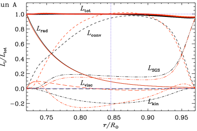
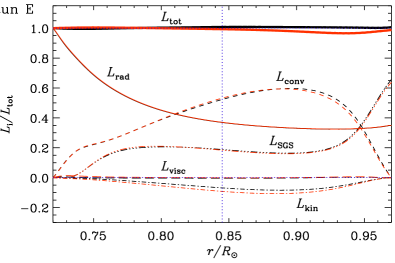
Figure 1: The contributions of different energy fluxes of Runs A (top) and E (bottom). The black (red) lines correspond to magnetohydrodynamic (hydrodynamic) case. Thin solid: radiative, dashed: convective, long dashed: viscous, dash-dotted: kinetic energy, dash-triple-dotted: SGS, and thick solid: total. Dotted horizontal lines indicate the zero and unity values. The blue vertical dotted line indicates the position of the middle of the convection zone $r=r_{\rm m}$.

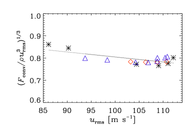
Figure 2: Variation of ${(F_{\rm conv}/\rho u_{\rm rms}^{3})}^{1/3}$ averaged over the whole convection zone as a function of $u_{\rm rms}$ from different runs. Black asterisks: Runs A–E, red diamonds: Runs E1–E4, and blue triangles: Runs A1–A8. The dotted line shows the linear dependence between $u_{\rm rms}$ and ${(F_{\rm conv}/\rho u_{\rm rms}^{3})}^{1/3}$.

3.2 Differential rotation

In Fig. 3 we show the rotation profile $\overline{\Omega}=\overline{u}_{\phi}/r\sin\theta+\Omega_{0}$ for Runs A–E. We see that in Runs A, B, and BC the equator rotates slower than the mid- and high latitudes which is opposite to the rotation profile observed in the Sun. However, we find that the regions near the latitudinal boundaries have slower rotation than mid-latitudes, which was not observed in the hydrodynamical simulations of Käpylä et al. (2014). We have repeated Run B by increasing and decreasing the extent of the latitudinal boundaries. Runs B^′ and B^′′ in Table 1 correspond to these two cases where the latitudinal end points are at $\pm 84^{\circ}$ and $\pm 66^{\circ}$, respectively. In Fig. 4, we show $\overline{\Omega}$ profiles for these two runs, whereas in Fig. 5 we show their latitudinal variations at $r=0.96R_{\odot}$. From these two plots we see that the rotation profiles are very similar in all these runs up to about $\pm 50^{\circ}$ latitudes and the significant departures appear only near the boundaries. However, the slowly rotating high-latitude branch still exists in all runs. Therefore this is probably not due to our restricted latitudinal extent, but may be a real feature which might be caused by the magnetic fields.

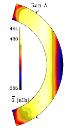
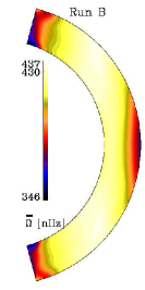
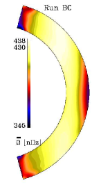
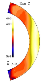
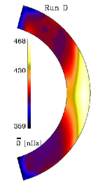
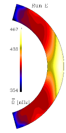
Figure 3: The distribution of angular velocity (in nHz) $\overline{\Omega}$ in the meridional plane from Runs A–E. $\overline{\Omega}$ is computed from $\Omega$ first by the longitudinal average and then the time average over the last few cycles. The arrows in the leftmost panel show the co-latitudes at which the latitudinal differential rotation is computed in Eq. (13).

By comparing the rotation profiles from hydrodynamic simulations of Käpylä et al. (2014) for Runs A–E, we see that the pole–equator differential rotation is generally weaker in the magnetic runs, the reduction being strongest in the runs with a slowly rotating equator. This will be discussed in Sect. 3.5, where we give the ratio of the rotational energy of the hydrodynamic and magnetic simulations. The overall reduction of the pole–equator differential rotation by magnetic fields agrees with what has been reported before (e.g., Brun et al., 2004; Beaudoin et al., 2013; Fan & Fang, 2014). In particular, for slow rotation Fan & Fang (2014) found a switch from AS to SL differential rotation, which agrees with our results reported below. By contrast, Brun et al. (2004) and Beaudoin et al. (2013) only consider runs with SL rotation, but in the models by Brun et al. (2004) the angular velocity at high latitudes is not much reduced by magnetic fields. In the models of Beaudoin et al. (2013), on the other hand, there is a lower overshoot layer, where angular velocity is constant and equal to that at high latitudes when there is a magnetic field. This is, however, not the case in their non-magnetic runs, so the magnetic field leads to a strong reduction in their case, which is similar to ours, but different from what Brun et al. (2004) found, although comparing runs with and without overshoot layers can be misleading due to different physical effects involved.

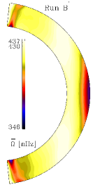
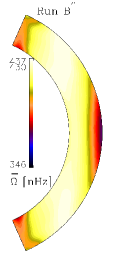
Figure 4: Same as Run B in Fig. 3, but here the latitudinal extent is different. For the left panel the latitudinal boundaries are at $\pm 84^{\circ}$, whereas for the right one they are at $\pm 66^{\circ}$.

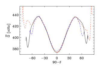
Figure 5: Variations of angular velocities $\overline{\Omega}$ at $r=0.96R_{\odot}$ from Runs B (solid line), B^′ (red dashed), and B^′′ (blue dash-dotted).

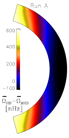
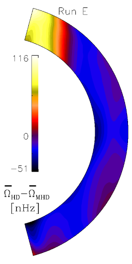
Figure 6: Difference of $\overline{\Omega}$ between the HD and MHD runs. The left and right panels are for Runs A and E, respectively.

To illustrate the reduction of differential rotation in our magnetic runs, we show in Fig. 6 the differences in $\overline{\Omega}$ between the hydrodynamic and magnetic versions of Runs A and E. We see that for Run A the difference is even larger than the average rotation rate of the Sun. Possible reasons for the reduction of differential rotation will be discussed in Sect. 4.

In Runs C–E, the equator rotates faster than the polar regions, as is also the case in the Sun. However, unlike some of the non-magnetic solar-like cases of Käpylä et al. (2014), we never obtain polar vortices or jet-like structures with magnetic fields. It is also interesting to note that the pole–equator difference in the rotational velocity is comparable to that of the Sun. The solar value ($\sim$ 430 nHz) is marked in each colorbar of Fig. 3.

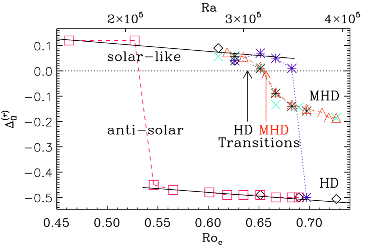
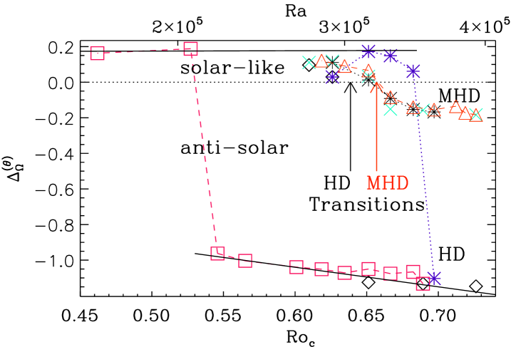
Figure 7: Radial (left panel) and latitudinal (right panel) differential rotation, defined by Eq. (13), for Runs A–E (green crosses), A0-A8 (red dashed line with triangles), and D0-D4 (black asterisks with dotted line). The other points are taken from the hydrodynamical simulations (black diamonds: Runs A–E, blue dotted line with asterisks: Runs D0–D4, and red dashed line with squares: Runs B0–B10) of Käpylä et al. (2014). The horizontal black dotted lines show the zero value. A red (black) arrow shows the transition point when differential rotation in the MHD (HD) simulations changes from AS to SL rotation with the decrease of ${\rm Ro}_{\rm c}$.

3.3 Identifying the SL to AS transition

We measure the relative radial and latitudinal differential rotation by the quantities

$$\Delta_{\Omega}^{(r)}=\frac{\Omega_{\rm eq}-\Omega_{\rm bot}}{\Omega_{\rm eq}},\quad\Delta_{\Omega}^{(\theta)}=\frac{\Omega_{\rm eq}-\Omega_{55}}{\Omega_{\rm eq}},$$ (13)

where $\Omega_{\rm eq}=\overline{\Omega}(r_{1},\pi/2)$ and $\Omega_{\rm bot}=\overline{\Omega}(r_{0},\pi/2)$ are the equatorial rotation rates at the surface and at the base of the convection zone, and $\Omega_{55}={\textstyle{1\over 2}}[\overline{\Omega}(r_{1},35^{\circ})+\overline{\Omega}(r_{1},145^{\circ})]$ is the rotation rate at latitudes $\pm 55\degr$ computed as an average of $\overline{\Omega}$ at $35^{\circ}$ and $145^{\circ}$ co-latitudes on the outer radius. The arrows in the left panel of Fig. 3 show the positions of these points in the $r$-$\theta$ plane. The values of $\Delta_{\Omega}^{(r)}$ and $\Delta_{\Omega}^{(\theta)}$, listed in Table 1, help us to identify AS and SL differential rotation. SL differential rotation implies $\Delta_{\Omega}^{(r)}>0$ and $\Delta_{\Omega}^{(\theta)}>0$. Following this definition we see that Runs A, B, and BC are classified as AS and Runs C–E as SL. Hence we see that there is a transition from AS to SL rotation around ${\rm Co}\sim 1.4$. Although this transition has been reported extensively in the literature (Gilman, 1977; Rieutord et al., 1994; Käpylä et al., 2011b; Gastine et al., 2013; Guerrero et al., 2013), the possibility of a bistability has only recently been discovered (Gastine et al., 2014; Käpylä et al., 2014), i.e., AS and SL rotation profiles can be obtained for the same input parameters. By comparing the current results with the hydrodynamical ones, we see that the transition happens at a slightly larger value of ${\rm Ro}_{\rm c}$, also manifested by the change of the AS hydrodynamical counterpart of Run C, to SL in the MHD regime. The transition observed in the current dynamo cases is less abrupt than that of earlier hydrodynamic studies. Therefore we conclude that the magnetic field helps to produce SL differential rotation, which has also been found in the recent anelastic simulations of Fan & Fang (2014).

In Fig. 7 we show differential rotation parameters $\Delta_{\Omega}^{(r)}$ and $\Delta_{\Omega}^{(\theta)}$ computed from Eq. (13) for all the runs as functions of ${\rm Ro}_{\rm c}$ and ${\rm Ra}$. To compare with the hydrodynamic simulations of Käpylä et al. (2014), we have analyzed the latitudinal differential rotation in their data with our new definition (13). The hydrodynamic values shown in Fig. 7 are now considerably smaller for the AS branch than the ones reported by Käpylä et al. (2014). Note that, had we defined $\Delta_{\Omega}^{(\theta)}$ as the difference of rotation between equator and the endpoints of the domain at $\theta=\theta_{0}$ and $\pi-\theta_{0}$ as in Käpylä et al. (2013, 2014), instead of $\Omega_{55}$, as we do here, we would have obtained smaller values of $\Delta_{\Omega}^{(\theta)}$ because of the slowly rotating high latitude regions in our magnetic Runs A–C. Another way of characterizing the SL or AS differential rotation can be done following Käpylä et al. (2011b), who approximated the surface rotation profile in terms of Gegenbauer polynomials, which is, $\Omega=\Omega_{0}\sum_{\ell=1,3,5}\omega_{\ell}P_{\ell}^{1}(\cos\theta)/\sin\theta$. The sign of $w_{3}$ indicates whether a rotation is SL or AS. Following this procedure we obtain the same conclusion for the classification of the SL and AS differential rotation.

3.4 Checking for flow bistability

Next we study the flow bistability by taking AS and SL cases as initial conditions. Firstly, we have performed a set of simulations by starting from the saturated state of Run A with AS differential rotation and decreasing $\delta n$ slowly, which corresponds to Runs A1–A8 in Table 1. The differential rotation parameters of these runs are shown as red triangles in Fig. 7. Secondly, we start from Run D with SL differential rotation and increase $\delta n$ slowly to produce Runs D1–D4. These are shown as black asterisks in Fig. 7. We see that both sets of simulations produce similar results and there is no evidence for the existence of multiple solutions at the same parameters. Therefore we conclude that the bistable nature of the differential rotation, recently discovered by Gastine et al. (2014) and Käpylä et al. (2014), disappears when dynamically important magnetic fields are allowed to be generated. This conclusion is supported by the recent study of Fan & Fang (2014) who find a stable SL differential rotation independent of the history of their convective dynamo simulations.

3.5 Meridional circulation

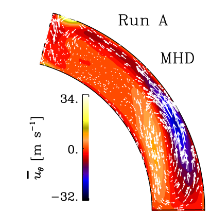
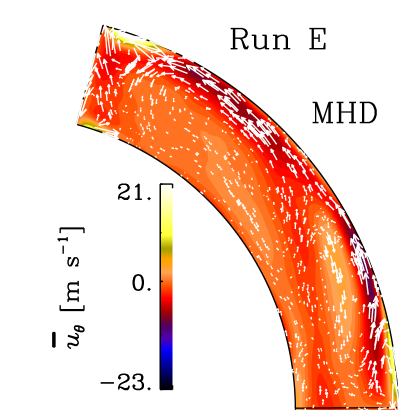
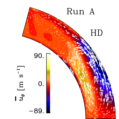
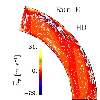
Figure 8: Meridional circulation from Runs A and E. The arrows show the direction of flow ${\overline{\bm{u}}}_{\rm m}\equiv(\bar{u}_{r},\bar{u}_{\theta})$ and the background color shows $u_{\theta}$. Upper (lower) panels are from magnetohydrodynamic (hydrodynamic) simulations.

Table 2: Summary of the diagnostic quantities of Runs A–E.

$$\begin{array}[]{p{0.05\linewidth}ccccccccccrccccccclc}\hline\cr\vskip 3.0pt plus 1.0pt minus 1.0pt\cr Run&P_{1}{\rm[yr]}(N)&P_{2}{\rm[yr]}(N)&P_{1}{\rm[yr]}(S)&P_{2}{\rm[yr]}(S)&B_{\rm eq}{\rm[G]}&\overline{B}_{\rm rms}{\rm[G]}&\frac{E_{\rm mag}}{E_{\rm kin}}&\frac{E_{\rm pol}}{E_{\rm kin}}&\frac{E_{\rm tor}}{E_{\rm kin}}&\frac{E_{\rm mer}^{\rm HD}}{E_{\rm mer}^{\rm MHD}}&\frac{E_{\rm rot}^{\rm HD}}{E_{\rm rot}^{\rm MHD}}&{\rm P_{asym}}\\ \hline\cr A&{\bf 2.96\pm 0.22}&4.04\pm 0.70&{\bf 2.85\pm 0.25}&4.05\pm 0.24&3931&11412&0.119&0.066&0.052&12.1&\leavevmode\nobreak\ 92.4&{\rm no}\\ B&5.45\pm 0.20&{\bf 7.88\pm 0.57}&{\bf 6.5\pm 1.5}&8.7\pm 1.4&2956&11339&0.068&0.038&0.030&16.1&114.8&{\rm no}\\ BC&10.6\pm 0.33&-&10.8\pm 0.66&-&2724&11150&0.060&0.033&0.026&-&-&{\rm no}\\ C&7.0\pm 1.1&-&-&-&1789&10686&0.028&0.017&0.012&37.6&\leavevmode\nobreak\ 36.9&{\rm yes}\\ D&6.9\pm 1.1&-&9.4\pm 1.3&-&3152&9220&0.120&0.064&0.053&\leavevmode\nobreak\ 2.2&\leavevmode\nobreak\ \leavevmode\nobreak\ 1.2&{\rm yes}\\ E&{\bf 4.49\pm 0.38}&2.60\pm 0.67&2.58\pm 0.88&-&3472&8792&0.156&0.080&0.076&\leavevmode\nobreak\ 1.9&\leavevmode\nobreak\ \leavevmode\nobreak\ 2.2&{\rm yes}\\ \hline\cr\end{array}$$

For all the AS cases (Runs A, B, and BC) we find single cell meridional circulation with poleward flow near the surface and equatorward flow near the bottom of the convection zone. This is also the usual assumption in flux transport dynamo models (e.g., Dikpati & Charbonneau, 1999), although in such models only the equatorward motion at the bottom of the convection zone matters (Hazra et al., 2014). However, as we go to the SL differential rotation cases, i.e., from Run C to Runs D and E, the meridional circulation becomes weaker and shows multiple cells in radius and latitude, which has been detected in recent observations (Zhao et al., 2013; Schad et al., 2013; Kholikov et al., 2014). Guerrero et al. (2013) also find multi-cell meridional circulation for SL differential rotation and single or two-cell circulation for AS in their hydrodynamic simulations.

Table 1 shows that $E_{\rm mer}/E_{\rm kin}$ decreases rapidly from Runs A to E (with increasing ${\rm Co}$ the energy in the azimuthal component increases). The upper two panels of Fig. 8 show the meridional circulation for an AS (Run A) and a SL case (Run E). Note that, irrespective of the differential rotation profile, we obtain a poleward flow near the surface and its amplitude is in agreement with solar surface observations (see e.g., Hathaway & Rightmire, 2010; Zhao et al., 2013). The fact that it is poleward both for AS and SL rotation suggests that the meridional circulation is not just a consequence of differential rotation. This has been discussed in detail by Rüdiger (1989), who has shown that baroclinic forcing can also be an important driver for the origin of meridional circulation; see Miesch & Toomre (2009) (Sect. 3), who have demonstrated how in simulations the convective (and magnetic) angular momentum flux maintain meridional circulation in the solar convection zone through the gyroscopic pumping. We note that in our simulations we do not have the near-surface shear layer, which helps to produce a poleward flow in the upper layers through inward angular momentum transport possibly by the downflow plumes (Kitchatinov & Rüdiger, 2005; Miesch & Hindman, 2011; Hotta et al., 2014).

It is important to compare these results with the hydrodynamical counterparts of the same models shown in the two lower panels. We see that the hydrodynamic flow is much stronger, although the overall pattern is not very different. In Table 2, we compare the energy ratios $E_{\rm mer}^{\rm HD}/E_{\rm mer}^{\rm MHD}$ and $E_{\rm rot}^{\rm HD}/E_{\rm rot}^{\rm MHD}$ of meridional circulation and rotation respectively with their hydrodynamic counterparts. The magnetic field clearly suppresses the circulation in the AS cases, Runs A–BC, but also in Run C, whereas in the other SL cases the effect is small. Moreover, the flow shows significant temporal variation, which will be explored later in § 3.8.

3.6 Magnetic variability and butterfly diagrams

The large-scale spatio-temporal organization of the magnetic field can be seen from a time–latitude or butterfly diagram of $\overline{B}_{\phi}$, for example. The degree of radial coherence can be judged by looking at different depths. We show such butterfly diagrams for Runs A–E both at $r=0.74\leavevmode\nobreak\ R_{\odot}$ (Fig. 9) and at $r=0.96\leavevmode\nobreak\ R_{\odot}$ (Fig. 10), where $\overline{B}_{\phi}$ is given in Gauss. Here we only show the first 70 years of each simulation, although in some cases we ran for longer times (see below). We see that Runs A, B, and BC, which produce AS differential rotation, show prominent activity cycles, but no clear polarity reversals. Therefore, these activity cycles are different from the Hale polarity cycle of the Sun. However, we want to stress here that polarity reversals are verified only for the Sun, whereas for stellar cycles, most commonly detected either from photometry or from Ca H & K lines with spectroscopy, such information is not retrievable, and therefore the reported variability might equally well be related to variations in the magnetic field strength as to polarity reversals.

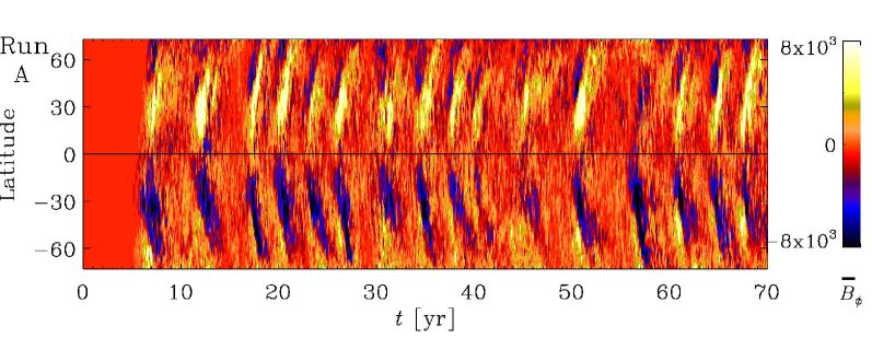
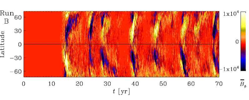
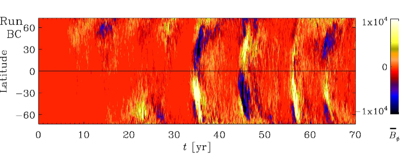
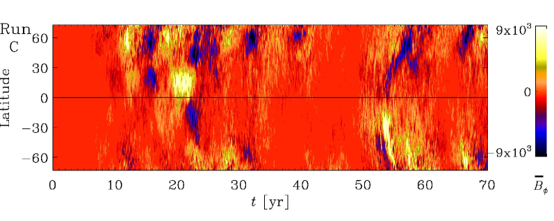
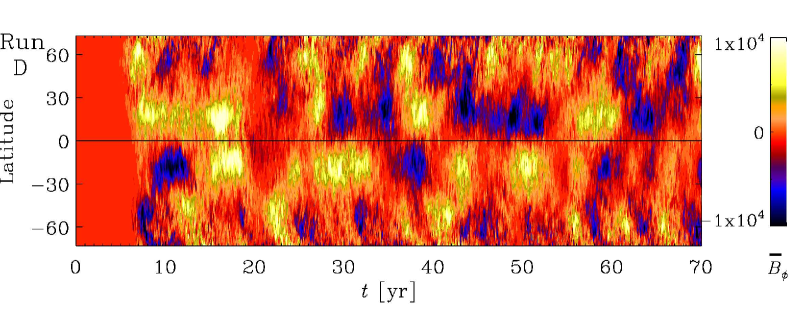
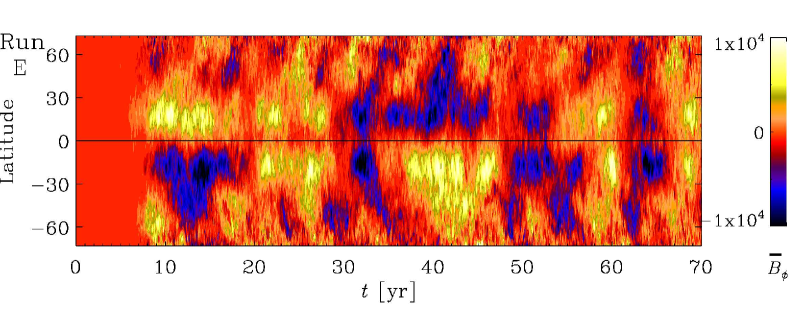
Figure 9: Butterfly diagrams: contours of the toroidal field $\overline{B}_{\phi}$ (in Gauss) at $r=0.74\leavevmode\nobreak\ R_{\odot}$ from Runs A, B, BC, C, D, and E (top to bottom).

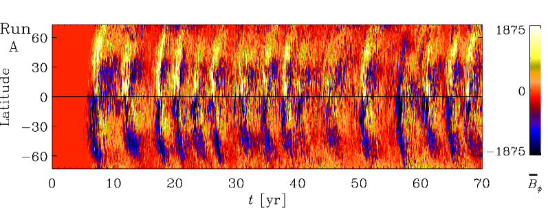
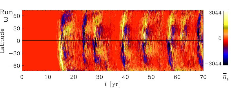
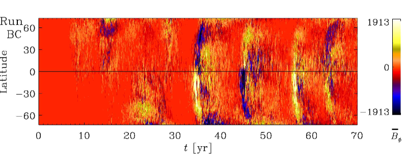
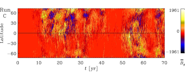
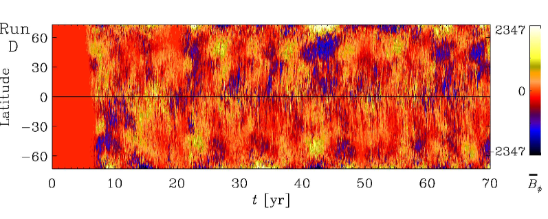
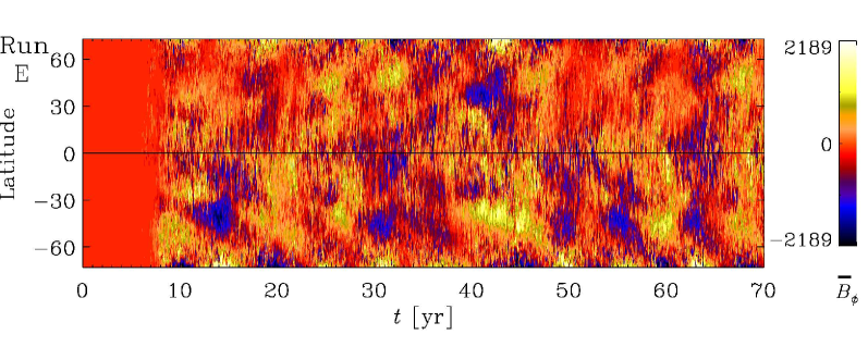
Figure 10: Same as Fig. 9 but here $\overline{B}_{\phi}$ is shown at $r=0.96\leavevmode\nobreak\ R_{\odot}$.

For Runs A and B, the activity cycles are associated with a weak poleward propagation at high latitudes. Another aspect we notice is that, as we go from Run A to Run BC, the activity cycles appear at a later time. This is surprising given that the rotational influence on the turbulence actually increases. For Run C, with SL rotation, the variations are rather irregular and show periods of very weak mean fields. The variations in Runs D and E are irregular and a different dynamo mode appears to be excited in these simulations, which is also characterized by a weaker influence on the differential rotation than in the AS cases. By comparing Figs. 9 and 10, we also see that $\overline{B}_{\phi}$ is stronger near the bottom of the convection zone, which could be caused by downward pumping of the mean magnetic field (Nordlund et al., 1992; Brandenburg et al., 1996; Tobias et al., 2001).

Comparing with earlier work, we note that in several recent global dynamo simulations (Ghizaru et al., 2010; Racine et al., 2011; Brown et al., 2011; Käpylä et al., 2012, 2013; Cole et al., 2014), regular cycles develop, resulting in butterfly diagrams with polarity reversals and sometimes even equatorward migration of toroidal field at low latitudes. However all these simulations are for larger Coriolis numbers (for example, ${\rm Co}\geq 5$ in Cole et al., 2014), in which regime more coherent fields have been found to be favored (Brown et al., 2010, 2011).

3.7 Diagnostic stellar activity diagrams

The nature of stellar cycles can be characterized by the ratio of cycle frequency $\omega_{\rm cyc}=2\pi/P$ to the rotation rate $\Omega_{0}$, where $P$ is an estimate of the cycle period. There is a tendency for stars of different characteristics to group at different positions in a “diagnostic” diagram of $\omega_{\rm cyc}/\Omega_{0}$ versus ${\rm Co}$ (Brandenburg et al., 1998; Saar & Brandenburg, 1999). The more rapidly rotating stars of Käpylä et al. (2013) were found to be located in three groups with increasing slope in two of them and decreasing slope in one.

In the present work, the values of ${\rm Co}$ are much smaller, so it is important to repeat such an analysis for the more slowly rotating stars of the present paper. However, even by visual inspection of the butterfly diagrams, it is evident that these variations are not strictly harmonic, and therefore Fourier transform is not useful for the analysis. Instead, we use the phase dispersion method (Pelt, 1983; Lindborg et al., 2013). It is based on the statistics

$$D^{2}(P)=\frac{1}{2\sigma^{2}}\frac{{\sum\limits_{i=1}^{N-1}{\sum\limits_{j=i+1}^{N}{g(t_{i}}},t_{j},P,\Delta t)[f(t_{i})-f(t_{j})]^{2}}}{{\sum\limits_{i=1}^{N-1}{\sum\limits_{j=i+1}^{N}{g(t_{i}}},t_{j},P,\Delta t)}},$$ (14)

where $f(t_{i}),i=1,\dots,N$ is the input time series, $\sigma^{2}$ is its variance, $g(t_{i},t_{j},P,\Delta t)$ is the selection function, which in the general case is significantly different from zero only when

$$t_{j}-t_{i} \approx kP,k=\pm 1,\pm 2,\ldots{\rm\ \ \ and}$$ (15)

$$\left|{t_{j}-t_{i}}\right| \leq \Delta t.$$ (16)

In the latter condition, $\Delta t$ is the so-called correlation length. In our case the time series is evenly sampled, in which case a modification to the general top-hat selection function is needed to prevent artefacts: in this study we choose $g$ as the product of two Gaussians: one with a half-width-at-half-maximum (HWHM) of $\Delta t$ and the other with an HWHM of a preselected phase separation limit, for which we adopt 0.1. For the particular case when $\Delta t$ is longer than the full data span, the $D^{2}(P)$ statistics is essentially a slight reformulation of the well known Stellingwerf statistics (Stellingwerf, 1978). As the correlation length is made shorter, we match nearby cycles in a progressively narrower region, and consequently estimate a certain mean period, which needs not to be coherent for the full time span. After having continued Runs C, D and E for a longer time, we apply this statistics to the time series of $\overline{B}_{\phi}^{2}$ at $r=0.96\leavevmode\nobreak\ R_{\odot}$, averaged over $10^{\circ}$ to $50^{\circ}$ latitude, separately for north and south. This is shown in the left column of Fig. 11, where we now depict the full length of the simulation, excluding however the initial exponential growth phase of the dynamo.

To determine the possible average period of the cycle in the time series we proceed as follows: first we calculate the $D^{2}$ statistics for preselected period and correlation length ranges. Then looking at the plot we detect the correlation lengths for which there exist only distinct flat minima around certain periods (this must be the case for the leftmost correlation length if the lower bound has been chosen correctly). After eliminating doubles or halves of the actual periods we obtain a set of candidate periods. The period with the strongest minimum is selected as the best candidate, others being possible modulating periods.

In Fig. 11, the results for the phase dispersion analysis are depicted; the periods with error estimates for all the runs can be found from Table 2. The error estimates were calculated by building bootstrap resamples for the differences between pairs of data points with approximately the same time separation. For Run A, a stable period of slightly less than three years is prominent especially for the southern hemisphere, which is manifested by the fact that the minimum does not split even if the correlation length is increased. For the northern hemisphere, a period with roughly the same value is obtained, but it is less coherent and splits at correlation lengths of roughly 25 years. A secondary period of roughly 4 years is also present in both hemispheres. The hemispheres appear less synchronized for Run B: again, two significant periods are detected for both hemispheres, the most prominent ones being 8 and 7 years, respectively (albeit with large error estimates). Again, the dominant periods persist even when the correlation length is increased. For Run BC, a stable period of about 11 years is found in both hemispheres. In the southern hemisphere, it is more persistent as the correlation length is increased. For Run C, only the northern hemisphere shows a prominent period around 7 years, while the splitting of the minima starts already for the correlation length of 10 years in the south. Run D shows prominent periods around 7 and 9 years for the northern and southern hemispheres, respectively. Although splitting occurs especially in the north, we regard these periods as significant. Finally in the case of Run E, multiperiodicity was detected for northern hemisphere with stronger period around 4.5 years and a weaker one around 2.5 years, while the latter period was detected also for the southern hemisphere.

The plot of $\omega_{\rm cyc}/\Omega_{0}$ versus ${\rm Co}$ is shown in Fig. 12(a), where we see that stars with AS and SL rotation are located in two different positions in such a diagram. We know that the Sun lies on the upper left branch in such a diagram for real stars (Brandenburg et al., 1998), but in Fig. 12(a) this branch corresponds to AS rotation, which obviously disagrees with the observations. However, it is plausible that there are stars with AS rotation that have simply not yet been observed. Our simulations therefore suggest a possible prediction in that such stars might occupy a possibly separate branch further to the left of the solar branch, which already corresponds to the domain of inactive stars. We thus expect there to be either a separate branch or a part of the branch with inactive stars like the Sun, having however AS rotation.

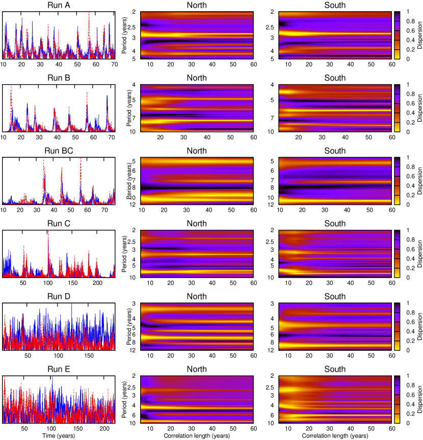
Figure 11: Phase dispersion analysis results; from top to bottom, Runs A–E, in the middle column for the northern hemisphere, on the right for the southern hemisphere. On the left column we show the original time series analyzed (blue/red for north/south). The time series are normalized by their means, so values are not shown.

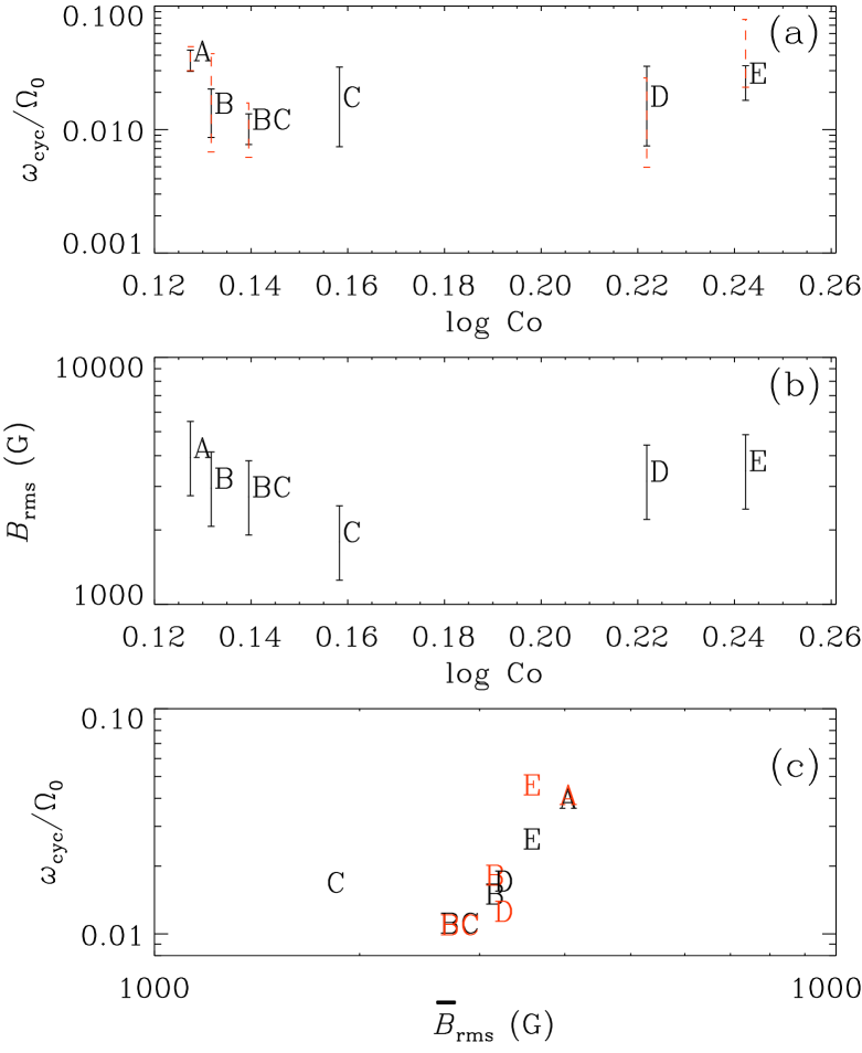
Figure 12: Diagnostic diagrams showing (a) $\omega_{\rm{cyc}}/\Omega_{0}$, (b) the strength of the large-scale magnetic field over the whole convection zone measured by $\overline{B}_{\rm rms}=\langle\langle B_{r}\rangle_{\phi}^{2}+\langle B_{\theta}\rangle_{\phi}^{2}+\langle B_{\phi}\rangle_{\phi}^{2}\rangle_{r\theta t}^{1/2}$ vs. log ${\rm Co}$, and (c) $\omega_{\rm{cyc}}/\Omega_{0}$ vs. $\overline{B}_{\rm rms}$. The red color shows the values computed for the southern hemisphere.

In Fig. 12(b) we show the mean magnetic field. Here the errors of $\overline{B}_{\rm rms}$ are computed as the largest departure of the mean from any one third of the full time series. We see that for the AS differential rotation runs (Runs A, B, and BC) the magnetic field decreases with rotation rate, whereas for the SL rotation cases (Runs C, D, and E) it increases.

In Fig. 12(c) we plot the cycle frequency ratio against the mean magnetic field. Following the interpretation of Brandenburg et al. (1998), the cycle frequency ratio is essentially a measure of the $\alpha$ effect in a mean-field dynamo, so the increasing trend in the cycle frequency ratio suggests that the $\alpha$ effect increases with magnetic field strength, which is referred to as antiquenching. This interpretation hinges on some ill-known assumptions, for example the turbulent transport in this model is assumed to depend only on the largest scale of the mean magnetic field and of course the rather unconventional assumption of antiquenching itself. Antiquenching of both $\alpha$ and turbulent diffusivity has actually been detected in simulations (Chatterjee et al., 2011), and may be possible more easily in a sphere than in a Cartesian layer, but we have at present no further indication that this interpretation is applicable to our model.

3.8 Magnetic modulation of the flow

We have seen that some of our runs show clear activity cycles. Therefore we expect to see a corresponding modulation of the flow. In Fig. 13, we show for Run A the temporal variation of the mean large-scale magnetic field ($\overline{B}$) normalized by $B_{\rm eq}$, the latitudinal component of the meridional circulation $u_{\theta}(r,\pm 32^{\circ})$ at $r\approx 0.95R_{\odot}$ and $r\approx 0.73R_{\odot}$, the mean rotation rate $\overline{\Omega}(0.95R_{\odot},\pm 32^{\circ})$, as well as the latitudinal and radial differential rotation $\Delta_{\Omega}^{(r)}$ and $\Delta_{\Omega}^{(\theta)}$, defined in Eq. (13). We see that the meridional circulation varies with the magnetic field, becoming weaker during maximum and stronger during minimum, the overall temporal variation being about $50\%$ in this case. (The linear correlation coefficient between $\overline{B}$ and $u_{\theta}(0.95R_{\odot},\pm 32^{\circ})\approx-0.36,-0.38$.) This kind of weak anti-correlation between the activity cycle and the meridional flow has been found in solar observations (Chou & Dai, 2001; Hathaway & Rightmire, 2010) and is believed to arise at least in part from the Lorentz force of the dynamo-generated magnetic fields (see e.g., Rempel, 2006; Karak & Choudhuri, 2012; Passos et al., 2012). The meridional circulation at the bottom is also weakly correlated with the activity cycle (correlation coefficients between $\overline{B}$ and $u_{\theta}(0.73R_{\odot},\pm 32^{\circ})\approx-0.22,-0.47$). We see that $\overline{\Omega}(0.95R_{\odot},\pm 32^{\circ})$ (Fig. 13(c)) also shows a weak anti-correlation with the magnetic variations (having correlation coefficient $\approx-0.25$). The strong magnetic fields during maxima change $\overline{\Omega}$ by a few per cent ($\approx 6\%$). However $\overline{\Omega}(0.95R_{\odot},0^{\circ})$ (Fig. 13(d)) shows positive correlation (correlation coefficient $\approx 0.36$) and the overall variation is larger ($\approx 12\%$). Due to this variation of $\overline{\Omega}$ at the equator, the values of $\Delta_{\Omega}^{(r)}$ and $\Delta_{\Omega}^{(\theta)}$ (Fig. 13e-f) show a positive correlation with the magnetic field (correlation coefficients 0.36, 0.21) with the overall variation being $\sim 75\%$ and $166\%$, respectively.

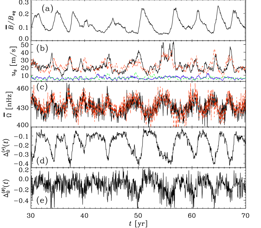
Figure 13: From Run A: (a) The large-scale magnetic field over the whole convection zone $\overline{B}=\langle\langle B_{r}\rangle_{\phi}^{2}+\langle B_{\theta}\rangle_{\phi}^{2}+\langle B_{\phi}\rangle_{\phi}^{2}\rangle_{r\theta}^{1/2}$ normalized by $B_{\rm eq}$. (b) The latitudinal component of meridional circulation $u_{\theta}(r,\pm 32^{\circ})$ (smoothed over 5 months) at $r\approx 0.95R_{\odot}$ (black and red) and $r\approx 0.73R_{\odot}$ (blue and green), (c) azimuthally averaged angular velocity $\overline{\Omega}(0.95R_{\odot},\pm 32^{\circ})$, (d) $\overline{\Omega}(r,0^{\circ})$ at $r=0.73R_{\odot}$ (red dashed) and $r=0.95R_{\odot}$ (black). The dashed (solid) line corresponds to the southern (northern) hemisphere. (e) Radial shear $\Delta_{\Omega}^{(r)}$, and (f) latitudinal shear $\Delta_{\Omega}^{(\theta)}$, defined in Eq. (13), as functions of time.

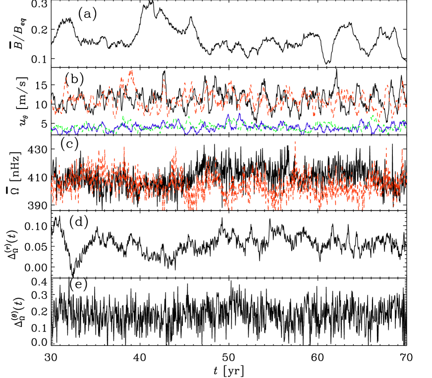
Figure 14: Same as Fig. 13, but from Run E which produces SL differential rotation.

We have seen that Runs B, BC, and C produce clear activity cycles similar to Run A and in all these runs we do see a corresponding variation in the flow. However, for Runs C, D, and E, which produce SL differential rotation, the magnetic variations are not so regular. In Fig. 14, we show the temporal variations for the SL differential rotation case Run E. We see that the large-scale magnetic field does not have a regular cycle. The meridional circulation does not appear to show a close correlation with the magnetic field (with correlation coefficients being about $-0.1$ and $-0.3$ for surface and bottom meridional circulation, respectively). However the significant variations (up to $45\%$) exist. Such irregular variation in meridional circulation is found to be crucial in modeling many aspects of the solar cycle in flux transport dynamo model (Karak & Choudhuri, 2011, 2013). The situation is similar in the case of differential rotation and rotational shear: the early part of the time series ($t=30\ldots 50$ yr) show an anti-correlation with the magnetic field strength, but at later times this correlation is not so obvious (the overall linear correlation coefficients are $-0.32$, $-0.22$, $-0.43$, $0.28$, $-0.55$ and $0.19$ for $\overline{\Omega}(0.95R_{\odot},\pm 32^{\circ})$, $\overline{\Omega}(0.95R_{\odot},0^{\circ})$, $\overline{\Omega}(0.73R_{\odot},0^{\circ})$, $\Delta_{\Omega}^{(r)}$, and $\Delta_{\Omega}^{(\theta)}$, respectively). The variation in differential rotation is about $4\%$, whereas for the radial and latitudinal shear it is about $50\%$ and $60\%$, respectively.

Significant variations observed in the large-scale flows in all the simulations motivate us to measure the Lorentz force. The Lorentz force can change the flow by acting in two ways, through large-scale and small-scale magnetic fields. Firstly, it can act directly on the large-scale flow which is known as ‘macro-feedback’ (caused by the mean Lorentz force) and has been applied in several mean-field models (e.g., Schüssler, 1979; Brandenburg et al., 1992). Secondly, it can affect the large-scale flow by affecting the convective motions and the best example of this is the magnetic quenching of the $\Lambda$-effect, which is known as ‘micro-feedback’ (for an application, see Küker et al., 1999).

To get an idea of these effects we measure the $\phi$ component of the Lorentz force (which appears in the zonal momentum equation) from the large-scale magnetic field $(\overline{\bm{J}}\times\overline{\bm{B}})_{\phi}$, and the small-scale contribution $(\overline{{\bm{j}}\times{\bm{b}}})_{\phi}$ which are shown in Fig. 15 both during magnetic maximum (left two panels) and minimum (right two panels) from Run A. We see that the small-scale Lorentz force, which enters into the total stress and thus the $\Lambda$ effect, is typically stronger than the Lorentz force of the large-scale field and both have significant temporal variations, becoming weaker during magnetic minimum. Clearly both contributions are important, which was already emphasized by Beaudoin et al. (2013), who discussed in detail the differences in the integrated stresses for hydrodynamic and magnetic models in the case of SL rotation. Our results also show that both small-scale and large-scale contributions to the Lorentz force are responsible for producing temporal variations in the large-scale flows. Beaudoin et al. (2013) also emphasized the importance of magnetic fields in providing coupling to the radiative interior which is absent in their hydrodynamic models, but also in our magnetic models which lack the presence of a lower overshoot layer. Finally, we note that, while the Lorentz force from the mean field shows, during magnetic maximum, a systematic variation with distance from the axis, there are variations on similarly small scales both from the mean and fluctuating fields. This property is related to poor scale separation and may also apply to real stars.

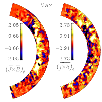
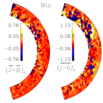
Figure 15: From Run A: Contributions of the $\phi$ component of the large-scale Lorentz force $\overline{\bm{J}}\times\overline{\bm{B}}$ and small-scale Lorentz force $\overline{{\bm{j}}\times{\bm{b}}}$ during a magnetic maximum (left two panels) and minimum (right two panels). Values are given in units of $10^{-9}$ N m^-3.

4 Turbulent angular momentum transport

Numerical simulations have been used on various occasions to study angular momentum transport in both hydrodynamic and magnetic cases, but they usually focus on the regime of SL rotation (Brun & Toomre, 2002; Brun et al., 2004; Beaudoin et al., 2013). Furthermore, the contributions to the stress are often integrated over latitude or radius. In such representations, the stresses from opposite signs tend to cancel.

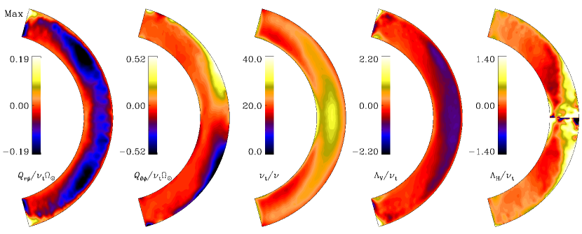
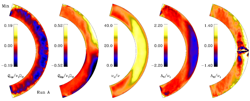
Figure 16: Normalized profiles of $Q_{r\phi}$, $Q_{\theta\phi}$, $\nu_{\rm t}$, $\Lambda_{\rm V}$, and $\Lambda_{\rm H}$ for Run A. The top and bottom panels show data averaged over four maxima and minima, respectively.

To make contact with mean-field theory invoking the $\Lambda$ effect (Rüdiger, 1980, 1989), it is useful to look at the profiles without integration over latitude or radius and to separate between diffusive and nondiffusive contributions. Simulations have confirmed many aspects of $\Lambda$ effect in mean field theory (Pulkkinen et al., 1993; Rieutord et al., 1994). The aim here is to interpret the differences between hydrodynamic and magnetic cases in the AS and SL regimes in terms of corresponding changes in the underlying $\Lambda$ effect. For this purpose we first compute the contributions of the Reynolds stress $Q_{ij}=\overline{u_{i}^{\prime}u_{j}^{\prime}}$, and the Maxwell stress $M_{ij}=(\rho\mu_{0})^{-1}\overline{B_{i}^{\prime}B_{j}^{\prime}}$ to the angular momentum balance in the convection zone. Here, primes denote fluctuating quantities which are calculated by subtracting the longitudinal mean from the original quantity, e.g., $u_{i}^{\prime}=u_{i}-\overline{u}_{i}$. The radial and latitudinal angular momentum transports are determined by the off-diagonal components of $Q_{ij}$ and $M_{ij}$, namely $Q_{r\phi}$, $Q_{\theta\phi}$, $M_{r\phi}$ and $M_{\theta\phi}$, respectively. In the mean-field theory of hydrodynamics, the Reynolds stress contributions to angular momentum transport are approximated in terms of the turbulent viscosity $\nu_{\rm t}$ and the $\Lambda$-effect (Rüdiger, 1980, 1989):

$$Q_{r\phi} = \overline{u_{r}^{\prime}u_{\phi}^{\prime}}\equiv\Lambda_{\rm V}\sin\theta\overline{\Omega}-\nu_{\rm t}r\sin\theta\frac{\partial\overline{\Omega}}{\partial r},$$ (17)

$$Q_{\theta\phi} = \overline{u_{\theta}^{\prime}u_{\phi}^{\prime}}\equiv\Lambda_{\rm H}\cos\theta\overline{\Omega}-\nu_{\rm t}\sin\theta\frac{\partial\overline{\Omega}}{\partial\theta}.$$ (18)

The coefficients $\Lambda_{\rm V}$ and $\Lambda_{\rm H}$ are the vertical and horizontal $\Lambda$-effects, which are non-diffusive contributions to the Reynolds stress that arise from the interaction of anisotropic turbulence and rotation (Kitchatinov & Rüdiger, 1995). As in earlier work (Käpylä et al., 2014), we adopt the mixing length formula to estimate $\nu_{\rm t}$

$$\nu_{\rm t}={\textstyle{1\over 3}}u_{\rm rms}\alpha_{\rm MLT}H_{p},$$ (19)

where $\alpha_{\rm MLT}=1.7$ and $H_{p}(r)=-(\partial\ln p/\partial r)^{-1}$. By computing $u_{\rm rms}=u_{\rm rms}(r,\theta)$ using $\phi$ averages, we get the profile of $\nu_{\rm t}$ in the meridional plane.

The two leftmost panels of Fig. 16 show $Q_{r\phi}$ and $Q_{\theta\phi}$ normalized by $\nu_{\rm t}\Omega_{0}$, and the third panel shows $\nu_{\rm t}$ normalized by the microphysical viscosity $\nu$ from Run A. We see that $Q_{r\phi}$ is negative in most of the convection zone which implies inward transport of angular momentum. This is expected given the fact that the differential rotation in this case is AS. The negative $Q_{r\phi}$ is in agreement with Rieutord et al. (1994) and Käpylä et al. (2014). However for Run E, which produces SL differential rotation, $Q_{r\phi}$ is positive at low latitudes. On the other hand, the latitudinal stress $Q_{\theta\phi}$ is positive (negative) in the northern (southern) hemisphere, which implies equatorward angular momentum transport. This is true for both Runs A and E (Figs. 16 and 17). We note that the recent observation of $Q_{\theta\phi}$ (Hathaway et al., 2013) finds the same sign.

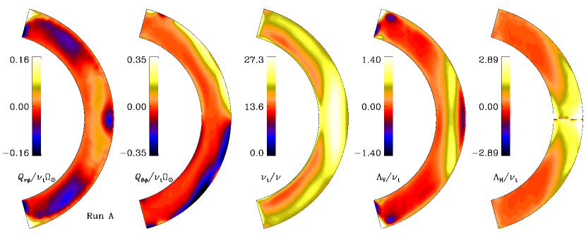
Figure 17: Similar to Fig. 16, but for Run E and time-averaged over the last few maxima and minima.

The magnetic field is expected to change the total (Reynolds and Maxwell) stress over the activity cycle. In fact, magnetic quenching of the Reynolds stress is known to have important consequences in mean-field models, particularly in connection with explaining the origin of the torsional oscillation of the Sun or grand minima (e.g., Kitchatinov et al., 1999; Küker et al., 1999). Therefore, to see the variations over the activity cycle, we show $Q_{r\phi}$ and $Q_{\theta\phi}$ both during maximum and minimum phases. Note that these are not computed from one snapshot, but from averages over four maxima or minima phases. By comparing top and bottom panels of Fig. 16 we find that $Q_{r\phi}$ is slightly stronger during magnetic maximum, although $Q_{\theta\phi}$ is weaker. Even if we ignore the fact that our model is very far from that of Beaudoin et al. (2013), a quantitative comparison of our results is not straightforward. Moreover, Beaudoin et al. (2013) show the temporal variations of fluxes integrated across spherical shells; see their definition of $I_{r}$ in Eq. (22) and Figure 7. During magnetic maximum, our $Q_{r\phi}$ becomes stronger, whereas $I_{r}$ in Beaudoin et al. (2013) becomes weaker and its overall variation is higher than ours. The temporal variations of Reynolds stresses show spatial coherence over all depths as seen in Beaudoin et al. (2013).

Next, we see in the middle panels of Fig. 16 that $\nu_{\rm t}$ is significantly weaker during maximum due to magnetic quenching. The normalized value is around 40, which is similar to the value of ${\rm Re}$. We note that $\nu_{\rm t}$ decreases towards high latitudes, but increases towards deeper regions of the convection zone.

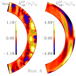
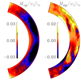
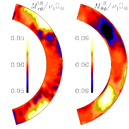
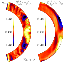
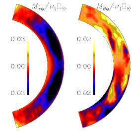
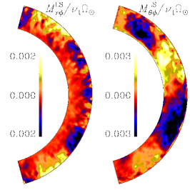
Figure 18: From Run A: $R_{r\phi}^{\rm LS}=\overline{u}_{r}(\overline{u}_{\phi}+\Omega_{0}r\sin\theta)$, $R_{\theta\phi}^{\rm LS}=\overline{u}_{\theta}(\overline{u}_{\phi}+\Omega_{0}r\sin\theta)$ (left two panels), $M_{r\phi}=\overline{B^{\prime}_{r}B^{\prime}_{\phi}}/\rho\mu_{0}$, $M_{\theta\phi}=\overline{B^{\prime}_{\theta}B^{\prime}_{\phi}}/\rho\mu_{0}$ (middle two), $M_{r\phi}^{\rm LS}=\overline{B}_{r}\overline{B}_{\phi}/\rho\mu_{0}$ and $M_{\theta\phi}^{\rm LS}=\overline{B}_{\theta}\overline{B}_{\phi}/\rho\mu_{0}$ (right two), normalized by $\nu_{\rm t}\Omega_{\odot}$. Upper and lower panels are during magnetic maximum and minimum, respectively.

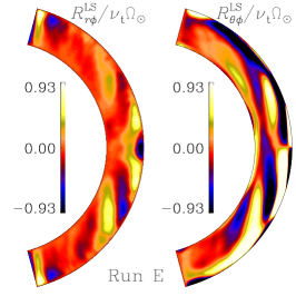
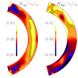
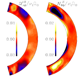
Figure 19: Same as Fig. 18 but from Run E and averaged over last few maxima and minima.

After solving Eqs. (17) and (18) for $\Lambda_{\rm V}$ and $\Lambda_{\rm H}$ by using the computed values of $Q_{r\phi}$, $Q_{\theta\phi}$, and $\nu_{\rm t}$, we find $\Lambda_{\rm V}$ and $\Lambda_{\rm H}$ again during magnetic maximum and minimum. These are shown in the last two panels of Fig. 16. We see that $\Lambda_{\rm V}$ is negative in most of the convection zone, which is in agreement with the findings from the first-order smoothing approximation (Kitchatinov & Rüdiger, 1995, 2005), and with earlier numerical studies (e.g., Pulkkinen et al., 1993; Käpylä et al., 2004; Rüdiger et al., 2005; Käpylä & Brandenburg, 2008; Käpylä et al., 2014). However, for Run E with SL rotation, $\Lambda_{\rm V}$ is positive at low latitudes and does not change much from maximum to minimum, which is why we show in Fig. 17 averages over all time. Another important property is that $\Lambda_{\rm V}$ is of the same order as $\nu_{\rm t}$, which is consistent with earlier findings (Käpylä et al., 2010a). We find that for both Runs A and E, $\Lambda_{\rm H}$ is positive which is again in agreement with the analytical results. By comparing the present results with the hydrodynamic counterparts of Käpylä et al. (2014), we find that the $\Lambda$-effect, is weaker. This could be a reason for getting strongly suppressed differential rotation, compared to the hydrodynamic simulations, particularly in AS cases (Runs A–BC). Furthermore we see a significant cycle-related variation in the $\Lambda$-effect. In AS cases, both $\Lambda_{\rm V}$ and $\Lambda_{\rm H}$ are much smaller during maximum (see last two columns in Fig. 16). This could be one of the reasons for significant temporal variations in the large-scale flow.

Next we compute the radial and latitudinal components to the angular momentum transport by the meridional circulation: $R_{r\phi}^{\rm LS}=\overline{u}_{r}(\overline{u}_{\phi}+\Omega_{0}r\sin\theta)$, and $R_{\theta\phi}^{\rm LS}=\overline{u}_{\theta}(\overline{u}_{\phi}+\Omega_{0}r\sin\theta)$. We show these in Fig. 18 for Run A both during magnetic maximum and minimum. Again, they are normalized by $\nu_{\rm t}\Omega_{\odot}$ using the $\nu_{\rm t}$ computed earlier. We see that these stresses, particularly the latitudinal component, are the most dominating ones for transporting angular momentum. This is because in this run we have strong meridional circulation, mostly poleward near surface and equatorward near the bottom. We also observe temporal modulations of transport due to meridional circulation, which become stronger during magnetic minimum. Therefore this temporal variation could lead to a variation in the differential rotation. In fact, Beaudoin et al. (2013) found significant temporal variation in the angular momentum flux from meridional circulation and suggested that it could be the primary source of the torsional oscillations. The temporal variations of $R_{r\phi}^{\rm LS}$ are not well-correlated spatially, which is also seen in Beaudoin et al. (2013) (see Fig. 7B). For Run E, which is shown in Fig. 19, we find smaller values of the stresses from the mean flows than in Run A, which is expected because of a much weaker meridional circulation in this case.

In the middle four panels of Fig. 18 we show the radial and latitudinal components of the Maxwell stress: $M_{r\phi}=\overline{B^{\prime}_{r}B^{\prime}_{\phi}}/\rho\mu_{0}$ and $M_{\theta\phi}=\overline{B^{\prime}_{\theta}B^{\prime}_{\phi}}/\rho\mu_{0}$, respectively from Run A, both during magnetic maximum and minimum. We see that these are an order of magnitude smaller than $Q_{r\phi}$ and $Q_{\theta\phi}$ and they have the same signs as $Q_{r\phi}$ and $Q_{\theta\phi}$, respectively. During magnetic maximum, both $M_{r\phi}$ and $M_{\theta\phi}$ (top middle panels of Fig. 18) are significantly larger than during magnetic minimum (lower middle panels). Therefore the Maxwell stresses may be another source of the temporal variation in the differential rotation. We recall that Beaudoin et al. (2013) also find large variations of the Maxwell stress in their simulation with highly correlated spatial variations. In Run E, shown in middle panels of Fig. 19, we again find similar values of $M_{r\phi}$ and $M_{\theta\phi}$ and acting in the opposite to $Q_{r\phi}$ and $Q_{\theta\phi}$, respectively.

The Maxwell stress discussed above contributes to the redistribution of angular momentum by fluctuating (non-axisymmetric) magnetic fields. The mean axisymmetric field also contributes to the angular momentum balance (see e.g., Brun et al., 2004; Beaudoin et al., 2013). This mean contribution is the result of correlations of the mean toroidal field with the radial and latitudinal components of the mean magnetic fields which are $M_{r\phi}^{\rm LS}=\overline{B}_{r}\overline{B}_{\phi}/\rho\mu_{0}$ and $M_{\theta\phi}^{\rm LS}=\overline{B}_{\theta}\overline{B}_{\phi}/\rho\mu_{0}$. The two rightmost columns of panels of Fig. 18 show these two terms from Run A, both during magnetic maximum and minimum. For Run E, they are shown in the two rightmost panels of Fig. 19. Again we see that both components of the stress from the mean field are much smaller than the Reynolds stresses $Q_{r\phi}$ and $Q_{\theta\phi}$ and comparable to the fluctuating contributions, $M_{r\phi}$ and $M_{\theta\phi}$. Importantly, they become much weaker during magnetic minimum. The variation in the large-scale magnetic tension is much larger than the variations in the other stresses and also much larger than what Beaudoin et al. (2013) found. They concluded that the variation in the large-scale magnetic tension is not responsible for the torsional oscillations. By comparing the top and bottom rows of the four rightmost panels of Fig. 18 we see that the temporal coherence of the spatial structures is not preserved during the activity cycle, which was also observed by Beaudoin et al. (2013). However, we must bear in mind that here we are comparing our Run A, which produces AS differential rotation, with a SL case in Beaudoin et al. (2013). In our SL cases, there are no prominent cycles and the temporal variations in the stresses are less pronounced than in Run A.

5 Conclusion

Motivated by the recently discovered bistability of stellar differential rotation in hydrodynamic spherical convection simulations (Gastine et al., 2014; Käpylä et al., 2014), we have performed several sets of magnetohydrodynamic simulations. Except for the allowance of dynamo-generated magnetic fields, our models are essentially the same as those of Käpylä et al. (2014). By taking different radiative conductivities, the convective velocities and hence the rotational influence are varied in the simulations. Runs A, B, and BC (${\rm Co}=1.34$, 1.35, and 1.38) produce AS differential rotation, whereas Runs C, D, and E (${\rm Co}=1.44$, 1.67, and 1.75) produce SL differential rotation. When we take an AS (SL) rotation profile as initial condition and perform a set of simulations by increasing (decreasing) the radiative conductivity slowly, we find similar states of differential rotation as in simulations which were started from scratch, i.e., with an initially rigid rotation profile. Therefore the bistable states of differential rotation seem to disappear in the MHD simulations, and we only find mono-stable solutions.

Besides the disappearance of the bistable differential rotation in MHD simulations, we find several other new results. (i) The abrupt transition from AS to SL rotation in hydrodynamic simulations now seems to become more gradual and this transition happens at slightly larger values of ${\rm Ro}_{\rm c}$ ($\approx 0.66$) and thus smaller values of ${\rm Co}$ ($\approx 1.4$). This means that the magnetic field helps to produce SL differential rotation, which is also in agreement with the recent study of Fan & Fang (2014). (ii) The polar vortices or jet-like structures that were observed in previous hydrodynamic simulations (e.g., Heimpel & Aurnou, 2007; Käpylä et al., 2014) are now absent. (iii) Both differential rotation and meridional circulation are now strongly suppressed in comparison to the hydrodynamic values and lie within the observed range. The suppression of these large-scale flows in the magnetic runs, particularly in AS differential rotation cases, could be a consequence of a reduction of the $\Lambda$ effect and the presence of the Lorentz force of the magnetic field acting on the flow (Malkus & Proctor, 1975). (iv) The large-scale flows show significant time variation as a consequence of the magnetic variations. All cases with AS differential rotation (Runs A–BC) show clear activity cycles and their large-scale flows have corresponding variations. Run A, which is more solar-like in terms of its highest convective flux and lowest ${\rm Co}$ value, shows $\approx 6\%$ variation in $\overline{\Omega}(r,\theta)$ about its mean. However the variation in meridional circulation is as large as $60\%$ and in large-scale shear, $\Delta_{\Omega}^{(r)}$ and $\Delta_{\Omega}^{(\theta)}$, the variations are about $75\%$ and $160\%$, respectively. All runs which produce SL differential rotation (Runs C–E) also show some magnetic variations, although they are not as regular and prominent as for AS differential rotation. In these runs we also see a detectable temporal variation in the large-scale flows which is primarily caused by the variations of the large-scale (axisymmetric) magnetic tension, the Maxwell stresses, and the stress from the mean flow. For Run E, which has the smallest convective flux and SL differential rotation, the variation in $\overline{\Omega}(r,\theta)$ is about $4\%$, whereas in both meridional circulation and large-scale shear the variation is about $50\%$.

Many authors simulate the large-scale flows in stellar convection zones using hydrodynamical models assuming that the magnetic field does not have a significant effect (Brun & Toomre, 2002; Ballot et al., 2007; Gastine et al., 2013, 2014; Guerrero et al., 2013; Käpylä et al., 2014, to mention just a few). It is difficult to quantify the effects of dynamo-generated magnetic fields on flows in the Sun from simulations as all the existing models are still far from the real Sun. However, from observations (Chou & Dai, 2001; Hathaway & Rightmire, 2010; Antia et al., 2008) we do see significant variations in both meridional circulation and rotational shear as well as a small variation in differential rotation in the form of torsional oscillations, which are believed to be (at least partially) coming from cyclic variations of the magnetic fields. The present study now suggests that magnetic fields cannot be neglected in simulating the large-scale flows in solar convection zone.